The Gerasimov-Drell-Hearn Sum Rule and the Spin Structure of the Nucleon

Abstract

The Gerasimov-Drell-Hearn sum rule is one of several dispersive sum rules that connect the Compton scattering amplitudes to the inclusive photoproduction cross sections of the target under investigation. Being based on such universal principles as causality, unitarity, and gauge invariance, these sum rules provide a unique testing ground to study the internal degrees of freedom that hold the system together. The present article reviews these sum rules for the spin-dependent cross sections of the nucleon by presenting an overview of recent experiments and theoretical approaches. The generalization from real to virtual photons provides a microscope of variable resolution: At small virtuality of the photon, the data sample information about the long range phenomena, which are described by effective degrees of freedom (Goldstone bosons and collective resonances), whereas the primary degrees of freedom (quarks and gluons) become visible at the larger virtualities. Through a rich body of new data and several theoretical developments, a unified picture of virtual Compton scattering emerges, which ranges from coherent to incoherent processes, and from the generalized spin polarizabilities on the low-energy side to higher twist effects in deep inelastic lepton scattering.

1. INTRODUCTION

The Gerasimov-Drell-Hearn (GDH) sum rule relates the anomalous magnetic moment (a.m.m.) of a particle to an energy-weighted integral over its photoabsorption cross sections Ger65 . This relation bears out that a finite value of the a.m.m. requires the existence of an excitation spectrum, and that both phenomena are simply different aspects of a particle with intrinsic degrees of freedom. A further property of composite objects is their spatial extension in terms of size and shape, which reveals itself through form factors measured by elastic lepton scattering. The less known Burkhardt-Cottingham (BC) sum rule connects a particular combination of these form factors to another energy-weighted integral over the total absorption cross sections for virtual photons BC70 . The discovery of the proton’s large a.m.m. Ste33 marked the beginning of hadronic physics. Today, 70 years later, we are still struggling to describe the structure of strongly interacting particles in a quantitative way.

Although quantum chromodynamics (QCD) is generally accepted as the underlying theory of the strong interactions, its low-energy aspects are difficult to deal with because of the large coupling constant in that region. However, the low-energy region is the natural habitat of protons and neutrons, and therefore of practically all visible matter in the universe. A plethora of models have been inspired by QCD, but none can be quantitatively derived from it. Only two descriptions are, in principle, exact realizations of QCD, namely chiral perturbation theory (ChPT) and lattice gauge theory. The former is an expansion in small external momenta and small (current) quark masses, and therefore it is limited to the threshold region and to the light $u$, $d$, and $s$ quarks. The effective degrees of freedom are the Goldstone bosons (quark-antiquark oscillations), notably the pions; all other possible structures are absorbed in contact interactions with “low-energy constants” (LECs) as proportionality factors. Lattice gauge theory, on the other hand, prescribes how to evaluate the QCD Lagrangian numerically on a space-time lattice in terms of quarks and gluons. For computational reasons the calculations have been mostly performed in the so-called quenched approximation, with only the minimal configuration of three quarks in configuration space. With algorithms such as “improved actions” for the light quarks and an increase in computing power by tera-flop machines, it is slowly becoming possible to include sea-quark degrees of freedom as well. Such effects have proved to be indispensable for an accurate description of hadronic observables Dav04 .

The persistent difficulties in quantitatively understanding nucleon structure explain why we are interested in a relation like the GDH sum rule. Being based on such general principles as causality, unitarity, and Lorentz and gauge invariance, this sum rule should be valid for every model or theory respecting these principles and having a “reasonable” high-energy behavior. Therefore, the agreement or disagreement between theoretical predictions and the sum rule provides invaluable information on the quality of the approximations involved and whether or not the relevant degrees of freedom have been included. Similarly, if we compare the sum rule value with accurate experimental data for the photoabsorption cross sections up to a certain maximum energy, we learn whether the physics responsible for the a.m.m. is also the physics of photoproduction to that energy, or whether phenomena at higher energies and possibly new degrees of freedom come into the game.

The a.m.m. $\kappa$ can be read off the relation between the total magnetic moment $\vec{\mu}$ and the spin $\vec{S}$ of a particle in its center-of-mass (c.m.) frame,

$$\vec{\mu}=\frac{e}{M}\,(Q+\kappa)\,\vec{S}\ ,$$ (1)

where $eQ$ is the charge and $M$ the mass of the particle. The elementary charge $e=|e|$ is defined by $e^{2}/4\pi=\alpha_{fs}\approx 1/137$. We use “natural” units, $c=\hbar=1$, and the nuclear magneton is given by the “normal” magnetic moment of the proton, $\mu_{N}=e/2M_{p}$. We also recall that the ratio between the magnetic moment $\vec{\mu}$ and the orbital angular momentum $\vec{L}$ of a uniformly charged rotating body is $eQ/2M$, while the ratio between the “normal” magnetic moment $\vec{\mu}$ and the spin $\vec{S}$ takes twice that value. This factor is described by the gyromagnetic ratio $g=2$ as predicted from Dirac’s equation for a spin $1/2$ particle. According to “Belinfante’s conjecture” Bel53 a particle of general spin $S$ should have $g=1/S$. However, Ferrara et al. Fer92 have quite convincingly shown that $g=2$ is required for particles of any spin $S$ in order to obtain a reasonable high-energy behavior.

The GDH sum rule relates the a.m.m. to the inclusive cross sections $\sigma_{P}$ and $\sigma_{A}$ for spherically polarized photons impinging on particles with spin parallel (P) or antiparallel (A) to the spin or helicity of the photon,

$$\frac{\pi e^{2}\kappa^{2}}{M^{2}}\,S=\int^{\infty}_{\nu_{0}}\frac{d\nu}{\nu}\,\left(\sigma_{P}(\nu)-\sigma_{A}(\nu)\right)\ ,$$ (2)

where the integral runs over the photon energy in the laboratory frame, $\nu$, from the lowest threshold $\nu_{o}$ to infinity. Because the left-hand side (LHS) of this equation is positive, we can draw the qualitative conclusion that the photon prefers to be absorbed with its spin parallel to the target spin. Of course, the sum rule is much more quantitative. The same agent that is responsible for the a.m.m. on the LHS of Eq. (2) must also lead to an appropriate energy dependence of the helicity difference of the cross sections, $\sigma_{P}-\sigma_{A}$, such that the sum rule is fulfilled. However, keep in mind one caveat: A basic assumption in deriving Eq. (2) is that $\sigma_{P}-\sigma_{A}$ vanishes sufficiently fast such that the integral converges.

Having followed through to this point, the reader may well ask whether we can ever be sure that the GDH sum rule is fulfilled. In a sense we cannot, because ultimately physical questions can only be answered by experiment, and no experiment will ever decide whether an infinite integral converges or diverges in the mathematical sense. However, we should view such questions from a more physical standpoint. First, the GDH sum rule is an ideal testing ground, because the LHS of Eq. (2) is given by ground state properties and, in the case of the nucleon, is known to at least eight decimal places. The result is $205~{}\mu$b for the proton and $233~{}\mu$b for the neutron. Thirty years ago, the first estimates for the right-hand side (RHS) of Eq. (2) were $261~{}\mu$b for the proton and $183~{}\mu$b for the neutron Kar73 . Over the following years the predictions moved even further away from the sum rule values despite an improving data basis, simply because these data were not sensitive to the helicity difference of the inclusive cross sections. Many explanations for the apparent violation of the sum rule followed, but in view of the more recent experimental evidence we have no intention to deliberate about these models.

Instead we recall the arguments of Ferrara et al. Fer92 that the gyromagnetic ratio $g$ takes its “natural” value of 2 for particles of any spin, and that $g=2$ (at tree level) is the only value that allows for a reliable perturbative expansion. The large a.m.m. of the nucleon does not invalidate these arguments, because it is due to the composite structure of the proton and neutron, which expresses itself by – among other effects – large unitarity corrections from pion loops. Such spatially extended phenomena, however, should not affect the high-energy limit of Compton scattering. Indeed, it was observed long ago Wei70 that the requirement of a well-behaved high-energy scattering amplitude implies $g=2$ and points to the existence of an unsubtracted dispersion relation. As far as composite systems of particles are concerned, Brodsky & Primack Bro68 showed that the spin-dependent current associated with the c.m. motion provides the additional interaction terms to verify the GDH sum rule for bound states of any spin.

To further illustrate this point let us return to the small a.m.m. of the electron, which can be evaluated in quantum electrodynamics (QED) to 10 decimal places. Since the associated photon-electron loops are spread over a spatial volume of $\sim 10^{6}$ fm³, a photon of a few hundred MeV or a wavelength $\lambda\lesssim 1$ fm will decouple from such a large object. Therefore the a.m.m. should not affect the high-energy limit at all and, along the same lines, the a.m.m. of the electron does not preclude its use as an ideal point particle to study the form factors of the nucleon Berm91 . A footnote in the cited paper of Ferrara et al. Fer92 makes room for another interesting idea. These authors noticed that in a special class of supersymmetric QED, the electron has $g=2$ even after radiative corrections. In such a completely supersymmetric world, therefore, all GDH integrals would vanish and all particles would be “truly elementary” and pointlike objects. The finite value of the a.m.m. in the real world should then be interpreted as a measure of supersymmetry-breaking effects.

For the reasons mentioned above, we cannot yet calculate the photoabsorption cross section for hadronic systems from first principles. However, such calculations have been performed in QED. The lowest order contribution to the a.m.m. of the electron is the Schwinger correction $\kappa_{e}=-\alpha_{fs}/(2\pi)$, and altogether the LHS of Eq. (2) is of order $e^{6}$ or $\alpha_{fs}^{3}$. Therefore, the RHS must vanish at order $\alpha_{fs}^{2}$, which corresponds to Compton scattering at tree level. The relevant finite terms of order $\alpha_{fs}^{3}$ are then provided by radiative corrections to Compton scattering, pair production, and photon scattering with the production of a second photon. When the RHS of Eq. (2) was evaluated by numerical integration and compared to the LHS, it was indeed recently shown that the GDH sum rule holds in QED within the numerical errors of less than 1% Dic01 .

In fact it was pointed out many years ago Alt72 that the GDH sum rule should hold at leading order in perturbation theory in the standard model of electroweak interactions. Later on this result was generalized to any $2\rightarrow 2$ process in supersymmetric and other field theories Bro95 . The essential criterion is, of course, that these “fundamental” theories start from pointlike particles, and then the GDH sum rule should hold order by order in the coupling constant. In passing we note that the GDH sum rule was also investigated in quantum gravity to one-loop order Gol00 . The result was a violation of this sum rule, but that may be due to our ignorance of quantum gravity in the strong coupling (high energy) region.

The situation is quite different in effective field theories such as ChPT JiO01 . In this case an unsubtracted dispersion relation like Eq. (2) will not work, because the theory freezes out the high-energy degrees of freedom in terms of LECs. We may summarize the situation as follows: In a “fundamental” theory such as QED, we can verify Eq. (2) order by order in the coupling constant, and if the integral on the RHS converges, it must converge to the value of the LHS to that order. On the other hand, an “effective” theory such as ChPT cannot decide whether the integral exists (in fact it will diverge at any given order). Instead we must keep subtracting the dispersion relation leading to Eq. (2) until it converges, and since the values at the subtraction points have to be expressed by LECs like the a.m.m., we lose some predictive power.

As discussed in Section 2, the discovery of the large a.m.m. of the proton indicated that this “elementary” particle was a microcosm in itself, and in this sense the findings of Stern and collaborators were revolutionary. In the following decades the understanding of the nucleon’s spin structure underwent quite a few crises, and ab initio calculations of the nucleon’s a.m.m. have become possible only recently.

In Section 3 we derive the GDH sum rule and related integrals from forward dispersion relations and low energy theorems for Compton scattering. As the result of recent experiments, the forward spin polarizability (FSP) of the proton is now known, and the GDH integral is found to agree with the sum rule value within the experimental error bars of $\sim 10\%$. Data have also been taken for the neutron and are under evaluation. With some reservations, these integrals will be generalized to the scattering of virtual photons in Section 4. The imaginary parts of the respective integrals are related to the spin-dependent cross sections of electro-excitation and, in the limit of deep inelastic scattering (DIS), to the spin structure functions. The resulting generalized integrals and polarizabilities depend on the photon’s four-momentum and therefore contain information on the spatial distribution of the spin observables. Various GDH-like integrals, the sum rules of Bjorken Bjo66 , Burkhardt-Cottingham BC70 , and Wandzura-Wilczek WW77 , the spin polarizabilities, and higher twist expansions are discussed and compared with the experimental data. We conclude in Section 5 with a summary and an outlook on further developments.

2. THE ANOMALOUS MAGNETIC MOMENT OF THE NUCLEON

The a.m.m. $\kappa_{p}$ of the proton was discovered by Otto Stern and collaborators Ste33 in 1933. For the total magnetic moment $\mu_{p}$ they found “a value between 2 and 3 nuclear magnetons (not 1 as has been previously expected)”. Their findings came as a big surprise to the community, which had just learned that Dirac’s theory could describe the Bohr magneton of the electron so well Dre00 . The experiment became possible by a continuous improvement of the molecular beam method, with which Stern & Gerlach Ste21 had found the spin of the electron, the first indication that elementary particles may carry internal quantum numbers. Though not immediately recognized as such, the new discovery was even more revolutionary: A particle with an a.m.m. cannot be a point particle but must have a finite size, and at the same time the finite size requires an excitation spectrum of the particle and vice versa.

Shortly after the Yukawa particle had been postulated, Fröhlich et al. Fro38 tried to explain the value of $\kappa$ by a pion cloud. In the 1950’s such calculations were even extended to the two-loop level Nak50 , but the results were discouraging. When the constituent quark model Mor65 was postulated in the 1960’s, it seemed to explain the a.m.m. right away on the basis of SU(3)${}_{\rm{color}}\times$SU(6)_spin-flavor. In particular it predicted $\kappa_{p}/\kappa_{n}=-1$ for the proton to neutron ratio, quite close to the experimental value of -0.937. However, this simple picture too had to be discarded. The analysis of deep inelastic lepton scattering at SLAC Bau83 and CERN Ash89 led to the “spin crisis” and taught us that less than half of the nucleon’s spin is carried by the quark spins. But what carries the spin of the nucleon? On the experimental side, semi-inclusive reactions are expected to answer this question. In particular, deeply virtual Compton scattering or meson production allows us to define generalized parton distributions that hold the promise to disentangle the contributions of quark spin, gluon spin, and orbital angular momentum to the total spin of the nucleon Fil01 .

As far as theory is concerned, a combination of lattice calculations and chiral field theory is the most promising approach Goe03 for ab initio calculations on the basis of QCD. Unfortunately, the existing lattice calculations can handle neither the full configuration space (“quenched calculations”) nor realistic pion masses. As shown in Fig. 1, the isovector magnetic moment $\kappa_{V}$ is evaluated for fictitious pion masses of 500-1100 MeV. These lattice results are then compared to the prediction of ChPT as a function of the pion mass,

$$\kappa_{V}=\kappa_{V}^{0}-\frac{g_{A}^{2}m_{\pi}M}{4\pi f_{\pi}^{2}}+\ldots\ ,$$ (3)

where $g_{A}=1.267$ is the axial coupling constant and $f_{\pi}=92.4$ MeV is the pion decay constant. Unfortunately, the absolute value in the chiral limit $(m_{\pi}\rightarrow 0)$ cannot be predicted but is determined by the LEC $\kappa_{V}^{0}$, which explains the failure of the early attempts to describe the magnetic moments by pion loops. However, the steep downward slope at $m_{\pi}=0$ depends only on well-known parameters and is therefore a solid prediction of ChPT. The ellipses in Eq. (3) denote higher order terms, involving in particular two more LECs, which are fitted to the lattice results. Although the matching of the two schemes over a large range of pion masses is not without problems, the figure shows that

• for pion masses above 400 MeV $\kappa_{V}$ reaches only $\sim 50\%$ of its experimental value, independent of the exact value of $m_{\pi}$, and

• the experimental value $\kappa_{V}=\kappa_{p}-\kappa_{n}=3.71$ is obtained if the pion mass approaches its experimental value, $m_{\pi}=140$ MeV, i.e., if the pion increasingly assumes the properties of a Goldstone boson.

Therefore, a simple qualitative picture emerges: About half of the a.m.m. results from degrees of freedom of the quark core, the other half from the pion cloud. However, a more quantitative separation of these long- and short-range phenomena requires a detailed study of their dependence on the ChPT regularization scale BHM04 .

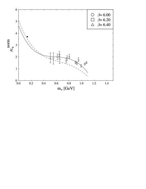
Figure 1: Lattice calculations for the isovector part of the a.m.m., $\kappa_{V}=\kappa_{p}-\kappa_{n}$ (experimental value: 3.71) as a function of the pion mass $m_{\pi}$. Full and dashed curves: predictions of ChPT with low-energy constants fitted to the lattice results. See Ref. Goe03 for further details .

3. COMPTON SCATTERING OF REAL PHOTONS AND THE HELICITY STRUCTURE OF PHOTOABSORPTION

3.1 Forward Dispersion Relations, Low Energy Theorems, and Sum Rules

In this section we discuss the forward scattering of a real photon by a nucleon. The incident photon is characterized by the Lorentz vectors of momentum, $q=(q_{0},\,\mathbf{q})$ and polarization, $\varepsilon_{\lambda}=(0,\,\bm{\varepsilon}_{\lambda})$, with $q\cdot q=0$ (real photon) and $\varepsilon_{\lambda}\cdot q=0$ (transverse gauge). If the photon moves in the direction of the $z$-axis, ${\mathbf{q}}=q_{0}\,{\hat{\mathbf{e}}}_{z}$, the two polarization vectors may be taken as

$$\bm{\varepsilon}_{\pm}=\mp\frac{1}{\sqrt{2}}\,(\hat{\mathbf{e}}_{x}\pm i\hat{\mathbf{e}}_{y})\ ,$$ (4)

corresponding to circularly polarized light with helicities $\lambda=+1$ (right-handed) and $\lambda=-1$ (left-handed). The kinematics of the outgoing photon is then described by the corresponding primed quantities. For the purpose of dispersion relations we choose the lab frame, and introduce the notation $q_{0}^{\mbox{\scriptsize{lab}}}=\nu$ for the photon energy. The absorption of this photon leads to an excited hadronic system with total c.m. energy $W=\sqrt{M^{2}+2M\nu}$.

The forward Compton amplitude takes the general form

$$T(\nu,\,\theta=0)=\bm{\varepsilon}^{\prime\ast}\cdot\bm{\varepsilon}\,f(\nu)+i\,\bm{\sigma}\cdot(\bm{\varepsilon}^{\prime\ast}\times\bm{\varepsilon})\,g(\nu)\ .$$ (5)

This amplitude is invariant under the crossing transformation, $\varepsilon^{\prime\ast}\leftrightarrow\varepsilon$ and $\nu\rightarrow-\nu$, and therefore $f$ has to be an even and $g$ an odd function of $\nu$. The amplitudes $f$ and $g$ can be determined by scattering circularly polarized photons (e.g., helicity $\lambda=1$) off nucleons polarized along or opposite to the photon momentum $\mathbf{q}$ as shown schematically in Fig. 2. If the spins are parallel, the helicity changes by two units and the intermediate state has helicity $3/2$. Since this requires a total spin $S\geq 3/2$, the transition can only take place on a correlated three-quark system. The case of opposite spins, on the other hand, is helicity conserving and therefore can take place on an individual quark. Denoting the Compton scattering amplitudes for these two experiments by $T_{3/2}$ and $T_{1/2}$, we find $f(\nu)=(T_{1/2}+T_{3/2})/2$ and $g(\nu)=(T_{1/2}-T_{3/2})/2$. In a similar way we define the total absorption cross section as the spin average over the two helicity cross sections,

$$\sigma_{T}=\frac{1}{2}\,(\sigma_{1/2}+\sigma_{3/2})\ ,$$ (6)

and the transverse-transverse interference term by the helicity difference,

$$\sigma_{TT}=\frac{1}{2}\,(\sigma_{1/2}-\sigma_{3/2})\ .$$ (7)

The unitarity of the scattering matrix relates the absorption cross sections to the imaginary parts of the respective forward scattering amplitudes by the optical theorem,

$$\mbox{Im}\ f(\nu) = \frac{\nu}{8\pi}(\sigma_{1/2}(\nu)+\sigma_{3/2}(\nu))=\frac{\nu}{4\pi}\,\sigma_{T}(\nu)\ ,$$

$$\mbox{Im}\ g(\nu) = \frac{\nu}{8\pi}(\sigma_{1/2}(\nu)-\sigma_{3/2}(\nu))=\frac{\nu}{4\pi}\,\sigma_{TT}(\nu)\ .$$ (8)

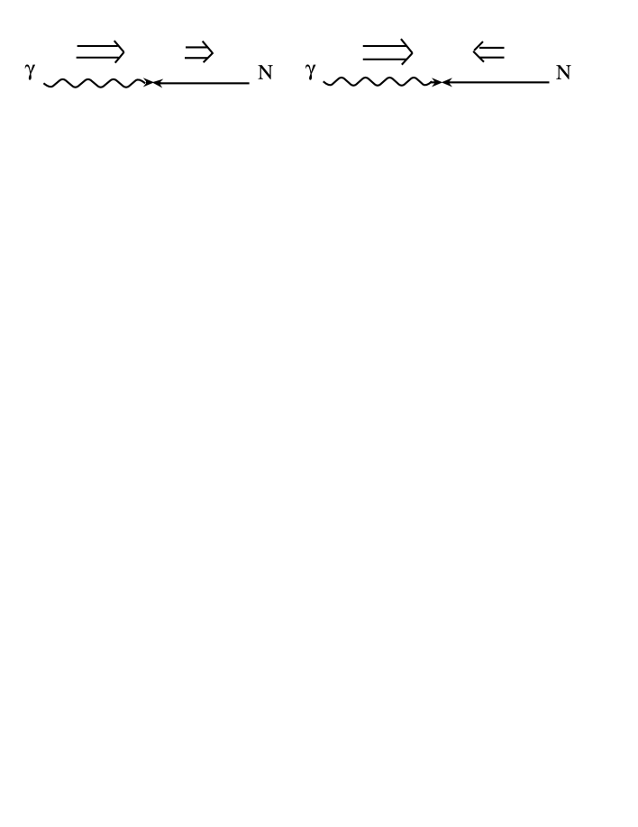
Figure 2: Spin and helicity of a double polarization experiment $\vec{\gamma}+\vec{N}\rightarrow N^{\ast}$. The open arrows denote the projections of the spin, $S_{z}$, on the photon momentum, the helicities $h$ are defined as projections on the respective particle momentum, and the photon is assumed to be right-handed (helicity $\lambda=+1$):
left: $N(S_{z}=1/2,\ h=-1/2)\rightarrow N^{\ast}(S_{z}=h=3/2)$,
right: $N(S_{z}=-1/2,\ h=1/2)\rightarrow N^{\ast}(S_{z}=h=1/2)$.

Due to the smallness of the fine structure constant $\alpha_{fs}$ we may neglect all purely electromagnetic processes, and shall consider only photoabsorption due to the hadronic channels starting at pion production threshold, $\nu_{0}=m_{\pi}(1+m_{\pi}/2M)\approx 150$ MeV. In order to set up the dispersion integrals, we have to study the behavior of the absorption cross sections for large energies. The total cross section $\sigma_{T}$ is essentially constant above the resonance region, with a slow logarithmic increase at the highest energies, and therefore we must subtract the dispersion relation for $f$. If we subtract at $\nu=0$, we also remove the nucleon pole terms at this point. By use of the crossing relation and the optical theorem, the subtracted dispersion relation takes the form,

$${\mbox{Re}}\ f(\nu)=f(0)+\frac{\nu^{2}}{2\pi^{2}}\,{\mathcal{P}}\,\int_{\nu_{0}}^{\infty}\,\frac{\sigma_{T}(\nu^{\prime})}{\nu^{\prime 2}-\nu^{2}}\,d\nu^{\prime}\ .$$ (9)

For the odd function $g(\nu)$ we may expect the existence of an unsubtracted dispersion relation,

$${\mbox{Re}}\ g(\nu)=\frac{\nu}{4\pi^{2}}\,{\mathcal{P}}\,\int_{\nu_{0}}^{\infty}\,\frac{\sigma_{1/2}(\nu^{\prime})-\sigma_{3/2}(\nu^{\prime})}{\nu^{\prime 2}-\nu^{2}}\,\nu^{\prime}d\nu^{\prime}\ .$$ (10)

If these integrals exist, they can be expanded in a Taylor series at the origin, which converges up to the lowest threshold, $\nu=\nu_{0}$ :

$${\mbox{Re}}\ f(\nu)\, = \,f(0)+\sum_{n=1}\left(\frac{1}{2\pi^{2}}\,\int_{\nu_{0}}^{\infty}\,\frac{\sigma_{T}(\nu^{\prime})}{\nu^{\prime 2n}}\,d\nu^{\prime}\right)\,\nu^{2n}\,,$$ (11)

$${\mbox{Re}}\ g(\nu)\, = \,\sum_{n=1}\left(\frac{1}{4\pi^{2}}\,\int\,\frac{\sigma_{1/2}(\nu^{\prime})-\sigma_{3/2}(\nu^{\prime})}{(\nu^{\prime})^{2n-1}}\,d\nu^{\prime}\right)\,\nu^{2n-1}\ .$$ (12)

The expansion coefficients in brackets parameterize the electromagnetic response of the nucleon.

The results of dispersion theory can be compared to the results of the low energy theorem (LET) of Low Low54 , and Gell-Mann & Goldberger Gel54 . These authors showed that the leading and next-to-leading terms of the expansions are fixed by the Born terms, which can be expressed by the global properties of the system, the mass $M$, the charge $e\,e_{N}$, and the a.m.m. $\kappa_{N}$ of the respective nucleon ($e_{p}=1,\ e_{n}=0,\ \kappa_{p}=1.79,\ \kappa_{n}=-1.91)$. Based on Lorentz invariance, gauge invariance and crossing symmetry, the LET yields the result

$$f(\nu) = -\frac{e^{2}\,e_{N}^{2}}{4\pi M}+(\alpha+\beta)\,\nu^{2}+{\mathcal{O}}(\nu^{4})\ ,$$ (13)

$$g(\nu) = -\frac{e^{2}\kappa^{2}_{N}}{8\pi M^{2}}\,\nu+\gamma_{0}\nu^{3}+{\mathcal{O}}(\nu^{5})\ .$$ (14)

The leading term of the spin-independent amplitude, $f(0)$, is the Thomson term familiar from nonrelativistic theory, and the term ${\mathcal{O}}(\nu)$ vanishes because of crossing symmetry. The term ${\mathcal{O}}(\nu^{2})$ describes Rayleigh scattering and yields information on the internal nucleon structure through the electric ($\alpha$) and magnetic ($\beta$) dipole polarizabilities, and the higher order terms ${\mathcal{O}}(\nu^{4})$ contain contributions of dipole retardation and higher multipoles. In the case of the spin-flip amplitude $g$, the leading term is determined by the a.m.m., and the term ${\mathcal{O}}(\nu^{3})$ contains information on the spin structure through the forward spin polarizability (FSP) $\gamma_{0}$. By comparing with Eqs. (11) and (12), we can construct all higher coefficients of the low energy expansion, Eqs. (13) and (14), from moments of the helicity cross sections. In particular we obtain Baldin’s sum rule Bal60 ,

$$\alpha+\beta=\frac{1}{2\pi^{2}}\,\int_{\nu_{0}}^{\infty}\,\frac{\sigma_{T}(\nu^{\prime})}{\nu^{\prime 2}}\,d\nu^{\prime}\ ,$$ (15)

the GDH sum rule Ger65 ,

$$\frac{\pi e^{2}\kappa^{2}_{N}}{2M^{2}}=\int_{\nu_{0}}^{\infty}\,\frac{\sigma_{3/2}(\nu^{\prime})-\sigma_{1/2}(\nu^{\prime})}{\nu^{\prime}}\,d\nu^{\prime}\,\equiv I\,,$$ (16)

and the FSP Gel54 ; GGT54 ,

$$\gamma_{0}=\,-\,\frac{1}{4\pi^{2}}\,\int_{\nu_{0}}^{\infty}\,\frac{\sigma_{3/2}(\nu^{\prime})-\sigma_{1/2}(\nu^{\prime})}{\nu^{\prime 3}}\,d\nu^{\prime}\ .$$ (17)

3.2 Photoabsorption Cross Sections for the Proton

The total photoabsorption cross section $\sigma_{T}$ for the proton is shown in Fig. 3. It clearly exhibits three resonance structures on top of a strong background. These structures correspond, in order, to concentrations of magnetic dipole strength $(M1)$ in the region of the $\Delta(1232)$ resonance, electric dipole strength $(E1)$ near the resonances $N^{\ast}(1520)$ and $N^{\ast}(1535)$, and electric quadrupole $(E2)$ strength near the $N^{\ast}(1680)$. For energies above the resonance region $(\nu\gtrsim 1.67$ GeV or $W\gtrsim 2$ GeV), $\sigma_{T}$ is slowly decreasing towards a minimum of $\sim 115~{}\mu$b at $W\approx 10$ GeV. At the highest energies, $W\approx 200$ GeV (corresponding to $\nu\simeq 2\cdot 10^{4}$ GeV), the experiments DESY show an increase with energy of the form $\sigma_{T}\sim W^{0.2}$, in accordance with Regge parametrizations through a soft pomeron exchange mechanism Cud00 . Although this increase is not expected to continue forever, we cannot expect that the unweighted integral over $\sigma_{T}$ converges, and therefore the dispersion relation for the spin-independent Compton amplitude $f$ has to be subtracted (see Eq. 9). In addition to the total cross section, Fig. 3 also shows the contributions of the most important channels. The one-pion channels dominate up to $\nu\approx 500$ MeV, but in the second resonance region ($\nu\approx 700$ MeV) the two-pion channels become quite comparable. The figure also shows the small contribution of $\eta$ production above $\nu\approx 700$ MeV.

Figure 3: The total absorption cross section $\sigma_{T}$ for the proton. The various lines represent the MAID results Maid03 for the total cross section (solid line), one-pion channels (dashed line), more-pion channels (dash-dotted line), and $\eta$ channel (dotted line). The data for the total cross section are from MAMI Mac96 (full circles) and Daresbury Dar72 (open circles). The triangles represent the data for the $2\pi$ channels Hol01 .

Recently, the helicity difference $\sigma_{TT}$ has also been measured. The first measurement was carried out at MAMI (Mainz) for photon energies in the range of 200 MeV$<\nu<800~{}$MeV Ahr00 , and the GDH Collaboration has now extended the measurement into the energy range up to 2.9 GeV at ELSA (Bonn) Dut03 . Further experimental activities in this range have been reported by groups at LEGS (Brookhaven) San02 , GRAAL (Grenoble) Bou02 , and SPring-8 (Hyogo) Iwa02 . As shown in Fig. 4, the helicity difference fluctuates much more strongly than the total cross section $\sigma_{T}$. The threshold region is dominated by s-wave pion production, i.e., intermediate states with spin $1/2$ that can only contribute to the cross section $\sigma_{1/2}$. In the region of the $\Delta(1232)$ with spin $J=3/2$, both helicity cross sections contribute, but since the transition is essentially $M1$, we find $\sigma_{3/2}/\sigma_{1/2}\approx 3$, and the helicity difference $\Delta\sigma=\sigma_{3/2}-\sigma_{1/2}=-2\sigma_{TT}$ becomes large and positive. The figure also shows that $\sigma_{3/2}$ dominates the proton photoabsorption cross section in the second and third resonance regions. In fact, one of the early successes of the quark model was to predict this feature by a cancellation of the convection and spin currents in the case of $\sigma_{1/2}$ Cop69 .

Figure 4: The helicity difference $\Delta\sigma=\sigma_{3/2}-\sigma_{1/2}$ for the proton. The various lines represent the results of MAID (for notation see Fig. 3). The experimental data are from MAMI Ahr00 (full circles) and ELSA Dut03 (open circles).

The preliminary data at the higher energies show some indication for the fourth resonance region (1800 MeV$<W<2000$ MeV) followed by a continuing decrease of $\Delta\sigma$ and a possible cross-over to negative values at $\nu\gtrsim 2.0$ GeV, as predicted from an extrapolation of DIS data Bia99 ; Sim02 . At high $\nu$, above the resonance region, one usually invokes Regge phenomenology to argue that the integral converges Bass97 . In particular, for the isovector channel $\sigma_{1/2}-\sigma_{3/2}$ behaves as $\nu^{\alpha_{V}-1}$ at large $\nu$, with $-0.5\lesssim\alpha_{V}\lesssim 0$ being the intercept of the $a_{1}(1260)$ meson Regge trajectory. For the isoscalar channel, Regge theory predicts a similar energy behavior with $\alpha_{S}\simeq-0.5$, which is the intercept of the isoscalar $f_{1}(1285)$ and $f_{1}(1420)$ Regge trajectories. However, these ideas should be tested experimentally.

We observe that the large background of non-resonant photoproduction in the total cross section $\sigma_{T}$ (Fig. 3) has almost disappeared in the helicity difference $\Delta\sigma$ (Fig. 4), i.e., the background is “helicity blind”. This is quite different from the behavior in the region of DIS, where helicity $3/2$ contributions should vanish relative to helicity $1/2$ contributions, because only the latter can be produced by incoherent scattering off a single quark. Obviously the transition from virtual photons to real photons can not be described by a simple extrapolation. The two helicity cross sections for real photons remain large and roughly equal up to the highest energies, at values of $\sigma_{1/2}\approx\sigma_{3/2}\approx 120~{}\mu$b. Therefore we conclude that the real photon is essentially absorbed by coherent processes. This absorption requires interactions among the constituents such as gluon exchange between two quarks.

3.2 The GDH Sum Rule for the Proton

The GDH sum rule predicts that the integral in Eq. (16) takes the value $I_{p}=204.8~{}\mu$b for the proton. As discussed above, the GDH sum rule is based on three very general principles (Lorentz and gauge invariance and unitarity) and on one weak assumption: the convergence of an unsubtracted dispersion relation. Although this assumption can never be proven or disproven by experiment, it is legitimate to ask whether the a.m.m. on the LHS of Eq. (16) is approximately obtained by integrating the measured cross sections up to some reasonable energy, say 3 or 50 GeV. This comparison will tell us whether the a.m.m. measured as a ground state expectation value, is related to the degrees of freedom visible to that energy, or whether it is produced by very short-distance and possibly still unknown phenomena, as we discussed in Section 1.

Let us therefore take a closer look at the different energy regions and their contributions to the GDH sum rule:

• The contributions for $0\leq\nu\leq\nu_{0}$, below the pion threshold, are only of electromagnetic origin and therefore of relative order $\kappa_{\rm{QED}}/\kappa_{p}\sim 10^{-3}$, where $\kappa_{\rm{QCD}}=\alpha_{fs}/(2\pi)$ is the Schwinger correction to the a.m.m. of the proton.

• The GDH experiments at MAMI and ELSA used longitudinally polarized protons provided by a frozen-spin butanol (C₄H₉OH) target. Although the (spinless) C and O atoms contained in this target should not affect the helicity difference, they give rise to large backgrounds for $\sigma_{1/2}$ and $\sigma_{3/2}$ separately. In order to obtain a good statistical accuracy, it is therefore a prerequisite to make sure the event happened on a target proton by detecting the emitted pions or the recoil proton under the right kinematical conditions. Of course such an experiment becomes increasingly difficult in the threshold region of $\nu<200$ MeV. However, the absorption cross sections in that region are completely dominated by the s- and p-wave multipoles, which are known from experimental analysis and are well described by ChPT and dispersion theory.

• The energy range of the MAMI experiment, 200 MeV$\leq\nu\leq 800$ MeV, includes the first and part of the second resonance region. The GDH Collaboration has extended the measurement of the helicity cross sections up to energies of $\nu=2.9$ GeV at ELSA, thus covering the full resonance region and very probably the onset of the Regge regime.

• The approved SLAC experiment E-159 E159 will measure the helicity difference $\Delta\sigma$ for protons and neutrons in the photon energy range of 5 GeV $<\nu<40$ GeV. The energy region of $2.5$ GeV$<\nu<5.5$ GeV was covered in a short run by the CLAS Collaboration at JLab Sob02 . The preliminary data indeed show a negative contribution of $\sim 4~{}\mu$b over that range, although this is much smaller than previously expected. The SLAC experiments will test the convergence of the GDH sum rule and provide a baseline for our understanding of soft Regge physics in the spin-dependent forward Compton amplitude.

Table 1 summarizes the results for the proton by showing predictions for the GDH integral and the FSP. The threshold contribution is evaluated by a multipole analysis of pion photoproduction Maid03 , with an error estimated by comparing to other analyses Arn02 . The resonance region up to $\nu=2.9$ GeV is determined by the experimental data taken at MAMI Ahr00 and ELSA Sch03 , and the asymptotic region is estimated from two different Regge analyses Bia99 ; Sim02 . Summing up these contributions, the GDH sum rule value is obtained within the error bars. Assuming that the estimated size of the Regge contribution will be confirmed by the proposed SLAC experiment E159, one may conclude that the GDH sum rule works for the proton. Because of the different energy weighting with $\nu$, the FSP integral converges much better and is therefore completely determined by the energy range of the existing data.

Table 1: The contribution of various energy regions to the GDH integral $I$ and the forward spin polarizability $\gamma_{0}$ of the proton (see text for explanation).

energy range	$I_{p}$ $[\mu$b]	$\gamma_{0}^{p}$ $[10^{-4}$0fm${}^{4}]$
$\nu_{0}\leq\nu\leq 200$0MeV0Maid03 ; Arn02	$-28.5\pm 2$	$0.95\pm 0.05$
200 MeV$\leq\nu\leq 800$0MeV0Ahr00	$226\pm 5\pm 12$	$-1.87\pm 0.08\pm 0.10$
800 MeV$\leq\nu\leq 2.9$0GeV0Sch03	$27.5\pm 2.0\pm 1.2$	$-0.03$
$\nu\geq 2.9$0GeV0Bia99 ; Sim02	$-14\pm 2$	$+0.01$
total	$211\pm 15$	$-0.94\pm 0.15$
sum rule0Ger65	204	–

3.4 The Helicity Structure of the Decay Channels

The cross sections $\Delta\sigma$ and $\sigma_{T}$ are divided into the contributions of the decay channels in Figs. 4 and 5. Up to the first resonance region the one-pion channels yield essentially all of the cross section. This changes in the second and third resonance regions, where the branching ratio for one-pion production, $x_{\pi}=\Gamma_{\pi}/\Gamma_{\rm{tot}}$, decreases to values near and below 50 %. Most of the remainder comes from the channels $\pi\pi$ and $\eta$. All other channels, including vector mesons ($\rho,\ \omega$) and strangeness production ($K\Lambda,\ K\Sigma$) yield only a small fraction of the GDH sum rule Zha02 . Table 2 gives a detailed break-down of the sum rule into the decay channels. The numbers in this table refer to the resonance region, $\nu\leq 1.67$ GeV or $W\leq 2$ GeV, except for the two-pion channels, for which no estimates exist above $\nu=800$ MeV. Also shown in Table 2 are the estimated asymptotic contributions for $\nu>1.67$ GeV. The table shows that the multipole analysis for one-pion production and the more phenomenological models for the heavier mass channels are in reasonable agreement with the sum rule in the case of the proton. However, the same analysis fails in the case of the neutron, which leaves an unexplained “gap” of $\sim 50~{}\mu$b between the model predictions and the sum rule.

Figure 5: Decay channels for photoabsorption on the proton according to various MAMI experiments. The data for total photoabsorption (open circles, Ref. Mac96 ) are compared to the following partial decay channels: $n\pi^{+}$ (solid and open triangles, Refs. Mac96 ; Ros04 ), $p\pi^{0}$ (diamonds, Ref. Har96 ), two-pion production (asterisks, Refs. Hol01 ), and $p\eta$ (squares, Ref. Kru95 ).

Table 2: The contribution of various decay channels to the GDH integral $I$ and the forward spin polarizability $\gamma_{0}$. The integration extends to $\nu_{\rm{max}}=1.67$ GeV ($W_{\rm{max}}=2$ GeV) except that the two-pion contribution is integrated only up to $\nu_{\rm{max}}=800$ MeV. The last row shows the results of Regge fits for the region $\nu>1.67$ GeV.

Ref.	proton	$I_{p}$	$\gamma_{0}^{p}$	neutron	$I_{n}$	$\gamma_{0}^{n}$
Maid03 /Arn02	$\pi^{0}p$	157/142	-1.46/-1.40	$\pi^{0}n$	145/147	-1.44/-1.44
Maid03 /Arn02	$\pi^{+}n$	7.5/44	0.82/0.55	$\pi^{-}p$	-21/-13	1.53/1.36
etaMaid	$\eta p$	-9.0	0.01	$\eta n$	-5.9	0.01
Hir02	$\pi\pi N$	$28$	$-0.07$	$\pi\pi N$	$19$	$-0.05$
Zha02	$K\Lambda,\ K\Sigma$	-4.0	$<0.01$	$K\Lambda,\ K\Sigma$	2.0	$<0.01$
Zha02	$\omega p,\ \rho N$	-3.0	$<0.01$	$\omega n,\ \rho N$	2.1	$<0.01$
Bia99 /Sim02	Regge	-25/-9	$<0.01$	Regge	31/16	$<0.01$

In the MAMI experiment on the proton, all decay channels were separately identified in the range of 200 MeV$<\nu<$800 MeV. Let us have a closer look at the contributing channels in order. For further details we refer the reader to a recent review by Krusche & Schadmand Kru03 .

One-pion channels: One-pion channels open at $\nu_{0}\approx 150$ MeV and dominate the cross section up to $\nu\approx 500$ MeV except for small contributions due to photonic decay of the excited states and the onset of two-pion production. Whereas the GDH integral receives substantial contributions also from heavier particles, the FSP is almost totally saturated at $\nu=800$ MeV. The helicity-dependent cross section for one-pion production may be expanded in the following multipole series Dre01 :

$$\sigma_{TT}(1\pi) = 4\pi\frac{k_{\pi}}{k_{\gamma}}\sum_{l}\frac{1}{2}(l+1)\left[(l+2)(|E_{l+}|^{2}+|M_{l+1,-}|^{2})\right.$$

$$\left.-l(|E_{l+1,-}|^{2}+|M_{l+}|^{2})+2l(l+2)\ \mbox{Re}\ (E_{l+}^{\ast}M_{l+}-E^{\ast}_{l+1,-}M_{l+1,-})\right]$$

$$= 4\pi\frac{k_{\pi}}{k_{\gamma}}\,(|E_{0+}|^{2}-|M_{1+}|^{2}+6\ \mbox{Re}\ (E_{1+}^{\ast}M_{1+})+3|E_{1+}|^{2}$$

$$+|M_{1^{-}}|^{2}-|E_{2-}|^{2}-6\ \mbox{Re}\ (E_{2-}^{\ast}M_{2-})+3|M_{2^{-}}|^{2}\pm\ ...)\ ,$$

where $k_{\pi}$ and $k_{\gamma}$ are the c.m. momenta of pion and photon, respectively. The electric (E) and magnetic (M) multipoles CGLN in this expansion are defined by the quantum numbers of the hadronic final state, with the first index ($\ell$) referring to the pion-nucleon orbital momentum and the second index ($\pm$) describing the coupling of orbital angular momentum and nucleon spin to the total angular momentum of the hadronic state ($J=\ell\pm\textstyle{\frac{1}{2}}$).

As we have seen, the threshold region was not covered by the experiment. The dominant multipole in this region is $E_{0+}$, which corresponds to an electric dipole (E1) transition leading to the production of (mostly charged) pions in an s wave. This multipole is well described by the analysis of (unpolarized) pion photoproduction in terms of angular distributions, ChPT Ber91 , dispersion theory Han98 , and phenomenological analysis Maid03 ; Arn02 . Also the onset of the p-wave multipoles seems to be well under control Ber95 .

With increasing photon energy, the first resonance becomes more and more dominant, mainly because of the magnetic dipole (M1) excitation of the $\Delta$ (1232), which is described by the multipole $M_{1+}$. The associated electric multipole $E_{1^{+}}$ corresponding to E2 excitation is strongly suppressed by the small ratio $R=E_{1^{+}}/M_{1^{+}}=(-2.5\pm 0.2\pm 0.2)$% as determined earlier by angular distributions and photon asymmetries for neutral pion photoproduction Bec97 . Because the product of these multipoles appears with a factor 6 in Eq. (3.4 The Helicity Structure of the Decay Channels), the “GDH experiment” allows for an independent measurement Ahr04 with the result $R=(-2.74\pm 0.03\pm 0.5)\%$. Altogether the MAMI data are in good agreement with the multipole analyses in the first resonance region Maid03 ; Arn02 , and also with the preliminary LEGS data San02 . However, even relatively small effects count in this region, because it provides the lion’s share to the sum rule, $I\,(\nu=250-400$ MeV$)=(176\pm 8)\,\mu$b!

The finite value of $E_{1^{+}}$ in the $N\rightarrow\Delta$ transition is evidence for tensor correlations, which may be attributed to the hyperfine interaction between the quarks due to gluon exchange. However, the bulk contribution to $E_{1^{+}}$ is found to stem from the pion cloud around the quark bag. From the negative value of $R$ one can derive, in the framework of various quark models, an oblate deformation of the $\Delta$ resonance.

In a similar way the $N\rightarrow N^{\ast}\,(1520)$ transition was studied by the GDH Collaboration Ahr02D . The multipoles $E_{2^{-}}$ and $M_{2^{-}}$ (E1 and M2 transitions, respectively) are related to the helicity amplitudes,

$$A_{1/2}\,(D_{13})\sim E_{2^{-}}-3M_{2^{-}}\ ,\quad A_{3/2}\,(D_{13})\sim\sqrt{3}(E_{2^{-}}+M_{2^{-}})\ .$$ (19)

The new results Ahr02D are $A_{1/2}=-38\pm 3$ (PDG, Ref. PDG : $-24\pm 9$) and $A_{3/2}=147\pm 10$ (PDG, Ref. PDG : $166\pm 5$), all in units of $10^{-3}$ GeV^-1/2. Expressed in terms of the multipoles, the ratio $M_{2^{-}}/E_{2^{-}}$ increases from 0.45 to 0.56, and the respective one-pion contribution to the sum rule decreases by $\sim 25$ %. From these examples it should become obvious that double-polarization experiments serve many purposes besides measuring the GDH integral. In particular, they provide a very sensitive tool to study resonance properties. For completeness we list the multipoles (in brackets: the electromagnetic transitions) of some other resonances. The Roper resonance $N^{\ast}\,(1440)$ with multipole $M_{1^{-}}(M1)$ contributes with the same sign as s-wave pion production, the $N^{\ast}\,(1535)$ appears as a resonance in the multipole $E_{0^{+}}(E1)$ just above $\eta$ threshold and dominates that decay process, and the most important resonance in the third resonance region is the $N^{\ast}\,(1680)$ with multipoles $E_{3^{-}}(E2)$ and $M_{3^{-}}(M3)$.

Two-pion channels: Although the reaction threshold lies in the $\Delta$ region at $\nu_{2\pi}=309$ MeV, this channel is practically absent below 400 MeV, and on the scale of Fig. 4 it becomes visible only for $\nu\gtrsim 500$ MeV. The interesting and previously unexpected feature is the peaking of the respective cross section at $\nu\approx 700$ MeV or $W\approx 1480$ MeV, definitely below the positions of the $D_{13}\ (1520)$ and $S_{11}\ (1535)$ resonances. This is experimental proof that two-pion production can not be simply explained by a resonance driven mechanism (s-channel contribution), but that it requires large non-resonant effects such as Born terms and vector meson exchange in the t-channel. The channels $n\pi^{+}\pi^{0}$, $p\pi^{+}\pi^{-}$, and $p\pi^{0}\pi^{0}$ were separately analyzed in the MAMI experiment Ahr03pipi . As an example we show the cross section for $\vec{\gamma}\vec{p}\rightarrow n\pi^{+}\pi^{0}$ in Figure 6. It leads to an important contribution of ($11.3\pm 0.7\pm 0.7)~{}\mu$b to the GDH integral in the range $\nu<800$ MeV, whereas its contribution changes the FSP by only $\sim 3$ %. Figure 6 demonstrates that the present models can only describe the data in a semi-quantitative way.

Figure 6: The total cross section $\sigma_{T}$ and the helicity difference $\Delta\sigma=\sigma_{3/2}-\sigma_{1/2}$ for the reaction $\vec{\gamma}\vec{p}\rightarrow n\pi^{+}\pi^{0}$. The theoretical predictions are shown by the solid lines Hir02 , dashed lines Nac02 , and dotted lines Hol01a . The data are from MAMI Ahr03pipi .

Eta channel: The $\eta$ channel provides another important contribution to the sum rule. If it were not for the mixing of the two particles, the $\eta\ (547)$ would be a member of the pseudoscalar meson octet and the $\eta^{\prime}\ (958)$ a member of the corresponding singlet. The latter acquires its large mass by the $U_{A}(1)$ anomaly, i.e., by its coupling to the gluon field. However, because the two particles have the same quantum numbers, the physical particles are superpositions of the pure octet and singlet states, and therefore the $\eta$ has a mass much larger than a typical Goldstone boson like the pion, whose mass would vanish in the limit of zero quark masses. The threshold for $\eta$ photoproduction is $\nu_{\eta}=706$ MeV. Etas are essentially produced by the decay of the nearby resonance $S_{11}\ (1535)$, which has an exceptionally large branching ratio of $\Gamma_{\eta}/\Gamma_{\rm{tot}}\lesssim 50$ %. This ratio is at most a few percent for all other resonances. Because the particle is pseudoscalar and the dominating resonance has $\ell=0$, this channel should essentially contribute to the helicity cross section $\sigma_{1/2}$ and the multipole $E_{0^{+}}$. This prediction was recently confirmed by a direct measurement at MAMI Ahr03eta in the $S_{11}\ (1535)$ resonance region. The result for $\sigma_{3/2}$ was compatible with zero, and $\sigma_{1/2}$ came out in perfect agreement with MAID etaMaid .

3.5 The GDH Sum Rule for the Neutron

Whereas experimental data support the existence of the GDH sum rule for the proton, the present situation is much less clear in the case of the neutron, for which the sum rule predicts the value $I_{n}=233.2\,\mu b$. From our knowledge of the CGLN multipoles and models of heavier mass intermediate states, we obtain ($129\pm 5)~{}\mu$b for the one-pion channel and $-6~{}\mu$b for $\eta$ production in the resonance region $W<2$ GeV (see also Table 2). An educated guess for two-pion production would be ($40\pm 20)~{}\mu$b, and the asymptotic contribution above 2 GeV has been estimated to yield another ($25\pm 10)~{}\mu$b. This estimate for $I_{n}$ falls short of the sum rule value by $\sim 20$ %. However, given the model assumptions and the uncertainties in the present data, one certainly cannot conclude that the neutron sum rule is violated. Possible sources of the discrepancy may be the neglect of final state interactions for pion production off the “neutron targets” ²H or ³He, the helicity structure of two-pion production, or the asymptotic contribution. Some of these open questions should be answered by the analysis of the data recently taken at ELSA and MAMI GDHneutron by the GDH collaboration.

Table 3: The magnetic moment $\mu$ (in units of $\mu_{N}$), the a.m.m. $\kappa$, and the GDH sum ${\rm{rule}}\ I$ (in units of $\mu$b) for electrons, protons, neutrons, deuterons, and ³He nuclei as well as fully polarized hydrogen atoms and butanol molecules.

	$e$	$p$	$n$	$d$	3He	1H	C4H9OH
$\mu$	-1838	2.793	-1.913	0.857	-2.128	-1836	-1.8$\cdot 10^{4}$
$\kappa$	$-1.2\cdot 10^{-3}$	1.793	-1.916	-0.143	-8.371	-918	-6.8$\cdot 10^{4}$
$I$	289	204.8	233.2	0.65	497.8	1.1$\cdot 10^{8}$	1.1$\cdot 10^{9}$

Table 3 shows the a.m.m. $\kappa$ for the nucleons and standard “neutron targets”. The most striking observation is the tiny value of $\kappa$ for the deuteron, a loosely bound system of a proton and a neutron, which has isospin $I=0$ and spin $S=1$ and is essentially in a relative s state. As a consequence the deuteron’s magnetic moment $\mu_{d}$ is roughly the sum of $\mu_{p}$ and $\mu_{n}$, the large isovector component of the nucleon magnetic moments cancels, and the result is $\mu_{d}\approx\mu_{N}$. As can be seen from Eq. (2), the “normal” magnetic moment of the deuteron takes exactly the same value and therefore $\kappa_{d}\ll 1$ and $I_{d}\ll I_{p}+I_{n}$. The large contributions of the subnuclear degrees of freedom above pion threshold have to be cancelled by contributions of the nuclear degrees of freedom, and this must happen to three decimal places!

Let us now apply the same reasoning to ³He, a system of two protons with spins paired off and an “active” neutron, essentially again in s states of relative motion. The result is that $\mu_{{}^{3}\rm{He}}\approx\mu_{n}<0$, whereas, according to Eq. (2), the “normal” moment of ³He takes a positive value. As a consequence $\kappa_{{}^{3}\rm{He}}$ has a large negative value, and $I_{{}^{3}\rm{He}}$ is much larger than in the deuteron case.

Arenhövel and collaborators have investigated the interplay between nuclear and subnuclear degrees of freedom for the deuteron Are97 . They begin with a nonrelativistic potential model approach but include meson exchange and isobar currents as well as relativistic corrections. The most important channel is deuteron disintegration, $\gamma+d\rightarrow p+n$, which yields a maximum value of $\sigma_{P}-\sigma_{A}\approx-1800~{}\mu$b at $\nu\approx 2.3$ MeV owing to the M1 transition ${}^{3}S_{1}\rightarrow{}^{1}S_{0}$. Note that this nuclear transition changes the magnetic moments of the constituents from parallel to antiparallel. To the contrary, the $N\rightarrow\Delta$ transition leads to a parallel orientation of all quark spins and peaks at $\nu\approx 330$ MeV with a maximum value of $\sigma_{P}-\sigma_{A}\approx+700~{}\mu$b. As a function of $\nu_{\rm{max}}$, the upper limit of integration, the disintegration channel yields the following contributions to the GDH sum rule: $I_{\rm{pn}}\,(10~{}\rm{MeV})\approx-600~{}\mu$b, $I_{\rm{pn}}\,(150~{}\rm{MeV})\approx-510~{}\mu$b, and $I_{\rm{pn}}\,(550~{}\rm{MeV})\approx-413~{}\mu$b. This channel seems to be saturated at 550 MeV, which also marks the limit of a nonrelativistic calculation. Coherent pion production gives another important contribution, $I_{\pi^{0}d}\,(550~{}\rm{MeV})=63~{}\mu$b. In total the calculation yields $-350~{}\mu$b from these two coherent processes. The contributions of incoherent production of pions and heavier mass systems, as estimated from the free nucleons, yield $I_{p}+I_{n}=438~{}\mu$b. As a result the cancellation of nuclear and subnuclear contributions is indeed large, but not large enough to reach the extremely small value of $I_{d}$.

Eagerly waiting for the results of the ELSA and MAMI experiments on the deuteron target, we can only speculate about the open questions:

• A first glimpse of the reaction $\vec{\gamma}+\vec{d}\rightarrow\pi^{-}+p+p_{\rm{spectator}}$ gives the impression that final state scattering is small, and that the impulse approximation may be an adequate treatment Ped04 . Although this leads to some reduction in the $\Delta$ region, the overall change of the sum rule contribution by binding effects is probably small. However, a 20 % reduction of the incoherent contribution would be necessary to reach the small value of $I_{d}$.

• The positive contributions of the two coherent processes around $\nu=300$ MeV are certainly driven by photo-excitation of the $\Delta$ resonance with the decay pion being reabsorbed by the spectator nucleon. On the other hand the nearby possibility of pion photoproduction will also be felt in the photodisintegration process below threshold. Nuclear and subnuclear degrees of freedom are thus deeply interwoven.

• Relativistic corrections Are97 decrease $I_{pn}$ from $-619~{}\mu$b to $-413~{}\mu$b, which may indicate the need for a truly Lorentz invariant description. In spite of such possible shortcomings, the non-relativistic calculation fulfills an interesting relation in the limit $\kappa_{p,n}\rightarrow 0$: The contribution of deuteron breakup, $I_{pn}$, tends to zero as is required for consistency, because also the contributions of pion photoproduction vanish in that limit.

• On the basis of the existing calculations, the simple recipe to derive $I_{n}$ from the inclusive helicity cross sections above pion threshold is bound to fail. We also run into serious conceptual problems if we somehow subtract the coherent processes above that threshold or divide them between the nucleons and the nucleus. The only real hope for a quantitative solution of the neutron puzzle is that the final data analysis might essentially confirm the validity of the impulse approximation for incoherent pion production. By correcting for Fermi motion effects, it may then be possible to derive the helicity cross sections for the free neutron from the experimental values, with the additional check that this procedure should also work for the proton.

Concerning the ³He target, the ongoing electroproduction experiments at JLab (see Section 4) are presently analyzed within the impulse approximation and including a (small) depolarization factor due to the probability of relative d states in ³He. Because the proton spins are paired off and the impulse approximation leads only to small modifications for the polarized neutron, the inclusive helicity difference above pion threshold is then assumed to yield $I_{n}$ modulo the corrections for Fermi motion. As a result the nuclear effects below pion threshold should yield a contribution of $\sim 260~{}\mu$b in order to fulfill the sum rule for ³He. However, this procedure can only yield a first estimate, because non-pionic breakup and coherent pion production (³He $\pi^{0}$ and ³H $\pi^{+}$ final states!) will certainly complicate the analysis.

As we stated above, the interplay of nuclear and subnuclear degrees of freedom is based on the general principles that enter the low-energy theorems and dispersion relations. A complete answer to the questions arising in this context calls for experiments over the full energy range. It is therefore very promising that programs are also developing for energies between nuclear breakup and pion threshold at TUNL/HI$\gamma$S (Duke) TUNL , both for the nuclear physics aspects by themselves and as a test of many-body calculations that inevitably will be required to determine whether the GDH sum rule is fulfilled for the neutron.

We conclude this subsection with a possibly academic but still interesting question. Although we have talked about nucleons and nuclei as targets, we could just as well think about projects to measure the GDH sum rule for atoms or molecules. Table 3 shows the a.m.m. $\kappa$ and the GDH sum rule $I$ for several such systems. The comparison of the different hierarchies is quite amusing. If one tried to reconstruct, for example, the a.m.m. of the hydrogen atom by a GDH integral over its atomic spectrum in the eV or keV region, one would find physics “beyond”: the physics of $e^{+}e^{-}$ pair production at the MeV scale (QED) and hadronic physics above pion threshold (QCD).

3.6 Predictions for the Spin Polarizabilities

Because the GDH sum rule involves the magnetic moment, ChPT can not predict the sum rule but tacitly assumes its validity by inserting the appropriate LECs. However, there are genuine predictions for the polarizabilities and in particular also for the FSP. The first calculation of Compton scattering in ChPT was performed by Bernard et al. in 1991 BKM91 . Keeping only the leading term at order $p^{3}$ they obtained the result

$$\alpha=10\beta=\frac{5\alpha_{fs}g_{A}^{2}}{96\pi f_{\pi}^{2}m_{\pi}}=12.2\cdot 10^{-4}~{}{\rm{fm}}^{2}\ ,$$ (20)

in remarkable agreement with experiment (see Ref. Olm01 and references cited therein). The calculation was later repeated in heavy baryon ChPT, which allows for a consistent chiral power counting, and extended to ${\mathcal{O}}(p^{4})$. At that order there appear several LECs, which were determined by resonance saturation BKSM93 , i.e., by putting in phenomenological information about the $\Delta$ (1232) resonance. Because this resonance lies close by, it may not be justifiable to “freeze” its degrees of freedom. It was therefore proposed HHK97 to include the excitation energy of the $\Delta$ (1232) by means of an additional expansion parameter (“$\varepsilon$ expansion”). Unfortunately, at ${\mathcal{O}}(\varepsilon^{3})$ the “dynamical” $\Delta$ increases the polarizabilities to values far above the data. Since large loop corrections are expected at ${\mathcal{O}}(\varepsilon^{4})$, a calculation to this order might remedy the situation. Otherwise one would have to shift the problem to large contributions of counter terms, thus losing the predictive power.

Table 4: Theoretical predictions for the forward spin polarizability of the proton and neutron in units of $10^{-4}$ fm⁴. The table contains the results of heavy baryon ChPT at ${\mathcal{O}}(p^{3})$ BKKM92 and ${\mathcal{O}}(p^{4})$ Kum00 , the small scale expansion HHKK98 , the full one-loop result (not expanded!) of Lorentz-invariant baryon ChPT Ber03 , fixed-$t$ dispersion relation DPV03 ; Bab98a , hyperbolic dispersion relations DPV03 , a dressed K-matrix model KS01 and the hypercentral quark model Gor04 .

Ref.	BKKM92	Kum00	HHKK98	Ber03	DPV03	Bab98a	DPV03	KS01	Gor04
$\gamma_{0}^{p}$	4.6	-3.9	2.0	4.6	-0.7	-1.5	-1.1	2.4	-1.0
$\gamma_{0}^{n}$	4.6	-0.7	2.0	1.8	-0.07	0.4	-0.5	2.0	-1.1

The spin polarizabilities were first predicted in heavy baryon ChPT BKKM92 at ${\mathcal{O}}(p^{3})$. Two later calculations Kum00 at ${\mathcal{O}}(p^{4})$ yielded the result

$$\gamma_{0}^{p} = \frac{\alpha_{fs}g_{A}^{2}}{24\pi^{2}f_{\pi}^{2}m_{\pi}^{2}}\left(1-\frac{\pi m_{\pi}}{8M}(21+4\kappa_{p}-2\kappa_{n})\right)$$ (21)

$$= (4.5-8.3)\cdot 10^{-4}\,fm^{-4}=-3.8\cdot 10^{-4}\,fm^{-4}\ .$$

This calculation was recently repeated within a newly developed Lorentz-invariant formulation of baryon ChPT Ber03 . The full one-loop result, expanded as a power series in $m_{\pi}$, takes the form $\gamma_{0}^{p}=4.5-8.3+6.0+3.2+{\mathcal{O}}(m_{\pi}^{2})=4.6$ (in units of $10^{-4}$ fm^-4). The leading and subleading terms agree, of course, with Eq. (21). However, the following terms indicate that the expansion does not seem to converge to the experimental result of Table 2. Equation (21) shows that the bad convergence is due to unexpectedly large prefactors of the expansion parameter $m_{\pi}/M\approx 1/7$. As has been pointed out, this problem is essentially due to the Born terms Ber03 . However, we will have to wait for a full two-loop calculation (and possibly for the inclusion of the “dynamical” $\Delta$), before we can draw definite conclusions about the convergence of the FSP as a function of $m_{\pi}$.

Table 4 lists several predictions for the FSP. For more details about the polarizabilities of the nucleon, we refer the reader to Ref. DPV03 and several recent investigations including the $\Delta(1232)$ as an explicit degree of freedom Ber03 ; Hil03 . Finally we would like to mention that the first predictions of lattice QCD have recently appeared latticepol , though as yet only for the scalar polarizabilities $\alpha$ and $\beta$ and pion masses above 550 MeV.

4. DOUBLY-VIRTUAL COMPTON SCATTERING AND GENERALIZED GDH INTEGRALS

4.1 VVCS and Inclusive Lepton Scattering

In this section we consider the forward scattering of a virtual photon with space-like four-momentum $q$, i.e., $q^{2}=q^{2}_{0}-{\mathbf{q}}^{2}=-Q^{2}<0$. This doubly-virtual Compton scattering (VVCS) offers a useful framework to study the generalized GDH integrals and polarizabilities Ji93 . However, it is not merely a theoretical construct. As pointed out many years ago Ruj71 , the imaginary part of this amplitude can be studied by measuring the (transverse) vector analyzing power or single spin asymmetry (SSA) in elastic lepton scattering. The SSA is parity conserving but time-reversal odd, and therefore it vanishes in first-order perturbation theory. As a result the measured asymmetry is determined by the product of the (real) Born amplitude for one-photon exchange with the imaginary part of two-photon exchange, which is of course given by the VVCS tensor. A pioneering experiment to measure the SSA has been performed at MIT/Bates Wel01 , and more data are expected from ongoing or proposed experiments at the JLab Kum99 , SLAC Kum04 , and MAMI Maa04 . The SSA has also been discussed in the context of deeply virtual Compton scattering for the transition from a space-like to a time-like photon, which offers the possibility to study generalized parton distributions Gui03 .

The absorption of a virtual photon on a nucleon $N$, is related to inclusive electroproduction, $e+N\rightarrow e^{\prime}+$ anything, where $e$ and $e^{\prime}$ are the electrons in the initial and final states, respectively. The kinematics of the electron is traditionally described in the lab frame (rest frame of $N$), with $E$ and $E^{{}^{\prime}}$ denoting the initial and final energies of the electron, respectively, and $\theta$ the scattering angle. This defines the kinematics of the virtual photon in terms of four-momentum transfer $Q$ and energy transfer $\nu$,

$$Q^{2}=4EE^{{}^{\prime}}\sin^{2}\frac{\theta}{2},\quad\nu=E-E^{{}^{\prime}}\ .$$ (22)

In the c.m. frame of the hadronic intermediate state, the four-momentum of the virtual photon is given by

$$\omega_{\gamma}=\frac{M\nu-Q^{2}}{W},\quad{\mathbf{k}}_{\gamma}=\frac{M}{W}\,{\mathbf{q}}\ ,$$ (23)

where $|{\mathbf{q}}|=\sqrt{Q^{2}+\nu^{2}}$ is the lab photon momentum and $W=\sqrt{2M\nu+M^{2}-Q^{2}}$ the total energy in the hadronic c.m. frame. We also introduce the Bjorken variable $x=Q^{2}/2M\nu$. The virtual photon spectrum is normalized according to Hand’s definition Han63 by the “equivalent photon energy” $K=K_{H}=\nu(1-x)=(W^{2}-M^{2})/2M$. This replaces the photon energy, which according to Eq. (23) vanishes in the c.m. frame at $\nu=Q^{2}/M$ and therefore is inconvenient in the context of the multipole expansion. However, an alternative would be Gilman’s definition Gil68 , $K_{G}=|{\mathbf{q}}|$.

The inclusive inelastic cross section may be written in terms of a flux factor and four partial cross sections Dre01 ,

$$\frac{d\sigma}{d\Omega\ dE^{\prime}}=\Gamma_{V}\sigma(\nu,Q^{2})\ ,$$ (24)

$$\sigma=\sigma_{T}+\epsilon\sigma_{L}-hP_{x}\sqrt{2\epsilon(1-\epsilon)}\ \sigma_{LT}-hP_{z}\sqrt{1-\epsilon^{2}}\ \sigma_{TT}\ ,$$ (25)

with the photon polarization $\epsilon$ and the virtual photon flux factor $\Gamma_{V}$,

$$\epsilon=\frac{1}{1+2(1+\nu^{2}/Q^{2})\tan^{2}\theta/2}\ ,\quad\Gamma_{V}=\frac{\alpha_{fs}}{2\pi^{2}}\ \frac{E^{\prime}}{E}\ \frac{K}{Q^{2}}\ \frac{1}{1-\epsilon}\ .$$ (26)

In addition to the transverse ($\sigma_{T}$) and longitudinal ($\sigma_{L}$) cross sections, the polarization of the virtual photon gives rise to longitudinal-transverse ($\sigma_{LT}$) and transverse-transverse ($\sigma_{TT}$) interference terms. The two spin-flip (interference) cross sections can only be measured by a double-polarization experiment, in which $h=\pm 1$ refers to the two helicity states of the (relativistic) electron, and $P_{z}$ and $P_{x}$ denote the components of the target polarization in the direction of the virtual photon momentum ${\mathbf{q}}$ and perpendicular to that direction in the scattering plane of the electron. Contrary to the sign convention of Reference Dre01 , we have followed the standard notation of DIS: $\sigma_{LT/TT}$ (Equation 25) $=-\sigma^{\prime}_{LT/TT}$ (Reference Dre01 ).

The spin-flip cross sections are related to the quark structure functions $g_{1}$ and $g_{2}$ as follows DPV03 :

$$\sigma_{TT}=\displaystyle{\frac{4\pi^{2}\alpha_{fs}}{MK}}\left(g_{1}-\gamma^{2}\,g_{2}\right)\ ,\quad\sigma_{LT}=\displaystyle{\frac{4\pi^{2}\alpha_{fs}}{MK}}\,\gamma\,\left(g_{1}+g_{2}\right)\ ,$$ (27)

with $\gamma=Q/\nu$. The one-pion contribution to these cross sections may be expressed in terms of the electric (E), magnetic (M), and Coulomb or “scalar” (S) multipoles,

$$\sigma_{TT}^{(1\pi)} = 4\pi\frac{k_{\pi}}{K_{W}}\sum_{l}\frac{1}{2}(l+1)\left[(l+2)(|E_{l+}|^{2}+|M_{l+1,-}|^{2})\right.$$

$$\left.-l(|E_{l+1,-}|^{2}+|M_{l+}|^{2})+2l(l+2){\rm{Re}}(E_{l+}^{\ast}M_{l+}-E^{\ast}_{l+1,-}M_{l+1,-})\right]\ ,$$

$$\sigma_{LT}^{(1\pi)} = 4\pi\frac{k_{\pi}}{K_{W}}\frac{Q}{k_{\gamma}}\sum_{l}\frac{1}{2}(l+1)^{2}$$

$$\cdot{\rm{Re}}\left[S_{l+}^{\ast}((l+2)E_{l+}+lM_{l+})+S_{l+1,-}^{\ast}(lE_{l+1,-}-(l+2)M_{l+1,-})\right]\ ,$$

with $K_{W}=\frac{M}{W}K$, and $k_{\pi}$ and $k_{\gamma}$ the c.m. momenta of pion and photon, respectively.

The VVCS amplitude for forward scattering of virtual photons generalizes Eqs. (4) and (5) by introducing an additional longitudinal polarization vector $\hat{\mathbf{q}}$,

$$T(\nu,\,Q^{2},\,\theta=0) \;=\; {\bm{\varepsilon}}\,^{\prime\ast}\cdot{\bm{\varepsilon}}\,f_{T}(\nu,\,Q^{2})\;+\;f_{L}(\nu,\,Q^{2})$$ (30)

$$+ \;i{\bm{\sigma}}\cdot({\bm{\varepsilon}}\,^{\prime\ast}\times{\bm{\varepsilon}})\,g_{TT}(\nu,\,Q^{2})$$

$$+ i\,({\bm{\varepsilon}}\,^{\prime\ast}-{\bm{\varepsilon}})\cdot({\bm{\sigma}}\times\hat{\mathbf{q}}\,)\,g_{LT}(\nu,\,Q^{2})\ .$$

In order to construct the VVCS amplitudes in one-to-one correspondence with the nucleon structure functions, it is useful to cast Eq. (30) in a covariant form,

$$T(\nu,\,Q^{2},\,\theta=0)\;=\;\varepsilon_{\mu}^{\prime\ast}\varepsilon_{\nu} \left\{\left(-g^{\mu\nu}+\frac{q^{\mu}q^{\nu}}{q^{2}}\right)T_{1}(\nu,\,Q^{2})\right.$$ (31)

$$\left.+\frac{1}{p\cdot q}\left(p^{\mu}-\frac{p\cdot q}{q^{2}}\,q^{\mu}\right)\left(p^{\nu}-\frac{p\cdot q}{q^{2}}\,q^{\nu}\right)T_{2}(\nu,\,Q^{2})\right.$$

$$\left.+\frac{i}{M}\,\epsilon^{\mu\nu\alpha\beta}\,q_{\alpha}s_{\beta}\,S_{1}(\nu,\,Q^{2})\right.$$

$$\left.+\frac{i}{M^{3}}\,\epsilon^{\mu\nu\alpha\beta}\,q_{\alpha}(p\cdot q\ s_{\beta}-s\cdot q\ p_{\beta})\,S_{2}(\nu,\,Q^{2})\right\}\,,$$

where $\epsilon_{0123}=+1$, $p$ is the nucleon momentum, and $s$ is the nucleon covariant spin vector that satisfies $s\cdot p=0$ and $s^{2}=-1$. In the following we are concerned only with the spin-dependent structure functions of Eqs. (30) and (31), which are related by

$$S_{1}(\nu,\,Q^{2}) = \frac{\nu\,M}{\nu^{2}+Q^{2}}\left(g_{TT}(\nu,\,Q^{2})+\frac{Q}{\nu}\,g_{LT}(\nu,\,Q^{2})\right)\,,$$

$$S_{2}(\nu,\,Q^{2}) = -\frac{M^{2}}{\nu^{2}+Q^{2}}\left(g_{TT}(\nu,\,Q^{2})-\frac{\nu}{Q}\,g_{LT}(\nu,\,Q^{2})\right)\,.$$ (32)

As in the case of real Compton scattering, the VVCS amplitude has to be symmetric under the crossing operation, i.e., under the replacements $\varepsilon_{\mu}^{\prime\ast}\leftrightarrow\varepsilon_{\mu}$, $q_{\mu}\rightarrow-q_{\mu}$, and in particular for $\nu=p\cdot q/M\rightarrow-\nu$. An inspection of Eqs. (30) and (31) therefore yields the results

$$\begin{array}[]{lllllll}S_{1}(\nu,Q^{2})&=&S_{1}(-\nu,Q^{2})\ ,&S_{2}(\nu,Q^{2})&=&-S_{2}(-\nu,Q^{2})\ ,\\ g_{TT}(\nu,Q^{2})&=&-g_{TT}(-\nu,Q^{2})\ ,&g_{LT}(\nu,Q^{2})&=&g_{LT}(-\nu,Q^{2})\ .\end{array}$$ (33)

4.2 Dispersion Relations and Sum Rules

In order to set up dispersion relations, we have to construct the imaginary parts of the amplitudes with contributions from both elastic and inelastic scattering. The elastic contributions are obtained from the direct and crossed Born diagrams with the usual form of the electromagnetic vertex for the transition $\gamma^{*}(q)+N(p)\to N(p+q)$,

$$\Gamma^{\mu}\;=\;F_{D}(Q^{2})\,\gamma^{\mu}\;+\;F_{P}(Q^{2})\,i\sigma^{\mu\nu}\frac{q_{\nu}}{2M}\;,$$ (34)

with $F_{D}$ and $F_{P}$ denoting the nucleon Dirac and Pauli form factors, respectively. The straightforward calculation yields the result DPV03

$$g_{TT}^{\mbox{\scriptsize{Born}}}(\nu,\,Q^{2}) = -\frac{\alpha_{fs}\nu}{2M^{2}}\left(F_{P}^{2}+\frac{Q^{2}}{\nu^{2}-\nu_{B}^{2}+i\varepsilon}\,G_{M}^{2}\right)\,,$$

$$g_{LT}^{\mbox{\scriptsize{Born}}}(\nu,\,Q^{2}) = \frac{\alpha_{fs}Q}{2M^{2}}\left(F_{D}F_{P}-\frac{Q^{2}}{\nu^{2}-\nu_{B}^{2}+i\varepsilon}\,G_{E}G_{M}\right)\,,$$ (35)

where $\nu_{B}=Q^{2}/2M$. We have split the elastic amplitudes of Eq. (4.2 Dispersion Relations and Sum Rules) into a real contribution and a complex one containing the electric and magnetic Sachs form factors $G_{E}\,(Q^{2})=F_{D}\,(Q^{2})-\tau\,F_{P}(Q^{2})\ ,\quad G_{M}\,(Q^{2})=F_{D}\,(Q^{2})+F_{P}(Q^{2})$, with $\tau=Q^{2}/4M^{2}$. These form factors are normalized to $G_{E}(0)=e_{N}\ ,\quad G_{M}(0)=e_{N}+\kappa_{N}$, where $e_{N}$ and $\kappa_{N}$ are the charge (in units of $e$) and the a.m.m. of the respective nucleon. We also note that perturbative QCD predicts $F_{D}(Q^{2})\sim Q^{-4}$ and $F_{P}(Q^{2})\sim Q^{-6}$ if $Q^{2}\rightarrow\infty$.

Equation (4.2 Dispersion Relations and Sum Rules) shows us that the transition from real to virtual photons is not straightforward, because the limits $Q^{2}\rightarrow 0$ and $\nu\rightarrow 0$ cannot be interchanged Ji93 . The Born amplitudes of VVCS have poles at $\nu=\pm\nu_{B}\mp i\varepsilon$, corresponding to s- and u-channel elastic scattering. In particular, the amplitudes are complex at this pole, because the virtual photon can be absorbed at $\nu=\nu_{B}=Q^{2}/2M$ or $x=1$.

In more physical terms, the crucial difference between a (space-like) virtual and a real photon is the fact that the former can be absorbed by a charged particle whereas the latter can only be “absorbed” at zero frequency, $\nu=0$. At this point the real photon amplitudes can be expanded in a Taylor series whose leading terms are determined by the Born terms; in particular, $g_{TT}^{\rm{Born}}(\nu,0)$ reproduces exactly the leading term of the spin-flip amplitude $g(\nu)$ of Eq. (14). The GDH sum rule is then obtained by equating that series to an expansion of the dispersion integral that involves imaginary parts from the inelastic processes for $\nu>\nu_{0}$. The case of a virtual photon differs in two aspects: The imaginary parts stem from both inelastic and elastic processes, and the real parts of the amplitudes have two poles in the $\nu$ plane.

The inelastic contributions are regular functions in the complex $\nu$-plane except for cuts from $-\infty$ to $-\nu_{0}$ and $+\nu_{0}$ to $+\infty$. The optical theorem relates the inelastic contributions to the partial cross sections of inclusive electroproduction,

$${\mbox{Im}}\ g_{TT}(\nu,\,Q^{2})=\frac{K}{4\pi}\sigma_{TT}(\nu,\,Q^{2})\ ,\qquad{\mbox{Im}}\ g_{LT}(\nu,\,Q^{2})=\frac{K}{4\pi}\sigma_{LT}(\nu,\,Q^{2})\ ,$$ (36)

for energies above pion threshold, $\nu>\nu_{0}=m_{\pi}+(m_{\pi}^{2}+Q^{2})/2M$. We note that the products $K\,\sigma_{TT/LT}$ are independent of the choice of $K$, because they are directly proportional to the measured cross section (see Eqs. (24)$-$(26)). Of course, the natural choice at this point would be $K=K_{G}=|{\mathbf{q}}|$, because we expect the photon three-momentum on the RHS of Eq. (36). However, for reasons explained above, we have chosen $K=K_{H}$.

The imaginary parts of the relativistic spin amplitudes follow from Eqs. (4.1 VVCS and Inclusive Lepton Scattering) and (36),

$${\rm Im}\ S_{1} = \frac{\nu\,M}{\nu^{2}+Q^{2}}\,\frac{K}{4\pi}\,\left(\sigma_{TT}+\frac{Q}{\nu}\,\sigma_{LT}\right)=\frac{e^{2}}{4M}\,\frac{M}{\nu}\,g_{1}\ ,$$

$${\rm Im}\ S_{2} = -\frac{M^{2}}{\nu^{2}+Q^{2}}\,\frac{K}{4\pi}\,\left(\sigma_{TT}-\frac{\nu}{Q}\,\sigma_{LT}\right)=\frac{e^{2}}{4M}\,\frac{M^{2}}{\nu^{2}}\,g_{2}\ .$$ (37)

As was pointed out in Ref. DPV03 , this definition does not contain a singularity at $\nu=\pm iQ$, because this point corresponds to the Siegert limit, where $\sigma_{TT}=\pm i\sigma_{LT}$.

We next turn to the sum rules for the spin dependent VVCS amplitudes (see also Ref. JiO01 and references therein). Assuming an appropriate high-energy behavior, the spin-flip amplitude $g_{TT}$ (which is odd in $\nu$) satisfies an unsubtracted dispersion relation as in Eq. (10),

$${\mbox{Re}}\ g_{TT}\,(\nu,\,Q^{2})=\frac{2\nu}{\pi}\,{\mathcal{P}}\,\int_{0}^{\infty}\,\frac{{\mbox{Im}}\ g_{TT}\,(\nu^{\prime},\,Q^{2})}{\nu^{\prime 2}-\nu^{2}}\,d\nu^{\prime}\ .$$ (38)

Separating the contributions of the elastic scattering at $\nu^{\prime}=\nu_{B}$ from the inelastic contribution at $\nu^{\prime}>\nu_{0}$ as given by Eq. (36), we obtain :

$${\mbox{Re}}\left[\ g_{TT}\,(\nu,Q^{2})-g_{TT}^{\mbox{\scriptsize{pole}}}(\nu,Q^{2})\right] = \frac{\nu}{2\pi^{2}}\,{\mathcal{P}}\int_{\nu_{0}}^{\infty}\frac{K(\nu^{\prime},Q^{2})\,\sigma_{TT}(\nu^{\prime},Q^{2})}{\nu^{\prime 2}-\nu^{2}}\,d\nu^{\prime}$$

$$= \frac{2\,\alpha_{fs}}{M^{2}}\,I_{TT}(Q^{2})\;\nu+\gamma_{TT}(Q^{2})\;\nu^{3}+{\mathcal{O}}(\nu^{5})\,.$$

Because the RHS of this equation is now a regular function, it can be expanded in a Taylor series whose leading terms yield a generalization of the GDH sum rule,

$$I_{TT}(Q^{2}) = \frac{M^{2}}{\pi\,e^{2}}\,\int_{\nu_{0}}^{\infty}\,\frac{K(\nu,\,Q^{2})}{\nu}\,\frac{\sigma_{TT}\,(\nu,\,Q^{2})}{\nu}\,d\nu\,,$$ (40)

$$= \frac{2\,M^{2}}{Q^{2}}\,\int_{0}^{x_{0}}\,dx\,\left\{g_{1}\,(x,\,Q^{2})-\frac{4M^{2}}{Q^{2}}\,x^{2}\,g_{2}\,(x,\,Q^{2})\right\}\,,$$

and similarly a generalized form of the FSP,

$$\gamma_{TT}\,(Q^{2}) = \frac{1}{2\pi^{2}}\,\int_{\nu_{0}}^{\infty}\,\frac{K(\nu,\,Q^{2})}{\nu}\,\frac{\sigma_{TT}\,(\nu,\,Q^{2})}{\nu^{3}}\,d\nu\,,$$ (41)

$$= \frac{e^{2}\,4M^{2}}{\pi\,Q^{6}}\,\int_{0}^{x_{0}}\,dx\,x^{2}\,\left\{g_{1}\,(x,\,Q^{2})-\frac{4M^{2}}{Q^{2}}\,x^{2}\,g_{2}\,(x,\,Q^{2})\right\}\,.$$

Comparing these integrals with the case of real photons, Eqs. (16) and (17), we find $I_{TT}(Q^{2}=0)=-\frac{1}{4}\kappa_{N}^{2}$ and $\gamma_{TT}(Q^{2}=0)=\gamma_{0}$.

We next turn to the amplitude $g_{LT}(\nu,Q^{2})$, which is even in $\nu$. Assuming that $g_{LT}$ can be described by an unsubtracted dispersion relation, a similar procedure yields the integral

$$I_{LT}(Q^{2}) = \frac{M^{2}}{\pi\,e^{2}}\,\int_{\nu_{0}}^{\infty}\,\frac{K(\nu\,,Q^{2})}{\nu}\,\frac{1}{Q}\,\sigma_{LT}\,(\nu,\,Q^{2})\,d\nu\$$ (42)

$$= \frac{2\,M^{2}}{Q^{2}}\,\int_{0}^{x_{0}}\,dx\,\left\{g_{1}\,(x,\,Q^{2})\,+\,g_{2}\,(x,\,Q^{2})\right\}\,,$$

and a generalized longitudinal-transverse polarizability

$$\delta_{LT}\,(Q^{2}) \;=\; \frac{1}{2\pi^{2}}\,\int_{\nu_{0}}^{\infty}\,\frac{K(\nu,\,Q^{2})}{\nu}\,\frac{\sigma_{LT}(\nu\,,Q^{2})}{Q\,\nu^{2}}\,d\nu$$ (43)

$$\;=\; \frac{e^{2}\,4M^{2}}{\pi\,Q^{6}}\,\int_{0}^{x_{0}}\,dx\,x^{2}\,\left\{g_{1}\,(x,\,Q^{2})\,+\,g_{2}\,(x,\,Q^{2})\right\}\,.$$

Both functions are finite in the real photon limit, because $\sigma_{LT}/Q$ is finite for $Q^{2}\rightarrow 0$. In the limit of large $Q^{2}$, Wandzura & Wilczek WW77 have shown that $g_{1}+g_{2}$ can be expressed in terms of the twist-2 spin structure function $g_{1}$ if the dynamical (twist-3) quark-gluon correlations are neglected,

$$g_{1}\,(x,Q^{2})\,+\,g_{2}\,(x,Q^{2})\;=\;\int_{x}^{1}\,dy\;\frac{g_{1}\,(y,\,Q^{2})}{y}\,.$$ (44)

By use of Eq. (4.2 Dispersion Relations and Sum Rules) we next construct the dispersion relations for the spin dependent amplitudes $S_{1}$ and $S_{2}$. The amplitude $S_{1}$ is even in $\nu$, and an unsubtracted dispersion relation reads

$${\mbox{Re}}\ S_{1}(\nu,\,Q^{2})-{\mbox{Re}}\ S_{1}^{\mbox{\scriptsize{pole}}}(\nu,\,Q^{2})=$$ (45)

$$\frac{2\alpha_{fs}}{M}I_{1}(Q^{2})+\frac{2\alpha_{fs}}{M\,Q^{2}}\left[I_{TT}(Q^{2})-I_{1}(Q^{2})+\frac{M^{2}Q^{2}}{2\alpha_{fs}}\ \delta_{LT}(Q^{2})\right]\nu^{2}+{\mathcal{O}}(\nu^{4})\,,$$

with

$$I_{1}(Q^{2}) \equiv \frac{2M^{2}}{Q^{2}}\int_{0}^{x_{0}}g_{1}(x,\,Q^{2})\,dx$$ (46)

$$= \frac{M^{2}}{\pi\,e^{2}}\,\int_{\nu_{0}}^{\infty}\,\frac{K(\nu,Q^{2})}{(\nu^{2}+Q^{2})}\left\{\sigma_{TT}\,(\nu,\,Q^{2})\,+\,\frac{Q}{\nu}\,\sigma_{LT}\,(\nu,\,Q^{2})\right\}\,d\nu\,.$$

The second spin-dependent VVCS amplitude $S_{2}$ is odd in $\nu$. If we further assume that the behavior of $S_{2}$ for $\nu\to\infty$ is given by $S_{2}(\nu,Q^{2})\to\nu^{\alpha_{2}}$ with $\alpha_{2}<-1$, there should also exist an unsubtracted dispersion relation for the even function $\nu\,S_{2}$. If we now subtract the dispersion relations for $S_{2}$ and $\nu S_{2}$, we obtain a “superconvergence relation” that is valid for any value of $Q^{2}$,

$$\int_{0}^{\infty}{\rm Im}\ S_{2}(\nu,\,Q^{2})\,d\nu=0\quad{\mbox{or}}\quad\int_{0}^{1}\,dx\,g_{2}\,(x,\,Q^{2})=0\,,$$ (47)

i.e., the sum of all elastic and inelastic contributions vanishes.

Equation (47) is known as the Burkhardt-Cottingham (BC) sum rule BC70 . The BC sum rule was shown to be fulfilled in the case of QED to lowest order in $\alpha_{fs}$ Tsai75 . It is also fulfilled in perturbative QCD when calculated for a quark target to first order in $\alpha_{s}$ Alt94 . The BC sum rule follows from the Wandzura-Wilczek relation, as can be easily proven by integrating Eq. (44) over all values of the Bjorken parameter $x$.

Separating the elastic and inelastic contributions in Eq. (47) and using Eqs. (4.2 Dispersion Relations and Sum Rules) - (4.2 Dispersion Relations and Sum Rules), we may cast the BC sum rule in the form

$$I_{2}(Q^{2})\;\equiv\;\frac{2M^{2}}{Q^{2}}\int_{0}^{x_{0}}g_{2}(x,\,Q^{2})\,dx\;=\;\frac{1}{4}\,F_{P}(Q^{2})\,\left(F_{D}(Q^{2})+F_{P}(Q^{2})\right)\,.$$ (48)

Alternatively this sum rule can be written in terms of the Sachs form factors and the absorption cross sections,

$$I_{2}(Q^{2}) \;=\; \frac{M^{2}}{\pi\,e^{2}}\,\int_{\nu_{0}}^{\infty}\,\frac{K(\nu,\,Q^{2})}{\nu^{2}+Q^{2}}\,\left\{\,-\sigma_{TT}(\nu,\,Q^{2})\,+\,\frac{\nu}{Q}\,\sigma_{LT}(\nu,\,Q^{2})\,\right\}\,d\nu$$ (49)

$$\;=\; \frac{1}{4}\ \frac{G_{M}(Q^{2})(G_{M}(Q^{2})-G_{E}(Q^{2}))}{1+\tau}\,.$$

The low energy expansion of the dispersion relation for $(\nu S_{2})-(\nu S_{2})^{{\mbox{\scriptsize{pole}}}}$ takes the form

$${\mbox{Re}}\ \left(\nu\,S_{2}(\nu,\,Q^{2})\right)-{\mbox{Re}}\ (\nu\,S_{2}(\nu,\,Q^{2}))^{\mbox{\scriptsize{pole}}}=$$

$$2\alpha_{fs}\,I_{2}(Q^{2})-\frac{2\alpha_{fs}}{Q^{2}}\left(I_{TT}(Q^{2})-I_{1}(Q^{2})\right)\,\nu^{2}$$ (50)

$$+\frac{2\alpha_{fs}}{Q^{4}}\left[I_{TT}(Q^{2})-I_{1}(Q^{2})+\frac{M^{2}Q^{2}}{2\alpha_{fs}}\left(\delta_{LT}(Q^{2})-\gamma_{TT}(Q^{2})\right)\right]\nu^{4}+{\mathcal{O}}(\nu^{6})\ ,$$

in terms of the integrals and spin polarizabilities introduced above. We note that the relation $I_{TT}^{\prime}(0)-I_{1}^{\prime}(0)=M^{2}/(2\,\alpha_{fs})\,\cdot\left(\gamma_{TT}(0)-\delta_{LT}(0)\right)$ ensures that the $\nu^{4}$ term in $\nu S_{2}$ has no singularity at $Q^{2}=0$ (see Ref. Dre01 ).

In concluding this section we point out that the values of all the discussed integrals at the real photon point are determined by the charge and the a.m.m.,

$$\begin{array}[]{lllll}I_{1}(0)&=&-\frac{1}{4}\kappa_{N}^{2}\ ,\quad I_{2}(0)&=&\frac{1}{4}\kappa_{N}(e_{N}+\kappa_{N})\ ,\\ I_{TT}(0)&=&-\frac{1}{4}\kappa_{N}^{2}\ ,\quad I_{LT}(0)&=&\frac{1}{4}e_{N}\kappa_{N}\ .\end{array}$$ (51)

4.3 The Helicity Structure of the Cross Sections

Let us now discuss the helicity-dependent cross sections $\sigma_{TT}$ and $\sigma_{LT}$ which determine the various integrals of the previous section. For momentum transfer $Q^{2}\lesssim 0.5$ GeV², the bulk contribution to these cross sections is due to the production of a single pion whose multipole content is reasonably well known in the resonance region $W\lesssim 2$ GeV. The threshold region is dominated by s-wave production ($E_{0+},\ S_{0+}$) accompanied by much smaller contributions of p waves ($M_{1\pm},\ E_{1\pm},\ S_{1\pm}$). Low-energy theorems, the predictions of ChPT, and several new precision experiments have provided a solid basis for the multipole decomposition in that region. The data basis is also quite reliable in the first resonance region. Although the leading $M_{1+}$ multipole drops with $Q^{2}$ somewhat faster than the dipole form factor, it dominates that region up to large momentum transfers. The ratio $R_{E}=E_{1+}/M_{1+}$ remains in the few percent range up to $Q^{2}\approx 4$ GeV² Fro99 , far from the prediction of perturbative QCD, $R_{E}\rightarrow 1$ Bro81 . On the other hand, the ratio $R_{S}=S_{1+}/M_{1+}$ increases in absolute value, from $R_{S}\approx-5\%$ for small $Q^{2}$ to $R_{S}\approx-15\%$ Fro99 at $Q^{2}\approx 4$ GeV². Unfortunately, the multipole decomposition in the higher resonance regions is still not well under control. In particular, there is as yet little reliable information on $\sigma_{LT}$, except that this cross section has been found to be small. This fact is not really consoling in the context of the sum rules, because the integral $I_{LT}$ (see Eq. (42)) does not converge well. However, great improvements in the data basis are expected from the wealth of ongoing and planned polarization experiments.

Figure 7: The helicity difference $\Delta\sigma=\sigma_{3/2}-\sigma_{1/2}$ for the proton as a function of c.m. energy $W$ for the momentum transfers $Q^{2}=0,0.5,1.0$, and 2.0 GeV² according to Ref. Maid03 . The figure shows the total helicity difference (solid line) and the contributions of the channels with one-pion (dashed line), more-pion (dash-dotted line), and $\eta$ (dotted line) production.

The one-pion contribution to $\Delta\sigma$ of the proton is displayed in Fig. 7 as a function of the c.m. energy $W$ for different momentum transfers. The figure shows negative values near threshold, because there the pions are essentially produced in s waves leading to states of helicity $1/2$ and $\sigma_{1/2}$ dominance. This s-wave production is strongly suppressed, however, with increasing values of $Q^{2}$. The $\Delta(1232)$ yields large positive values because of the strong M1 transition, which aligns the quark spins (paramagnetism). In the case of real photons ($Q^{2}=0$), the helicity difference in the second and third resonance regions carries the same sign as in the first resonance region. However, $\Delta\sigma$ changes sign at some value below $Q^{2}=0.5$ GeV², and becomes negative and large relative to its value in the first resonance region. Let us study this effect in more detail for the N*(1520) with multipoles $E_{2-}$ and $M_{2-}$ ($J^{P}=\frac{3}{2}^{-}$). According to Eq. (4.1 VVCS and Inclusive Lepton Scattering) we find $\sigma_{3/2}-\sigma_{1/2}\sim|E_{2-}|^{2}+6\,{\mbox{Re}}\,(E_{2}^{\ast}M_{2-})-3|M_{2-}|^{2}$. This value is positive at the real photon point where the electric dipole radiation (E1) dominates over the magnetic quadrupole radiation (M2). Yet as the magnetic term increases with $Q^{2}$, the helicity difference runs through a zero at $Q^{2}\approx 0.4$ GeV², and eventually the cross section $\sigma_{1/2}$ dominates. The latter finding is a prediction of perturbative QCD since only states with helicity $1/2$ can be produced by absorption on an individual free quark, and it is also corroborated by the analysis of various experiments Fro99 ; Joo02 ; Tia03 .

Figure 7 also shows an overall decrease of the cross sections with increasing momentum transfer $Q^{2}$. The reason is, of course, that the coherent resonance effects are of long range and are therefore damped by form factors. It is also evident that the upper part of the spectrum becomes more and more important. Finally, if $Q^{2}$ reaches values beyond 4 GeV², the resonance structures become small fluctuations on top of the low-energy tail of DIS.

4.4 Recent Data for GDH-like Integrals

The integrals $I_{1}$ of Eq. (46) and $I_{2}$ of Eq. (48) can be expressed in terms of the inelastic contributions to the first moments $\Gamma_{1}$ and $\Gamma_{2}$ of the spin structure functions,

$$I_{i}(Q^{2})=\frac{2\,M^{2}}{Q^{2}}\int_{0}^{x_{0}}\,dx\,g_{i}\,(x,\,Q^{2})=\frac{2\,M^{2}}{Q^{2}}\;\Gamma_{i}(Q^{2})\ .$$ (52)

The definition of $\Gamma_{i}(Q^{2})$ as the first moment of $g_{i}$ includes, of course, both elastic and inelastic contributions. However, the elastic contribution is generally well known at small $Q^{2}$, and at large $Q^{2}$ it vanishes like $Q^{-10}$ (see, e.g., the RHS of Eq. (48)). In the following discussion of asymptotia we may therefore safely neglect the elastic contribution to these observables. The operator product expansion (OPE) predicts Ji93 the following asymptotic form for the first moments of $g_{1}$ and $g_{2}$:

$$\Gamma_{1}(Q^{2})=\tilde{\Gamma}_{1}(Q^{2})+{\mathcal{O}}\,\left(\frac{M^{2}}{Q^{2}}\right)\ ,\quad\Gamma_{2}(Q^{2})={\mathcal{O}}\,\left(\frac{M^{4}}{Q^{4}}\right)\ ,$$ (53)

where $\tilde{\Gamma}_{1}$ is the asymptotic (twist-2) contribution with only a logarithmic dependence on $Q^{2}$. For large $Q^{2}$ the isovector combination fulfills the Bjorken sum rule Bjo66 ,

$$\tilde{\Gamma}_{1}^{p}(Q^{2})-\tilde{\Gamma}_{1}^{n}(Q^{2})=\frac{1}{6}\,g_{A}\left\{1-\frac{\alpha_{s}(Q^{2})}{\pi}+{\mathcal{O}}\,(\alpha_{s}^{2})\right\}\ ,$$ (54)

where $g_{A}$ is the axial-vector coupling constant and $\alpha_{s}\,(Q^{2})$ is the running coupling constant of the strong interaction. The Bjorken sum rule was originally derived from current algebra, and therefore is also a prediction of QCD. Although the experimental data for $\tilde{\Gamma}_{1}^{p}$ and $\tilde{\Gamma}_{1}^{n}$ differ from the originally expected values, the Bjorken sum rule is well established. Evaluating Eq. (54) at $Q^{2}=5$ GeV², using three light flavors in $\alpha_{s}$, and fixing this constant at the mass of the $Z$ boson, one obtains Lar91 $\tilde{\Gamma}_{1}^{p}-\tilde{\Gamma}_{1}^{n}=0.182\pm 0.005$, while a fit to all the available DIS data Ant00 yields $\tilde{\Gamma}_{1}^{p}=0.118\pm 0.004\pm 0.007$, $\tilde{\Gamma}_{1}^{n}=-0.058\pm 0.005\pm 0.008$, and hence $\tilde{\Gamma}_{1}^{p}-\tilde{\Gamma}_{1}^{n}=0.176\pm 0.003\pm 0.007$, in agreement with the sum rule. The small value of $\tilde{\Gamma}_{1}^{p}$, on the other hand, contradicts a simple quark model interpretation. This discrepancy led to the “spin crisis” of the 1980s and taught us that less than half of the nucleon’s spin is carried by the quarks. With regard to the second spin structure function we note that $\Gamma_{2}$ vanishes identically for all $Q^{2}$ if the BC sum rule holds. In particular the inelastic contribution would be ${\mathcal{O}}\,(M^{10}/Q^{10})$ in the scaling limit as can be seen from Eq. (48) and the discussion after Eq. (4.2 Dispersion Relations and Sum Rules).

Although at first glance the introduction of $I_{i}(Q^{2})$ and $\Gamma_{i}(Q^{2})$ for the same physics content may look like a nuisance, both definitions serve a purpose. The functions $\Gamma_{i}(Q^{2})$ are appropriate to derive the higher twist terms of the OPE (Eq. (53)), but at the same time they suppress the visibility of resonance effects and completely hide the efforts of the real photon work. Essentially the opposite is true for the functions $I_{i}(Q^{2})$, and since we want to highlight the resonance effects, we will generally discuss these latter functions here.

Figure 8 shows the $Q^{2}$ dependence of $I_{1}^{p}$ and $I_{1}^{n}$. The rapid increase of $I_{1}^{p}$ from its large negative value $-\frac{1}{4}\kappa^{2}_{p}=-0.80$ at $Q^{2}=0$ to positive values in the DIS region is particularly striking. The recent data from JLab CLAS Fat03 cover the range $W\lesssim 2$ GeV and 0.15 GeV${}^{2}\lesssim Q^{2}\lesssim 1.5$ GeV² and they clearly confirm a sign change of the integral at relatively small momentum transfer. These data are in good agreement with the resonance estimate of MAID. However, the integral up to $W=2$ GeV has not yet converged, and with increasing values of $Q^{2}$ the DIS contributions above this energy become more and more important. Altogether the figure shows a rather dramatic transition from a resonance-dominated coherent photoabsorption at low $Q^{2}$ to an incoherent partonic description at large $Q^{2}$. As we discussed in the real photon case (Table 1), the resonance region contributes $\sim 95$ % of the GDH sum rule. However, these long-range coherent effects are strongly damped by form factors and therefore decrease in importance relative to the incoherent processes. As an example, the resonance contribution for the proton has dropped to $\sim 20$ % already at $Q^{2}=2$ GeV², in agreement with the analysis of Ref. Ede00 .

The situation for the neutron is quite similar to the proton case, except that there is no zero crossing. The MAID prediction for the one-pion channel is in good agreement with the resonance data Ama02 for $Q^{2}\gtrsim 0.3$ GeV². However it fails to describe the measurements at the smaller values of $Q^{2}$, as is to be expected from the discussion of the “neutron puzzle” in section 3.5.

In order to describe this gradual transition from coherent to incoherent processes, Anselmino et al. Ans89 proposed to parameterize the $Q^{2}$ dependence in the framework of vector meson dominance. This model was refined by adding explicit resonance contributions Bur92 and resulted in the following phenomenological parameterization :

$$I_{1}^{p,n}(Q^{2})=I_{1,res}^{p,n}(Q^{2})+2M^{2}\,\tilde{\Gamma}_{1}^{p,n}\left[{1\over(Q^{2}+\mu^{2})}-{{c^{p,n}\,\mu^{2}}\over(Q^{2}+\mu^{2})^{2}}\right]\,,$$ (55)

where $I_{1,res}^{p,n}(Q^{2})$ are the resonance contributions and $\tilde{\Gamma}_{1}^{p,n}$ the asymptotic values for the first moments of $g_{1}$. Furthermore the scale $\mu$ is assumed to be the vector meson mass, $\mu=m_{\rho}$, and the parameters $c^{p,n}$ are chosen to reproduce the GDH sum rule at $Q^{2}=0$,

$$c^{p,n}=1+{{\mu^{2}}\over{2M^{2}}}\,{1\over\tilde{\Gamma}_{1}^{p,n}}\left[{{\kappa^{2}_{p,n}\over 4}+I_{1,res}^{p,n}(0)}\right]\,.$$ (56)

We use the parameterization of Eq. (55) with the recent experimental value for $\tilde{\Gamma}_{1}$ Ant00 , and the resonance contribution follows from the experimental GDH integral up to $W=2$ GeV, e.g., $I_{1,res}^{p}(0)=-0.95$, modified by a $Q^{2}$ dependence as given by MAID. This parameterization is shown by the dash-dot-dotted lines in Fig. 8, which give a rather good description of the data and in particular of the sign change at $Q^{2}\simeq 0.25$ GeV² for the proton.

Figure 8: The $Q^{2}$ dependence of the integrals $I_{1}$ as defined in Eq. (46). The open circles correspond to the measured resonance contribution ($W<2$ GeV), the solid symbols include the measured or estimated DIS contributions. The proton data (left) are obtained by the CLAS Collaboration (circles, Ref. Fat03 ), SLAC (diamonds, Ref. Abe97 ), and HERMES (triangles, Ref. Air02 ). The neutron data (right) are from the JLab E94-010 Collaboration (circles, Ref. Ama02 ). The result of MAID Maid03 for the one-pion channel is given by the dashed lines, the full line for the proton includes all channels integrated up to $W=2$ GeV. Also shown are ${\mathcal{O}}(p^{4})$ predictions of heavy baryon ChPT (dotted lines, Ref. JiK00a ) and relativistic baryon ChPT (dash-dotted lines, Ref. Ber02 ). The dash-dot-dotted lines represent the interpolating formula of Eq. (55), the asterisks show the sum rule values at $Q^{2}=0$ according to Eq. (51).

In Fig. 8 we also present the predictions of heavy baryon ChPT to ${\mathcal{O}}(p^{4})$ from Ref. JiK00a and relativistic baryon ChPT to ${\mathcal{O}}(p^{4})$ from Ref. Ber02 . Comparing these calculations to the data for the GDH integrals, we find that the chiral expansion may only be applied in a very limited range of $Q^{2}\lesssim 0.05$ GeV². This is partly explained by the above discussion about the importance of the $\Delta(1232)$ resonance. Of course, this resonance is tacitly taken into account by inserting the a.m.m. as a LEC at the real photon point. However, the rapid change of the integrals as a function of $Q^{2}$ comes about by an interplay of s-wave pion and resonance production. The form factor associated with the former process should indeed be described by the spatial extension of the pion loops in ChPT. However, the strong N$\Delta$ transition form factor and the resonance width require a dynamical treatment of the $\Delta$ as well as higher order terms in the perturbation series.

Because the $\Delta(1232)$ contribution and other isospin 3/2 resonances drop out in the isovector combination of the integrals, ChPT should be able to describe the difference $I_{1}^{p}-I_{1}^{n}$ over a larger $Q^{2}$ range Bur01 . The predicted $Q^{2}$ dependence for this observable is indeed much smoother than for $I_{1}^{p}$ and $I_{1}^{n}$ individually and is in better agreement with the existing data. This may open the possibility to bridge the gap between the low and high $Q^{2}$ regimes, at least for this particular observable. A real quantitative test of ChPT should soon be possible by combining the low $Q^{2}$ data of the Hall A and B Collaborations at JLab.

Figure 9: The $Q^{2}$ dependence of the inelastic contributions to the moments $\Gamma_{1}$ as defined in Eq. (52). The hatched bands represent an error estimate obtained by integrating the DIS structure functions of Ref. Blum02 over the full energy range (upper band) and over the resonance region only (lower band). See Fig. 8 for further notation.

The inelastic contributions to the moments $\Gamma_{1}^{p}$ and $\Gamma_{1}^{n}$ are plotted in Fig. 9. As has been stated, this representation is more appropriate if one wants to study the transition to DIS. The upper shaded band in the left panel represents the error estimate for the DIS structure function of the proton. It is centered on the asymptotic value $\tilde{\Gamma}_{1}^{p}\approx 0.12$. The lower shaded band is obtained by integration of the DIS structure function only up to $W=2$ GeV, which matches reasonably well the JLab data at $Q^{2}\approx 1$ GeV². Whereas the DIS contribution is positive for the proton, it is negative in the case of the neutron as shown in the right panel of Fig. 9, and as a consequence there is no zero crossing in the case of $\Gamma_{1}^{n}$. We also observe that the resonance contribution to this moment decreases rapidly with increasing $Q^{2}$, even faster than in the proton case.

Figure 10 compares the MAID prediction for $I_{2}(Q^{2})$ with the BC sum rule value and the recent neutron data of the JLab E94-010 Collaboration Ama03 . In the case of the proton, the one-pion channel nearly saturates the BC sum rule for small $Q^{2}$, but at intermediate values of $Q^{2}$ the MAID calculation starts to fall short of the sum rule because of higher continua and DIS contributions. On the other hand, for the neutron, the MAID prediction overshoots the BC sum rule at small $Q^{2}$ but agrees with the data for $Q^{2}\gtrsim 0.1$ GeV². At the much larger momentum transfer of $Q^{2}=5$ GeV², the SLAC E155 Collaboration has recently evaluated the BC integral in the measured region of $0.02\leq x\leq 0.8$. The results indicate a small deviation from the sum rule, but this could be well compensated by contributions from the unmeasured region.

Figure 10: The $Q^{2}$ dependence of the integrals $I_{2}$ as defined in Eq. (49). The neutron data were obtained by the JLab E94-010 Collaboration Ama03 . Dash-dot-dotted line: Burkhardt-Cottingham sum rule of Eq. (49)). For further notation see Fig. 8.

Figure 11 displays the integrals $I_{TT}^{n}$ and $I_{LT}^{n}$ as derived from the ³He data of the JLab E94-010 Collaboration Ama02 ; Ama03 and corrected for nuclear effects according to the procedure of Ref. Cio97 . The comparison of the data for $I_{TT}^{n}$ with the MAID results exposes the same problem as already discussed for real photons: The neutron helicity difference in the resonance region is not properly described by the one-pion contribution as constructed from the phase shift analyses, particularly at small values of $Q^{2}$. However, the strong curvature at $Q^{2}\approx 0.1$ GeV² and also the predictions for $Q^{2}\gtrsim 0.4$ GeV² agree with the data quite well. At this point we can only speculate about the missing strength in MAID. The discrepancy seems to be a long-range phenomenon that disappears rapidly with increasing resolution, and it is therefore quite unlikely that DIS contributions are responsible. The remaining candidates are final-state interactions leading to coherent pion production on the ³He target, possible modifications of the multipole expansion for the bound neutron, or a surprisingly large two-pion component in the neutron case.

Figure 11: The $Q^{2}$ dependence of the neutron integrals $I_{TT}^{n}$ and $I_{LT}^{n}$ as defined by Eqs. (40) and (42). The open circles show the resonance contribution ($W<2$ GeV) as measured by the E 94-010 Collaboration at JLab Ama02 ; Ama03 , the solid circles are obtained by including an estimate for the DIS contribution. The short-dashed lines are the results of the hypercentral constituent quark model Gor04 . See Fig. 8 for further notation.

The integral $I_{LT}^{n}=I_{1}^{n}+I_{2}^{n}$ is shown in the right panel of Fig. 11. It can be easily constructed from the previous results. This observable deserves particular attention, because it samples the information from the little known longitudinal-transverse cross section. As Eq. (42) indicates, the convergence of $I_{LT}$ requires that $\sigma_{LT}$ drop faster than $1/\nu$ at large $\nu$. Because the longitudinal-transverse interference involves a helicity flip, this is very likely to happen at sufficiently large $\nu$. However, there is little experimental information on $\sigma_{LT}$ over the whole energy region, and therefore the phenomenological description is on rather shaky ground. The zero of $I_{LT}^{n}$ in the real photon limit is particularly interesting (see Eq. (51)), because it requires a complete cancellation of resonance and DIS contributions. The nice agreement between the new JLab data Ama03 and MAID in the resonance region $(W<2$ GeV) may be called semi-quantitative, except for the limit $Q^{2}\rightarrow 0$ where both experimental and theoretical error bars increase. Furthermore, the contribution of DIS is large and negative over the full $Q^{2}$ region, which brings the integral much closer to the predicted value at $Q^{2}=0$. Concerning the ChPT calculations JiK00a ; Ber02 , the zero value at the photon point is of course taken from Eq. (51), but the steep slope is a genuine prediction. In Figure 11 we also show the predictions of the hypercentral constituent quark model Gor04 , which are dominated by the contributions of the $\Delta$ resonance. In this model, the longitudinal strength of the $\Delta$ excitation is very small, and therefore the result for $I_{LT}^{n}$ is practically zero over the whole range of $Q^{2}$.

4.5 Generalized Polarizabilities and Higher Twists

In the previous section we have discussed the delicate cancellation between negative and positive contributions to the GDH-like integrals, and in particular the rapid change of the integrals as functions of momentum transfer. In the case of the generalized polarizabilities $\gamma_{TT}(Q^{2})$ and $\delta_{LT}(Q^{2})$, the integrands are weighted by an additional factor $\nu^{-2}$ or $x^{2}$, which enhances the importance of the threshold region relative to resonance excitation, and suppresses the contributions of the DIS continuum above $W=2$ GeV.

Figure 12 shows the FSP $\gamma_{TT}^{n}$ and the longitudinal-transverse polarizability $\delta_{LT}^{n}$ (multiplied by a factor $10^{4}Q^{6}/(16\alpha_{fs}M_{p}^{2})$) as a function of $Q^{2}$. As in the case of $I_{TT}^{n}$, the preliminary data for $\gamma_{TT}^{n}$ Cho04 show considerably more strength at small $Q^{2}$ than predicted by MAID for the one-pion channel. However, the agreement for $Q^{2}\gtrsim 0.4$ GeV² is again quite satisfactory. In view of the additional weight factor towards the low-energy region, this behavior is another indication that the “neutron problem” should be related to low-energy and long-range phenomena.

A comparison with the predictions of ChPT shows once more that $\gamma_{TT}^{n}$ is a particularly sensitive observable. The phenomenological analysis yields very small values of $\gamma_{TT}$ for both nucleons. The reason for this is the large cancellation of s-wave pion production (multipole $E_{0^{+}}$) and $\Delta$ resonance contributions (multipole $M_{1^{+}}$), as is immediately apparant in Eq. (3.4 The Helicity Structure of the Decay Channels). Because of the additional weight factor $\nu^{-2}$, this cancellation is considerably stronger than in the case of the integral $I_{TT}$. It is therefore no big surprise that ChPT cannot describe $\gamma_{TT}$ in a quantitative way. The ${\mathcal{O}}(p^{3})$ and ${\mathcal{O}}(p^{4})$ approximations of heavy baryon ChPT oscillate from positive to negative values, whereas the FSP at $Q^{2}=0$ is essentially zero. Also the newly developed Lorentz invariant version of ChPT misses the real photon point, and the situation improves only slightly if $\Delta$ effects are added by the resonance saturation method. This behavior changes in the case of the longitudinal-transverse polarizability $\delta_{LT}$, which is dominated by the s-wave term $S_{0+}^{\ast}E_{0+}$ in the multipole expansion of Eq. (4.1 VVCS and Inclusive Lepton Scattering). The next term in that expansion, the multipole $1^{+}$, is essentially saturated by the $\Delta(1232)$. However, because of the small ratios $E_{1+}/M_{1+}$ and $S_{1+}/M_{1+}$ (see Section 4.3), this resonance contribution is very much suppressed. Although the longitudinal strength of the higher resonances is not well known, is is generally agreed to be small. As a consequence $\delta_{LT}$ decreases rapidly as function of $Q^{2}$ without showing any pronounced resonance structures. In other words, the longitudinal-transverse polarization takes place in the outer regions of the nucleon and is mostly due to the pion cloud. This notion is well supported by the fact that the ChPT prediction for $\delta_{LT}$ is much better than the prediction for $\gamma_{TT}$.

Figure 12: The $Q^{2}$ dependence of the generalized neutron polarizabilities $\gamma_{TT}^{n}$ (left) and $\delta_{LT}^{n}$ (right) as defined by Eqs. (41) and (43). Note that $\delta_{LT}^{n}$ has been multiplied by a factor of $10^{4}Q^{6}/(16\alpha_{fs}M_{p}^{2})$ in order to compensate for its rapid decrease with increasing $Q^{2}$. The open circles represent the preliminary data of the JLab E 94-010 Collaboration Cho04 . See Fig. 8 for further notation.

Up to this point we have concentrated on the polarizabilities, which are defined by the low energy expansion of the VVCS amplitude (Eqs. (4.2 Dispersion Relations and Sum Rules) and (4.2 Dispersion Relations and Sum Rules)) and expressed by moments of the spin structure functions (Eqs. (41) and (43)). We now turn to the OPE and ask how the coefficients of this expansion evolve for decreasing $Q^{2}$. The OPE yields the following relations JiU94 :

$$\int_{0}^{1}dx\ g_{1}(x,Q^{2}) = \tilde{\Gamma}_{1}+(a_{2}+4d_{2}+4f_{2})\,\frac{M^{2}}{9Q^{2}}+{\mathcal{O}}\,\left(\frac{M^{4}}{Q^{4}}\right)\ ,$$ (57)

$$\int_{0}^{1}dx\ g_{2}(x,Q^{2}) = {\mathcal{O}}\,\left(\frac{M^{4}}{Q^{4}}\right)\ ,$$ (58)

$$\int_{0}^{1}dx\ x^{2}g_{1}(x,Q^{2}) = \frac{1}{2}a_{2}+{\mathcal{O}}\,\left(\frac{M^{2}}{Q^{2}}\right)\ ,$$ (59)

$$\int_{0}^{1}dx\ x^{2}g_{2}(x,Q^{2}) = -\frac{1}{3}a_{2}+\frac{1}{3}d_{2}+{\mathcal{O}}\,\left(\frac{M^{2}}{Q^{2}}\right)\ ,$$ (60)

with only a logarithmic $Q^{2}$ dependence of $\tilde{\Gamma_{1}},\ a_{2},\ d_{2}$, and $f_{2}$. In the usual nomenclature of the OPE, the leading term $\tilde{\Gamma}_{1}$ is twist 2, $a_{2}$ is a target mass correction and also of twist 2; and $d_{2}$ and $f_{2}$ are matrix elements of twist-3 and twist-4 quark gluon operators, respectively. Combining Eqs. (59) and (60) we can define the function

$$d_{2}(Q^{2})=\int_{0}^{1}dx\ x^{2}\,\left(3g_{2}(x,Q^{2})+2g_{1}(x,Q^{2})\right)\ ,$$ (61)

which approaches the twist-3 term $d_{2}$ of the OPE in the limit of $Q^{2}\rightarrow\infty$. By use of the Wandzura-Wilczek sum rule, Eq. (61) can be cast in the form

$$d_{2}(Q^{2})=3\int_{0}^{1}dx\ x^{2}\left(g_{2}(x,Q^{2})-g_{2}^{\rm{WW}}(x,Q^{2})\right)\ ,$$ (62)

where $g_{2}^{\rm{WW}}$ is the twist-2 part of $g_{2}$ as obtained from Eq. (44).

Several model estimates as well as lattice QCD calculations have been performed for the twist-3 matrix element $d_{2}$. In particular, an estimate in the instanton vacuum approach Lee02 , where $d_{2}$ is suppressed because of the diluteness of the instanton medium, predicts that $d_{2}$ is of order $10^{-3}$. Also a lattice calculation Gock01 and the recent experimental results from SLAC E155X support such a small value. Combining Eqs. (40,43,46) with Eq. (61), we find that the inelastic contribution to $d_{2}$ can be expressed as Kao04 :

$$d_{2}^{\rm{inel}}(Q^{2})\,=\,{{Q^{4}}\over{8M^{4}}}\left\{I_{1}(Q^{2})-I_{TT}(Q^{2})+\frac{M^{2}Q^{2}}{\alpha_{\mbox{\scriptsize{em}}}}\,\delta_{LT}(Q^{2})\right\}\,.$$ (63)

Because $I_{TT}(0)=I_{1}(0)=-\kappa^{2}/4$, the RHS of this equation is determined by the slopes of the generalized GDH integrals at the real photon point, and therefore $d_{2}(Q^{2})$ can also be predicted by ChPT, at least for sufficiently small $Q^{2}$.

Figure 13 compares the recent data of the JLab E94-010 Collaboration Ama03 for $d_{2}^{n}(Q^{2})$ to the predictions of MAID and heavy baryon ChPT Kao04 . The observed value of order $10^{-3}$ is in agreement with theory. By a similar analysis one can try to derive a value for the matrix element $f_{2}$. Concerning the physics of these terms, it has been suggested that the matrix elements $d_{2}$ and $f_{2}$ describe the response of the color electric and magnetic fields to the polarization of the nucleon, which can be expressed in terms of gluon field polarizabilities FJ01 ,

$$d_{2}=\frac{1}{4}\,(\chi_{E}+2\chi_{B})\ ,\quad f_{2}=(\chi_{E}-\chi_{B})\ .$$ (64)

Therefore an extraction of both $d_{2}$ and $f_{2}$ can yield interesting new nucleon structure information. Such a phenomenological extraction was performed for the first time in Ref. JiMel97 on the basis of the SLAC data Abe96 . A more recent phenomenological analysis Kao04 based on all the available proton data has extracted a twist-4 matrix element $f_{2}\gg d_{2}$. From this relation and Eq. (64) we obtain $\chi_{E}\approx\frac{2}{3}\,f_{2}$ and $\chi_{B}\approx-\frac{1}{3}\,f_{2}$. In particular, the positive value of $f_{2}$ found in the case of the proton leads to a negative value of $\chi_{B}$, i.e., color diamagnetism.

Figure 13: The inelastic contribution to the neutron moment $d_{2}^{n}$ as defined in Eq. (63). The data are from JLab E94-010 (open circles, Ref. Ama03 ). See Fig. 8 for further notation.

5.  SUMMARY

The GDH sum rule is one of several dispersive sum rules that connect the real and virtual Compton scattering amplitudes to inclusive photo- and electroproduction cross sections. Because these sum rules are based on such universal principles as causality, unitarity, and gauge invariance, they provide a unique testing ground for our understanding of the pertinent degrees of freedom.

Recent experiments at MAMI and ELSA have shown a saturation of the GDH sum rule for the proton at photon energies of $\sim 3$ GeV, at least within the experimental errors. The planned SLAC experiment will measure the helicity cross sections up to 40 GeV, which should provide good leverage to test the Regge predictions and the convergence of the integral.

What about the neutron sum rule? The analysis of the recently taken deuteron data will help to answer this question. However, the problem of dividing the nuclear response into the contributions of protons and neutrons will persist for some time. In order to resolve this issue firmly, it will be helpful and maybe even necessary to detect the hadronic final states. Altogether it would be an awkward situation if the sum rule were to be fulfilled for the proton but violated for the neutron.

The generalization of Compton scattering to virtual photons opens a wide field. Deep inelastic lepton scattering at CERN, HERMES, and SLAC has yielded invaluable information on the spin structure functions and their moments since the beginning of the 1980s. In particular, the Bjorken sum rule, a strict prediction of QCD, was found to agree with the data. However, a complete picture of the spin dynamics in the nucleon requires the measurement of these moments over the full range of momentum transfer, between the limits of coherent and incoherent scattering. The Hall A and B Collaborations at JLab have recently provided a rich body of high-quality data at small to intermediate energy transfers, and more data will be forthcoming in the next few years. In this review, we had to treat these new developments rather cursorily. Let us therefore conclude by pointing out some of the highlights in the field of virtual photons:

• The BC sum rule, derived on the basis of superconvergence, expresses $I_{2}(Q^{2})$, the first moment of the second spin structure function, in terms of the ground state form factors $G_{E}(Q^{2})$ and $G_{M}(Q^{2})$. The data of JLab E94-010 support this sum rule within the experimental and model errors. In contrast to the GDH and Bjorken sum rules, this relation should be valid at arbitrary momentum transfer $Q^{2}$.

• Data for $I_{1}(Q^{2})$ will be soon available for both proton and neutron down to very small values of $Q^{2}$. As a result one will be able to construct the isovector combination $I_{1}^{p}-I_{1}^{n}$ over a large range of momentum transfer. This may open the possibility to bridge the gap between low-energy (ChPT) and high-energy (perturbative QCD) calculations.

• Preliminary data of JLab E94-010 exist for the two generalized spin polarizabilitis $\gamma_{TT}^{n}$ and $\delta_{LT}^{n}$. Being functions of the virtuality $Q^{2}$, these oberservables yield information on the spatial distribution of the polarization densities of charge and magnetization. In the case of the generalized FSP $\gamma_{TT}$, we observe a delicate cancellation of pion s-wave production and $\Delta$ resonance excitation at the real photon point. Because of the stronger form factor of the pion cloud contribution, the cancellation becomes less effective at finite $Q^{2}$, and thus $\gamma_{TT}$ decreases towards a sharp minimum near $Q^{2}=0.1$ GeV². The longitudinal-transverse polarizability $\delta_{LT}$, on the other hand, is strongly dominated by the pion cloud and therefore drops rapidly with increasing $Q^{2}$.

• The new precision data in the resonance region allow us to determine the higher twists of perturbative QCD by extrapolations of appropriate observables from intermediate to large $Q^{2}$. This is particularly interesting in the case of the twist-3 matrix element $d_{2}$, which measures the deviation from the Wandzura-Wilczek-sum rule. Because such higher twists express the correlations between the quarks due to gluon exchange, they may be interpreted as the gluonic contributions to the polarizability of the nucleon.

In summary, considerable progress has been made in our qualitative understanding of the nucleon’s spin structure. The developments highlighted here cover a broad range from the coherent to the incoherent response of the nucleon. As the virtuality of the photon increases, this strongly correlated many-body system is seen through a microscope with better and better resolution, and the pertinent degrees of freedom change from Goldstone bosons and collective resonances to those of the primary constituents, the quarks and gluons. Over the past years, we have also witnessed a steady improvement of ab initio calculations in the frameworks of ChPT, perturbative QCD and lattice QCD. The wealth of the new data has been both informative and challenging for theory, and we look forward to further experimental and theoretical advances in our quest to understand the nucleon’s spin structure in the realm of non-perturbative QCD.

LITERATURE CITED

LITERATURE CITED

- (1) Gerasimov S. Yad. Fiz 2:598 (1966) [Sov. J. Nucl. Phys. 2:430 (1966)]; Drell SD, Hearn AC. Phys. Rev. Lett. 16:908 (1966)
- (2) Burkhardt H, Cottingham WM. Ann. Phys. 56:453 (1970)
- (3) Frisch R, Stern O. Z. Physik 85:4 (1933), Estermann I, Stern O. Z. Physik 85:17 (1933)
- (4) Davies CTH, et al. (HPQCD, UKQCD, MILC, and Fermilab Lattice Collabs). Phys. Rev. Lett. 92:022001 (2004)
- (5) Belinfante FJ. Phys. Rev. 92:997 (1953)
- (6) Ferrara S, Porrati M, Telegdi VL. Phys. Rev. D 46:3529 (1992)
- (7) Karliner I. Phys. Rev. D 7:2717 (1973)
- (8) Weinberg S. Lectures on Elementary Particles and Quantum Field Theory, Cambridge, MA:MIT Press (1970)
- (9) Brodsky SJ, Primack JR. Phys. Rev. 174:2071 (1968) and Ann. Phys. 52:315 (1969)
- (10) Drechsel D, Bermuth K. J. Phys. G 17:1779 (1991)
- (11) Dicus DA, Vega R. Phys. Lett. B 501:44 (2001)
- (12) Altarelli G, Cabbibo N, Maiani L. Phys. Lett. B 40:415 (1972)
- (13) Brodsky SJ, Schmidt I. Phys. Lett. B 351:314 (1995)
- (14) Goldberg H. Phys. Lett. B 472:280 (2000)
- (15) Ji X, Osborne J. J. Phys. G 27:127 (2001)
- (16) Bjorken JD. Phys. Rev. 148:1467 (1966); Phys. Rev. D 1:1376 (1970)
- (17) Wandzura S, Wilczek F. Phys. Lett. B 72:195 (1977)
- (18) Drechsel D. In Proc. GDH 2000, p. 1, ed. D Drechsel, L Tiator, Singapore: World Sci. (2001)
- (19) Stern O, Gerlach W. Z. Physik 7:249 (1921), ibid 8:110 (1921), ibid 9:349 and 353 (1922)
- (20) Fröhlich A, Heitler W, Kemmer N. Proc. Roy. Soc. A 166:154 (1938)
- (21) Nakabayasi K, Sato I, Akiba T. Progr. Theor. Phys. 12:250 (1954)
- (22) Morpurgo G. Physics 2:95 (1965)
- (23) Baum G, et al. (E130 Collaboration). Phys. Rev. Lett. 51:1135 (1983)
- (24) Ashman J, et al. (EMC Collaboration) Nucl. Phys. B 238:1 (1989)
- (25) Filippone BW, Ji X. Adv. Nucl. Phys. 26:1 (2001)
- (26) Göckeler M, et al. (QCDSF Collaboration). hep-lat/0303019
- (27) Bernard V, Hemmert TR, Meißner UG. Nucl. Phys. A 732:149 (2004)
- (28) Low FE. Phys. Rev. 96:1428 (1954)
- (29) Gell-Mann M, Goldberger ML. Phys. Rev. 96:1433 (1954)
- (30) Baldin AM. Nucl. Phys. 18:310 (1960); Lapidus LI. Sov. Phys. JETP 16:964 (1963)
- (31) Gell-Mann M, Goldberger ML, Thirring WE. Phys. Rev. 95:1612 (1954)
-
(32)
Derrick M, et al. (ZEUS Collaboration). Z. Phys. C 63:391 (1994);
Aid S, et al. (H1 Collaboration). Z. Phys. C 69:27 (1995);
Chekanov S, et al. (ZEUS Collaboration). Nucl. Phys. B 627:3 (2002) - (33) Cudell JR, et al. Phys. Rev. D 61:034019 (2000)
- (34) Drechsel D, Hanstein O, Kamalov SS, Tiator L. Nucl. Phys. A 645:145 (1999); current version of MAID (2003), http://www.kph.uni-mainz.de/MAID/
- (35) MacCormick M, et al. Phys. Rev. C 53:41 (1996)
- (36) Armstrong TA, et al. Phys. Rev. D 5:1640 (1972)
-
(37)
Holvoet H. “Study of the helicity dependence of double pion photoproduction on
the proton”, Ph.D. thesis, University of Gent (2001);
Lang M. “Aufbau des GDH-Experiments und Messung der Helizitätsabhängigkeit von von der Schwelle bis 800 MeV”, Ph.D. thesis, University of Mainz (2004);
Zapadtka F. “Messung der Gerasimov-Drell-Hearn- Summenregel an MAMI (Mainz): Auswertung des Reaktionskanals ”, Ph.D. thesis, University of Göttingen (2004) - (38) Ahrens J, et al. (GDH and A2 Collaborations). Phys. Rev. Lett. 84:5950 (2000); Phys. Rev. Lett. 87:022003 (2001)
- (39) Dutz H, et al. (GDH Collaboration). Phys. Rev. Lett. 91:192001 (2003)
- (40) Sandorfi A, et al. (LEGS Spin Collaboration). In Proc. GDH 2002, p. 147, ed. M Anghinolfi, et al., Singapore: World Sci. (2003)
- (41) Bouchigny S, et al. (GRAAL Collaboration). In Proc. GDH 2002, p. 139, ed. M Anghinolfi, et al., Singapore: World Sci. (2003)
- (42) Iwata T. (GDH-SP8 Collaboration). In Proc. GDH 2002, p. 165, ed. M Anghinolfi, et al., Singapore: World Sci. (2003)
- (43) Copley LA, Karl G, Obryk E. Nucl. Phys. B 13:303 (1969); Koniuk R, Isgur N. Phys. Rev. D 21:1868 (1980)
- (44) Bianchi N, Thomas E. Phys. Lett. B 450:439 (1999) and private communication
- (45) Simula S, et al. Phys. Rev. D 65:034017 (2002) and private communication
- (46) Bass SD. Mod. Phys. Lett. A 12:1051 (1997); Bass SD, Brisudova MM. Eur. Phys. J. A 4:251 (1999)
- (47) Bosted P, Crabb D, spokespersons. SLAC Proposal E-159 (2000)
- (48) Sober DI, et al. (CLAS Collaboration). In Proc. N* 2002, p. 353, ed. SA Dytman, ES Swanson, Singapore: World Sci. (2003)
- (49) Arndt RA, Briscoe WJ, Strakovsky II, Workman RL. Phys. Rev. C 66:055213 (2002); http://gwdac.phys.gwu.edu
- (50) Schoch B. In Proc. International Workshop on Chiral Dynamics 2003, ed. UG Meißner, HW Hammer, A Wirzba, hep-ph/0311212
- (51) Härter F. “Photoproduktion neutraler Pionen am Proton im ersten und zweiten Resonanzgebiet”, Ph.D. thesis, University of Mainz (1996)
- (52) Rostomyan T. “Experimental verification of the GDH sum rule on the neutron”, Ph.D. thesis, University of Gent (2004)
- (53) Zhao Q, Al-Khalili JS, Bennhold C. Phys. Rev. C 65:032201 (2002)
-
(54)
Chiang WT, Yang SN, Tiator L, Drechsel D. Nucl. Phys. A 700:429 (2002);
http:
www.kph.uni-mainz.de/MAID/ - (55) Hirata M, Katagiri N, Takaki T. Phys. Rev. C 67:034601 (2003) and private communication
- (56) Krusche B, et al. Phys. Rev. Lett. 74:3736 (1995)
- (57) Krusche B, Schadmand S. Prog. Part. Nucl. Phys. 51:399 (2003)
- (58) Drechsel D, Kamalov SS, Tiator L. Phys. Rev. D 63:114010 (2001)
- (59) Chew GF, Goldberger ML, Low FE, Nambu Y. Phys. Rev. 106:1345 (1957)
-
(60)
Bernard V, Gasser J, Kaiser N, Meißner UG. Phys. Lett. B 268:219
(1991);
Bernard V, Kaiser N, Meißner UG. Z. Phys. C 70:483 (1996) - (61) Hanstein O, Drechsel D, Tiator L. Nucl. Phys. A 632:561 (1998)
- (62) Bernard V, Kaiser N, Meißner UG. Phys. Rev. Lett. 74:3752 (1995), and Eur. Phys. J. A 11:209 (2001)
- (63) Beck R, et al. Phys. Rev. Lett. 78:606 (1997); Phys. Rev. C 61:035204 (2000)
- (64) Ahrens J, et al. (GDH and A2 Collaborations). Eur. Phys. J. A (2004) in press
- (65) Ahrens J, et al. (GDH and A2 Collaborations). Phys. Rev. Lett. 88:232002 (2002)
- (66) Hagiwara K, et al. (Particle Data Group Collaboration). Phys. Rev. D 66:010001 (2002)
- (67) Ahrens J, et al. (GDH and A2 Collaborations). Phys. Lett. B 551:49 (2003)
- (68) Nacher JC, Oset E. Nucl. Phys. A 697:372 (2002)
- (69) Holvoet H. “Study of the helicity dependence of double pion photoproduction on the proton”, PhD thesis, University of Gent (2001)
- (70) Ahrens J, et al. (GDH and A2 Collaborations). Eur. Phys. J. A 17:241 (2003)
- (71) Arends HJ, Pedroni P, spokespersons. MAMI proposal A2/1-97
-
(72)
Arenhövel H, Kreß G, Schmidt R, Wilhelm P. Phys. Lett. B 407:1
(1997);
Darwish EM, Arenhövel H, Schwamb M. Eur. Phys. J. A 17:513 (2003) - (73) Pedroni P. Private communication (2004)
- (74) Weller HR. In Proc. GDH 2002, p. 173, ed. M Anghinolfi, et al., Singapore: World Sci. (2003); Tornow W, et al. Phys. Lett. B 574:8 (2003)
- (75) Bernard V, Kaiser N, Meißner UG. Phys. Rev. Lett. 67:1515 (1991)
- (76) Olmos de Leon V, et al. Eur. Phys. J. A 10:207 (2001)
- (77) Bernard V, Kaiser N, Schmidt A, Meißner UG. Phys. Lett. B 319:269 (1993); Z. Phys. A 348:317 (1994)
- (78) Hemmert TR, Holstein BR, Kambor J. Phys. Rev. D 55:5598 (1997)
- (79) Bernard V, Kaiser N, Kambor J, Meißner UG. Nucl. Phys. B 388:315 (1992)
-
(80)
Vijaya Kumar KB, McGovern JA, Birse MC.
Phys. Lett. B 479:167 (2000);
Ji X, Kao CW, Osborne J. Phys. Rev. D 61:074003 (2000) - (81) Hemmert TR, Holstein BR, Kambor J, Knöchlein G. Phys. Rev. D 57:5746 (1998)
- (82) Bernard V, Hemmert TR, Meißner UG. Phys. Rev. D 67:076008 (2003)
- (83) Drechsel D, Pasquini B, Vanderhaeghen M. Physics Reports 378:99 (2003)
- (84) Pascalutsa V, Phillips DR. Phys. Rev. C 68:055255 (2003); Hildebrandt RP, Grießhammer HW, Hemmert TR, Pasquini B. nucl-th/0307070; Hildebrandt RP, Grießhammer HW, Hemmert TR. nucl-th/0308054
- (85) Babusci D, et al. Phys. Rev. C 58:1013 (1998)
- (86) Kondratyuk S, Scholten O. Phys. Rev. C 64:024005 (2001)
- (87) Gorchtein M, Drechsel D, Giannini MM, Santopinto E, Tiator L. hep-ph/0404053
- (88) Christensen J, Lee FX, Wilcox W, Zhou L. hep-lat/0209043; hep-lat/0209128
- (89) Ji X. Phys. Lett. B 309:187 (1993)
- (90) De Rujula A, Kaplan JM, de Rafael E. Nucl. Phys. B 35:365 (1971)
- (91) Wells SP, et al. Phys. Rev. C 63:064001 ((2001)
- (92) Kumar K, Lhuillier D, spokespersons (JLab E99-115 Collaboration); Beck D spokesperson (JLab E00-006 Collaboration)
- (93) Kumar K, spokesperson (SLAC E158 Collaboration)
- (94) Maas F. Private communication (2004)
- (95) Guidal M, Vanderhaeghen M. Phys. Rev. Lett. 90: 012001 (2003)
- (96) Hand LN. Phys. Rev. 129:1834 (1963)
- (97) Gilman FK. Phys. Rev. 167:1365 (1968)
- (98) Tsai W-J, DeRaad Jr. LL, Milton KA. Phys. Rev. D 11:3537 (1975)
- (99) Altarelli G, Lampe B, Nason P, Ridolfi G. Phys. Lett. B 334:187 (1994)
- (100) Frolov VV, et al. Phys. Rev. Lett. 82:45 (1999)
- (101) Brodsky SJ, Lepage GP, Zaidi SAA. Phys. Rev. D 23:1152 (1981)
- (102) Joo K, et al. Phys. Rev. Lett. 88:122001 (2002)
- (103) Tiator L, et al. Eur. Phys. J. A 19:55 (2004)
- (104) Larin SA, Vermaseren JAM. Phys. Lett. B 259:345 (1991)
- (105) Anthony PL, et al. (E155 Collaboration). Phys. Lett. B 493:19 (2000)
- (106) Fatemi R, et al. (CLAS Collaboration). Phys. Rev. Lett. 91:222002 (2003)
- (107) Edelmann J, Piller G, Kaiser N, Weise W. Nucl. Phys. A 665:125 (2000)
- (108) Amarian M, et al. (JLab E94-010 Collaboration). Phys. Rev. Lett. 89:242301 (2002)
- (109) Anselmino M, Ioffe BL, Leader E. Sov. J. Nucl. Phys. 49:136 (1989)
- (110) Burkert V, Ioffe BL. Phys. Lett. B 296:223 (1992); J. Exp. Theor. Phys. 78:619 (1994); Burkert V, Li Z-J. Phys. Rev. D 47:46 (1993)
- (111) Abe K, et al. (E143 Collaboration). Phys. Rev. D 58:112003 (1998)
- (112) Airapetian A, et al. (HERMES Collaboration). Eur. Phys. J. C 26:527 (2003)
- (113) Ji X, Kao CW, Osborne J. Phys. Rev. D 61:074003 (2000); Kao CW, Spitzenberg T, Vanderhaeghen M. Phys. Rev. D 67:016001 (2003)
- (114) Bernard V, Hemmert TR, Meißner UG. Phys. Lett. B 545:105 (2002); Bernard V, Hemmert TR, Meißner UG. Phys. Rev. D 67:076008 (2003)
- (115) Burkert V. Phys. Rev. D 63:097904 (2001)
- (116) Blümlein J, Böttcher H. Nucl. Phys. B 636:225 (2002)
- (117) Amarian M, et al. (JLab E94-010 Collaboration). Phys. Rev. Lett. 92:022301 (2004)
- (118) Anthony PL, et al. (E155 Collaboration). Phys. Lett. B 553:18 (2003)
- (119) Ciofi degli Atti C, Scopetta S. Phys. Lett. B 404:223 (1997)
- (120) Amarina M, et al. (JLab E94-010 Collaboration). nucl-ex/0406005
- (121) Ji X, Unrau P. Phys. Lett. B 333:228 (1994)
- (122) Lee NY, Goeke K, Weiss D. Phys. Rev. D 65:054008 (2002)
- (123) Göckeler M, et al. Phys. Rev. D 63:074506 (2001)
- (124) Kao CW, Drechsel D, Kamalov S, Vanderhaeghen M. Phys. Rev. D 69:056004 (2004)
- (125) Filippone BW, Ji X. Adv. Nucl. Phys. 26:1 (2001)
- (126) Ji X, Melnitchouk W. Phys. Rev. D 56:R1 (1997)
- (127) Abe K, et al. (E143 Collaboration). Phys. Rev. Lett. 76:587 (1996)