Partial energies fluctuations and negative heat capacities

Abstract. We proceed to a critical examination of the method used in nuclear fragmentation to exhibit signals of negative heat capacity. We show that this method leads to unsatisfactory results when applied to a simple and well controlled model. Discrepancies are due to incomplete evaluation of potential energies.

The possibility to observe negative heat capacities has been recently the object of much interest and debate [1, 2, 3, 4, 5, 6, 7, 8, 9, 10]. This is partly because a negative heat capacity seems counter-intuitive (how can adding energy to a system make it cooler ?) and partly and more interestingly because this can reveal new physics far from the standard thermodynamic limit.

Let us first briefly review our present theoretical understanding of this issue. In the canonical ensemble, heat capacities (proportional to the fluctuations of the energy) are always positive. This ensemble is adequate for (infinitely) large systems, with temperature driven by an external thermal bath. In the microcanonical ensemble, the heat capacity at constant volume is given by the derivative of the entropy $S$ with respect to the energy $\frac{1}{c_{v}T^{2}}=-\frac{\partial^{2}S}{\partial E^{2}}$, where temperature is defined as $\frac{1}{T}=\frac{\partial S}{\partial E}$. This is the correct ensemble for finite systems [1]. For these systems, entropy is not necessarily an extensive function. Therefore, the entropy may have a convex part as a function of the energy. If this occurs, then one expects a backbending of the temperature as a function of the energy and a negative heat capacity. This effect should manifest most clearly in “small systems”, i.e. systems with a “few” number of particles , due to larger surface to volume ratios.

In practice, using data from experiment or from numerical simulations, two equivalent methods have been used to calculate heat capacities. a) Directly, using the definition $1/c_{v}=({\partial T}/{\partial E})_{v}$. One creates samples at slightly different energies and calculates the corresponding (microcanonical) temperatures. b) Using formula

$$c_{v}=\frac{C_{1}^{2}}{C_{1}-\frac{\sigma_{K}^{2}}{T^{2}}},$$ (1)

where $C_{1}=\frac{3}{2}N$ is the heat capacity of the perfect gas and $\sigma_{K}^{2}=<K^{2}>-<K^{2}>$ the fluctuation of the kinetic energy.

A number of theoretical calculations predict the existence of negative heat capacities in “small systems”. Among the on-lattice calculations, we will mention the microcanonical Metropolis Monte Carlo (MMC) results of D.H.E. Gross [1] in a ten-colors Potts model, those of Chomaz and Gulminelli [3, 4] with a lattice-gas model with average constrained volume and those of Pleimling and Hüller [5] with the $2-d$ and $3-d$ Ising model at constant magnetization. In the domain of atomic clusters, Labastie and Whetten [2], using MMC techniques, predicted negative $c_{v}$ around the melting temperature of small Lennard-Jones clusters. D.H.E. Gross [1] who extensively investigated the microcanonical thermodynamics of “small systems” found a clear signal of negative $c_{v}$ in realistic calculations of the liquid-gas transition of metal clusters. Dorso and collaborators also found a signal for a Lennard-Jones fluid, but only at very low densities (less than $1/10$ of the normal liquid density) [6].

The experimental finding of negative heat capacities in “small systems” has been announced, first in the fragmentation of atomic nuclei [7] and latter in the solid-liquid transition of sodium atoms clusters [9] and in the liquid-gas transition of hydrogen atoms clusters [10].

Method (a) has been used in references [1, 2, 3, 6, 9, 10] and method b) in references [3, 6]. The use of method b) is particularly difficult with fast time evolving systems, because it demands a determination of the fluctuations of the kinetic energy at times that are experimentaly inaccesible. The analysis of nuclear fragmentation data [7, 8] by D’Agostino et al. has been performed with a method derived from b), adapted to the information given by the experimental data. Below we discuss in detail the validity of this method.

The goal is to infer for each event, the kinetic energy of the system when fragmentation occurs. One proceeds as follows. This energy $K=E-V$ is first written as the total energy E (taken as the sum of the binding $B_{0}<0$ and the excitation $E^{*}$ energies of the system), minus the inter-particle potential energy $V$. Looking at the system as an ensemble of fragments, the potential energy can be split into a sum $V=\sum_{i}V_{i}+\sum_{i<j}V_{ij}$ of intra-fragment $\sum_{i}V_{i}$ and inter-fragment potential energies $\sum_{i<j}V_{ij}$. Adding and subtracting the sum of the binding energies $B_{i}$ of the fragments and splitting the inter-fragment interaction into its Coulomb and nuclear parts, one arrives at the (exact) expression

$$K=E-\sum_{i}(V_{i}-B_{i})-\sum_{i}B_{i}-\sum_{i<j}V_{ij}^{Coul}-\sum_{i<j}V_{ij}^{nuc}$$ (2)

In order to proceed with data it is assumed that the information taken at late times, when fragments hit the detectors, suffices to reconstruct the above energy partition at earlier times, when the system was at the required thermodynamic conditions (of temperature, density, pressure…). In practice, the quantities that are effectively measured are the total energy $E$ and the charge of the fragments detected in the event. From the later, with plausible hypothesis on the number and distribution of the undetected neutrons, it is possible to estimate the value of $\sum_{i}B_{i}$ at early times. This has been done carefully (see ref.[7, 8]) and the authors have checked that the final results are rather insensitive to details. Next, it is assumed that when fragmentation takes place, the volume of the system is sufficiently large (of the order of three to ten times the normal volume) to neglect the nuclear interaction between the fragments $\sum_{i,j}V_{ij}^{nuc}$. The (inter-fragment) Coulomb energy term is estimated placing the detected charge distribution of spherical and compact fragments inside a sphere of a given volume. The amplitude of the fluctuations of this term is rather uncertain, because neither the shape and compactness (see below) nor the positions of the fragments inside the volume are under control. Finally, the term $\sum_{i}(V_{i}-B_{i})$, which represents the change of intra-fragment potential energy due to deformation and non-compactness, is neglected. With these assumptions, the heat capacities are calculated from the fluctuations, at fixed energy E, of the quantity

$$K^{\prime}=E-\sum_{i}B_{i}-\sum_{i<j}V_{ij}^{Coul}$$ (3)

In short, the fluctuation of the kinetic energy $K$ is replaced by the fluctuation of $K^{\prime}$. Data exhibit a significant rise of fluctuations of $K^{\prime}$ in a domain of a few MeV/nucleon. Applying formula

$$c_{v}^{\prime}=\frac{c_{1}^{2}}{c_{1}-\frac{\sigma_{K^{\prime}}^{2}}{T^{2}}}$$ (4)

(the temperature is estimated assuming that fragments behave as classical particles and nucleons inside fragments as a Fermi gas), the authors [7, 8] conclude that negative heat capacities have been observed in nuclear fragmentation data.

It is rather straightforward to test in a simple model the effects of substituting the fluctuations of $K$ by those of $K^{\prime}$. We consider a Lennard-Jones fluid with $N=64$ particles confined in a container. In order to better localize the origin of discrepancies, we take uncharged particles. We will discuss below the possible influence of Coulomb interactions.

Molecular dynamics equations of motion are solved with a time step $\delta t=0.01(m\sigma^{2}/48\epsilon)^{1/2}$, ensuring a conservation of the total energy better than $0.05$ percent. Technical details are as in reference [13]. Calculations (microcanonical) are performed at various energies and volumes. Temperatures are calculated as $T=2K/3N$. We checked that this is a good approximation of the true microcanonical temperature [11]. After a thermalization time of various $10^{6}$ time steps, the relevant quantities are sampled every $10^{3}$ steps. Using autocorrelation functions, we verified that these intervals are large enough. Averages are made on samples of $10^{4}$ events. Fragment are identified using energetic Hill’s criterion [15]. This method gives results very similar to those of Dorso and Randrup [16]. On-lattice, it is almost identical to the Coniglio-Klein prescription, used by Chomaz and Gulminelli [3]. From a mass table of Lennard-Jones clusters [14] we determine, event by event, the quantity $K^{\prime}=E-\sum_{i}B_{i}$ and following formula (4), we calculate $c^{\prime}_{v}$.

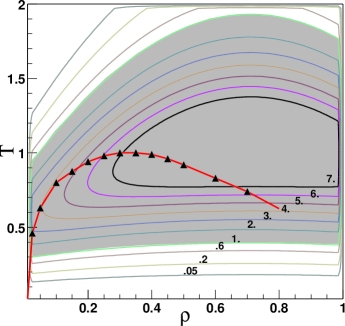
Figure 1: Phase diagram of a Lennard-Jones fluid with $N=64$ particles confined in a container. Iso-contour lines indicate values of the quantity $\sigma_{K^{\prime}}^{2}/T^{2}C_{1}$. When this quantity exceeds one (grey area), $c_{v}^{\prime}$ (see text) is negative. The position of the liquid-gas coexistence line is sketched by filled triangles. Temperature $T$ and density $\rho$ are in units of the Lennard-Jones potential.

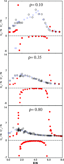
Figure 2: The heat capacity $c_{v}/N$ (open circles and open squares, see text) and the quantity $c_{v}^{\prime}/N$ (filled circles), as a function of the excitation energy per particle $E^{*}/N$ (in units $\epsilon$ of the Lennard-Jones potential) for isochore paths at $\rho=0.10,0.35$ and $0.80$.

We see that when $\sigma_{K^{\prime}}^{2}/T^{2}C_{1}>1$, $c^{\prime}_{v}$ becomes negative. Figure 1 reveals that this quantity exceeds one in a large zone of the density-temperature phase diagram. The location of the zone of maximal fluctuation of $K^{\prime}$ is easily understood. These fluctuations are nothing but those of the fragment mass distribution $n(A)$ and one expects these fluctuations to be maximum around the critical point. Indeed, if the binding energy of the fragments is well represented by a mass formula $B(A)=a_{v}A+a{s}A^{2/3}$, then $\sigma_{K^{\prime}}^{2}=a_{s}^{2}(<m_{2/3}^{2}>-<m_{2/3}>^{2})$, where $m_{2/3}$ is the standard moment of order $2/3$ of $n(A)$.

The above results show that, at least in the present model, $c^{\prime}_{v}$ is not a satisfactory representation of the heat capacity. Indeed, heat capacities cannot be negative in the (monophasic) super-critical region ($T>T_{critical}$). Moreover, molecular dynamics simulations indicate that in the present model $c_{v}$ is always positive (except in a small zone at very low density as in ref.[6] and at low temperatures around the liquid-solid transition as in ref. [2]). Examples of a comparison of $c_{v}$ and $c^{\prime}_{v}$ are given in Fig. 2 for isochore paths at $\rho=0.1$, $\rho=0.35$ and $\rho=0.80$. The heat capacities $c_{v}$ have been calculated from the fluctuations of $K$ (open circles) and from the derivatives of the caloric curve (open squares). One remarks that both agree very well. Note that for the density of $0.1$ and a narrow energy domain around $1.0$, the later method predicts a negative heat capacity.

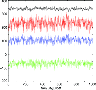
Figure 3: Time evolution of various quantities at a density of $\rho=0.35$ and excitation energy per particle of $E^{*}/N=4.12$. From top to bottom: $K$ (shifted by 250 units), $K^{\prime}$ (shifted by 100 units), $\sum_{i}(V_{i}-B_{i})$ and $\sum_{i<j}V_{i,j}$.

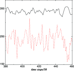
Figure 4: Time evolution of $K$ (continuous line) and $K^{\prime}$ (dashed line), with an enlarged time scale. Same conditions as for Fig.3

The origin of the discrepancy with the conclusions of Ref.[7, 8] can be localized by looking at the various components of K (equ.(2)) (see Fig.3 and 4). One immediately remarks that the fluctuation of $K^{\prime}$ largely exceeds the fluctuation of $K$. A closer examination (see Fig.4) also reveals that these fluctuations are not in phase. These discrepancies appear because the contributions of the terms $\sum_{i}(V_{i}-B_{i})$ and $\sum_{i<j}V_{i,j}$ have been neglected. We have observed that the contribution of the inter-fragment potential energy decreases with density but surprisingly, the fluctuation of the intra-fragment potential energy remains very important at all densities. This means that in the regions of density and temperature we are looking at, fragments are not compact spheres. From the above considerations it emerges that for the present simple model, where physics is well under control, $c_{v}^{\prime}$ is not a satisfactory approximation of the heat capacity.

The question that now naturally arises is to what extent this remains true for real nuclei. One of the main differences is the absence of Coulomb energy in our analysis. The motivation of our choice is that simpler is the model, clearer is the identification of the sources of discrepancy. We do not believe that including Coulomb interaction the situation would drastically change. Ison and Dorso [17] have shown that adding a Coulomb term to a Lennard-Jones potential produces no qualitative changes in the heat capacities of small systems. In any case, the problem of the inter-fragment [18] and intra-fragment energies will persist. By the way, if Coulomb was so important in nuclei, this would mean that the fluctuations are linked more to instabilities in a Coulomb gas than to a liquid-gas phase transition and the whole interpretation should be revised. Furthermore, one has to keep in mind that in the analysis of experimental data [7, 8] only part of the Coulomb fluctuations are extracted from experiment, because at each event the spatial distribution of fragments inside the fragmentation volume is unknown.

The present results illustrate once more the difficulty to study the thermodynamics of “small systems” from data that are (almost) limited to fragment size distributions measured after their expansion at very late times. We hope that the results presented here will stimulate the search for new approaches of this problem.

We are indebted to Ph. Chomaz, F. Gulminelli and M. D’Agostino for fruitful discussions and for pointing out an error in the plotting of Figures 3 and 4 of a previous version of this paper. We would also like to thank D.H.E. Gross for stimulating discussions on negative heat capacities in small systems.

References

- [1] D. H. E. Gross, Microcanonical Thermodynamics, Phase Transitions in “Small” Systems, World Scientific Lecture Notes in Physics, Vol. 66, World Scientific (2001); D.H.E. Gross, Chaos, Solitons and Fractals 13, 417 (2002).
- [2] P. Labastie and R. L. Whetten, Phys. Rev. Lett. 65, 1567 (1990).
- [3] Ph.Chomaz and F. Gulminelli, Nucl. Phys. A647, 153 (1999); Ph. Chomaz, V. Duflot and F. Gulminelli, Phys. Rev. Lett. 85, 3587 (2000).
- [4] F. Gulminelli, ’Phase Coexistence in Nuclei’, to be published.
- [5] M. Pleimling and A. Hueller, Jour. Stat. Phys. 104, 971 (2001).
- [6] A. Chernomoretz, M. Ison, S. Ortiz and C.O. Dorso, Phys. Rev. C64, 024606 (2001); M. J. Ison, A. Chernomoretz and C.O. Dorso, Physica A (2004), in press.
- [7] M. D’Agostino, F. Gulminelli, Ph. Chomaz, M. Bruno, F. Cannata, R. Bougault, F. Gramegna, I. Iori, N. Le Neindre, G. V. Margagliotti, A. Moroni, G. Vannini, Phys. Lett B473, 219 (2000).
- [8] M. D’Agostino, R. Bougault, F. Gulminelli, M. Bruno, F. Cannata, Ph. Chomaz, F. Gramegna, I. Iori, N. Le Neindre, G.V. Margagliotti, A. Moroni, G. Vannini, Nucl. Phys. A699, 795 (2002).
- [9] M. Schmidt, R. Kusche, T. Hipper, J. Donges, W.Kronmüller, B. von Issendorff and H. Haberland, Phys. Rev. Lett. 86, 1191 (2001).
- [10] F. Gobet, B. Farizon, M. Farizon, M.J. Gaillard, J.P. Buchet, M. Carré, P. Scheier and T.D. Märk, Phys. Rev. Lett. 89, 183403 (2002).
- [11] E. M.Pearson et al., Phys. Rev. A32, 3030 (1985).
- [12] W. Thirring, Z. Physik 235, 339 (1970).
- [13] X. Campi, H. Krivine, E. Plagnol and N. Sator, Phys. Rev. C67, 044610 (2003).
- [14] D.J. Wales and J.P.K. Doye, J. Phys. Chem. A101, 5111 (1997).
- [15] T.L. Hill, J. Chem. Phys. 23, 617 (1955).
- [16] C.O. Dorso and J. Randrup, Phys. Lett. B301, 328 (1993).
- [17] M.J. Ison and C.O. Dorso, Phys. Rev. C69, 027001 (2004).
- [18] S.K. Samadar, J.N. De and A. Bonasera, nucl-th 0402068.