Soft triaxial roto-vibrational motion in the vicinity of $\gamma=\pi/6$

Abstract

A solution of the Bohr collective hamiltonian for the $\beta-$soft, $\gamma-$soft triaxial rotor with $\gamma\sim\pi/6$ is presented making use of a harmonic potential in $\gamma$ and Coulomb-like and Kratzer-like potentials in $\beta$. It is shown that, while the $\gamma-$angular part in the present case gives rise to a straightforward extension of the rigid triaxial rotor energy in which an additive harmonic term appears, the inclusion of the $\beta$ part results instead in a non-trivial expression for the spectrum. The negative anharmonicities of the energy levels with respect to a simple rigid model are in qualitative agreement with general trends in the experimental data.

The search for new solutions of the Bohr collective hamiltonian has recently experienced a resurgence, mainly due to influential studies upon shape phase transitions Iac ; Iac2 . The occurrence of analytically solvable models has served to define benchmarks for the analysis of experimental nuclear spectra. As long as the quadrupole degree of freedom is considered, the nuclear Bohr-Mottelson collective model has a few well-known complete solutions that correspond to spherical or axially symmetric equilibrium intrinsic shapes. In some case, when the full solution is a demanding task, one has usually resorted to the so-called rigid models in which one or both of the deformation variables, $\beta$ and $\gamma$, is constrained to take a fixed value. The opposite situation, in which either the $\beta$ or $\gamma$ variable (or both) is not forced to take a fixed value, is called soft.

The purpose of the present paper is to present a novel solution of the Bohr collective hamiltonian for the $\beta-$soft, $\gamma-$soft triaxial rotor with $\gamma$ around $\pi/6$. Our model include $\beta$ and $\gamma$ vibrations as well as rotations about a non-axially symmetric equilibrium intrinsic shape.

Years ago Davydov Dav proposed a model for a rigid triaxial rotor, described diagonalizing the hamiltonian for a rigid rotor with three different moments of inertia. The corresponding soft cases, that are described by the full Bohr hamiltonian with some $V(\beta,\gamma)$ potential (that displays a pocket whose minimum lies in $\beta_{0}\neq 0,\gamma_{0}\neq 0$), has been only partially or numerically treated (see also Mey ). Davydov discussed also a model with soft behaviour with respect to $\beta$ DavCh and a model with soft behaviour with respect to $\gamma$ Dav2 . These approaches give rather complicated expressions for the spectrum. The latter, in which the effective potential in $\gamma$ is expanded in a series and truncated neglecting terms of order higher than the second, has some similarity with the present approach. Our model, although restricted to $\gamma\sim\pi/6$, is easier to handle and gives in a straightforward fashion the full energy spectrum, while the cited Davydov’s treatments give only the energies of a limited number of states.

This study is partly born out from the necessity to overcome the reservations on the above models (see for example Rowe ) about the neglected role of the fluctuations of the dynamic moments of inertia and partly to show that the naïve idea that the spectrum of a soft triaxial rotor will be the sum of a rigid rotor part plus a harmonic $\beta-$ and harmonic $\gamma-$vibrations is essentially incorrect. In the present case the solution of the $\gamma-$angular part is indeed a straightforward extension of the rigid triaxial rotor energy in which an additive harmonic term appears, but the inclusion of the $\beta$ part gives rise to a peculiar combination of the various terms.

A closely connected solution of the Bohr hamiltonian has recently appeared as a preprint Bon . The common point between this work and ours is the presence of a minimum in $\gamma=30^{o}$. In the cited work a critical point symmetry, called Z(5), is introduced for the prolate to oblate shape phase transition. The authors discuss the solution and compare their predictions with experimental data in the Pt region, obtaining a good agreement. The main difference between the two approaches lies essentially in the expressions of the potentials. Their potential may be written as $u_{1}(\beta)+u_{2}(\gamma)$, where a harmonic oscillator is used for the $\gamma$ variable, and where an infinite square well is used for the $\beta$ potential, similarly to what has been done in Refs. Iac ; Iac2 for the so-called E(5) and X(5) symmetries, thus achieving an approximate separation of variables. Anticipating the following discussion we mention that in the present solution a potential of the form (5) makes exact the separation of variables and Coulomb and Kratzer potentials are used in the $\beta$ variable.

Two very recent papers Jo1 deal with a similar subject: beside a detailed study on phase transition in nuclei in the framework of the interacting boson model, a summary of different solutions of the Bohr hamiltonian is done and an interesting solution for a triaxial case with $\gamma\sim\pi/6$ is discussed. The author assumes a potential of the form $V(\beta,\gamma)=u(\beta)+{1\over 2}D\beta^{6}\cos{3\gamma}$ and follows an approach similar to the one used in ref. Iac2 .

The Schrödinger equation with the Bohr hamiltonian may be written as

$$H_{B}\Psi(\beta,\gamma,\theta_{i})~{}=~{}E\Psi(\beta,\gamma,\theta_{i})$$ (1)

where $H_{B}~{}=~{}T_{\beta}+T_{\gamma}+T_{rot}+V(\beta,\gamma)$ Jean and the kinetic terms have the following expressions

$$T_{\beta} ~{}=~{}-\displaystyle{\hbar^{2}\over 2B_{m}}{1\over\beta^{4}}{\partial\over\partial\beta}\beta^{4}{\partial\over\partial\beta}$$ (2)

$$T_{\gamma} ~{}=~{}-\displaystyle{\hbar^{2}\over 2B_{m}}{1\over\beta^{2}}{1\over\sin{(3\gamma)}}{\partial\over\partial\gamma}\sin{(3\gamma)}{\partial\over\partial\gamma}$$ (3)

$$T_{rot} ~{}=~{}\displaystyle{\hbar^{2}\over 8B_{m}\beta^{2}}\sum_{\kappa=1,2,3}{{\hat{Q}}_{\kappa}^{2}\over\sin^{2}(\gamma-2\pi\kappa/3)}$$ (4)

where the ${\hat{Q}}_{\kappa}$ are the projections of the angular momentum ($\hat{L}$) in the intrinsic frame. The potential term is in general a function of $\beta$ and $\gamma$. The conditions, that must be imposed on this potential term in order to separate the above differential equation, have been discussed extensively in the literature (see for example Bohr ; WJ ; DavCh ). For our purposes it will be sufficient to notice that whenever the potential is chosen as

$$V(\beta,\gamma)~{}=~{}V_{1}(\beta)+{V_{2}(\gamma)\over\beta^{2}}\,,$$ (5)

the Schrödinger equation is separable WJ into the following set of second order differential equations:

$$\Bigl{(}T_{\beta}+V_{1}(\beta)-E+{\Omega\over\beta^{2}}\Bigr{)}f(\beta) ~{}=~{}0$$ (6)

$$\Bigl{(}\beta^{2}\bigl{(}T_{\gamma}+T_{rot}\bigr{)}+V_{2}(\gamma)-\Omega\Bigr{)}\Phi(\gamma,\theta_{i}) ~{}=~{}0$$ (7)

with $\Psi(\beta,\gamma,\theta_{i})~{}=~{}f(\beta)\Phi(\gamma,\theta_{i})$. Notice that the second equation does not depend on $\beta$. This separation of variables invokes a constant, $\Omega$. Here we solve the problem of a $\beta-$soft, $\gamma-$soft triaxial rotor with a potential that has a minimum located in $\beta=\beta_{0}$ and $\gamma=\gamma_{0}~{}=~{}\pi/6$. The simplest approach to this problem is to choose a displaced harmonic dependence for the $\gamma$ variable in order to have a pocket around the minimum. The potential in the asymmetry variable must be an even function of $\gamma$ because of the indistinguishability with respect to the change of sign of $\gamma$, and must also be a periodic function to assure that the operation of relabeling of the axes does not change the shape of the ellipsoid, but only its orientation. This statement is obviously not fulfilled by our choice that is to be considered therefore only locally in the region around the minimum. We notice that a discrete rotation of $n\pi/3$ in the polar coordinate system $(\beta,\gamma)$ does not affect our conclusions.

In the $\gamma-$rigid case with a situation of maximum asymmetry ( for $\gamma_{0}~{}=~{}\pi/6$) two of the moments of inertia are ’accidentally’ equal Brink ; priv , while the axes of the ellipsoid have not equal length. The hamiltonian is thus axially symmetric around the intrinsic 1-axis, that may be taken as a quantization axis, as pointed out in ref. Mey . We will restrict to a small region around $\pi/6$ to take advantage of this simplification. Before discussing how to solve the $\gamma-$soft case, we multiply the two equations above by $2B_{m}/\hbar^{2}$ and we define reduced energy and potentials as $\varepsilon~{}=~{}2B_{m}E/\hbar^{2}$ and $u_{i}(z)~{}=~{}2B_{m}V_{i}(z)/\hbar^{2}$ with $(i=1,2)$. Lower case symbols denote reduced quantities and operators. The new set of ’reduced’ equations, given the definitions $t_{i}=(2B_{m}/\hbar^{2})\beta^{2}\,T_{i}$ ($i={\gamma,rot}$) and $\omega~{}=~{}2B_{m}\Omega/\hbar^{2}$, is

$$\Bigl{(}-\displaystyle{1\over\beta^{4}}{\partial\over\partial\beta}\beta^{4}{\partial\over\partial\beta}+u_{1}(\beta)-\varepsilon+{\omega\over\beta^{2}}\Bigr{)}f(\beta)~{}=~{}0$$ (8)

$$\Bigl{(}t_{\gamma}+t_{rot}+u_{2}(\gamma)-\omega\Bigr{)}\Phi(\gamma,\theta_{i})~{}=~{}0$$ (9)

The spectrum is determined by the solution of the first differential equation in which $\omega$, that it is found from the solution of the second differential equation, plays the role of the coefficient of a ’centrifugal’ term and, as we will show, yields a non-trivial expression for the energy levels.

Around $\pi/6$ we may set $\gamma~{}=~{}\pi/6+x$, with $x$ a small expansion parameter. It is easily seen that in this case the rotational part of the Bohr hamiltonian, through use of trigonometric relations, becomes

$$\sum_{\kappa=1,2,3}{{\hat{Q}}_{\kappa}^{2}\over\sin^{2}(\gamma-2\pi\kappa/3)}~{}=~{}$$

$$~{}=~{}4(\underbrace{{\hat{Q}}_{1}^{2}+{\hat{Q}}_{2}^{2}+{\hat{Q}}_{3}^{2})}_{\displaystyle{\hat{L}}^{2}}+{\hat{Q}}_{1}^{2}\Biggl{(}{1\over\cos^{2}(x)}-4\Biggr{)}$$ (10)

where we have added and subtracted $4{\hat{Q}}_{1}^{2}$.

The first step to solve the $(\gamma,\theta_{i})$ part of the problem is to change variable in Eq. (9), using $\gamma=\pi/6+x$ and introducing the following simplifications:

$$\sin{3\gamma}=\cos{3x}\sim 1\qquad\,\,\cos{x}\sim 1.$$

We obtain, specifying the harmonic dependence of the potential, $u_{2}(x)~{}=~{}Cx^{2}$, and exploiting relation (10), the following equation

$$\Biggl{(}\underbrace{-{\partial^{2}\over\partial x^{2}}+Cx^{2}-\omega}_{\displaystyle\hat{H}_{1}}+{\hat{\vec{Q}}}^{2}-{3\over 4}{\hat{Q}_{1}}^{2}\Biggr{)}\Phi(x,\theta_{i})~{}=~{}0$$ (11)

where the second order differential operator $\hat{H}_{1}$ has been defined. The wavefunction $\Phi(x,\theta_{i})$ may be written, following Mey , as

$$\sqrt{2L+1\over 16\pi^{2}(1+\delta_{R,0})}\eta_{n_{\gamma},L,R}(x)\bigl{[}{\cal D}^{(L)}_{M,R}(\theta_{i})+(-1)^{L}{\cal D}^{(L)}_{M,-R}(\theta_{i})\bigr{]}$$ (12)

where the angular part is written in terms of Wigner functions labeled by the projection of the total angular momentum on the 1-axis, $R$, that is a good quantum number, while the functions $\eta_{n_{\gamma},L,R}(x)$ are eigenfunctions of the one dimensional Schrödinger equation for the harmonic oscillator, ${\hat{H}_{1}}\eta_{n_{\gamma},L,R}(x)=0$. The index $n_{\gamma}$ is the quantum number associated with the vibrations in the $\gamma$ degree of freedom. The action of the operators in eq. (11) on the respective wavefunctions gives

$$\omega_{L,R,n_{\gamma}}=\sqrt{C}(2n_{\gamma}+1)+L(L+1)-{3\over 4}R^{2}$$ (13)

The first term corresponds to a harmonic $\gamma-$vibration, while the second and third account for the rotational energy of the $\gamma=\pi/6$ rigid triaxial rotor, reproducing the Meyer-ter-vehn formula Mey .

The complete spectrum may then be obtained solving eq. (8) with some appropriate potential, $u_{1}(\beta)$, as, for instance, in Ref. Iac ; Iac2 ; Bohr ; WJ ; RoBa ; FV ; Elli ; FV2 . The eigenvalue equation in the $\beta$ variable may in general be written as

$$\chi^{\prime\prime}(\beta)+\Bigl{(}\varepsilon-u_{1}(\beta)-{\omega+2\over\beta^{2}}\Bigr{)}\chi(\beta)=0$$ (14)

having imposed $f(\beta)~{}=~{}\beta^{-2}\chi(\beta)$. When the potential $u_{1}(\beta)$ is taken to be of a FV ; FV2 Coulomb-like form $-A/\beta$, or of a Kratzer-like form $-A/\beta+B/\beta^{2}$, with the substitutions $z=2\beta\sqrt{\epsilon}$, $\epsilon=-\varepsilon$, $k=A/(2\sqrt{\epsilon})$ and $\mu^{2}=9/4+B+\omega$, we can recast equation (14) as the Whittaker’s differential equation:

$$\Bigl{\{}{d^{2}\over dz^{2}}-{1\over 4}+{k\over z}+{1/4-\mu^{2}\over z^{2}}\Bigr{\}}\chi(z)=0$$ (15)

whose well-known solution is expressed in terms of Whittaker’s functions. As in FV ; FV2 the requirement of the correct asymptotic behaviour fixes the spectrum, introducing the $n_{\beta}$ quantum number associated with $\beta-$vibrations. The reduced eigenvalues are

$$\epsilon(n_{\gamma},n_{\beta},L,R)={A^{2}/4\over\Bigl{(}\sqrt{9/4+B+\omega_{L,R,n_{\gamma}}}+1/2+n_{\beta}\Bigr{)}^{2}}$$ (16)

where $\omega$ comes from eq. (13). Energies are usually redefined fixing the ground state to zero and using the energy of the first $2^{+}$ state as unit, namely

$$\bar{\epsilon}(n_{\gamma},n_{\beta},L,R)={\epsilon(n_{\gamma},n_{\beta},L,R)-\epsilon(0,0,0,0)\over\epsilon(0,0,2,2)-\epsilon(0,0,0,0)}~{}~{}.$$ (17)

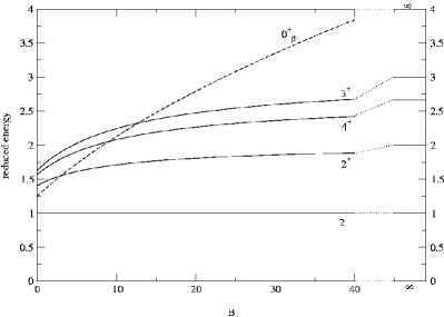
Figure 1: Reduced energies of the lowest state of the $\beta-$band (dashed line) and of a few lowest states of the ground state band (solid lines) as a function of $B$. The limits for the energy levels when $B\rightarrow\infty$, that correspond to the rigid triaxial rotor energies, are reported in the right side. Here we fixed $C=1$.

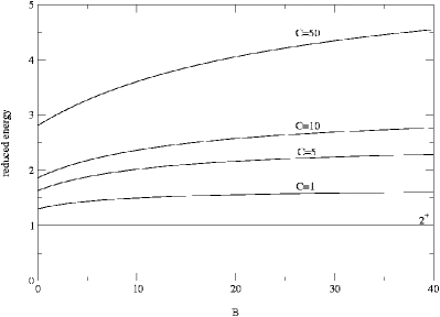
Figure 2: Reduced energies of the ($J^{\pi}=2^{+},n_{\gamma}=1,n_{\beta}=0$) state (solid line) as a function of $B$, for various values of the strength of the harmonic potential in $\gamma$, $C$. The first $2^{+}$ of the ground state band (dashed line) is reported for reference.

In fig. (1) we displayed, as a function of $B$ and for a fixed value of $C=1$, the lowest states of the ground state band ($n_{\beta}=0,n_{\gamma}=0$) and the lowest $0^{+}$ of the $\beta-$band ($n_{\beta}=1,n_{\gamma}=0$). It may be seen that when $B\rightarrow\infty$ the typical rigid rotor energies are recovered from the limit of the ground state energy levels. The relative position of the $\beta-$band (eventually tending to infinity), with respect to the ground state band, gives an idea of the degree of $\beta-$softness. The negative anharmonicities evidenced in this figure (that are strictly valid for a triaxial nucleus with $\gamma\sim 30^{o}$) are qualitatively consistent with most experimental data on triaxial nuclei where typically the $3^{+}$ and $4^{+}$ states are found at an energy that is lower than the rigid rotor prediction. In fig. (2) we plotted the lowest $2^{+}$ state of the ground state band for reference and the $(J^{\pi}=2^{+},n_{\gamma}=1,n_{\beta}=0)$ state for various values of the parameter $C$, that is the strength of the harmonic oscillator in $\gamma$. A low value for $C$ corresponds to a soft well, while a large value corresponds to a more rigid situation. When $B\rightarrow\infty$ the states of the $\gamma-$band tend to finite values, as far as $C$ is finite. The Wilets-Jean limit (complying with the choice of Coulomb and Kratzer potentials in $\beta$ FV ) is correctly obtained from formula (16) when the $\gamma-$potential becomes flat ($C=0$). The reduced energy spectra shown in both figures do not depend on the parameter $A$. This model has, from one side, a limited applicability because it is confined to some special triaxial nuclei for which the minimum of the potential lies at $\gamma=\pi/6$, but from the other side, it has a considerable flexibility as far as the position of the excited bands is concerned. The interplay between the two parameters may be exploited to fit experimental data. Notice that $B$ and $C$ do not separately fix the position of the respective $\beta$ and $\gamma$ bands, but they both take part in a non-trivial way to determine the energy levels. It is nevertheless very well known Cast that many predictions obtained for a $\gamma-$rigid model nearly agree with an axially symmetric $\gamma-$soft model whenever the $\gamma_{rms}$ of the latter equals the rigid value of the former. This fact may increase the applicability of the model.

The addition of $\gamma$ and $\beta$ vibrations to the rigid triaxial rotor spectrum (around $\gamma=30^{o}$) shows interesting features: the well-accepted naïve idea that the spectrum of the soft rotor is approximatively the sum of a rigid rotor term plus separate vibrational terms in $\beta$ and in $\gamma$ is not necessarily correct. Indeed we have shown that, while the solution of the $\gamma-$angular part of the problem gives a straightforward extension of the rigid rotor formula in which a simple harmonic term for the $\gamma$ degree of freedom appears, the full spectrum is rather a more complicated function that essentially depends on the choice of the potential in $\beta$. Other choices are possible as, for instance, a displaced harmonic oscillator or a Davidson potential RoBa ; Elli in $\beta$, that lead to exact solutions. The solution presented here may well serve as a good starting point to analyze energy spectra in various mass regions where triaxiality is expected to play a relevant role.

I wish to thank F.Iachello for having called my attention to this problem, I.Hamamoto, M.A.Caprio, K.Heyde and A.Vitturi for valuable discussions and D.J.Rowe for enlightening comments. I acknowledge financial support from FWO-Vlaanderen and from Università di Padova, where this work was started.

References

- (1) F.Iachello, Phys.Rev.Lett. 85, 3580 (2000).
- (2) F.Iachello, Phys.Rev.Lett. 87, 052502 (2001).
- (3) A.S.Davydov and G.F.Filippov, Nucl.Phys. 8, 237 (1958); A.S.Davydov and V.S.Rovstovsky, Nucl.Phys. 12, 58 (1959).
- (4) J.Meyer-ter-vehn, Nucl.Phys. A249, 111 (1975).
- (5) A.S.Davydov and A.A.Chaban, Nucl.Phys. 20, 499-508 (1960).
- (6) A.S.Davydov, Nucl.Phys. 24, 682 (1961).
- (7) D.J.Rowe, Nuclear Collective motion (1970) Methuen and Co. LTD., London.
- (8) D.Bonatsos et al., Phys.Lett. 588, 172 (2004).
-
(9)
R.V.Jolos, Phys.Atom.Nucl. 67, 931 (2004);
ibid., Phys.Part.Nucl. 35, 225 (2004). - (10) M.Jean, Nucl. Phys. 21, 142 (1960).
- (11) A.Bohr, Dan.Mat.Fys.Medd. 26 (1952) vol. 14.
- (12) L.Wilets and M.Jean, Phys. Rev. 102, 788 (1956).
- (13) D.M.Brink, Prog.Nucl.Phys.8, 97 (1960).
- (14) F.Iachello, private communication.
- (15) D.J.Rowe and C.Bahri, J.Phys.A: Math.Gen 31, 4947 (1998).
- (16) L.Fortunato and A.Vitturi, J.Phys.G: Nucl.Part.Phys 29, 1341 (2003).
- (17) J.P.Elliott et al., Phys.Lett. 169B, 309 (1986).
- (18) L.Fortunato and A.Vitturi, J.Phys.G: Nucl.Part.Phys 30, 627-635 (2004).
- (19) R.F.Casten, Nuclear Structure from a simple perspective, 2nd Ed. (2000) Oxford Un. Press Inc., New York.