Damped collective motion of isolated many body systems within a variational approach to functional integrals

Abstract

Two improvements with respect to previous formulations are presented for the calculation of the partition function $\mathcal{Z}$ of small, isolated and interacting many body systems. By including anharmonicities and employing a variational approach quantum effects can be treated even at very low temperatures. A method is proposed of how to include collisional damping. Finally, our approach is applied to the calculation of the decay rate of metastable systems.

Small many body systems like atomic nuclei and metal clusters may undergo self-sustained collective motion. In the former case this has long been established experimentally for situations where the nucleons may be assumed to move in a time-dependent state with no additional excitation energy bm . In the last few years one is also able to measure properties of single, isolated metallic grains grains . Although such systems consist of (many) particles of identical or similar nature collective motion only involves one or a few time dependent parameters. The latter must be introduced so that they obey certain basic relations for the intrinsic (particle) degrees of freedom. One, formally promising way is to apply the functional integral technique and to introduce collective degrees of freedom via a Hubbard-Stratonovich transform (HST). This is especially useful when the nature of the collective motion can be guessed and attributed to one generator $\hat{F}$. Following bm one may then introduce a separable two-body interaction to obtain for the total Hamiltonian

$$\hat{H}=\hat{H}_{0}+\frac{k}{2}\,\hat{F}\hat{F}\,,$$ (1)

in which the coupling constant $k$ is negative for iso-scalar modes. Of course, this might be understood as one prominent term in an expansion of a general two-body interaction $\hat{V}^{(2)}$ into a complete series of separable terms like $\hat{H}=\hat{T}+\hat{V}^{(2)}=\hat{H}_{0}+\frac{1}{2}\sum_{\mu=1}^{m}k_{\mu}\,\hat{F}^{\mu}\hat{F}^{\mu}$. For the sake of simplicity we will restrict our discussion to the model case (1), but treatments of more terms are feasible and have already been undertaken for applications which are simpler than those we have in mind (see e.g. ath.aly:npa:97 ). For zero thermal excitation the $\hat{H}_{0}$ might be assumed to simply represent the dynamics of independent particles. However, in case the constituents themselves are excited this may no longer be true as then incoherent, residual interactions $\hat{V}_{\textrm{res}}^{(2)}$ may play a role, with an ever increasing role the larger the excitation. In the nuclear case it is known that single particle excitations acquire a finite width if they are away from the Fermi level by only $5-8$ MeV mahauxsartor:91 . This effect is further enhanced if the system of particles is thermally excited. In the present Letter we want to show how these effects may be accounted for in the functional integral approach. Moreover, in contrast to previous formulations ath.aly:npa:97 ; SPA ; PSPA , we also demonstrate the usefulness of generalizing the variational formulation of var-ital ; fer.klh:pra:86 to many body systems. In this way one may overcome the divergence known to exist for small temperatures in the case where the collective motion passes over barrier regions.

Our basic theoretical tool will be the partition function $\mathcal{Z}$ which at given temperature $T=1/(k_{\textrm{B}}\beta)$ may be expressed as ath.aly:npa:97

$$\mathcal{Z}(\beta)=\sqrt{\frac{\beta}{2\pi|k|}}\int dq_{0}\ \exp[-\beta\mathcal{F}^{\textrm{SPA}}(\beta,q_{0})]\ \zeta(\beta,q_{0})\,.$$ (2)

The $\mathcal{F}^{\textrm{SPA}}(\beta,q_{0})$ is a free energy which depends on the collective variable $q_{0}$, treated here in the static limit, which in this context in the literature is referred to as “Static Path Approximation” (SPA) SPA . It may be written as $\mathcal{F}^{\textrm{SPA}}(\beta,q_{0})=q_{0}^{2}/(2|k|)-T\,\textrm{ln}\,z(\beta,q_{0})$, where $z(\beta,q_{0})$ is the grand canonical partition function calculated for the static one body hamiltonian $\hat{\mathcal{H}}_{\textrm{HST}}[q_{0}]=\hat{H}_{0}+q_{0}\hat{F}$. Actually, the collective variable is ”time-dependent” and is introduced via the HST. Using this manipulation the two body interaction $k\hat{F}\hat{F}/2$ disappears. The dependence on the imaginary time $\tau$ is treated through the Fourier series $q(\tau)=q_{0}+\sum_{r\neq 0}q_{r}\,\exp(\textrm{i}\nu_{r}\tau)$, with the Matsubara frequencies $\nu_{r}=2\pi r/(\hbar\beta)=2\pi rT/\hbar$. Genuine quantum effects in collective motion are hidden in the factor

$$\zeta(\beta,q_{0})=\int\mathcal{D}^{\prime}q\ \exp[-s_{\textrm{E}}(\beta,q_{0})/\hbar]\,.$$ (3)

The key stone for improvements over the SPA is given by the Euclidean action $s_{\textrm{E}}$. In the so called “Perturbed SPA” (PSPA) – also known as “SPA+RPA” or “Correlated SPA” (CSPA) – this $s_{\textrm{E}}$ is expanded to second order in the $q_{r}$. In this way quantum effects are treated at the level of a local RPA, see e.g. PSPA ; ath.aly:npa:97 ; ruc.hoh:pre:01 . In an extension of this approximation we shall want to make use of terms up to fourth order and write the action as (see also rummel:phd ; ruc.anj:epjb:02 )

$$s_{\textrm{E}}(\beta,q_{0})=\frac{\hbar\beta}{|k|}\left(\sum_{r,s\neq 0}\lambda_{rs}\,q_{r}q_{s}+\sum_{r,s,t\neq 0}\rho_{rst}\,q_{r}q_{s}q_{t}+\sum_{r,s,t,u\neq 0}\sigma_{rstu}\,q_{r}q_{s}q_{t}q_{u}\right)+\mathcal{O}(q_{r}^{5})$$ (4)

The interesting point is that the coefficients $\lambda$, $\rho$ and $\sigma$ can be expressed by the one body Green functions associated with the Hamiltonian $\hat{\mathcal{H}}_{\textrm{HST}}[q_{0}]$, which at first may be assumed to represent simply independent particles for which the Green function is $g_{k}^{(0)}(z)=(z-\epsilon_{k})^{-1}$. In such a case the coefficient $\sigma_{rstu}$ of fourth order consists of terms like ruc.anj:epjb:02 ; rummel:phd

$$\frac{|k|}{4!}\sum_{i,k,m,o}F_{io}F_{ki}F_{mk}F_{om}\times$$ (5)

$$\left\{n(\epsilon_{i})\ g_{o}^{(0)}(\omega_{i}+\textrm{i}\nu_{r})\ g_{k}^{(0)}(\omega_{i}-\textrm{i}\nu_{s})\ g_{m}^{(0)}(\omega_{i}-\textrm{i}\nu_{s+t})+\ n(\epsilon_{o})\ g_{i}^{(0)}(\omega_{o}-\textrm{i}\nu_{r})\ g_{k}^{(0)}(\omega_{o}-\textrm{i}\nu_{r+s})\ g_{m}^{(0)}(\omega_{o}-\textrm{i}\nu_{r+s+t})\right.$$

$$\left.+\ n(\epsilon_{k})\ g_{i}^{(0)}(\omega_{k}+\textrm{i}\nu_{s})\ g_{o}^{(0)}(\omega_{k}+\textrm{i}\nu_{r+s})\ g_{m}^{(0)}(\omega_{k}-\textrm{i}\nu_{t})+\ n(\epsilon_{m})\ g_{i}^{(0)}(\omega_{m}+\textrm{i}\nu_{s+t})\ g_{o}^{(0)}(\omega_{m}+\textrm{i}\nu_{r+s+t})\ g_{k}^{(0)}(\omega_{m}+\textrm{i}\nu_{t})\right\}$$

to give just one example of what these quantities look like.

At the level of PSPA it is useful to connect the coefficient $\lambda$ to the response function $\chi(\omega)$ defined through $\delta\langle\hat{F}\rangle_{\omega}=-\chi(\omega)\,\delta q(\omega)$. One gets ruc.hoh:pre:01

$$\lambda_{rs}=\frac{1}{2}\,(1+k\chi(\textrm{i}\nu_{r}))\,\delta_{r,-s}=\frac{1}{2}\,\lambda_{r}\,\delta_{r,-s}\,.$$ (6)

The $\lambda_{r}$ serves as the stiffness in $q_{r}$-direction:

$$s_{\textrm{E}}^{\textrm{PSPA}}=\frac{\hbar\beta}{|k|}\sum_{r>0}\lambda_{r}\,|q_{r}|^{2}=\frac{\hbar\beta}{|k|}\sum_{r>0}\frac{\prod_{\mu}(\nu_{r}^{2}+\varpi_{\mu}^{2})}{\prod_{k>l}^{\prime}(\nu_{r}^{2}+\omega_{kl}^{2})}\,|q_{r}|^{2}$$ (7)

The unperturbed intrinsic excitations $\hbar\omega_{kl}=\epsilon_{k}-\epsilon_{l}$ are to be calculated from the eigenvalues of $\hat{\mathcal{H}}_{\textrm{HST}}[q_{0}]$. The $\varpi_{\mu}$, on the other hand, are to be found from the secular equation $1+k\,\chi(\varpi_{\mu})=0$ and represent the local RPA frequencies. For an unstable collective mode $\mu$ the $\varpi_{\mu}^{2}$ is negative such that $\lambda_{1}$ may become negative as well. This happens for temperatures below the so called crossover temperature $T_{0}$. There the dynamical fluctuations in $q_{1}$-direction become too large for the harmonic approximation to be justified. Formally, this shows up when in (3) Gaussian integrals become divergent ruc.hoh:pre:01 ; ruc.anj:epjb:02 ; rummel:phd . The name crossover temperature is borrowed from work on ”dissipative tunneling” within the Caldeira-Leggett model (CLM), where a similar breakdown is observed, see e.g. weissu . From this work it is known that in the crossover region $T\approx T_{0}$ the situation can be cured by treating the anharmonicities in $q_{1}$-direction explicitly up to fourth order. In this way it is possible to remove the divergence of the decay rate at $T_{0}$ in the CLM grh.olp.weu:prb:87 . In ruc.anj:epjb:02 this technique has been applied to many body systems to overcome the shortcomings of the PSPA. Using this “Extended PSPA” (ePSPA) the partition function can be evaluated down to $T=T_{0}/2$ where the fluctuations in $q_{2}$-direction become large, too. At very low temperatures the harmonic treatment of the fluctuations is no longer justified in any direction $q_{r}$. This feature prevents analytic treatments of higher modes $q_{r}$.

Such problems may largely be abolished by applying a variational procedure. In var-ital ; fer.klh:pra:86 the latter has been developed for the system of a particle moving in a one dimensional potential. It allows one to evaluate the quantum $\mathcal{Z}$ at arbitrary temperatures. Using the formalism of coherent states, these ideas have been applied to many body systems in yos.kic.nak.noh:prc:00 . Here we want to make use of the expansion (4). Details of this novel method will be given in a forthcoming paper. The main idea consists in rewriting (3) as

$$\zeta(\beta,q_{0}) = \int{\cal D}^{\prime}q\ \exp[-s_{\Omega}^{q_{0}}/\hbar]\ \exp[-(s_{\textrm{E}}-s_{\Omega}^{q_{0}})/\hbar]$$ (8)

$$= \zeta_{\Omega}^{q_{0}}\left\langle\exp[-(s_{\textrm{E}}-s_{\Omega}^{q_{0}})/\hbar]\right\rangle_{\Omega}^{q_{0}}\,.$$

The reference action $s_{\Omega}^{q_{0}}$ is introduced to specify an averaging procedure for which one may exploit the inequality

$$\left\langle\exp[-(s_{\textrm{E}}-s_{\Omega}^{q_{0}})/\hbar]\right\rangle_{\Omega}^{q_{0}}\geq\exp[-\langle s_{\textrm{E}}-s_{\Omega}^{q_{0}}\rangle_{\Omega}^{q_{0}}/\hbar]$$ (9)

for an optimization of the expression on the right hand side, which is easier to evaluate than the average in (8). The reference action should be chosen such that the normalization factor $\zeta_{\Omega}^{q_{0}}=\int{\cal D}^{\prime}q\ \exp[-s_{\Omega}^{q_{0}}/\hbar]$ in (8) can be evaluated exactly. A reasonable choice can be constructed from the PSPA action (7) by replacing the RPA frequencies $\varpi_{\mu}$ by variational parameters $\Omega_{\mu}$ rummel:phd :

$$s_{\Omega}^{q_{0}}=\frac{\hbar\beta}{|k|}\sum_{r>0}\frac{\prod_{\mu}(\nu_{r}^{2}+\Omega_{\mu}^{2})}{\prod_{k>l}^{\prime}(\nu_{r}^{2}+\omega_{kl}^{2})}\,|q_{r}|^{2}$$ (10)

Evidently, when calculating the integrals for $\langle s_{\textrm{E}}-s_{\Omega}^{q_{0}}\rangle_{\Omega}^{q_{0}}$ all terms disappear which are odd in $q_{r}$. Hence, in the truncated expansion (4) only terms of second and fourth order survive. Using the abbreviation $\Pi_{r}=\prod_{\mu}(\nu_{r}^{2}+\varpi_{\mu}^{2})-\prod_{\mu}(\nu_{r}^{2}+\Omega_{\mu}^{2})$ they can be written as:

$$\langle s_{\textrm{E}}^{\textrm{PSPA}}-s_{\Omega}^{q_{0}}\rangle_{\Omega}^{q_{0}} = \hbar\sum_{r>0}\frac{\Pi_{r}}{\prod_{\mu}(\nu_{r}^{2}+\Omega_{\mu}^{2})}$$ (11)

$$\langle\delta s_{\textrm{E}}^{(4)}\rangle_{\Omega}^{q_{0}} = \frac{\hbar|k|}{\beta}\sum_{r,s>0}\sigma_{rs-r-s}\,\frac{\prod_{k>l}^{\prime}(\nu_{r}^{2}+\omega_{kl}^{2})}{\prod_{\mu}(\nu_{r}^{2}+\Omega_{\mu}^{2})}\,\frac{\prod_{k>l}^{\prime}(\nu_{s}^{2}+\omega_{kl}^{2})}{\prod_{\mu}(\nu_{s}^{2}+\Omega_{\mu}^{2})}\ .$$ (12)

Collecting all contributions the dynamical corrections read

$$\textrm{ln}\,\zeta^{\textrm{var}}=\textrm{ln}\,\zeta_{\Omega}^{q_{0}}-\frac{1}{\hbar}\langle s_{\textrm{E}}^{\textrm{PSPA}}-s_{\Omega}^{q_{0}}\rangle_{\Omega}^{q_{0}}-\frac{1}{\hbar}\langle\delta s_{\textrm{E}}^{(4)}\rangle_{\Omega}^{q_{0}}\,,$$ (13)

which cannot be larger than $\textrm{ln}\zeta$. The advantage of this novel method over the PSPA and the ePSPA is that it can be applied at any $T$. The reason is that in contrast to the case of the PSPA the factors $\nu_{r}^{2}+\Omega_{\mu}^{2}$, which contribute to the stiffness in $q_{r}$-direction in (10), stay positive for all $\Omega_{\mu}$. Consequently all Gaussian integrals in (13) converge.

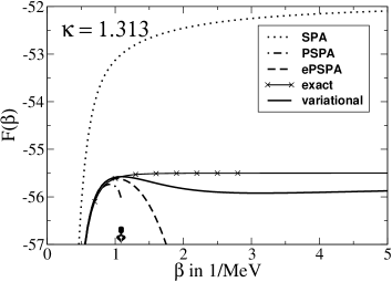
Figure 1: Free energy of the many body system for the LMGM with effective coupling constant $\kappa=1.313$ in various approximations. The arrow points to the inverse cross-over temperature $\beta_{0}=1/T_{0}$ where the PSPA breaks down.

To test the results we apply the exactly solvable Lipkin-Meshkov-Glick model (LMGM) lih.men.gla:np:65 , as used before in ath.aly:npa:97 ; PSPA for the the SPA and the PSPA. In Fig. 1 the free energy $\mathcal{F}=-T\ \textrm{ln}\,\mathcal{Z}$ associated to the total Hamiltonian (1) is compared with the approximations mentioned before. For the calculation the same set of parameters has been taken as in ruc.anj:epjb:02 . The classical SPA gives reasonable results only at small $\beta$ (high $T$). Inclusion of quantum effects at the level of local RPA within the PSPA delivers considerable improvement at not too large $\beta$. However, even before its breakdown at $\beta=\beta_{0}$ it becomes unreliable. The ePSPA behaves completely smoothly in the crossover region but breaks down at $\beta=2\beta_{0}$. Compared to these results, the improvement found for the variational approach is very striking. Notice please that it is free of discontinuities and the relative error is only of the order of 1%, even at very large $\beta$.

So far the one body Green’s functions $g_{k}^{(0)}(z)$ have been calculated within the picture of independent particle motion. As mentioned before, within this model the residual two body interaction $\hat{V}_{\textrm{res}}^{(2)}$ is neglected. This interaction describes the incoherent scattering of particles and holes and couples $1$p$1$h states to more complicated ones. This mechanism may be understood as the origin of the damping of collective motion, see e.g. hoh:pr:97 . In the following we will account for such couplings by dressing the one body Green functions with self-energies $\Sigma=\Sigma^{\prime}-\textrm{i}\Gamma/2$ meaning that $g_{k}^{(0)}(z)$ is replaced by

$$g_{k}^{(\Gamma)}(z)=\left(z-\epsilon_{k}-\Sigma_{k}^{\prime}(z)+\textrm{i}\Gamma_{k}(z)/2\right)^{-1}$$ (14)

The dependence of the width $\Gamma_{k}(\omega)$ on frequency and its variation with temperature is parameterized by the form

$$\Gamma_{k}(\omega)=\frac{1}{\Gamma_{0}}\,\frac{(\hbar\omega-\mu)^{2}+\pi^{2}T^{2}}{1+\frac{1}{c^{2}}[(\hbar\omega-\mu)^{2}+\pi^{2}T^{2}]}$$ (15)

suggested in siemensetal:84 . For zero temperature it is in good agreement with empirical data for the widths of proton and neutron states mahauxsartor:91 . Finally, some comments are in order concerning our approximation in handling the impact of $\hat{V}_{\textrm{res}}^{(2)}$. What is definitely implied in evaluating many-body Green functions is the application of a factorization assumption. However, it should be noticed that this is done for excitations of the intrinsic dynamics and not for the collective modes. One may therefore argue that coherent effects are small, in particular at larger thermal excitations. After all the SPA is meant to represent the high temperature limit.

Having established the connection between the PSPA and the theory of linear response one may take over the method developed there (see hoh:pr:97 ) to extract transport coefficients for collective dynamics. For slow collective motion, as given for nuclear fission, it suffices to concentrate on the lowest mode of the collective response function. In that frequency regime, the latter may then be approximated by the response function of a damped harmonic oscillator, which means the replacement:

$$\chi_{\textrm{coll}}(\omega)=\frac{\chi(\omega)}{1+k\chi(\omega)}\quad\longrightarrow\quad\chi_{\textrm{osc}}(\omega)$$ (16)

At any $q_{0}$ the $\chi_{\textrm{osc}}(\omega)$ is uniquely related to the coefficients of the local motion such as the inertia, friction and stiffness. It should be mentioned that exactly at this point an important difference to the CLM shows up. The latter only allows a microscopic interpretation of dissipation but not for the collective potential nor for the inertia. Conversely, our approach allows us to determine all coefficients in a self-consistent fashion, and all of them are influenced by the microscopic damping mechanism. It may be noted that the replacement of $g_{k}^{(0)}(z)$ by the $g_{k}^{(\Gamma)}(z)$ also influences the anharmonic terms of the Euclidean action, see (5). With respect to the variational approach the reduction (16) leads to a considerable simplification: Only one variational parameter $\Omega$ has to be dealt with in (10) to (13).

Let us finally turn to the decay rate of meta-stable states. As shown by J. S. Langer laj:ap:69 this rate can be related to the imaginary part of the free energy. Indeed, the CLM makes extensive use of this feature weissu . We will take this procedure over to the case of the interacting many body system. In order to obtain $\textrm{Im}\,\mathcal{F}$ from the $\mathcal{Z}$ in (2) the integration contour has to be deformed into the complex $q_{0}$-plane. This has to be done at the barrier of $\mathcal{F}^{\textrm{SPA}}$ in the sense of a steepest descent approximation. Details of the resulting rate formula for interacting many body problems will be given in a forthcoming paper. The quantum corrections $f_{\textrm{qm}}=\zeta_{b}/\zeta_{a}\geq 1$ to the purely classical rate formula of the SPA can be calculated from the dynamical factor $\zeta$ of (2) evaluated at the barrier $b$ and at the minimum $a$ of $\mathcal{F}^{\textrm{SPA}}$ within the approximations discussed above.

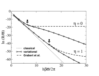
Figure 2: A comparison of different approaches to the decay rate for a particle in a one-dimensional cubic potential with barrier, for zero ($\eta=0$) and critical ($\eta=1$) damping. The arrows point to the $\beta_{0}=1/T_{0}$ where the PSPA breaks down.

To compare the various approaches to $\mathcal{Z}$ with respect to the evaluation of the quantum decay rate we take the case of a particle moving in a one dimensional cubic potential with barrier grh.olp.weu:prb:87 . For such a situation our variational approach reduces to the Feynman-Kleinert method (FKV) fer.klh:pra:86 . Results are shown in Fig. 2. The classical rate (SPA) just displays the exponential behavior of the Arrhenius law. Quantum corrections are known to increase the decay rate at larger $\beta$ (low $T$). The variational approach smoothly matches the classical result to the low $T$ result obtained by Grabert et al. with the dynamical “bounce solution” grh.olp.weu:prb:87 . In the region $\beta<\beta_{0}$ the PSPA would show a similar behavior with the exception of the crossover region itself. Different to the PSPA the variational approach gives good results also for $\beta\approx\beta_{0}$ but also fails in the regime $\beta\gg\beta_{0}$. This behavior may perhaps be understood as follows. Our variational approach in its present version starts from a static approximation and only includes small quantum corrections. For very large $\beta$ (low $T$) this cannot be enough as one ought to start from genuine time-dependent paths $q(\tau)$, like those associated to the “bounce solution” in the CLM. For the many body problem with dynamics beyond independent particle motion, however, this is still an open problem.

- (1) A. Bohr and B. Mottelson, Nuclear Structure (Benjamin, London, 1975).
- (2) D. Ralph et al., Phys. Rev. Lett. 74, 3241 (1995); ibid. 76, 688 (1996); ibid. 78, 4087 (1997).
- (3) H. Attias and Y. Alhassid, Nucl. Phys. A 625, 565 (1997).
- (4) C. Mahaux and R. Sartor, in Advances in nuclear physics, edited by J. Negele and E. Vogt (Plenum Press, New York, 1991), Vol. 20.
- (5) B. Mühlschlegel et al., Phys. Rev. B 6, 1767 (1972); Y. Alhassid and J. Zingman, Phys. Rev. C 30, 684 (1984); P. Arve et al., Ann. Phys. (N.Y.) 183, 309 (1988).
- (6) G. Puddu et al., Ann. Phys. (San Diego) 206, 409 (1991); R. Rossignoli and P. Ring, Nucl. Phys. A 633, 613 (1998).
- (7) R. Giachetti and V. Tognetti, Phys. Rev. Lett. 55, 912 (1985); R. Giachetti and V. Tognetti, Phys. Rev. B 33, 7647 (1986).
- (8) R. P. Feynman and H. Kleinert, Phys. Rev. A 34, 5080 (1986).
- (9) C. Rummel and H. Hofmann, Phys. Rev. E 64, 066126 (2001).
- (10) C. Rummel and J. Ankerhold, Eur. Phys. J. B 29, 105 (2002).
- (11) C. Rummel, Ph.D. thesis, Technische Universität München, 2004.
- (12) U. Weiss, Quantum Dissipative Systems (World Scientific, Singapore, 1993).
- (13) H. Grabert et al., Phys. Rev. B 36, 1931 (1987).
- (14) S. K. You et al., Phys. Rev. C 62, 045503 (2000).
- (15) H. J. Lipkin et al., Nucl. Phys. 62, 188 (1965).
- (16) H. Hofmann, Phys. Rep. 284 (4&5), 137 (1997).
- (17) P. Siemens et al., in Nucleon-Nucleon Interaction and the Nuclear Many-Body Problem, edited by S. Wu and T. Kuo (World Scientific, Singapore, 1984), p. 231.
- (18) J. S. Langer, Ann. Phys. (N.Y.) 54, 258 (1969).