Nuclear Structure based on Correlated Realistic Nucleon-Nucleon Potentials

Abstract

We present a novel scheme for nuclear structure calculations based on realistic nucleon-nucleon potentials. The essential ingredient is the explicit treatment of the dominant interaction-induced correlations by means of the Unitary Correlation Operator Method (UCOM). Short-range central and tensor correlations are imprinted into simple, uncorrelated many-body states through a state-independent unitary transformation. Applying the unitary transformation to the realistic Hamiltonian leads to a correlated, low-momentum interaction, well suited for all kinds of many-body models, e.g., Hartree-Fock or shell-model. We employ the correlated interaction, supplemented by a phenomenological correction to account for genuine three-body forces, in the framework of variational calculations with antisymmetrised Gaussian trial states (Fermionic Molecular Dynamics). Ground state properties of nuclei up to mass numbers $A\lesssim 60$ are discussed. Binding energies, charge radii, and charge distributions are in good agreement with experimental data. We perform angular momentum projections of the intrinsically deformed variational states to extract rotational spectra.

, , , and

1 Introduction

The advent of realistic nucleon-nucleon (NN) potentials has created a supreme challenge and opportunity for nuclear structure theory: the ab initio description of nuclei. Several families of realistic or modern NN potentials have been developed over the past three decades — among others the Argonne, Bonn, and Nijmegen potentials [1, 2, 3, 4]. The latest members of these families reproduce the NN-scattering data and the deuteron properties with high precision. All realistic potentials exhibit a quite complicated operator structure with substantial contributions from non-central terms, most notably the tensor and spin-orbit interaction. Besides these, explicit momentum dependent terms or quadratic orbital angular momentum and spin-orbit operators enter. The most recent potentials also employ charge-symmetry and charge-independence breaking terms to further improve the agreement with the experimental phase-shifts.

Given a realistic NN-potential we are faced with the difficult task of solving the nuclear many-body problem. Ideally, one would like to treat the (non-relativistic) quantum many-body problem ab initio, i.e., without introducing further approximations. So far, ab initio solutions utilising realistic potentials are restricted to light nuclei with $A\lesssim 12$. Extensive studies on ground state properties and excitation spectra in this mass range have been performed using, e.g., Green’s Function Monte Carlo methods [5, 6] and the no-core shell model [7, 8].

The results of these ab initio calculations clearly show that in addition to the realistic NN-potential a three-nucleon force is inevitable to reproduce the experimental data on light nuclei. The Argonne group has constructed a series of phenomenological three-nucleon potentials [9] to fit the binding energies and spectra of light nuclei to experiment. In this way the results for ground states and low-lying excitations are in good agreement with the experimental findings in the whole accessible mass range. Recent developments in chiral effective field theories [10] provide a framework for a consistent derivation of two-, three- and multi-nucleon forces from more fundamental grounds.

Our aim is to describe the structure of larger nuclei on the basis of realistic nucleon-nucleon interactions while staying as close as possible to an ab initio treatment of the many-body problem. The step towards larger particle numbers requires a truncation of the full many-body Hilbert space to a simplified subspace of tractable size. In the simplest approach, the many-body state is described by a single Slater determinant, as, e.g., in the Hartree-Fock approximation. More elaborate approximations, the multi-configuration shell-model for example, allow for many-body states which are represented as a superposition of several Slater determinants. When combining realistic nucleon-nucleon interactions with simple many-body states composed of single or few Slater determinants a fundamental problem arises. Those states do not allow for an adequate description of the strong short-range correlations induced by the realistic NN-potential [11, 12].

Already in the deuteron, structure and origin of these correlations are apparent. We consider the spin-projected two-body density matrix $\rho^{(2)}_{S=1,M_{S}}(\bm{r})$ as function of the relative coordinate $\bm{r}=\bm{x}_{1}-\bm{x}_{2}$ of the two particles, resulting from an exact calculation with the Argonne V18 potential (AV18) [1, 13, 12]. Figure 1 depicts iso-density cuts of the two-body density for $M_{S}=0$ and $M_{S}=\pm 1$, respectively, which corresponds to parallel and antiparallel alignment of the two nucleon spins. Two dominant structural features appear: (i) At small particle distances $|\bm{r}|$ the two-body density is fully suppressed, i.e., the probability of finding two nucleons closer than $r\sim 0.5\,\text{fm}$ is practically zero. (ii) The angular structure of $\rho^{(2)}_{S=1,M_{S}}(\bm{r})$ depends strongly on the spin orientation. For parallel spins the probability density is concentrated along the quantisation axis (“dumbbell”), for antiparallel spins it is constricted around the plane perpendicular to the spin direction (“doughnut”).

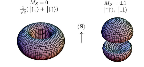
Figure 1: Spin-projected two-body density $\rho^{(2)}_{1,M_{S}}(\bm{r})$ of the deuteron calculated with the AV18 potential. Shown is the iso-density surface for $0.005\;\textrm{fm}^{-3}$.

These structures are the manifestation of two types of interaction-induced correlations which govern the nuclear many-body problem: (i) short-range central correlations and (ii) tensor correlations.

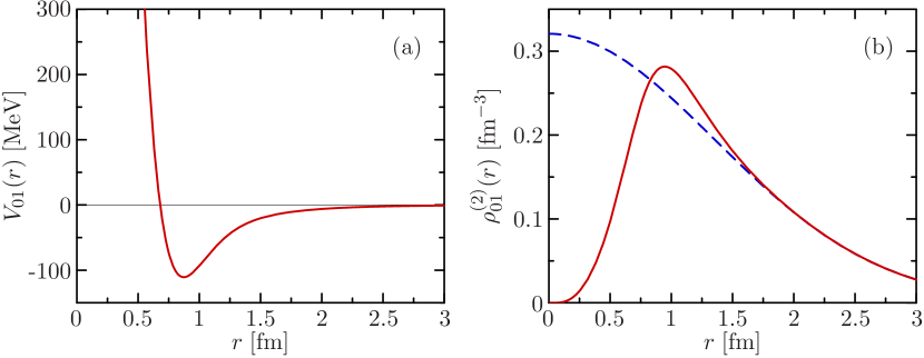
Figure 2: (a) Central part of the AV18 potential in the $(S,T)=(0,1)$ channel. (b) Two-body density distribution $\rho^{(2)}_{S=0,T=1}(\bm{r})$ for ${}^{4}\text{He}$ resulting from an ansatz wave function using a Slater determinant of Gaussian single-particle states () compared to a realistic two-body density including the interaction-induced central correlations ().

The central correlations are induced by the strong repulsive core of the central part of the interaction. Figure 2 shows the radial dependence of the central part of the AV18 potential in a specific spin-isospin channel. Due to the short-range repulsion the two-body density, shown for ${}^{4}\text{He}$, is completely suppressed within the region of the repulsive core. A typical ansatz for the many-body wave function using a Slater determinant of Gaussian (or any other) single-particle states is not capable of describing this correlation hole. The dashed line in Fig. 2(b) shows that the Slater determinant ansatz leads to a significant probability of finding the nucleons within the core. Even with a superposition of a moderate number of Slater determinants one is not able to describe the strong short-range central correlations caused by realistic potentials.

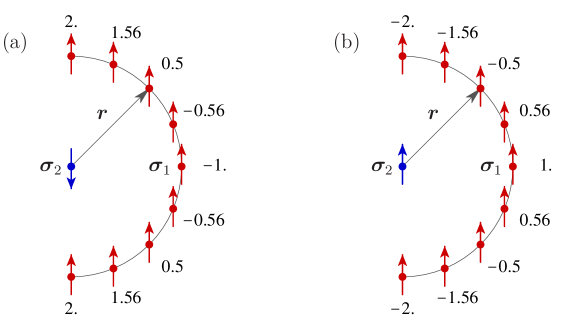
Figure 3: Dependence of the tensor interaction energy on the spatial orientation of the two spins for fixed antiparallel (a) and parallel spins (b), respectively. The numbers indicate the values of $V_{\text{T}}$ for each of the configurations.

The origin of the tensor correlations is the long-range tensor interaction, particularly in the $(S,T)=(1,0)$ channel. As seen in Fig. 1, the tensor correlations are revealed through the dependence of the two-body density on the spatial orientation of the two nucleons with respect to their spins. This can be understood from the structure of the tensor operator $\mathrm{S}_{12}=\frac{3}{\mathrm{r}^{2}}(\bm{\mathrm{\sigma}}_{1}\cdot\bm{\mathrm{r}})(\bm{\mathrm{\sigma}}_{2}\cdot\bm{\mathrm{r}})-(\bm{\mathrm{\sigma}}_{1}\cdot\bm{\mathrm{\sigma}}_{2})$. For illustration we consider the interaction energy $V_{\text{T}}=-[\frac{3}{r^{2}}(\bm{\sigma}_{1}\cdot\bm{r})(\bm{\sigma}_{2}\cdot\bm{r})-(\bm{\sigma}_{1}\cdot\bm{\sigma}_{2})]$, where the minus sign was introduced to account for the sign of the radial dependence of the tensor interaction. Spin vectors and relative coordinate enter in the same way as for the magnetic dipole-dipole interaction. Figure 3 gives the values of $V_{\text{T}}$ for different spatial orientations of two fixed antiparallel and parallel spins, respectively. For antiparallel spins, those configuration with $\bm{r}$ perpendicular to the spin direction are energetically favoured. Contrariwise, for parallel spins a fully aligned arrangement of spins and relative coordinate is preferred. This explains the structure of the two-body density shown in Fig. 1. It is clear that these tensor correlations between the two spins and the relative coordinate cannot be described adequately by a single Slater determinant.

The aim of this paper is to devise and apply a method to include central and tensor correlations explicitly into simple model spaces. We discuss this approach, the Unitary Correlation Operator Method (UCOM), in Sec. 2. The structure of the correlated realistic interaction is presented in Sec. 3 with application to the AV18 potential. Section 4 introduces a simple yet powerful variational model for the treatment of the nuclear many-body problem based on the Slater determinant of Gaussian wave packets used in Fermionic Molecular Dynamics (FMD). Ground state calculations up to mass numbers $A\lesssim 60$ are performed, and binding energies, charge radii, and charge distributions are compared to experiment. Finally, Sec. 5 discusses the projection onto angular momentum eigenstates of the intrinsically deformed variational states and compares the resulting rotational spectra with experiment.

2 Unitary Correlation Operator Method (UCOM)

2.1 Concept

The basic idea of the Unitary Correlation Operator Method (UCOM) is the following: Introduce the dominant short-range central and tensor correlations into a simple many-body state by means of a state-independent unitary transformation. The unitary operator $\mathrm{C}$ describing this transformation applied to an uncorrelated many-body state $\,|{\Psi}\rangle$ leads to a correlated state $\,|{\hat{\Psi}}\rangle$,

$$\,|{\hat{\Psi}}\rangle=\mathrm{C}\;\,|{\Psi}\rangle\;.$$ (1)

In the simplest case, the uncorrelated state is a Slater determinant. The correlated state $\,|{\hat{\Psi}}\rangle$, however, is no longer a Slater determinant. Due to the complex short-range correlations introduced by the correlation operator $\mathrm{C}$, any expansion of $\,|{\hat{\Psi}}\rangle$ in a basis of Slater determinants will require a huge number of basis states.

The representation of short-range correlations in terms of a unitary state-independent operator is technically very advantageous. Calculating a matrix element $\langle{\hat{\Psi}}|\,{\mathrm{O}}\,|{\hat{\Psi}^{\prime}}\rangle$ of an operator $\mathrm{O}$ with correlated states is equivalent to calculating the matrix element $\langle{\Psi}|\,{\hat{\mathrm{O}}}\,|{\Psi^{\prime}}\rangle$ of the correlated operator

$$\hat{\mathrm{O}}={{\mathrm{C}}}^{{\dagger}}\mathrm{O}\,\mathrm{C}$$ (2)

using uncorrelated states. For the treatment of the many-body problem it is generally more convenient to correlate all operators of interest and to evaluate expectation values or matrix elements with the uncorrelated states.

In accord with the two types of correlations discussed above, we decompose the correlation operator into separate unitary operators $\mathrm{C}_{\Omega}$ and $\mathrm{C}_{r}$ for tensor and central correlations, respectively,

$$\mathrm{C}=\mathrm{C}_{\Omega}\mathrm{C}_{r}=\exp\!\Big{[}-\mathrm{i}\sum_{i<j}\mathrm{g}_{\Omega,ij}\Big{]}\;\exp\!\Big{[}-\mathrm{i}\sum_{i<j}\mathrm{g}_{r,ij}\Big{]}\;.$$ (3)

Each of the correlation operators can be written as an exponential involving a Hermitian generator. Since the correlations considered here are induced by a two-body potential, the generators are also assumed to be two-body operators. The detailed form of the two-body generators $\mathrm{g}_{r}$ and $\mathrm{g}_{\Omega}$ reflects the structure of the central and tensor correlations, as discussed in the Sec. 1. We will construct these generators in the following sections.

2.2 Central Correlations

The short-range repulsion in the central part of the NN-interaction prevents the nucleons in a many-body system from approaching each other closer than the extent of the repulsive core, i.e., the two-body density matrix exhibits a correlation hole at small interparticle distances. One way to incorporate these correlations into a simple many-body state is by shifting each pair of nucleons apart from each other. The shift has to be distance-dependent since it should only affect nucleon pairs which are closer than the core radius.

Using this picture, we can construct the following ansatz for the Hermitian generator of the corresponding unitary transformation (3): radial shifts are generated by the component of the relative momentum $\bm{\mathrm{q}}=\frac{1}{2}[\bm{\mathrm{p}}_{1}-\bm{\mathrm{p}}_{2}]$ along the distance vector $\bm{\mathrm{r}}=\bm{\mathrm{x}}_{1}-\bm{\mathrm{x}}_{2}$ of two particles:

$$\mathrm{q}_{r}=\frac{1}{2}[\bm{\mathrm{q}}\cdot\tfrac{\bm{\mathrm{r}}}{\mathrm{r}}+\tfrac{\bm{\mathrm{r}}}{\mathrm{r}}\cdot\bm{\mathrm{q}}]\;.$$ (4)

To describe the dependence of the shift on the particle distance we introduce a function $s(r)$ and define the following Hermitian generator for the central correlation operator $\mathrm{C}_{r}$ [11]:

$$\mathrm{g}_{r}=\frac{1}{2}[s(\mathrm{r})\mathrm{q}_{r}+\mathrm{q}_{r}s(\mathrm{r})]\;.$$ (5)

To illustrate the effect of the correlation operator $\mathrm{c}_{r}=\exp[-\mathrm{i}\mathrm{g}_{r}]$ in two-body space, we apply it to a two-body state $\,|{\psi}\rangle=\,|{\Phi_{\text{cm}}}\rangle\otimes\,|{\phi}\rangle$. The correlation operator does not act on the centre of mass component $\,|{\Phi_{\text{cm}}}\rangle$ by construction. For the correlated relative part $\,|{\hat{\phi}}\rangle$ we obtain in coordinate representation [11]:

$$\langle{\bm{r}}|{\hat{\phi}}\rangle=\langle{\bm{r}}|\,{\mathrm{c}_{r}}\,|{\phi}\rangle=\frac{R_{-}(r)}{r}\sqrt{R^{\prime}_{-}(r)}\;\;\langle{R_{-}(r)\tfrac{\bm{r}}{r}}|{\phi}\rangle\;.$$ (6)

Hence, the application of the correlation operator corresponds to a norm conserving coordinate transformation $\bm{r}\mapsto R_{-}(r)\frac{\bm{r}}{r}$ with respect to the relative coordinate. The function $R_{-}(r)$ and its inverse $R_{+}(r)$ are connected to the shift function $s(r)$ by the integral equation

$$\int_{r}^{R_{\pm}(r)}\frac{\mathrm{d}\xi}{s(\xi)}=\pm 1\;,\qquad R_{\pm}[R_{\mp}(r)]=r\;.$$ (7)

For slowly varying shift functions $s(r)$, the correlation functions are approximately given by $R_{\pm}(r)\approx r\pm s(r)$. The $R_{\pm}(r)$ are determined by an energy minimisation in the two-body system, as discussed in Sec. 3.5.

Since the NN-interaction depends strongly on the spin $S$ and isospin $T$ of the interacting nucleon pair, we decompose the two-body generators $\mathrm{g}_{r}$ into a sum of different generators $\mathrm{g}_{r}^{ST}$ for each of the four different $(S,T)$ channels

$$\mathrm{g}_{r}=\sum_{S,T}\mathrm{g}_{r}^{ST}\mathrm{\Pi}_{ST}\;,$$ (8)

where $\mathrm{\Pi}_{ST}$ is a projection operator onto the spin $S$ and isospin $T$ subspace. The correlation operator in two-body space decomposes into a sum of independent correlation operator for the different channels

$$\mathrm{c}_{r}=\exp\!\Big{[}-\mathrm{i}\sum_{S,T}\mathrm{g}_{r}^{ST}\mathrm{\Pi}_{ST}\Big{]}=\sum_{S,T}\exp[-\mathrm{i}\mathrm{g}_{r}^{ST}]\;\mathrm{\Pi}_{ST}=\sum_{S,T}\mathrm{c}_{r}^{ST}\mathrm{\Pi}_{ST}\;.$$ (9)

This form is very convenient, since it allows us to treat the $(S,T)$ channels separately. For the sake of a concise formulation, we will not write out this spin-isospin dependence in the following, but add it when needed.

2.3 Tensor Correlations

The strong tensor part of the NN-interaction induces subtle correlations between the spin of a nucleon pair and their relative spatial orientation. In order to describe these correlations, we need to generate a spatial shift perpendicular to the radial direction. This is done by the “orbital momentum” operator

$$\bm{\mathrm{q}}_{\Omega}=\bm{\mathrm{q}}-\tfrac{\bm{\mathrm{r}}}{\mathrm{r}}\;\mathrm{q}_{r}=\frac{1}{2\mathrm{r}^{2}}[\,\bm{\mathrm{l}}\times\bm{\mathrm{r}}-\bm{\mathrm{r}}\times\bm{\mathrm{l}}\,]\;,$$ (10)

where $\bm{\mathrm{l}}$ is the relative orbital angular momentum operator. Radial momentum $\tfrac{\bm{\mathrm{r}}}{\mathrm{r}}\mathrm{q}_{r}$ and the orbital momentum $\bm{\mathrm{q}}_{\Omega}$ constitute a special decomposition of the relative momentum operator $\bm{\mathrm{q}}$ and generate shifts orthogonal to each other. The complex dependence of the shift on the spin orientation is encapsulated in the following ansatz for the generator $\mathrm{g}_{\Omega}$ [12]:

$$\mathrm{g}_{\Omega}=\frac{3}{2}\vartheta(\mathrm{r})\big{[}(\bm{\mathrm{\sigma}}_{1}\!\cdot\bm{\mathrm{q}}_{\Omega})(\bm{\mathrm{\sigma}}_{2}\!\cdot\bm{\mathrm{r}})+(\bm{\mathrm{\sigma}}_{1}\!\cdot\bm{\mathrm{r}})(\bm{\mathrm{\sigma}}_{2}\!\cdot\bm{\mathrm{q}}_{\Omega})\big{]}=\vartheta(r)\,\mathrm{s}_{12}(\bm{\mathrm{r}},\bm{\mathrm{q}}_{\Omega})\;,$$ (11)

where $\mathrm{s}_{12}(\bm{\mathrm{r}},\bm{\mathrm{q}}_{\Omega})=\frac{3}{2}[(\bm{\mathrm{\sigma}}_{1}\!\cdot\bm{\mathrm{q}}_{\Omega})(\bm{\mathrm{\sigma}}_{2}\!\cdot\bm{\mathrm{r}})+(\bm{\mathrm{\sigma}}_{1}\!\cdot\bm{\mathrm{r}})(\bm{\mathrm{\sigma}}_{2}\!\cdot\bm{\mathrm{q}}_{\Omega})]$. The two spin operators and the relative coordinate $\bm{\mathrm{r}}$ enter in a similar manner like in the tensor operator $\mathrm{s}_{12}$, however, one of the coordinate operators is replaced by the orbital momentum $\bm{\mathrm{q}}_{\Omega}$, which generates the transverse shift. The size and the distance-dependence of the transverse shift is given by the function $\vartheta(r)$ — the counterpart to $s(r)$ for the central correlator. The isospin dependence of the tensor correlator is implemented in analogy to the spin-isospin dependence of the central correlator (9) through projection operators.

Again we illustrate the effect of the correlation operator $\mathrm{c}_{\Omega}=\exp[-\mathrm{i}\mathrm{g}_{\Omega}]$ by applying it to a two-body wave function in coordinate representation. For simplicity we use $LS$-coupled two-body states $\,|{\phi;(LS)J}\rangle$. Starting from a pure $L=0$ uncorrelated wave function with $S=1$, $T=0$, and $J=1$, for example, the tensor correlator generates a superposition of an $L=0$ and an $L=2$ state

$$\begin{split}\langle{\bm{r}}|\,{\mathrm{c}_{\Omega}}\,|{\phi;(01)1}\rangle=&\cos(3\sqrt{2}\;\vartheta(r))\;\;\langle{\bm{r}}|{\phi;(01)1}\rangle\\ &+\sin(3\sqrt{2}\;\vartheta(r))\;\;\langle{\bm{r}}|{\phi;(21)1}\rangle\;.\end{split}$$ (12)

The tensor correlation function $\vartheta(r)$ determines the amplitude and the radial dependence of the D-wave admixture.

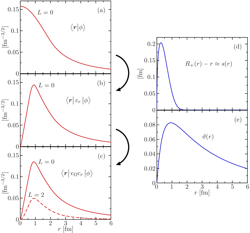
Figure 4: Construction of the deuteron wave function for the AV18 potential starting from an uncorrelated wave function shown in panel (a). Application of the central correlator with a correlation function $R_{+}(r)$ shown in (d) leads to the central correlated wave function (b). Application of the tensor correlator with $\vartheta(r)$ shown in panel (e) produces a D-wave admixture and leads to a realistic deuteron wave function depicted in (c).

To further illustrate the effect of the central and the tensor correlation operator on a two-body state, Fig. 4 details the steps from a simplistic ansatz to the exact deuteron wave function for the AV18 potential. We start with an uncorrelated $L=0$ wave function, shown in panel (a), which correctly describes the long-range behaviour but does not contain a correlation hole or a D-wave admixture. Applying, in a first step, the central correlation operator with the correlation function $R_{+}(r)$ depicted in panel (d) leads to the correlated wave function shown in Fig. 4(b). The amplitude is shifted out of the core region towards particle distances where the potential is attractive. To this end, the shift function $s(r)\approx R_{+}(r)-r$ has to be large within the core radius, but has to decrease rapidly outside the core region. In a second step, we apply the tensor correlator for a correlation function $\vartheta(r)$ given in Fig. 4(e). As seen from Eq. (12) this generates a D-wave admixture and leads to a fully correlated wave function depicted in panel (c), which is in nice agreement with the exact deuteron solution. Note that the shape of the $D$-wave component is determined by the correlation function $\vartheta(r)$ — a long-range $L=2$ wave function requires a tensor correlation function $\vartheta(r)$ of long range.

2.4 Correlated Operators and Cluster Expansion

The explicit formulation of correlated wave functions for the many-body problem becomes technically increasingly complicated, and the equivalent notion of correlated operators proves more convenient. The similarity transformation (2) of an operator $\mathrm{O}$ leads to a correlated operator which contains irreducible contributions to all particle numbers. We can formulate a cluster expansion of the correlated operator

$$\hat{\mathrm{O}}={{\mathrm{C}}}^{{\dagger}}\mathrm{O}\mathrm{C}=\hat{\mathrm{O}}^{[1]}+\hat{\mathrm{O}}^{[2]}+\hat{\mathrm{O}}^{[3]}+\cdots\;,$$ (13)

where $\hat{\mathrm{O}}^{[n]}$ denotes the irreducible $n$-body part [11]. When starting with a $k$-body operator, all irreducible contributions $\hat{\mathrm{O}}^{[n]}$ with $n<k$ vanish. Hence, the unitary transformation of a two-body operator — the NN-interaction for example — yields a correlated operator containing a two-body contribution, a three-body term, etc.

The significance of the higher order terms depends on the range of the central and tensor correlations [11, 12, 14]. If the range of the correlation functions is small compared to the mean interparticle distance, then three-body and higher-order terms of the cluster expansion are negligible. Discarding these higher-order contributions leads to the two-body approximation

$$\hat{\mathrm{O}}^{C2}=\hat{\mathrm{O}}^{[1]}+\hat{\mathrm{O}}^{[2]}\;.$$ (14)

Already the example discussed in connection with Fig. 4 shows that for the central correlations the two-body approximation is well justified. The range of the shift function $s(r)\approx R_{+}(r)-r$ is smaller than the mean interparticle distance at saturation density which is about $1.8\,\text{fm}$. One can show by an explicit evaluation [14] that higher order contributions due to central correlations are indeed small for the nuclear many-body problem.

The situation is different for tensor correlations. The tensor correlation function $\vartheta(r)$ needed to generate the D-wave component of the deuteron wave function is necessarily long-ranged (see Fig. 4(e)). In a many-nucleon system, however, the tensor correlations between two nucleons will not be established up to the same large distances as in the deuteron. The other nucleons interfere and inhibit the formation of long-range tensor correlations and thus lead to an effective screening of the long-range tensor correlations. If we were to use the long-range tensor correlator suitable for the deuteron also in the many-body problem, this screening effect would emerge through substantial higher-order contributions of the cluster expansion. Since an explicit calculation of the higher-order tensor contributions to the cluster expansion is presently not feasible, we will anticipate the screening of the long-range tensor correlations by restricting the range of the tensor correlation function [12]. In this way, we can improve upon the quality of the computationally simple two-body approximation. Possible residual long-range tensor correlations that are not represented in the short-range tensor correlator have to be described by the many-body states of the model space. We will come back to the construction of the optimal correlation functions for a given NN-potential in Sec. 3.5.

3 Correlated Realistic Interactions

3.1 Nuclear Hamiltonian

We are now applying the formalism of the Unitary Correlation Operator Method discussed in Sec. 2 to construct the correlated nuclear Hamiltonian in two-body approximation. The starting point is an uncorrelated Hamiltonian for the $A$-body system

$$\mathrm{H}=\mathrm{T}+\mathrm{V}=\sum_{i=1}^{A}\frac{1}{2m_{N}}\,\bm{\mathrm{p}}_{i}^{2}+\sum_{i>j=1}^{A}\mathrm{v}_{ij}\;,$$ (15)

consisting of the kinetic energy operator $\mathrm{T}$ and a two-body potential $\mathrm{V}$. For the latter, we employ realistic NN-potentials from the Bonn or Argonne family of interactions. Those are given in a closed operator representation facilitating the use within the UCOM framework. The Argonne V14 [15] and the charge independent terms of the Argonne V18 interaction [1] have the following operator structure

$$\begin{split}\mathrm{v}_{\text{Argonne}}&=\sum_{S,T}\big{[}v_{ST}^{c}(\mathrm{r})+v_{ST}^{l2}(\mathrm{r})\;\bm{\mathrm{l}}\,{}^{2}\big{]}\;\mathrm{\Pi}_{ST}\\ &+\sum_{T}\big{[}v_{T}^{t}(\mathrm{r})\;\mathrm{s}_{12}+v_{T}^{ls}(\mathrm{r})\;(\bm{\mathrm{l}}\cdot\bm{\mathrm{s}})+v_{T}^{ls2}(\mathrm{r})\;(\bm{\mathrm{l}}\cdot\bm{\mathrm{s}})^{2}\big{]}\;\mathrm{\Pi}_{1T}\;,\end{split}$$ (16)

where $\mathrm{\Pi}_{ST}$ denotes the projection operator onto spin $S$ and isospin $T$. In the following, operators $\mathrm{\Pi}_{S}$ with a single index always refer to a projection in spin-space only. The quadratic spin-orbit term can be rewritten

$$(\bm{\mathrm{l}}\cdot\bm{\mathrm{s}})^{2}=\tfrac{2}{3}\bm{\mathrm{l}}\,{}^{2}\mathrm{\Pi}_{1}-\tfrac{1}{2}(\bm{\mathrm{l}}\cdot\bm{\mathrm{s}})+\tfrac{1}{6}\mathrm{s}_{12}(\bm{\mathrm{l}},\bm{\mathrm{l}})\;,$$ (17)

where

$$\mathrm{s}_{12}(\bm{\mathrm{l}},\bm{\mathrm{l}})=3(\bm{\mathrm{\sigma}}_{1}\cdot\bm{\mathrm{l}})(\bm{\mathrm{\sigma}}_{2}\cdot\bm{\mathrm{l}})-(\bm{\mathrm{\sigma}}_{1}\cdot\bm{\mathrm{\sigma}}_{2})\,\bm{\mathrm{l}}{\,}^{2}\;.$$ (18)

The non-relativistic configuration space versions of the Bonn potentials [2] are parametrised using a different set of operators

$$\begin{split}\mathrm{v}_{\text{Bonn}}&=\sum_{S,T}\big{[}v_{ST}^{c}(\mathrm{r})+\tfrac{1}{2}\{\bm{\mathrm{q}}^{2}v_{ST}^{q2}(\mathrm{r})+v_{ST}^{q2}(\mathrm{r})\,\bm{\mathrm{q}}^{2}\}\big{]}\;\mathrm{\Pi}_{ST}\\ &+\sum_{T}\big{[}v_{T}^{t}(\mathrm{r})\;\mathrm{s}_{12}+v_{T}^{ls}(\mathrm{r})\;(\bm{\mathrm{l}}\cdot\bm{\mathrm{s}})\big{]}\;\mathrm{\Pi}_{1T}\;.\end{split}$$ (19)

Instead of the $\bm{\mathrm{l}}\,{}^{2}$ and $(\bm{\mathrm{l}}\cdot\bm{\mathrm{s}})^{2}$ terms in (16), the Bonn potentials employ a non-local momentum-dependent term involving $\bm{\mathrm{q}}^{2}$. For the following considerations it is convenient to rephrase this contribution in terms of the radial momentum $\mathrm{q}_{r}$ and the angular momentum $\bm{\mathrm{l}}$

$$\tfrac{1}{2}\{\bm{\mathrm{q}}^{2}v^{q2}(\mathrm{r})+v^{q2}(\mathrm{r})\,\bm{\mathrm{q}}^{2}\}=\tfrac{1}{2}\{\mathrm{q}_{r}^{2}v^{q2}(\mathrm{r})+v^{q2}(\mathrm{r})\,\mathrm{q}_{r}^{2}\}+\frac{v^{q2}(\mathrm{r})}{\mathrm{r}^{2}}\;\bm{\mathrm{l}}\,{}^{2}\;.$$ (20)

3.2 Tensor Correlated Hamiltonian

The first step to construct the correlated Hamiltonian in two-body approximation is the application of the tensor correlation operator $\mathrm{c}_{\Omega}=\exp(-\mathrm{i}\mathrm{g}_{\Omega})$ in two-body space. A general way to evaluate the similarity transformation is by utilising the Baker-Campbell-Hausdorff expansion

$$\begin{split}{{\mathrm{c}}}^{{\dagger}}_{\Omega}\mathrm{O}\,\mathrm{c}_{\Omega}&=\exp(\mathrm{i}\mathrm{g}_{\Omega})\mathrm{O}\exp(-\mathrm{i}\mathrm{g}_{\Omega})\\ &=\mathrm{O}+\mathrm{i}\;[{\mathrm{g}_{\Omega}},{\mathrm{O}}]+\frac{\mathrm{i}^{2}}{2}[{\mathrm{g}_{\Omega}},{[{\mathrm{g}_{\Omega}},{\mathrm{O}}]}]+\cdots\\ &=\sum_{n=0}^{\infty}\frac{1}{n!}\mathsf{L}_{\Omega}^{n}\;\mathrm{O}=\exp(\mathsf{L}_{\Omega})\,\mathrm{O}\;.\end{split}$$ (21)

In the last line we have introduced a compact notation of the iterated commutators in terms of powers of the super-operator $\mathsf{L}_{\Omega}\,\circ=\mathrm{i}[{\mathrm{g}_{\Omega}},{\circ}]$ with the generator $\mathrm{g}_{\Omega}$ given by Eq. (11). Summing up the full expansion formally leads to the exponential of the super-operator.

First we study the transformation of the various terms of the realistic NN-potentials (16) and (19). A minimal set of operators we have to consider in order to formulate the tensor correlated interaction is $\{\mathrm{r},\mathrm{q}_{r}^{2},\bm{\mathrm{l}}\,{}^{2},(\bm{\mathrm{l}}\cdot\bm{\mathrm{s}}),\mathrm{s}_{12},\mathrm{s}_{12}(\bm{\mathrm{l}},\bm{\mathrm{l}})\}$. The distance operator $\mathrm{r}$ commutes with the generator $\mathrm{g}_{\Omega}$, i.e., it is invariant under tensor correlations

$${{\mathrm{c}}}^{{\dagger}}_{\Omega}\mathrm{r}\,\mathrm{c}_{\Omega}=\mathrm{r}\;.$$ (22)

For the radial momentum $\mathrm{q}_{r}^{2}$, the Baker-Campbell-Hausdorff expansion terminates after the second order and we obtain a closed expression for the tensor correlated operator [12],

$${{\mathrm{c}}}^{{\dagger}}_{\Omega}\mathrm{q}_{r}^{2}\mathrm{c}_{\Omega}=\mathrm{q}_{r}^{2}-[\vartheta^{\prime}(\mathrm{r})\,\mathrm{q}_{r}+\mathrm{q}_{r}\vartheta^{\prime}(\mathrm{r})]\;\mathrm{s}_{12}(\bm{\mathrm{r}},\bm{\mathrm{q}}_{\Omega})+[\vartheta^{\prime}(\mathrm{r})\;\mathrm{s}_{12}(\bm{\mathrm{r}},\bm{\mathrm{q}}_{\Omega})]^{2}\;,$$ (23)

which can be further simplified using the identity $\mathrm{s}_{12}(\bm{\mathrm{r}},\bm{\mathrm{q}}_{\Omega})^{2}=9[\bm{\mathrm{s}}^{2}+3(\bm{\mathrm{l}}\cdot\bm{\mathrm{s}})+(\bm{\mathrm{l}}\cdot\bm{\mathrm{s}})^{2}]$. All other basic operators require the evaluation of the full commutator expansion (21). At first order, the following commutators appear [16]:

$$\begin{split}[{\mathrm{g}_{\Omega}},{\mathrm{s}_{12}}]&=\mathrm{i}\vartheta(\mathrm{r})[-24\,\mathrm{\Pi}_{1}-18\,(\bm{\mathrm{l}}\cdot\bm{\mathrm{s}})+3\,\mathrm{s}_{12}]\\ [{\mathrm{g}_{\Omega}},{(\bm{\mathrm{l}}\cdot\bm{\mathrm{s}})}]&=\mathrm{i}\vartheta(\mathrm{r})[-\bar{\mathrm{s}}_{12}(\bm{\mathrm{q}}_{\Omega},\bm{\mathrm{q}}_{\Omega})]\\ [{\mathrm{g}_{\Omega}},{\bm{\mathrm{l}}\,{}^{2}}]&=\mathrm{i}\vartheta(\mathrm{r})[2\,\bar{\mathrm{s}}_{12}(\bm{\mathrm{q}}_{\Omega},\bm{\mathrm{q}}_{\Omega})]\\ [{\mathrm{g}_{\Omega}},{\mathrm{s}_{12}(\bm{\mathrm{l}},\bm{\mathrm{l}})}]&=\mathrm{i}\vartheta(\mathrm{r})[7\,\bar{\mathrm{s}}_{12}(\bm{\mathrm{q}}_{\Omega},\bm{\mathrm{q}}_{\Omega})]\;,\end{split}$$ (24)

where we have used the short-hand notation

$$\bar{\mathrm{s}}_{12}(\bm{\mathrm{q}}_{\Omega},\bm{\mathrm{q}}_{\Omega})=2\mathrm{r}^{2}\mathrm{s}_{12}(\bm{\mathrm{q}}_{\Omega},\bm{\mathrm{q}}_{\Omega})+\mathrm{s}_{12}(\bm{\mathrm{l}},\bm{\mathrm{l}})-\tfrac{1}{2}\,\mathrm{s}_{12}\;.$$ (25)

In addition to the original set of operators, a new tensor containing two orbital momentum operators is generated

$$\mathrm{s}_{12}(\bm{\mathrm{q}}_{\Omega},\bm{\mathrm{q}}_{\Omega})=3(\bm{\mathrm{\sigma}}_{1}\cdot\bm{\mathrm{q}}_{\Omega})(\bm{\mathrm{\sigma}}_{2}\cdot\bm{\mathrm{q}}_{\Omega})-(\bm{\mathrm{\sigma}}_{1}\cdot\bm{\mathrm{\sigma}}_{2})\,\bm{\mathrm{q}}_{\Omega}^{2}\;.$$ (26)

For the calculation of the second order of the expansion (21), the commutator of $\mathrm{g}_{\Omega}$ and $\bar{\mathrm{s}}_{12}(\bm{\mathrm{q}}_{\Omega},\bm{\mathrm{q}}_{\Omega})$ is required:

$$[{\mathrm{g}_{\Omega}},{\bar{\mathrm{s}}_{12}(\bm{\mathrm{q}}_{\Omega},\bm{\mathrm{q}}_{\Omega})}]=\mathrm{i}\vartheta(\mathrm{r})[(108+96\bm{\mathrm{l}}\,{}^{2})\mathrm{\Pi}_{1}+(153+36\bm{\mathrm{l}}\,{}^{2})(\bm{\mathrm{l}}\cdot\bm{\mathrm{s}})+15\mathrm{s}_{12}(\bm{\mathrm{l}},\bm{\mathrm{l}})]\;.$$ (27)

Again a new operator, $\bm{\mathrm{l}}\,{}^{2}(\bm{\mathrm{l}}\cdot\bm{\mathrm{s}})$, emerges, whose commutator with the generator enters into the third order of the Baker-Campbell-Hausdorff expansion:

$$[{\mathrm{g}_{\Omega}},{\bm{\mathrm{l}}\,{}^{2}(\bm{\mathrm{l}}\cdot\bm{\mathrm{s}})}]=\mathrm{i}\vartheta(\mathrm{r})[-3\;\bar{\mathrm{s}}_{12}(\bm{\mathrm{q}}_{\Omega},\bm{\mathrm{q}}_{\Omega})-\{{\bm{\mathrm{l}}\,{}^{2}\bar{\mathrm{s}}_{12}(\bm{\mathrm{q}}_{\Omega},\bm{\mathrm{q}}_{\Omega})}\}_{\text{H}}]\;.$$ (28)

This in turn leads to the new operator $\{{\bm{\mathrm{l}}\,{}^{2}\bar{\mathrm{s}}_{12}(\bm{\mathrm{q}}_{\Omega},\bm{\mathrm{q}}_{\Omega})}\}_{\text{H}}=\frac{1}{2}(\bm{\mathrm{l}}\,{}^{2}\bar{\mathrm{s}}_{12}(\bm{\mathrm{q}}_{\Omega},\bm{\mathrm{q}}_{\Omega})+\bar{\mathrm{s}}_{12}(\bm{\mathrm{q}}_{\Omega},\bm{\mathrm{q}}_{\Omega})\bm{\mathrm{l}}\,{}^{2})$, whose commutator appears in the fourth order of the expansion:

$$\begin{split}[{\mathrm{g}_{\Omega}},{\{{\bm{\mathrm{l}}\,{}^{2}\bar{\mathrm{s}}_{12}(\bm{\mathrm{q}}_{\Omega},\bm{\mathrm{q}}_{\Omega})}\}_{\text{H}}}]=&\mathrm{i}\vartheta(\mathrm{r})[324\mathrm{\Pi}_{1}+477(\bm{\mathrm{l}}\cdot\bm{\mathrm{s}})+600\bm{\mathrm{l}}\,{}^{2}+51\mathrm{s}_{12}(\bm{\mathrm{l}},\bm{\mathrm{l}})\\ &+477\bm{\mathrm{l}}\,{}^{2}(\bm{\mathrm{l}}\cdot\bm{\mathrm{s}})+144\bm{\mathrm{l}}{\,}^{4}+27\bm{\mathrm{l}}\,{}^{2}\mathrm{s}_{12}(\bm{\mathrm{l}},\bm{\mathrm{l}})+36\bm{\mathrm{l}}{\,}^{4}(\bm{\mathrm{l}}\cdot\bm{\mathrm{s}})]\;.\end{split}$$ (29)

Evidently, with increasing order in the Baker-Campbell-Hausdorff expansion, operators containing successively higher powers of the angular momentum $\bm{\mathrm{l}}$ are generated. The last three terms of (29) are of fourth order in $\bm{\mathrm{l}}$ already. In the following, we will neglect the contributions beyond the third order in angular momentum. Thus we achieve a closure of the operator set contributing to the Baker-Campbell-Hausdorff expansion:

$$\begin{split}\{\mathrm{r},\mathrm{q}_{r}^{2},&\bm{\mathrm{l}}\,{}^{2},(\bm{\mathrm{l}}\cdot\bm{\mathrm{s}}),\mathrm{s}_{12},\mathrm{s}_{12}(\bm{\mathrm{l}},\bm{\mathrm{l}}),\\ &\bar{\mathrm{s}}_{12}(\bm{\mathrm{q}}_{\Omega},\bm{\mathrm{q}}_{\Omega}),\mathrm{q}_{r}\mathrm{s}_{12}(\bm{\mathrm{r}},\bm{\mathrm{q}}_{\Omega}),\{{\bm{\mathrm{l}}\,{}^{2}\bar{\mathrm{s}}_{12}(\bm{\mathrm{q}}_{\Omega},\bm{\mathrm{q}}_{\Omega})}\}_{\text{H}},\bm{\mathrm{l}}\,{}^{2}(\bm{\mathrm{l}}\cdot\bm{\mathrm{s}})\}\;.\end{split}$$ (30)

We can represent the super-operator $\mathsf{L}_{\Omega}$ defined in (21) as a matrix acting on the vector (30) of operators. The summation of the full Baker-Campbell-Hausdorff expansion is then reduced to calculating a matrix exponential for the super-operator. In this way a closed operator representation of the tensor correlated potential is constructed.

The set (30) already contains the operators relevant for the transformation of the kinetic energy. We can decompose the kinetic energy $\mathrm{T}$ in two-body space into a relative, $\mathrm{t}_{\text{rel}}$, and a centre of mass contribution, $\mathrm{t}_{\text{cm}}$. The latter is not affected by the correlations. The relative contribution is further decomposed into a radial and an angular term

$$\mathrm{T}=\mathrm{t}_{\text{cm}}+\mathrm{t}_{\text{rel}}=\mathrm{t}_{\text{cm}}+\frac{1}{m_{N}}\Big{(}\mathrm{q}_{r}^{2}+\frac{\bm{\mathrm{l}}\,{}^{2}}{\mathrm{r}^{2}}\Big{)}\;.$$ (31)

Thus the transformation of the kinetic energy can be inferred from the transformation properties of the first three operators in the set (30).

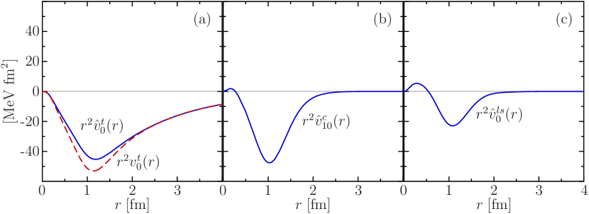
Figure 5: Radial dependency of the tensor part of the AV18 potential () and the radial dependencies () of the tensor (a), central (b), and spin-orbit contribution (c) that result from applying the tensor correlator to the isolated tensor part of the interaction. All potentials are for the $(S,T)=(1,0)$ channel, and the appropriate tensor correlation function is given in Sec. 3.5 ($\alpha$-correlators).

The effect of the tensor correlator on the tensor part of the interaction is illustrated in Fig. 5. For this example we take the isolated tensor part of the AV18 potential in the $(S,T)=(1,0)$ channel and apply the tensor correlation operator. Through the correlation procedure, i.e., the application of the matrix exponential according to (21), contributions to the other operator channels (30) are generated. Most notably, additional central and spin-orbit contributions emerge, which are depicted in panels (b) and (c) of Fig. 5. Both, the induced central and spin-orbit contributions are attractive at intermediate ranges. Hence, through the correlation procedure, part of the tensor attraction is transfered to other operator channels, where it can be exploited using simple uncorrelated many-body states. The marginal repulsion at short ranges will be completely removed by the central correlation operator as discussed in the following.

3.3 Central and Tensor Correlated Hamiltonian

The subsequent application of the central correlator to the tensor correlated terms of Hamiltonian is technically simpler. In Section 2.2 we have shown that the central correlator acts like a norm conserving coordinate transformation when applied to a relative two-body wave function (6). Using the transformation properties of the wave function in coordinate representation we can immediately derive expressions for the central-correlated operators in two-body approximation [11]. The evaluation of the Baker-Campbell-Hausdorff expansion for the central correlations is therefore not required.

The application of the central correlation operator $\mathrm{c}_{r}$ to the distance operator $\mathrm{r}$ confirms the picture of a coordinate transformation

$${{\mathrm{c}}}^{{\dagger}}_{r}\mathrm{r}\,\mathrm{c}_{r}=R_{+}(\mathrm{r})\;,$$ (32)

where $R_{+}(r)$ is the correlation function introduced in Sec. 2.2. Wherever the distance operator $\mathrm{r}$ appears in the Hamiltonian, it has to be replaced by a transformed distance operator $R_{+}(\mathrm{r})$. This affects, most notably, all radial dependencies of the different contributions of the interaction

$${{\mathrm{c}}}^{{\dagger}}_{r}v(\mathrm{r})\,\mathrm{c}_{r}=v\big{(}R_{+}(\mathrm{r})\big{)}\;.$$ (33)

The components of the relative momentum operator $\bm{\mathrm{q}}$ are also influenced by the central correlations. Using the correlated two-body wave function (6), one can show that

$${{\mathrm{c}}}^{{\dagger}}_{r}\mathrm{q}_{r}\mathrm{c}_{r}=\frac{1}{\sqrt{R^{\prime}_{+}(\mathrm{r})}}\,\mathrm{q}_{r}\,\frac{1}{\sqrt{R^{\prime}_{+}(\mathrm{r})}}\;,\qquad{{\mathrm{c}}}^{{\dagger}}_{r}\bm{\mathrm{q}}_{\Omega}\mathrm{c}_{r}=\frac{\mathrm{r}}{R_{+}(\mathrm{r})}\bm{\mathrm{q}}_{\Omega}\;.$$ (34)

For the quadratic radial momentum $\mathrm{q}_{r}^{2}$, which appears in the tensor correlated potential as well as in the kinetic energy (31), one obtains

$${{\mathrm{c}}}^{{\dagger}}_{r}\mathrm{q}_{r}^{2}\mathrm{c}_{r}=\frac{1}{2}\Big{\{}\frac{1}{[R^{\prime}_{+}(\mathrm{r})]^{2}}\mathrm{q}_{r}^{2}+\mathrm{q}_{r}^{2}\frac{1}{[R^{\prime}_{+}(\mathrm{r})]^{2}}\Big{\}}+\frac{7[R^{\prime\prime}_{+}(\mathrm{r})]^{2}}{4[R^{\prime}_{+}(\mathrm{r})]^{4}}-\frac{R^{\prime\prime\prime}_{+}(\mathrm{r})}{2[R^{\prime}_{+}(\mathrm{r})]^{3}}\;.$$ (35)

Notice that the transformation of $\mathrm{q}_{r}^{2}$ generates a local potential in addition to the momentum-dependent term.

All basic operators that act only on the angular part of the two-body wave function, are invariant under central correlations, e.g.,

$${{\mathrm{c}}}^{{\dagger}}_{r}\bm{\mathrm{l}}\,\mathrm{c}_{r}=\bm{\mathrm{l}}\;,\qquad{{\mathrm{c}}}^{{\dagger}}_{r}\frac{\bm{\mathrm{r}}}{\mathrm{r}}\mathrm{c}_{r}=\frac{\bm{\mathrm{r}}}{\mathrm{r}}\;.$$ (36)

Utilising the unitarity of the correlation operator, one can easily deduce from these basic identities the correlated expressions for the composite tensor and spin orbit operators contained in the operator set (30). One finds that $\bm{\mathrm{l}}\,{}^{2}$, $(\bm{\mathrm{l}}\cdot\bm{\mathrm{s}})$, $\mathrm{s}_{12}$, $\mathrm{s}_{12}(\bm{\mathrm{l}},\bm{\mathrm{l}})$, $\bar{\mathrm{s}}_{12}(\bm{\mathrm{q}}_{\Omega},\bm{\mathrm{q}}_{\Omega})$, $\{{\bm{\mathrm{l}}\,{}^{2}\bar{\mathrm{s}}_{12}(\bm{\mathrm{q}}_{\Omega},\bm{\mathrm{q}}_{\Omega})}\}_{\text{H}}$, and $\bm{\mathrm{l}}\,{}^{2}(\bm{\mathrm{l}}\cdot\bm{\mathrm{s}})$ are invariant under similarity transformation with the central correlation operator.

3.4 Properties of the Correlated Interaction $\mathrm{V}_{\textup{UCOM}}$

Combining the different central and tensor correlated operators discussed in the previous sections, we can formulate the correlated many-body Hamiltonian in two-body approximation

$$\hat{\mathrm{H}}^{C2}=\hat{\mathrm{T}}^{[1]}+\hat{\mathrm{T}}^{[2]}+\hat{\mathrm{V}}^{[2]}=\mathrm{T}+\mathrm{V}_{\textrm{UCOM}}\;.$$ (37)

Its one-body contribution is just the uncorrelated kinetic energy $\hat{\mathrm{T}}^{[1]}=\mathrm{T}$. Two-body contributions arise from the correlated kinetic energy $\hat{\mathrm{T}}^{[2]}$ and the correlated potential $\hat{\mathrm{V}}^{[2]}$. Together they constitute the correlated interaction $\mathrm{V}_{\textrm{UCOM}}$, which is the basis for the following nuclear structure studies.

The generic operator structure of the correlated interaction $\mathrm{V}_{\textrm{UCOM}}$ is more complicated than that of the bare potentials

$$\begin{split}\mathrm{v}_{\textrm{UCOM}}&=\sum_{S,T}\big{[}\hat{v}_{ST}^{c}(\mathrm{r})+\{\hat{v}_{ST}^{qr2}(\mathrm{r})\,\mathrm{q}_{r}^{2}\}_{H}+\hat{v}_{ST}^{l2}(\mathrm{r})\,\bm{\mathrm{l}}\,{}^{2}\big{]}\;\mathrm{\Pi}_{ST}\\ &+\sum_{T}\big{[}\hat{v}_{T}^{ls}(\mathrm{r})\,(\bm{\mathrm{l}}\cdot\bm{\mathrm{s}})+\hat{v}_{T}^{t}(\mathrm{r})\,\mathrm{s}_{12}+\hat{v}_{T}^{tll}(\mathrm{r})\,\mathrm{s}_{12}(\bm{\mathrm{l}},\bm{\mathrm{l}})\\ &\qquad+\hat{v}_{T}^{tqq}(\mathrm{r})\,\bar{\mathrm{s}}_{12}(\bm{\mathrm{q}}_{\Omega},\bm{\mathrm{q}}_{\Omega})+\hat{v}_{T}^{l2tqq}(\mathrm{r})\,\{{\bm{\mathrm{l}}\,{}^{2}\bar{\mathrm{s}}_{12}(\bm{\mathrm{q}}_{\Omega},\bm{\mathrm{q}}_{\Omega})}\}_{\text{H}}\\[6.0pt] &\qquad+\{{\hat{v}_{T}^{qr2trq}(\mathrm{r})\,\mathrm{q}_{r}^{2}\,\mathrm{s}_{12}(\bm{\mathrm{r}},\bm{\mathrm{q}}_{\Omega})}\}_{\text{H}}+\hat{v}_{T}^{l2ls}(\mathrm{r})\,\bm{\mathrm{l}}\,{}^{2}(\bm{\mathrm{l}}\cdot\bm{\mathrm{s}})\big{]}\;\mathrm{\Pi}_{1T}\;,\end{split}$$ (38)

where we use the short-hand notation $\{{\cdots}\}_{\text{H}}$ to indicate explicit Hermitisation. The new radial dependencies $\hat{v}_{ST}^{\,\cdots}(r)$ result from the correlation procedure, i.e., from the matrix exponential for the tensor correlator and the coordinate transformation for the central correlator. They depend on the radial dependencies of the bare potential and on the correlation functions. The structure of the different radial dependencies was discussed in Refs. [11, 12]. In summary, the two prime effects of the unitary transformation are: (i) The short-range repulsive core of the central interaction is removed by the central correlator and an effective repulsion in the momentum-dependent terms is generated. (ii) Additional attractive central and spin-orbit contributions as well as new tensorial terms are created by the tensor correlator out of the bare tensor interaction.

Before entering into concrete many-body calculations, we summarise a few key properties of the correlated interaction $\mathrm{V}_{\textrm{UCOM}}$. First, the correlated interaction is phase-shift equivalent to the uncorrelated potential by construction. This is a direct consequence of the finite range of the correlation functions. The asymptotics of a scattering wave function is not altered by the correlation operators and the phase shifts are preserved. Hence, the unitary correlation operator provides a tool to generate an infinite manifold of phase-shift equivalent NN-potentials originating from a single realistic interaction. In addition to the two-body potential the correlation operator generates a three-body (and higher-order) interaction which, of course, depends on the particular correlation functions used.

Furthermore, there is an interesting connection to the low-momentum interaction $V_{\text{low}-k}$ determined by means of renormalisation group techniques [17]. The momentum space matrix elements of $\mathrm{V}_{\textrm{UCOM}}$ are in very good agreement with the $V_{\text{low}-k}$ matrix elements [12]. Although both approaches are formally quite different, the underlying physics is the same: the high-momentum components of the interaction are treated explicitly — by the unitary correlation operator or through the renormalisation group procedure — leaving an effective interaction adapted to low-momentum model spaces. One major practical advantage of the correlated interaction $\mathrm{V}_{\textrm{UCOM}}$ is that it is given in a closed operator representation (38). Depending on the particular application, one can easily compute the relevant matrix elements, e.g., in a plane wave, oscillator, or non-orthogonal Gaussian basis. The renormalisation group method just provides numerical values for the momentum-space matrix elements.

3.5 Optimal Correlation Functions

A crucial step is the construction of optimal correlation functions for the use in many-body calculations. These correlation functions depend, of course, on the bare potential, but they should not depend on the nucleus under consideration. The aim is to fix a set of optimal state-independent correlation functions which define a fixed correlated interaction $\mathrm{V}_{\textrm{UCOM}}$. When constructing the correlation functions one, therefore, has to disentangle state-dependent properties and state-independent features.

This is an issue in particular for the tensor correlations in the $(S,T)=(1,0)$ channel. The long-range tensor correlation function $\vartheta(r)$, which was used in Fig. 4(e) to reproduce the D-wave admixture of the exact deuteron solution, is certainly not appropriate for a many-body system. As already discussed in Sec. 2.4, long-range tensor correlations of a pair of nucleons are screened through tensor interactions with other nucleons. One way to isolate the essential state-independent contributions is to restrict the tensor correlation functions to short ranges. Long-range tensor correlations, which are not accounted for explicitly by the short-range correlator, have to be described through the degrees of freedom of the many-body states. For the central correlations this restriction to short ranges emerges automatically, since the strong repulsive core and the induced correlation hole are short-ranged themselves.

Another motivation to consider only correlation functions of short range is the validity of the two-body approximation. The two-body approximation is appropriate as long as the correlation range is small compared to the mean interparticle distance. In this case, the probability of finding three nucleons within the range of the correlator is sufficiently small to neglect three-body and higher-order contributions to the cluster expansion.

Different methods for the construction of optimal correlation functions were discussed in detail in Refs. [11, 12]. Here we employ an energy minimisation in the two-body system using simple parametrisations for the central and tensor correlation functions. For the correlation functions $R_{+}(r)$ in the four possible $(S,T)$ channels we will use one of the following forms:

$$\begin{split}R_{+}^{A}(r)&=r+\alpha\,(r/\beta)^{\eta}\exp[-\exp(r/\beta)]\;,\\ R_{+}^{B}(r)&=r+\alpha\,(1-\exp[-(r/\gamma)^{\eta}])\exp[-\exp(r/\beta)]\;.\end{split}$$ (39)

The tensor correlations functions $\vartheta(r)$ for the two $S=1$ channels are parametrised by

$$\begin{split}\vartheta^{A}(r)&=\alpha\,(1-\exp[-(r/\gamma)^{\eta}])\exp[-\exp(r/\beta)]\;,\\ \vartheta^{B}(r)&=\alpha\,(1-\exp[-(r/\gamma)^{\eta}])\exp[-r/\beta]\;.\end{split}$$ (40)

The uncorrelated two-body wave functions are the free zero-energy solutions of the two-body Schrödinger equation with the lowest orbital angular momentum consistent with antisymmetry for given $(S,T)$. The energy minimisation is performed for each $(S,T)$ channel separately. The range of the tensor correlation function in the $(S,T)=(1,0)$ channel is controlled by using the following integral constraint for the variation

$$\int\mathrm{d}{r}\;r^{2}\vartheta(r)=\begin{cases}0.1\,\text{fm}^{3}&;\alpha\text{-correlator}\\ 0.5\,\text{fm}^{3}&;\gamma\text{-correlator}\\ \end{cases}\;.$$ (41)

Depending on this constraint on the $(S,T)=(1,0)$ tensor correlation functions, we will refer to the resulting sets of correlators as $\alpha$- and $\gamma$-correlators, respectively. The parameters of the correlation functions resulting from the energy minimisation for the AV18 potential are summarised in Table 1. The details of their determination and the corresponding correlation functions for the Bonn A potential can be found in Ref. [12].

Table 1: Parameters of the optimal central and tensor correlation functions for the AV18 potential as determined in Ref. [12].

Central correlation functions $R_{+}(r)$
$(S,T)$	Param.	$\alpha\;\text{[fm]}$	$\beta\;\text{[fm]}$	$\gamma\;\text{[fm]}$	$\eta$
$(0,1)$	A	1.379	0.8854	—	0.3723
$(1,0)$	A	1.296	0.8488	—	0.4187
$(0,0)$	B	0.76554	1.272	0.4243	1
$(1,1)$	B	0.57947	1.3736	0.1868	1
Tensor correlation functions $\vartheta(r)$
$(S,T)$	Param.	$\alpha$	$\beta\;\text{[fm]}$	$\gamma\;\text{[fm]}$	$\eta$
$(1,0)\alpha$	A	530.38	1.298	1000	1
$(1,0)\gamma$	A	0.383555	2.665	0.4879	1
$(1,1)$	B	-0.023686	1.685	0.8648	1

Plots of the optimal correlation functions for the AV18 potential are shown in Fig. 6. All central correlation functions $R_{+}(r)-r$ are of similar short range. Beyond $r\approx 1.5\,\text{fm}$ for the even channels and $r\approx 2\,\text{fm}$ for the odd channels the shift $R_{+}(r)-r$ vanishes and the unitary correlation operator acts like the identity operator. In general, the maximum shift is smaller for the odd channels, since the uncorrelated $L=1$ wave functions are already depleted at small $r$ by the centrifugal barrier. The tensor correlation function $\vartheta(r)$ in the $(S,T)=(1,1)$ channel is very weak and does not lead to significant effects. For the dominant $(S,T)=(1,0)$ channel, the optimal tensor correlators for the two different values of the constraint (41) are depicted. Only the $\alpha$-correlator can be considered short-ranged. The $\gamma$-correlator has sizable contributions beyond $3\,\text{fm}$ and one has to expect significant three-body contributions to the cluster expansion.

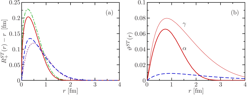
Figure 6: Optimal central (a) and tensor correlation functions (b) for the AV18 potential. The different lines correspond to the different $(S,T)$ channels: $(0,1)$ (), $(1,0)$ (), $(0,0)$ (), $(1,1)$ ().

An indirect estimate for higher-order contributions to the cluster expansion can be obtained by comparing the exact solution of a few-body problem using the correlated Hamiltonian in two-body approximation with the solution based on the bare interaction. This has been done in the no-core shell model [8] for ${}^{4}\text{He}$ [18]. It turns out that for the $\alpha$-correlators the three- and four-body contributions to the correlated Hamiltonian are roughly $4\;\text{MeV}$. For the longer ranged $\gamma$-correlators this contribution grows significantly.

4 Variational Ground State Calculations

The correlated realistic interaction $\mathrm{V}_{\textrm{UCOM}}$ provides a robust starting point for different approaches to tackle the many-body problem. The dominant short-range correlations are included explicitly though the unitary correlation operator so that simple low-momentum many-body spaces — not able to represent the short-range correlations themselves — suffice for a realistic description.

4.1 Variational Model — FMD States

Here we will employ a variational model based on an extremely versatile parametrisation for the many-body states which was developed in the framework of the Fermionic Molecular Dynamics (FMD) model [19, 20, 21, 22]. The many-body trial state $\,|{Q}\rangle$ is given by a Slater determinant of single-particle states $\,|{q_{i}}\rangle$

$$\,|{Q}\rangle=\mathcal{A}(\,|{q_{1}}\rangle\otimes\,|{q_{2}}\rangle\otimes\cdots\otimes\,|{q_{A}}\rangle)\;.$$ (42)

The single-particle states $\,|{q}\rangle$ are parametrised by Gaussian wave packets with variable spin orientation and fixed isospin. In general a superposition of several wave packets can be used to represent the single-nucleon state

$$\,|{q}\rangle=\sum_{\nu=1}^{n}c_{\nu}\;\,|{a_{\nu},\bm{b}_{\nu}}\rangle\otimes\,|{\chi_{\nu}}\rangle\otimes\,|{m_{t}}\rangle\;.$$ (43)

The Gaussian wave packet in configuration space is parametrised in terms of a complex width parameter $a_{\nu}$ and a complex vector $\bm{b}_{\nu}=\bm{\rho}_{\nu}+\mathrm{i}a_{\nu}\bm{\pi}_{\nu}$, where $\bm{\rho}_{\nu}$ is the mean position and $\bm{\pi}_{\nu}$ the mean momentum of the wave packet,

$$\langle{\bm{x}}|{a_{\nu},\bm{b}_{\nu}}\rangle=\exp\!\Big{[}-\frac{(\bm{x}-\bm{b}_{\nu})^{2}}{2a_{\nu}}\Big{]}\;.$$ (44)

In the simplest case each single particle-state contains $10$ independent variational parameters. These are determined by a large-scale numerical minimisation of the expectation value of the correlated Hamiltonian

$$E=\frac{\langle{Q}|\,{\hat{\mathrm{H}}^{C2}-\mathrm{T}_{\text{cm}}}\,|{Q}\rangle}{\langle{Q}|{Q}\rangle}\to\text{min.}$$ (45)

The operator $\mathrm{T}_{\text{cm}}$ of the centre of mass kinetic energy is explicitly subtracted to eliminate the centre of mass contribution to the energy.

The antisymmetrised Gaussian trial states are extremely flexible and allow for a multitude of intrinsic structures. Shell-model type states as well as states with strong $\alpha$-clustering can be described on the same footing. One should stress that in the following calculations none of these structures is put in by hand, but that they emerge naturally from the energy minimisation. A tremendous technical advantage is that all necessary matrix elements, e.g., for the various terms of the correlated interaction, can be calculated analytically. This makes large-scale variational calculations up to mass numbers $A\approx 60$ possible. Details on the matrix elements and the implementation are given in Ref. [23].

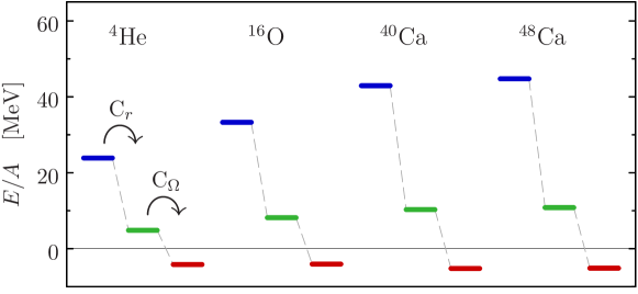
Figure 7: Energy expectation value for different nuclei calculated with the uncorrelated Hamiltonian (left), the central-correlated Hamiltonian (centre) and the fully correlated Hamiltonian (right) in two-body approximation using the $\alpha$-correlators.

We use this variational model to illustrate the effect of the central and tensor correlations on the ground-state energy of different nuclei. To this end we perform the energy minimisation with the fully correlated interaction (38) using the $\alpha$-correlators. With the resulting states we then compute the expectation values of the central-correlated Hamiltonian (without tensor correlations) and of the uncorrelated Hamiltonian. The results for ${}^{4}\text{He}$, ${}^{16}\text{O}$, ${}^{40}\text{Ca}$, and ${}^{48}\text{Ca}$ are summarised in Fig. 7. The energy expectation value calculated with the uncorrelated Hamiltonian is large and positive, i.e., the system is not bound. As discussed in Sec. 1 the Slater determinant (42) is not capable of describing short-range central and tensor correlations. This entails that the repulsive core of the central interaction generates a large positive energy contribution and that the expectation value of the tensor part is practically zero.

The proper inclusion of the short-range central correlations lowers the energy significantly, but still does not lead to bound nuclei since the attractive contribution of the tensor interaction is missing. This is a striking demonstration of the importance of the tensor interaction and the associated correlations. Only after the inclusion of both, central and tensor correlation operators, we obtain bound ground-states.

We point out that in general all tensor components of the correlated interaction $\mathrm{V}_{\textrm{UCOM}}$ detailed in (38) yield negligible expectation values with a single Slater determinant and can be omitted in the following. The tensor interaction enters only though the central, the $\bm{\mathrm{l}}\,{}^{2}$, and the $(\bm{\mathrm{l}}\cdot\bm{\mathrm{s}})$ terms generated by the correlation procedure (cf. Sec. 3.2). For the sake of simplicity, the $\bm{\mathrm{l}}\,{}^{2}(\bm{\mathrm{l}}\cdot\bm{\mathrm{s}})$ contribution in (38) is replaced by $2(\bm{\mathrm{l}}\cdot\bm{\mathrm{s}})$ and added to the conventional $(\bm{\mathrm{l}}\cdot\bm{\mathrm{s}})$ term. Thus two-body states with $L=0$ and $L=1$ are treated correctly and contributions from $L\geq 2$ components, which are suppressed due to the centrifugal barrier, are approximated.

4.2 Long-Range Correlations and Three-Body Interactions

Table 2: Variational ground state energies and charge radii for the correlated AV18 potential with the $\alpha$- and $\gamma$-correlators in comparison with experiment.

	AV18$\alpha$		AV18$\gamma$		Experiment
Nucleus	$E/A\;[\text{MeV}]$	$r_{\text{ch}}\;[\text{fm}]$	$E/A\;[\text{MeV}]$	$r_{\text{ch}}\;[\text{fm}]$	$E/A\;[\text{MeV}]$	$r_{\text{ch}}\;[\text{fm}]$
${}^{4}\text{He}$	-4.18	1.57	-6.99	1.51	-7.07	1.68
${}^{16}\text{O}$	-4.07	2.33	-7.40	2.25	-7.98	2.71
${}^{28}\text{Si}$	-3.45	2.72	-6.68	2.66	-8.45	3.12
${}^{40}\text{Ca}$	-5.22	2.87	-8.19	2.89	-8.55	3.48
${}^{48}\text{Ca}$	-5.14	2.87	-7.87	2.93	-8.67	3.47

In the framework of the FMD variational model we calculate the ground state energies and the charge radii for a few nuclei using the correlated AV18 potential with the short-ranged $\alpha$-correlators. Table 2 summarises the results and compares them to experimental data. The magnitude of the binding energies and the charge radii for larger nuclei are significantly smaller than the experimental values. There are two major reasons for these systematic deviations: long-range correlations and genuine three-body forces.

Long-range correlations. Due to the restriction of the range of the tensor correlator in the $(S,T)=(1,0)$ channel, long-range tensor correlations are not adequately described by the correlator. Remember, the range constraint is used in order to ensure the validity of the two-body approximation (cf. Sec. 3.5). Ideally, the missing long-range correlations would have to be accounted for by the model-space. However, in the case of the simple variational model, the single Slater determinant is not capable of describing long-range tensor correlations. In principle one could enlarge the model-space such that the long-range attraction provided by the tensor interaction can be exploited. This would lead to an increase in binding energy and radius but is presently not feasible, at least for larger nuclei.

Alternatively one could resort to long-range tensor correlators at the price of including contributions of higher orders of the cluster expansion. A step into this direction is the use of the longer-ranged $\gamma$-correlator in the $(S,T)=(1,0)$ channel. The binding energies and charge radii resulting in two-body approximation are also given in Tab. 2. The binding energy increases significantly compared to the $\alpha$-correlators. Part of this increase is an artifact of the two-body approximation: The three-body contributions, which are neglected here, would provide an effective repulsion and compensate most of the gain in binding energy. Hence, a treatment of long-range tensor correlations by the Unitary Correlations Operator necessitates a consistent inclusion of higher-order cluster contributions — a technically extremely challenging task.

Genuine three-body forces. As quasi-exact Green’s function Monte Carlo calculations for small systems show [5], realistic two-body potentials alone do not generate sufficient binding to reproduce experimental data. This can be remedied by introducing a phenomenological three-nucleon force which is adjusted to ground states and low-lying excitations [9]. Promising developments in effective field theories [10] might lead to realistic three-body forces which go beyond the rather phenomenological three-body terms considered so far in ab initio calculations.

4.3 Phenomenological Correction

The inclusion of three body terms, a genuine three-body force or three-body contributions of the cluster expansion, poses an enormous computational challenge. At the moment this is not feasible for the full range of particle numbers envisioned. We, therefore, resort to a pragmatic approach and employ a momentum-dependent two-body force to simulate the missing three-body terms and long-range correlations. The generic contribution of a momentum-dependent two-body interaction to the energy per particle in nuclear matter is similar to a local three-body force.

The structure of the phenomenological correction should be as simple as possible. For the single Slater determinant employed so far, only the local and momentum-dependent central terms and the spin-orbit term have sizable contributions. Therefore, a sensible ansatz for the correction is a sum of these three terms

$$\Delta\mathrm{v}=\Delta v^{c}(\mathrm{r})+\bm{\mathrm{q}}\,\Delta v^{qq}(\mathrm{r})\,\bm{\mathrm{q}}+\Delta v^{ls}(\mathrm{r})\,(\bm{\mathrm{l}}\cdot\bm{\mathrm{s}})\;.$$ (46)

The symmetric form of the momentum-dependent part is chosen for convenience and can easily be transformed to the form appearing in (38) or (19). In order to keep the correction simple we consider only spin-isospin independent, i.e., Wigner-type, forces. Each of the radial dependencies $\Delta v(r)$ is given by a single Gauss function

$$\Delta v(r)=\gamma\exp[-r^{2}/(2\kappa)]$$ (47)

with strength $\gamma$ and range parameter $\kappa$. The adjustment of the parameters of the three radial dependencies is done in two steps: First, the strengths and ranges of the central corrections are adjusted such that binding energies and charge radii of the doubly magic nuclei ${}^{4}\text{He}$, ${}^{16}\text{O}$, and ${}^{40}\text{Ca}$ are in agreement with experiment. Notice that there are only four parameters available to fit six quantities. Second, the parameters of the attractive spin-orbit correction are chosen such that the binding energies of ${}^{24}\text{O}$ and ${}^{48}\text{Ca}$ are consistent with experiment. The resulting correction parameters for the correlated AV18 potential with the short-ranged $\alpha$-correlators are

$$\begin{array}[]{r l l}\Delta v^{c}(r):&\gamma=-7.261\;\text{MeV},&\kappa=2.75\;\text{fm}^{2}\;,\\ \Delta v^{qq}(r):&\gamma=+14.05\;\text{MeV}\,\text{fm}^{2},&\kappa=2.5\;\text{fm}^{2}\;,\\ \Delta v^{ls}(r):&\gamma=-2.7\;\text{MeV},&\kappa=3.0\;\text{fm}^{2}\;.\end{array}$$ (48)

It turns out that each of the three terms of the correction plays a different and physically quite intuitive role. The repulsive momentum-dependent term is responsible for the reduction of the central densities and the increase of the charge radii. The attractive local term provides the bulk of the missing binding energy. The attractive spin-orbit term gives additional binding especially for nuclei far off stability. Hence, (46) can be considered the simplest possible form of correction capable of generating all the necessary effects.

One of the effects which is absorbed in the phenomenological correction is the lack of long-range tensor correlations. From this it is already clear that the correction depends on the available model space. For an extended model space, which is capable of describing part of the missing correlations by itself, the phenomenological correction will be different. The parameter set (48) is adapted to a model space of states consisting of a single Slater determinant as used in our variational approach or in Hartree-Fock calculations. If one allows for superpositions of Slater determinants, e.g., in the framework of variation after projection or multi-configuration calculations, the correction has to be readjusted.

4.4 Binding Energies and Charge Radii

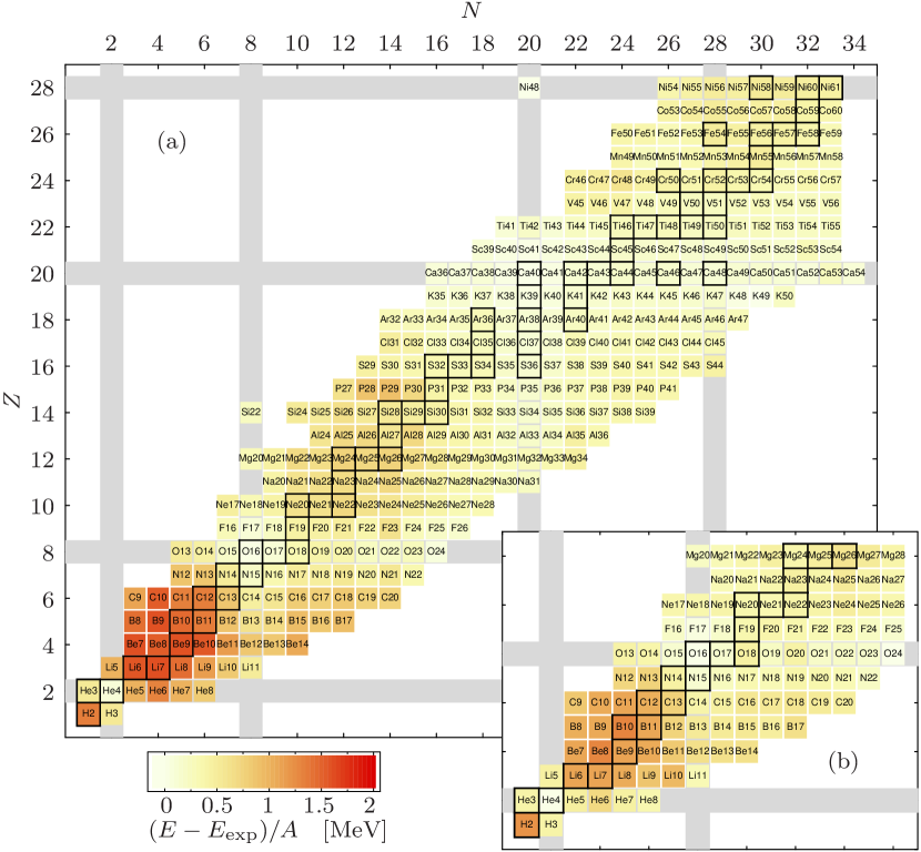
Figure 8: Chart of nuclei accessible to the variational model. The shading shows the difference between the variational and the experimental binding energy. The main chart (a) was obtained using a single Gaussian wave packet per nucleon. The inset (b) shows results with two Gaussians per nucleon.

Using the $\alpha$-correlated AV18 potential with the phenomenological correction (46) we perform variational ground state calculations in the mass region $A\lesssim 60$. Figure 8 depicts the part of the nuclear chart accessible to the variational model based on the FMD trial state (42). The shadings indicate the deviation of the energy expectation value (45) from the experimental binding energy per nucleon [24]. The main chart was obtained using a single Gaussian wave packet to describe the single-particle states. The agreement with experiment of the absolute binding energies around the magic numbers and for larger nuclei is quite good (bright shades). The largest deviations appear for $p$- and $sd$-shell nuclei away from the shell closures. One reason for these deviations is the insufficient flexibility of the single-particle trial states to simulate, e.g., the long-range behaviour of the states especially for light nuclei. Enhancing the flexibility by using a superposition of two Gaussians to parametrise the single-particle states leads to a significant improvement, as the small chart in Fig. 8 demonstrates.

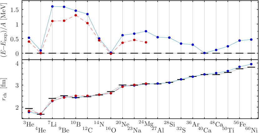
Figure 9: Difference between variational and experimental binding energy per nucleon (upper panel) and charge radius (lower panel) for selected stable isotopes. All calculations are performed using the $\alpha$-correlated AV18 potential plus phenomenological correction (46). Shown are results obtained with one () and with two Gaussian wave-packets () for each single-particle trial state.

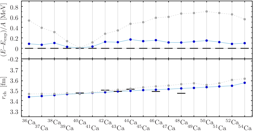
Figure 10: Binding energy difference and charge radius for Calcium isotopes (cf. Fig. 9). Depicted are results based on the $\alpha$-correlated AV18 potential with the full phenomenological correction () and with the central terms of the correction only ().

A more quantitative view is given in Fig. 9, where the binding energy deviations $(E-E_{\text{exp}})/A$ and the charge radii $r_{\text{ch}}$ are shown for selected stable isotopes. The calculated charge radii are in excellent agreement with the experimental data [25] throughout the whole mass range. The binding energies are in nice agreement with experiment in the vicinity of the magic nuclei but start to deviate in between the shell closures, especially for $p$-shell nuclei. As already mentioned, part of this deviation is due to an insufficient flexibility of the single-particle trial states. A refinement of the trial states by using a superposition of two Gaussian wave-packets (dashed line) instead of one (solid line) leads to a noticeable improvement of the energies. The remaining discrepancy can be reduced further by angular momentum projection as discussed in Sec. 5.

For larger nuclei, the trial state with one Gaussian per nucleon provides a good description. The binding energy differences and charge radii for the Calcium isotopes are depicted in Fig. 10. The binding energies are in very good agreement with experiment, the charge radii are slightly overestimated for the heavier isotopes but are generally in agreement with experiment. Figure 10 also illustrates the effect of the spin-orbit contribution in the phenomenological correction. The gray symbols show results of a calculation using the $\alpha$-correlated AV18 potential with central correction but without the spin-orbit term. The spin-orbit term provides additional attraction for the $N\neq Z$ isotopes and reduces the charge radii at the same time. The closed-shell $N=Z$ nuclei are not affected.

4.5 Intrinsic Single-Particle Density Distributions

Since the variational calculation provides us with the full many-body wave function we can easily compute other physical quantities, e.g., the intrinsic single-particle density distribution

$$\rho(\bm{x})=\sum_{m_{s},m_{t}}\langle{Q}|\,{{{\mathrm{\Psi}}}^{{\dagger}}_{m_{s},m_{t}}(\bm{x})\mathrm{\Psi}_{m_{s},m_{t}}(\bm{x})}\,|{Q}\rangle\;.$$ (49)

Unlike for the two-particle density distribution, the short-range central and tensor correlations have only marginal influence on the diagonal elements of the one-particle density matrix [11, 14]. Therefore, we restrict ourselves to the uncorrelated one-body densities for simplicity.

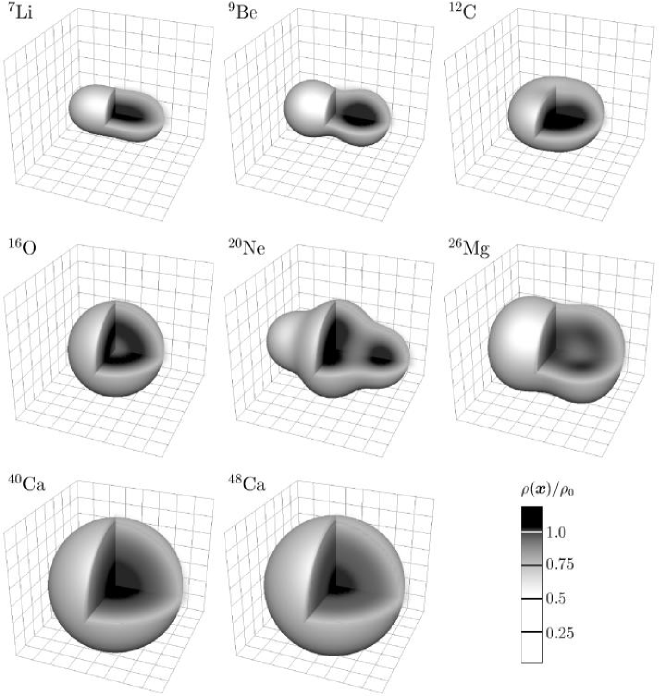
Figure 11: Intrinsic total density distributions of several stable nuclei. Shown is the iso-density surface for $\rho(\bm{x})=\rho_{0}/2$ with one octant cut away to reveal the density distribution in the centre. The colour coding on the section gives the density according to the colour bar at the right. The background grid has a mesh size of $1\,\text{fm}\times 1\,\text{fm}$.

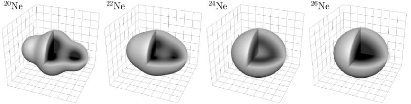
Figure 12: Intrinsic single-particle density distribution $\rho(\bm{x})$ for different Neon isotopes (cf. Fig. 11).

Figure 11 shows three-dimensional illustrations of the intrinsic density distributions for selected nuclei. Depicted is the iso-density surface for $\rho(\bm{x})=\rho_{0}/2$, where $\rho_{0}=0.17\;\text{fm}^{-3}$ is the nuclear matter saturation density. In addition one octant is removed to visualise the interior density distribution. For the doubly magic nuclei ${}^{16}\text{O}$, ${}^{40}\text{Ca}$, and ${}^{48}\text{Ca}$ the variational calculation leads to spherical symmetric density distributions in accord with shell-model-type states. For the $p$- and $sd$-shell nuclei ${}^{7}\text{Li}$, ${}^{9}\text{Be}$, ${}^{12}\text{C}$, ${}^{20}\text{Ne}$, and ${}^{26}\text{Mg}$ the one-body density distributions exhibit pronounced intrinsic deformations. The density distribution of ${}^{9}\text{Be}$ reveals a clear two-$\alpha$ substructure; ${}^{20}\text{Ne}$ shows a toroidal belt similar to a ${}^{12}\text{C}$ nucleus supplemented with two $\alpha$-clusters forming end-caps. For ${}^{26}\text{Mg}$ only remnants of $\alpha$-clustering are visible in the rather smooth density distribution with a multipolar deformation.

These plots showcase the flexibility of the FMD states. A Slater determinant of Gaussian single-particle states is capable of describing shell-model wave functions as well as states with strong $\alpha$-clustering. We should stress that the structures shown in Fig. 11 are generated by a subtle interplay between the different terms of the realistic potential. They are not imposed through constraining the trial state like in $\alpha$-cluster models.

In many cases, strong intrinsic deformations and $\alpha$-clusters present in a $N\approx Z$ nucleus dissolve gradually when neutrons are added (or removed). An example are the Neon isotopes depicted in Fig. 12. Starting from ${}^{20}\text{Ne}$ with its characteristic intrinsic deformation, the addition of neutrons washes out the $\alpha$-clusters and eventually leads to an almost spherical, shell-model-type density distribution for ${}^{26}\text{Ne}$.

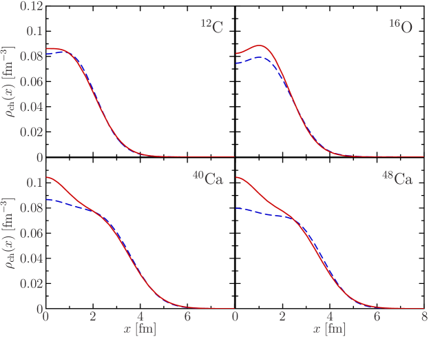
Figure 13: Radial charge distribution $\rho_{\text{ch}}(x)$ for different nuclei obtained from the variational wave function () in comparison with the experimental charge distribution () resulting from a model-independent analysis [25].

Finally, in Fig. 13 we compare the radial charge density distributions for ${}^{12}\text{C}$, ${}^{16}\text{O}$, ${}^{40}\text{Ca}$, and ${}^{48}\text{Ca}$ with a model-independent analysis of electron scattering data [25]. For this comparison, the exact centre of mass correction and the proton and neutron form factors are included in the theoretical curves. The calculated density profiles are in good agreement with the experimental analysis. The surface structure is reproduced extremely well. In the interior the modulations of the calculated density distribution are slightly more pronounced. This behaviour is common to most models based on a single Slater determinant for the ground state; one possibility to improve upon this are multi-configuration calculations. Furthermore, the uncertainties in the experimental determination of the density profiles are largest in this region.

5 Angular Momentum Projection

5.1 Projection after Variation

Many of the density distributions presented in Sec. 4.5 reveal pronounced intrinsic deformations. Evidently the states obtained by energy minimisation for the trial state (42) are not necessarily angular momentum eigenstates as it is the case for the eigenstates of the Hamiltonian — they have to be interpreted as intrinsic states. One can extract angular momentum eigenstates $\,|{\Psi_{JM}}\rangle$ from the intrinsic state $\,|{Q}\rangle$ by a standard angular momentum projection technique [26]. The angular momentum projected states are defined through

$$\,|{\Psi_{JM}}\rangle=\sum_{K}g_{K}^{J}\,\mathrm{P}_{MK}^{J}\,\,|{Q}\rangle\;.$$ (50)

The generalised projection operator $\mathrm{P}_{MK}^{J}$ is given by

$$\mathrm{P}_{MK}^{J}=\frac{2J+1}{8\pi^{2}}\int\mathrm{d}\omega\;D^{J\star}_{MK}(\bm{\omega})\;\mathrm{R}(\bm{\omega})\;,$$ (51)

where $D^{J}_{MK}(\bm{\omega})$ are the Wigner $D$-functions and $\mathrm{R}(\bm{\omega})$ is the unitary rotation operator expressed in terms of the three Euler angles $\bm{\omega}=(\alpha,\beta,\gamma)$:

$$\mathrm{R}(\bm{\omega})=\exp(-\mathrm{i}\alpha\mathrm{J}_{z})\exp(-\mathrm{i}\beta\mathrm{J}_{y})\exp(-\mathrm{i}\gamma\mathrm{J}_{z})\;.$$ (52)

The coefficients $g_{K}^{J}$ are formally determined by minimising the energy expectation value in the projected state $\,|{\Psi_{JM}}\rangle$

$$E_{J}=\frac{\langle{\Psi_{JM}}|\,{\mathrm{H}-\mathrm{T}_{\textrm{cm}}}\,|{\Psi_{JM}}\rangle}{\langle{\Psi_{JM}}|{\Psi_{JM}}\rangle}=\frac{\sum_{KK^{\prime}}g_{K}^{J\star}g_{K^{\prime}}^{J}h_{KK^{\prime}}^{J}}{\sum_{KK^{\prime}}g_{K}^{J\star}g_{K^{\prime}}^{J}n_{KK^{\prime}}^{J}}\;,$$ (53)

where $h_{KK^{\prime}}^{J}=\langle{Q}|\,{(\mathrm{H}-\mathrm{T}_{\textrm{cm}})\mathrm{P}_{KK^{\prime}}^{J}}\,|{Q}\rangle$ and $n_{KK^{\prime}}^{J}=\langle{Q}|\,{\mathrm{P}_{KK^{\prime}}^{J}}\,|{Q}\rangle$. This leads to a generalised eigenvalue problem for the energies $E_{J}$ of the projected states and the coefficients $g_{K}^{J}$:

$$\sum_{K^{\prime}}h_{KK^{\prime}}^{J}\,g_{K^{\prime}}^{J}=E_{J}\sum_{K^{\prime}}n_{KK^{\prime}}^{J}\,g_{K^{\prime}}^{J}\;.$$ (54)

In this paper we employ the angular momentum projection in the framework of a projection after variation (PAV) calculation, i.e., we use the intrinsic state $\,|{Q}\rangle$ obtained by minimising the energy expectation value (45) and subsequently project it onto angular momentum eigenstates (50).

This scheme is different from a variation after projection (VAP) calculation which is based on a minimisation of the energy expectation value (53) calculated with the projected states. The presence of strong intrinsic deformations is associated with a kinetic energy contribution that makes such states unfavourable when minimising the intrinsic energy. This energy contribution, however, is removed by the projection procedure. Therefore, clustering and intrinsic deformation are generally more pronounced in a VAP framework, where the projected energy is minimised. In terms of the available model-space, a VAP calculation goes beyond the variation with a single Slater determinant. The VAP trial state is a specific superposition of rotated Slater determinants. As discussed in Sec. 4.3 this, in general, necessitates a readjustment of the phenomenological correction. First results of a variation after parity projection calculation are available. A full variation after angular momentum projection is computationally extremely involved and will be discussed elsewhere.

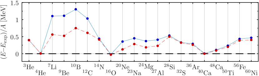
Figure 14: Energy deviation $(E-E_{\text{exp}})/A$ for the intrinsic variational states () and for the angular momentum projected intrinsic states (projection after variation) (). For $A\leq 28$ single-particle states composed of two Gaussians are used, heavier isotopes are calculated with one Gaussian per nucleon.

The effect of the angular momentum projection on the ground state energy is illustrated in Fig. 14, where the intrinsic energies are compared to the energy of the lowest angular momentum eigenstate obtained in the PAV framework. The deviation from the experimental binding energies is reduced by a factor $0.5$ for the intrinsically deformed $p$- and $sd$-shell nuclei. The energy of spherical nuclei is not affected. The residual difference has to be accounted for by further extending the model space, e.g., in the framework of a multi-configuration calculation.

5.2 Rotational Spectra

Besides the ground state the PAV procedure provides us with a whole rotational spectrum based on the intrinsically deformed variational state. Figure 15 shows spectra obtained by angular momentum projection of the intrinsic states for ${}^{7}\text{Li}$, ${}^{9}\text{Be}$, ${}^{12}\text{C}$, and ${}^{20}\text{Ne}$. To give an impression of the influence of the phenomenological correction to the $\alpha$-correlated AV18 potential, three different calculations are shown for each nucleus. First, the $\alpha$-correlated AV18 potential is used without correction term (left column in each panel). As discussed in Sec. 4.2 binding energies and charge radii are generally too small in this case. Nevertheless, the relative spectrum agrees very well with the experimental one. This is a remarkable result, considering that for the rotational band the moment of inertia and thus the radius of the intrinsic density distribution is crucial.

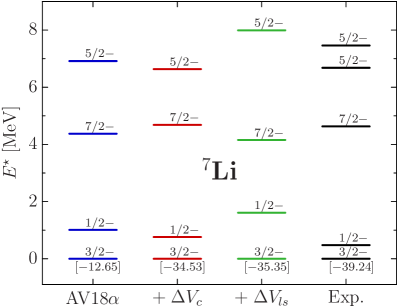
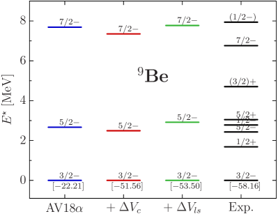
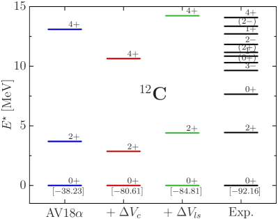
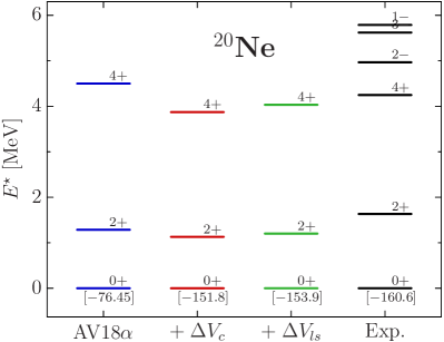
Figure 15: Energy spectra resulting from the angular momentum projection of the variational ground states for ${}^{7}\text{Li}$, ${}^{9}\text{Be}$, ${}^{12}\text{C}$, and ${}^{20}\text{Ne}$. Shown are the excitation energies obtained using the $\alpha$-correlated AV18 potential without correction (first column), with central correction only (second column), with central and spin-orbit correction (third column) in comparison to the experimental spectra (fourth column). The numbers given beneath the lowest level are the absolute ground state energies in $[\text{MeV}]$.

Second, we perform the variation and projection with the $\alpha$-correlated AV18 potential including only the central part of the phenomenological correction (46). Compared to the significant influence of the correction on the binding energy and the radius of the ground state the effect on the spectrum is minor (cf. second column in each of the panels in Fig. 15). Generally the spectra are slightly compressed due to the increase of the radii induced by the central part of the phenomenological correction. The inclusion of the spin-orbit part of the correction stretches the rotational bands again (see third columns in Fig. 15).

Overall, the agreement with experimental data is very encouraging. The ground state rotational bands of ${}^{12}\text{C}$ and ${}^{20}\text{Ne}$ are reproduced very well. Further improvements are possible in the framework of multi-configuration calculations, where some of the missing states corresponding to collective modes can also be described [27].

6 Summary and Outlook

We have combined two powerful tools for the treatment of the nuclear many-body problem: the Unitary Correlation Operator Method (UCOM) and the Fermionic Molecular Dynamics (FMD) model.

The Unitary Correlation Operator Method (UCOM) provides a systematic way to derive, from realistic NN-potentials, effective interactions suitable for simple (low-momentum) model-spaces. Dominant central and tensor correlations induced by the NN-potential are described explicitly by an unitary transformation. By applying the unitary correlation operator to a simple many-body state, e.g., a Slater determinant, the short-range correlations are imprinted into the state. Alternatively the Hamiltonian (and all other operators) can be transformed. The resulting correlated interaction $\mathrm{V}_{\textrm{UCOM}}$ possesses a closed operator representation, is phase-shift equivalent to the original potential, and leads to momentum-space matrix elements in accord with the $V_{\text{low}-k}$ matrix elements [12]. It provides a robust starting point for many-body methods relying on model spaces not capable of describing short-range correlations themselves, e.g., variational models with simple trial states, Hartree-Fock calculations, and multi-configuration shell-model.

We have employed the correlated interaction $\mathrm{V}_{\textrm{UCOM}}$ in the variational framework of the Fermionic Molecular Dynamics (FMD) model. The many-body trial state is a Slater determinant of Gaussian single-particle states which prove to be extremely flexible. On the same footing, it allows for the description of spherical shell-model-type wave functions as well as states with intrinsic deformations and $\alpha$-clustering. At the same time, the approach is computationally quite efficient so that a treatment of nuclei up to mass number $A\lesssim 60$ is possible for realistic two-body interactions with complex operator structure. The inclusion of three-body forces would substantially increase the computational cost and thus reduce the accessible region of the nuclear chart. At the present stage, three-body interactions and long-range correlations are, therefore, simulated by a phenomenological two-body correction. Charge radii and charge distributions are in nice agreement with experiment. Around the magic numbers the variational energies agree well with the experimental binding energies. Away from the shell closures the intrinsic density distributions exhibit strong deformations and $\alpha$-clustering, which necessitates projection of the intrinsic states onto angular momentum eigenstates. Within a projection after variation (PAV) framework we have achieved very promising results for ground state energies and rotational spectra.

Natural next steps are variation after projection (VAP) and multi-configuration calculations. First results along these lines have been obtained using a Generator Coordinate Method to implement an approximate VAP scheme. Constraints on the multipole moments are used to generate different intrinsic states which serve as input for variation after projection (w.r.t. the generator coordinates, i.e., the multipole moments) and multi-configuration calculations. VAP calculations for ${}^{16}\text{O}$ show, e.g., that a tetrahedron of $\alpha$-clusters is energetically more favourable than the spherical shell-model-type state resulting from the unprojected variation [27]. Detailed results of these investigations will be discussed in a forthcoming publication.

Other future applications of the correlated realistic interaction $\mathrm{V}_{\textrm{UCOM}}$ are Hartree-Fock and RPA calculations. This provides a consistent scheme to perform nuclear structure calculations based on realistic NN-potentials also for large nuclei.

References

- [1] R. B. Wiringa, V. G. J. Stoks, R. Schiavilla, Phys. Rev. C 51 (1995) 38.
- [2] R. Machleidt, Adv. Nucl. Phys. 19 (1989) 189.
- [3] R. Machleidt, Phys. Rev. C 63 (2001) 024001.
- [4] V. G. J. Stoks, R. A. M. Klomp, C. P. F. Terheggen, J. J. de Swart, Phys. Rev. C 49 (1993) 2950.
- [5] S. C. Pieper, K. Varga, R. B. Wiringa, Phys. Rev. C 66 (2002) 044310.
- [6] B. S. Pudliner, V. R. Pandharipande, J. Carlson, S. C. Pieper, R. B. Wiringa, Phys. Rev. C 56 (1997) 1720.
- [7] E. Caurier, P. Navrátil, W. E. Ormand, J. P. Vary, Phys. Rev. C 66 (2002) 024314.
- [8] P. Navrátil, J. P. Vary, B. R. Barrett, Phys. Rev. C 62 (2000) 054311.
- [9] S. C. Pieper, V. R. Pandharipande, R. B. Wiringa, Phys. Rev. C 64 (2001) 014001.
- [10] D. R. Entem, R. Machleidt, Phys. Rev C. 68 (2003) 041001.
- [11] H. Feldmeier, T. Neff, R. Roth, J. Schnack, Nucl. Phys. A632 (1998) 61.
- [12] T. Neff, H. Feldmeier, Nucl. Phys. A714 (2003) 311.
- [13] J. L. Forest, V. R. Pandharipande, S. C. Pieper, R. B. Wiringa, R. Schiavilla, A. Arriaga, Phys. Rev. C 54 (1996) 646.
- [14] R. Roth, Ph.D. thesis, Technische Universität Darmstadt (2000), http://crunch.ikp.physik.tu-darmstadt.de/tnp/.
- [15] R. Wiringa, R. Smith, T. Ainsworth, Phys. Rev. C 29 (1984) 1207.
- [16] T. Neff, Ph.D. thesis, Technische Universität Darmstadt (2002), http://theory.gsi.de/~tneff/.
- [17] S. K. Bogner, T. T. S. Kuo, A. Schwenk, Phys. Rep. 386 (2003) 1.
- [18] T. Neff, H. Feldmeier, Proc. of the International Workshop XXXI on Gross Properties of Nuclei and Nuclear Excitations, Hirschegg, Austria, (2003) 56.
- [19] H. Feldmeier, Nucl. Phys. A515 (1990) 147.
- [20] H. Feldmeier, J. Schnack, Prog. Part. Nucl. Phys. 39 (1997) 393.
- [21] H. Feldmeier, K. Bieler, J. Schnack, Nucl. Phys. A586 (1995) 493.
- [22] H. Feldmeier, J. Schnack, Rev. Mod. Phys. 72 (2000) 655.
- [23] T. Neff, Master’s thesis, Technische Universität Darmstadt (1998), http://theory.gsi.de/~tneff/.
- [24] G. Audi, A. Wapstra, Nucl. Phys. A595 (1995) 409.
- [25] H. d. Vries, C. W. d. Jager, C. d. Vries, At. Data Nucl. Data Tables 36 (1987) 495.
- [26] P. Ring, P. Schuck, The Nuclear Many-Body Problem, Springer Verlag, New York, 1980.
- [27] T. Neff, H. Feldmeier, Nucl. Phys. A738c (2004) 357.