Axial Transition Form Factors and Pion Decay of Baryon Resonances

Abstract

The pion decay constants of the lowest orbitally excited states of the nucleon and the $\Delta(1232)$ along with the corresponding axial transition form factors are calculated with Poincaré covariant constituent-quark models with instant, point and front forms of relativistic kinematics. The model wave functions are chosen such that the calculated electromagnetic and axial form factors of the nucleon represent the empirical values in all three forms of kinematics, when calculated with single-constituent currents. The pion decay widths calculated with the three forms of kinematics are smaller than the empirical values. Front and instant form kinematics provide a similar description, with a slight preference for front form, while the point form values are significantly smaller in the case of the lowest positive parity resonances.

I Introduction

Quark model calculations of the pion decay widths of the baryon resonances typically fail to agree with values that have been extracted from pion-nucleon scattering data, without preference for any particular Hamiltonian model Cano ; Capstick ; Theussl . This is already evident in the static quark model, in which the value for the $\pi N\Delta(1232)$ coupling leads to a $\sim 40\%$ underprediction of the decay width for the $\Delta(1232)$ resonance Hemmert . The likely reason for this is the restricted Hilbert space of the constituent-quark model without additional quark-antiquark configurations Lee . The problem of the pion decay widths may also reflect unrealistic features of the model wave functions and/or the associated axial quark currents. The purpose of this paper is to address this issue by a comparison of the effect of different quark currents generated by the dynamics from kinematic single-quark currents.

A relativistic constituent-quark phenomenology of baryon properties can be implemented with simple spectral representations of the mass operator. The Poincaré generators are functions of the mass and spin operators as well as kinematic quantities, which depend on the choice of a kinematic sub-group (the “form of kinematics”). Vector and axial vector currents are generated by the dynamics from single-quark currents. Single-quark current matrices are by definition functions of kinematic quark momenta and spins, which are related to internal momenta and constituent spins by boost transformations that depend on the form of kinematics.

The dependence of elastic baryon form factors of such models on the form of kinematics has been investigated in a previous paper bruno02 . With simple symmetric representations of the baryon states a good qualitative representation was obtained with all three forms of kinematics. Here the investigation of Ref. bruno02 is extended to axial transition form factors and the pion decay widths of the lowest lying resonances of the nucleon and the $\Delta$. For the nucleon, the $\Delta$ and their positive parity excitations, $N(1440)$ and $\Delta(1600)$, the algebraic representations designed in Ref. bruno02 are employed. These wave functions implement the symmetries and radial shapes of the hyperspherical mass operators used in coe98 . The wave function of the lowest energy negative parity excitation, $N(1535)$, is constructed from the ground state wave function by imposing the short-range behavior that is implied by the centrifugal repulsion in the hyperspherical mass operator. Detailed quantitative description of the empirical features would require refinements of the baryon-states and/or the current matrices and very likely the consideration of configurations with quark-antiquark pairs.

As the pion decay of the baryons is described by the coupling of the gradient of the pion field to the axial current of the baryons, the decay widths are proportional to the axial form factor. In the case of the higher resonances, the calculated decay widths vary significantly with the choice of kinematics. Point form kinematics yields unrealistically small values for the pion decay widths of the lowest two positive parity resonances. Front and instant form kinematics yield values, which on the average are smaller than half of the empirically extracted imaginary parts of the resonance pole positions.

This paper is structured in the following way. The relevant baryon kinematics and the relations of axial currents to pion decay widths are summarized in Section 2. Section 3 contains the description of the quark representations of the baryon states and a discussion of the quark kinematics used in the construction of axial current densities. Section 4 contains a comparison of the axial transition form factors and pion decay widths that are calculated with the three different forms of kinematics. Section 6 contains a concluding discussion.

II Axial Transition Form Factors and Pion Decay Widths

II.1 Baryon Kinematics

The axial transition form factors are invariant matrix elements of the axial currents. They are functions of the invariant velocity transfer,

$$\eta={1\over 4}(v_{f}-v_{a})^{2}\,,$$ (1)

where $v_{a}$ and $v_{f}$ are the 4-velocities of the initial and final baryons. The variable $\eta$ is related to the invariant 4-momentum transfer as

$$Q^{2}=(M_{f}v_{f}-M_{a}v_{a})^{2}=4M_{f}M_{a}\eta-(M_{f}-M_{a})^{2}\,.$$ (2)

For pionic decay, $N^{*}\to N+\pi$, the momentum transfer is $Q^{2}=-m_{\pi}^{2}$ and

$$\eta_{\pi}={(M_{a}-M_{f})^{2}-m_{\pi}^{2}\over 4M_{f}M_{a}}\;.$$ (3)

The covariant axial current densities $A^{\mu}(x)$ considered here are defined by chirally covariant Dirac spinor and Rarita-Schwinger spinor matrices,

$${\cal A}_{{\textstyle{1\over 2}},{\textstyle{1\over 2}}}^{\mu}:=\gamma^{\mu}\gamma_{5}\;,\qquad{\cal A}_{{\textstyle{1\over 2}},{\textstyle{3\over 2}}}^{\mu\nu}:={\rm{1}}\,g^{\mu\nu}\,,$$ (4)

for ${\textstyle{1\over 2}},{\textstyle{1\over 2}}$ and ${\textstyle{1\over 2}},{\textstyle{3\over 2}}$ transitions. These matrices are related to the spin representations of the axial current density operator, $A^{\mu}(x)$, by boost transformations and projections to definite intrinsic parity:

$$\langle M_{f},v_{f},{\textstyle{1\over 2}}^{+}|A^{\mu}_{\alpha}(0)|\,{\textstyle{3\over 2}}^{+},v_{a},M_{a}\rangle=G_{A}^{\Delta 3/2^{+}}\!(Q^{2})\,\bar{u}(v_{f})\,u^{\mu}(v_{a})\,\chi^{\dagger}\chi_{\alpha}\,,$$ (5)

$$\langle M_{f},v_{f},{\textstyle{1\over 2}}^{+}|A^{\mu}_{a}(0)|\,{\textstyle{1\over 2}}^{+},v_{a},M_{a}\rangle=G_{A}^{N1/2^{+}}\!(Q^{2})\,\bar{u}(v_{f})\,\,\gamma^{\mu}\gamma_{5}u(v_{a})\,\chi^{\dagger}\tau_{\alpha}\chi\,,$$ (6)

$$\langle M_{f},v_{f},{\textstyle{1\over 2}}^{+}|A^{\mu}_{a}(0)|\,{\textstyle{1\over 2}}^{-},v_{a},M_{a}\rangle=G_{A}^{N1/2^{-}}\!(Q^{2})\,\bar{u}(v_{f})\,\gamma^{\mu}u(v_{a})\,\chi^{\dagger}\tau_{\alpha}\chi\,.$$ (7)

Here $\chi$ and $\chi_{a}$ denote isospin amplitudes for isospin $1/2$ and $3/2$, and $G_{A}(Q^{2})$ is an invariant form factor. Explicit expressions for the spinor amplitudes $u(v)$ and $u^{\mu}(v)$ are listed in Appendix A.

With canonical spin the spin quantization axis is in the direction of the velocities. The choice of frame is a matter of convenience. For instance bruno02 :

$$v_{f}=\left\{\sqrt{1+\eta},0,0,\sqrt{\eta}\right\},\quad v_{a}=\left\{\sqrt{1+\eta},0,0,-\sqrt{\eta}\right\}\,.$$ (8)

With this choice the canonical-spin matrices are for $({\textstyle{1\over 2}},{\textstyle{1\over 2}})$ transitions

$$\langle{{\textstyle{1\over 2}}^{+}}|A(0)|{{\textstyle{1\over 2}}^{+}}\rangle := G_{A}(Q^{2})\left\{0,\sqrt{1+\eta}\,\sigma_{\perp},\sigma_{z}\right\}$$

$$\langle{{\textstyle{1\over 2}}^{+}}|A(0)|{{\textstyle{1\over 2}}^{-}}\rangle := G_{A}(Q^{2})\left\{1,\imath\sqrt{\eta}(\hat{z}\times\vec{\sigma}),0\right\}\;,$$ (9)

and for $({\textstyle{1\over 2}}^{+},{\textstyle{3\over 2}}^{+})$:

$$\langle{{\textstyle{1\over 2}}^{+},\sigma^{\prime}}|\sqrt{{\textstyle{1\over 2}}}[A_{x}(0)\mp\imath A_{y}(0)]|{{\textstyle{3\over 2}}^{+},\sigma}\rangle:=-\sqrt{{\textstyle{2\over 3}}}({\textstyle{1\over 2}},1,\sigma^{\prime},\pm 1|{\textstyle{3\over 2}}\sigma)G_{A}(Q^{2})\,,$$

$$\langle{{\textstyle{1\over 2}}^{+},\sigma^{\prime}}|A_{z}(0)|{{\textstyle{3\over 2}}^{+},\sigma}\rangle:=-\sqrt{{\textstyle{2\over 3}}}({\textstyle{1\over 2}},1,\sigma^{\prime},0|{\textstyle{3\over 2}}\sigma)G_{A}(Q^{2})\;,\qquad A^{0}(0)=0\,.$$ (10)

Under the longitudinal Lorentz transformations,

$$v_{f}=\{\sqrt{1+\eta}\cosh\theta+\sqrt{\eta}\sinh\theta,0,0,\sqrt{\eta}\cosh\theta+\sqrt{1+\eta}\sinh\theta\}\,,$$

$$v_{a}=\{\sqrt{1+\eta}\cosh\theta-\sqrt{\eta}\sinh\theta,0,0,-\sqrt{\eta}\cosh\theta+\sqrt{1+\eta}\sinh\theta\}\,.$$ (11)

the longitudinal components of the current matrices are covariant and transverse components are invariant. The Wigner rotations of the spins are the identity .

For the null-plane spin representation, with the null vector $n:=\{-1,0,0,1\}$, and

$$v_{f}:=\left\{\sqrt{1+\eta},\sqrt{\eta},0,0\right\}\;,\qquad v_{a}=\left\{\sqrt{1+\eta},-\sqrt{\eta},0,0\right\}\,,$$ (12)

the transverse components of the momentum transfer:

$$Q=(M_{f}-M_{a}){v_{f}+v_{a}\over 2}+{M_{f}+M_{a}\over 2}(v_{f}-v_{a})$$ (13)

are

$$Q_{\perp}=\sqrt{\eta}\{M_{a}+M_{f},0\}\;,$$ (14)

and

$$Q^{2}={4M_{f}M_{a}\over(M_{f}+M_{a})^{2}}\,Q_{\perp}^{2}-(M_{f}-M_{a})^{2}\,.$$ (15)

This is a generalization of the standard $n\cdot Q=0$ convention to inelastic transitions where the momentum transfer may be time-like.

The null-plane spin matrices are then related to the form factors by

$$\langle{{\textstyle{1\over 2}}^{+}}|n\cdot A(0)|{{\textstyle{1\over 2}}^{+}}\rangle=\sqrt{1+\eta}\,G_{A}(Q^{2})\sigma_{z}\;,\qquad\langle{{\textstyle{1\over 2}}^{+}}|n\cdot A(0)|{{\textstyle{1\over 2}}^{-}}\rangle=\sqrt{1+\eta}\,G_{A}(Q^{2})\;,$$ (16)

and

$$\langle{{\textstyle{1\over 2}}^{+},{\textstyle{1\over 2}}}|n\cdot A(0)|{{\textstyle{3\over 2}}^{+},{\textstyle{1\over 2}}}\rangle={2\over 3}\left({M_{f}+M_{a}\over 2\sqrt{M_{a}M_{f}}}\right)\sqrt{1+\eta}\,G_{A}(Q^{2})\;.$$ (17)

II.2 The pion decay widths

The pion coupling to the baryons is taken to have the chiral pseudovector form:

$${\cal L}(x)=-{1\over 2f_{\pi}}\partial_{\mu}\pi_{\alpha}(x)\cdot A_{\alpha}^{\mu}(x)\,,$$ (18)

where $f_{\pi}$ is the pion decay constant ($f_{\pi}$ =93 MeV) and $A_{\mu}$ is the axial current of the hadron.

The perturbation ${\cal M}^{\prime}$ of the mass operator is given by $H^{\prime}$ in the “rest frame” of the excited baryon, $\vec{p}\,^{*}=0$. The energies of the initial baryon, the nucleon and the pion are then

$$E^{*}=M^{*}\;,\qquad E=\sqrt{M^{2}+\vec{q}^{2}}\;,\qquad\omega:=\sqrt{m_{\pi}^{2}+\vec{q}^{2}}\,.$$ (19)

This implies that the perturbation ${\cal M}^{\prime}$ of the mass operator ${\cal M}$ is represented by

$$\langle{\vec{q},\sigma_{N},\tau_{N},\tau_{\pi}}|{\cal M}^{\prime}|{{\cal P},I,j,\sigma,\tau}\rangle:={1\over\sqrt{(2\pi)^{3}}}\sqrt{{M\over 2\omega E}}{\imath\over\sqrt{2f_{\pi}}}\langle{\vec{q},\sigma_{N},\tau_{N}}|q_{\mu}A^{\mu}_{\tau_{\pi}}(0)|{0,{\cal P},I,j,\sigma,\tau}\rangle\,,$$ (20)

where ${\cal P}$, $I$ and $j$ are the parity, isospin and spin of the excited baryon, and $q:=\{\omega,-\vec{q}\}$.

As a consequence the decay width, $\Gamma$:

$$\Gamma := {1\over 2I+1}\sum_{\tau}{1\over 2j+1}\sum_{\sigma}\sum_{\sigma_{N},\tau_{N}}\sum_{\tau_{\pi}}$$ (21)

$$\times {1\over 2\pi}\int d^{3}q\delta\left(\sqrt{M^{2}+q^{2}}+\sqrt{m_{\pi}^{2}+q^{2}}-M^{*}\right)|\langle{\vec{q},\sigma_{N},\tau_{N},\tau_{\pi}}|{\cal M}^{\prime}|{{\cal P},I,j,\sigma,\tau}\rangle|^{2}\,,$$ (23)

is proportional to $(G_{A}(-m_{\pi}^{2})/f_{\pi})^{2}$. For the resonances considered here explicit expressions are Cheng :

$$\Gamma_{\Delta(3/2^{+})}={1\over 48\pi}\;\bigg{|}{G_{A}^{\Delta 3/2^{+}}\!\!(-m_{\pi}^{2})\over f_{\pi}}\bigg{|}^{2}\;{\sqrt{q_{\pi}^{2}+M^{2}}+M\over M^{*}}q_{\pi}^{3}\,,$$ (24)

$$\Gamma_{N(1/2^{+})}={3\over 16\pi}\;\bigg{|}{G_{A}^{N1/2^{+}}\!\!(-m_{\pi}^{2})\over f_{\pi}}\bigg{|}^{2}\;{\sqrt{q_{\pi}^{2}+M^{2}}-M\over M^{*}}(M^{*}+M)^{2}\;q_{\pi}\,,$$ (25)

$$\Gamma_{N(1/2^{-})}={3\over 16\pi}\bigg{|}{G_{A}^{N1/2^{-}}\!\!(-m_{\pi}^{2})\over f_{\pi}}\bigg{|}^{2}\;{\sqrt{q_{\pi}^{2}+M^{2}}+M\over M^{*}}(M^{*}-M)^{2}\;q_{\pi}\,,$$ (26)

where

$$q_{\pi}={\sqrt{[M^{*2}-(M-m_{\pi})^{2}][M^{*2}-(M+m_{\pi})^{2}]}\over 2M^{*}}\;.$$ (27)

III Representations of Baryon States and Quark kinematics

III.1 Representations of Baryon States

The baryon states formed of 3 confined quarks with total four-momentum $P=Mv$, may be represented by functions of the form

$$\Psi_{M,j,v_{a},\sigma}(\vec{v};\vec{k}_{1},\vec{k}_{2},\vec{k}_{3};\sigma_{1},\sigma_{2},\sigma_{3})=\phi_{\sigma}(\vec{k}_{1},\vec{k}_{2},\vec{k}_{3};\sigma_{1},\sigma_{2},\sigma_{3})\delta^{(3)}(\vec{v}-\vec{v}_{a})\;.$$ (28)

Here $\vec{k}_{i}$ and $\sigma_{i}$ are constituent momenta and spin variables. The flavor and color variables are suppressed. The norm of the wave function $\phi_{\sigma}$ is specified by

$$\|\phi_{\sigma}\|^{2}=\sum_{\sigma_{1},\sigma_{2},\sigma_{3}}\int d^{3}k_{1}\int d^{3}k_{2}\int d^{3}k_{3}\delta\left(\vec{k}_{1}+\vec{k}_{2}+\vec{k}_{3}\right)\delta_{\sigma_{1}+\sigma_{2}+\sigma_{3},\sigma}\,\left|\phi_{\sigma}(\vec{k}_{1},\vec{k}_{3},\vec{k}_{3};\sigma_{1},\sigma_{2},\sigma_{3})\right|^{2}\;,$$ (29)

which implies that

$$(\Psi_{M,v_{f},\sigma^{\prime}},\Psi_{M,v_{a},\sigma})=\delta^{(3)}(\vec{v}_{f}-\vec{v}_{a})\delta_{\sigma^{\prime},\sigma}.$$ (30)

Under Poincaré transformations the velocity $v$ transforms as a four-vector, while the total spin operator $\vec{j}$ undergoes Wigner rotations, ${\cal R}_{W}(\Lambda,v):=B^{-1}(\Lambda v)\Lambda B(v)$,

$$U^{\dagger}(\Lambda,d)\,v\,U(\Lambda,d)=\Lambda v\;,\qquad v^{2}=-1\;,\qquad U^{\dagger}(\Lambda,d)\,\vec{j}\,U(\Lambda,d)={\cal R}_{W}(\Lambda,v)\vec{j}\;.$$ (31)

Here the boost $B(v)$ is the rotationless Lorentz transformation, which satisfies the defining relation $B(v)\{1,0,0,0\}=v$.

The constituent momenta and spins undergo the same Wigner rotations:

$$U^{\dagger}(\Lambda)\,\vec{k}_{i}\,U(\Lambda)={\cal R}_{W}(\Lambda,v)\,\vec{k}_{i}\;,\qquad U^{\dagger}(\Lambda)\,\vec{j}_{i}\,U(\Lambda)={\cal R}_{W}(\Lambda,v)\,\vec{j}_{i}\;.$$ (32)

The Poincaré covariance of the bound-state wave function $\phi_{\sigma}$, is realized by its covariance under rotations, invariance under translations and its independence of the velocity $v$.

The constraint $\sum_{i}\vec{k}_{i}=0$ is conveniently implemented by the definition of Jacobi momenta,

$$\vec{\kappa}:=\sqrt{2\over 3}\left(\vec{k}_{1}-{\vec{k}_{2}+\vec{k}_{3}\over 2}\right)\,,\qquad\vec{q}:=\sqrt{1\over 2}(\vec{k}_{2}-\vec{k}_{3})\,,$$ (33)

which implies

$$\vec{k}_{1}^{2}+\vec{k}_{2}^{2}+\vec{k}_{3}^{2}=\vec{\kappa}^{2}+\vec{q}^{\,2}\;.$$ (34)

The wave functions representing the positive parity states considered are products of the permutation symmetric spin-isospin amplitudes $\chi_{j,\sigma,\tau}$, and functions of ${\sf P}:=\sqrt{2(\vec{\kappa}^{2}+\vec{q}^{2})}$, bruno02

$$\phi_{n,j,\sigma,\tau}(\vec{\kappa},\vec{q})=\chi_{j,\sigma,\tau}\;\varphi_{n}({\sf P})\;,$$ (35)

with

$$\varphi_{0}({\sf P})={\cal N}\left(1+{{\sf P}^{2}\over 4b^{2}}\right)^{-a}\;,$$ (36)

and

$$\varphi_{1}({\sf P})=\varphi_{0}({\sf P})\left(A(a)+B(a)\left[-{12a\over(1+{{\sf P}^{2}\over 4b^{2}})}+{a(a+1)\over b^{2}}{{\sf P}^{2}\over(1+{{\sf P}^{2}\over 4b^{2}})^{2}}\right]\right)\;.$$ (37)

The factor ${\cal N}$ is a normalization constant. The exponent $a$ and scale $b$ are parameters. The constants $A(a)$ and $B(a)$ are determined, by the orthonormality condition

$$\int d^{3}{\kappa}\;d^{3}{q}\;\varphi_{i}({\sf P})\varphi_{j}({\sf P})=\delta_{ij}.$$ (38)

Table 1: Values of the parameters of the ground state wave function used for the three different forms of kinematics. The corresponding matter radii $r_{0}$ are listed in the last column.

	$m_{q}$ (MeV)	$b$ (MeV)	$a$	$r_{0}$ (fm)
instant form	140	600	6	0.63
point form	350	640	9/4	0.19
front form	250	500	4	0.55

The representation of the $1/2^{-}$ resonance $N(1535)$ involves the permutation symmetric bilinear combination of the mixed-symmetry orbital functions of $\{\vec{\kappa}\,,\,\vec{q}\}$ and the mixed-symmetry spin-isospin amplitudes $\{\chi_{{\textstyle{1\over 2}}+.\sigma,\tau},\chi_{{\textstyle{1\over 2}}-,\sigma,\tau}\}$:

$$\phi_{{\textstyle{1\over 2}}^{-},\sigma,\tau}(\vec{\kappa},\vec{q})={1\over 2}\sum_{ms}(1,{\textstyle{1\over 2}},m,s|{\textstyle{1\over 2}},s_{3})\bigg{\{}\kappa\;Y_{1m}\;(\hat{\kappa})\chi_{{\textstyle{1\over 2}}+,\sigma,\tau}+q\;Y_{1m}(\hat{q})\;\chi_{{\textstyle{1\over 2}}-,\sigma,\tau}\bigg{\}}\varphi_{2}({\sf P})\,.$$ (39)

The parameters determined in Ref. bruno02 provide a qualitative fit to the electromagnetic form factors of the nucleon with each form of kinematics. They are listed in Table 1. For the radial wave function $\varphi_{2}({\sf P})$ the following form is employed:

$$\varphi_{2}({\sf P})={C\varphi_{0}({\sf P})\over\left(1+{\sf P}^{2}/4b^{2}\right)}\,,$$ (40)

where $C$ is a normalization constant. The asymptotic behavior for large ${\sf P}$ implements the short-range behavior of the Fourier transform, $\varphi({\sf R})$, implied by the centrifugal repulsion coe98 .

III.2 Quark Kinematics

The kinematic quark-current matrices are functions of quark momenta that are related by kinematic boosts to the constituent momenta $\vec{k}_{i}$. With point form kinematics all Lorentz transformations are kinematic, and the velocities are kinematic variables. The canonical boost $B_{c}(v)$ relates the quark momentum $p_{i}$ to the constituent momentum $\vec{k}_{i}$,

$$p_{i}:=B(v)\left\{\sqrt{m_{q}^{2}+\vec{k}_{i}^{2}},\vec{k}_{i}\right\}\,.$$ (41)

Kinematic null-plane quark momenta $p_{i}^{+}$ and $p_{i\perp}$ are related to the momentum fractions $\xi_{i}$ and constituent momenta $k_{i\perp}$ by

$$p_{i}^{+}=\xi_{i}P^{+}\qquad\mbox{and}\qquad p_{i\perp}=k_{i\perp}+\xi_{i}P_{\perp},$$ (42)

and the null-plane spins are related to Dirac spinors the spinor representations of null-plane boosts Chung ; coe92 .

With instant form kinematics the boost parameters are the initial and final momenta, $\vec{P}_{a}$ and $\vec{P}_{f}$. These are related kinematically only if $\vec{P}_{f}=-\vec{P}_{a}=\vec{Q}/2$. This requirement is satisfied by the Lorentz transformation (11) with bruno02 :

$$\theta:=\tanh^{-1}\bigg{[}{M_{a}-M_{f}\over M_{f}+M_{a}}\sqrt{{\eta\over 1+\eta}}\bigg{]}\,.$$ (43)

The relation between the three momentum transfer $\vec{Q}$ and the four-momentum transfer is then

$$\vec{Q}^{2}=Q^{2}-{[(P_{f}+P_{a})\cdot Q]^{2}\over(P_{f}+P_{a})^{2}}=Q^{2}+{(M_{f}^{2}-M_{a}^{2})^{2}\over Q^{2}+2(M_{f}^{2}+M_{a}^{2})}\,.$$ (44)

The kinematic quark momenta $p_{i}$ and velocities, $v_{i}:=p_{i}/m_{q}$, are related to the constituent momenta $\vec{k}_{i}$ by canonical boosts parameterized by $\vec{P}$,

$$p_{i}:=B_{c}(\vec{P}/M_{0})\left\{\sqrt{m_{q}^{2}+\vec{k}_{i}^{2}},\vec{k}_{i}\right\}\;,\qquad M_{0}:=\sum_{i}\sqrt{m_{q}^{2}+\vec{k}_{i}^{2}}\;.$$ (45)

Axial current operators are generated by the dynamics from single-quark current matrices $\bar{u}_{c}(p_{i}^{\prime})\gamma_{\perp}\gamma_{5}u_{c}(p_{i})$ with point and instant kinematics, and $\bar{u}_{f}(p_{i}^{\prime})\gamma^{+}\gamma_{5}u_{f}(p_{i})$ with null-plane kinematics.

IV Axial Baryon Form Factors and Pion Decay Widths

IV.1 The axial form factor of the nucleon

The axial form factors as obtained in the three forms of kinematics and with the wave functions defined above have been given in Ref. bruno02 . These results are compared in Fig. 1 to the corresponding empirical values given in Ref. ga . All the calculated form factors agree, within the uncertainty limits, with the extant data, with little dependence on the choice of kinematics, due to the fact that different spatial wave functions are employed with the different kinematic currents. The corresponding values for the axial vector coupling constant of the nucleon $G_{A}(0)$ are 1.1 with instant and point form kinematics, and 1.2 with front form kinematics. These values are thus smaller by $5-15\%$ than the empirical value 1.267. In comparison the static quark model value 5/3 exceeds the empirical value.

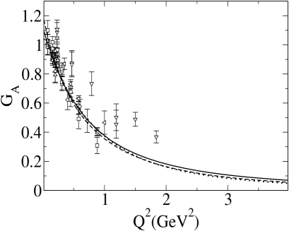
Figure 1: Axial form factor of the nucleon. Solid, dotted and dashed lines correspond to the instant, point and front forms respectively (from bruno02 ).

IV.2 The $\Delta(1232)\rightarrow N$ axial transition form factor

The calculated values for the $\Delta(1232)\rightarrow N$ transition form factor are shown in Fig. 2. The only empirical information on this form factor is that obtained by neutrino-induced reactions on the deuteron in Ref. Kitagaki . The value for $G_{A}^{\Delta}(0)$ extracted from this experiment is $G_{A}^{\Delta}(0)/\sqrt{2}=2.4\pm 0.25$ Hemmert . The present values for $G_{A}^{\Delta}(-m_{\pi}^{2})$ that are obtained in instant, point and front form kinematics are $G_{A}^{\Delta}(-m_{\pi}^{2})=1.74$, $G_{A}^{\Delta}(-m_{\pi}^{2})=1.70$ and $G_{A}^{\Delta}(-m_{\pi}^{2})=1.79$ thus clearly too small and also smaller than the semirelativistic quark model value 2.12 obtained in Ref. Hemmert .

For comparison the static quark model value for $G_{A}^{\Delta}(-m_{\pi}^{2})$ is $2\sqrt{2}$. It is worth noting than the experimental value for $G_{A}^{\Delta}(-m_{\pi}^{2})$ leads to a value for the pion decay constant which is too small by 30 %.

The results obtained are consistent with the assumption of quark-antiquark components in addition to the three-quark structure of the $\Delta(1232)$, which is supported by the observation that the ratios of the experimental pionic decay widths of $\Delta\to N\pi$, $\Sigma^{*}\to\Sigma\pi$, and $\Xi^{*}\to\Xi\pi$ do not follow the simple 3-quark expectation $9:4:1$ but are $12:4:1$, $\Delta(1232)$  riska03 .

In instant and front form $G_{A}^{\Delta}$ has very similar dependence on momentum transfer as the calculated corresponding elastic axial form factor of the nucleon. In contrast the calculated $G_{A}^{\Delta}$ in point form falls at a considerably slower rate than the corresponding elastic axial form factor of the nucleon.

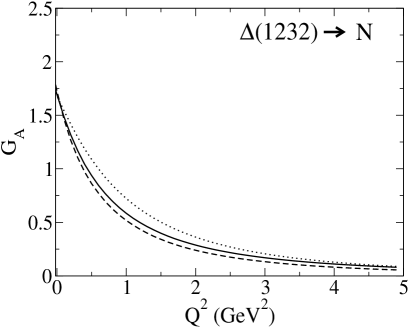
Figure 2: Axial form factor for the $N\to\Delta(1232)$ transition. Solid, dotted and dashed lines correspond to the instant, point and front forms respectively.

IV.3 The $N(1440)\rightarrow N$ axial transition form factor

The calculated $N(1440)\rightarrow N$ axial transition form factors are shown in Fig. 3. The form factors are qualitatively similar in the three forms, in all cases they change sign near $Q^{2}=0$. In instant and front form kinematics the sign change takes place in the timelike region ($Q^{2}<0$). The calculated values at the pion point are in all forms of kinematics smaller by a factor $\sim$ 4 than the corresponding values extracted from experiment that are shown in Table 2.

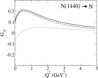
Figure 3: Axial form factor of the $N(1440)\to N$ transition. Solid, dotted and dashed lines correspond to the instant, point and front forms respectively.

IV.4 The $N(1535)\rightarrow N$ axial transition form factor

In Fig. 4 the $N(1535)\rightarrow N$ axial transition form factor is shown. The detailed evaluation is given in Appendix B. The $Q^{2}$ behavior of the form factor with the three forms is similar above $Q^{2}>2$ GeV², however the value at the pion point, $G_{A}^{N(1535)}(-m_{\pi}^{2})$, differs between the forms. All forms of kinematics give values that are close to the range of the values extracted from experiment (Table 2).

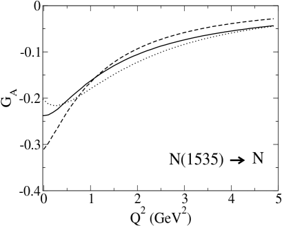
Figure 4: Axial form factor for $N\to N(1535)$ transition. Solid, dotted and dashed lines correspond to the instant, point and front forms respectively.

IV.5 The $\Delta(1600)\rightarrow N$ axial transition form factor

The axial form factors calculated with different kinematic currents are shown in Fig. 5. The differences are similar to those found for the $N(1440)\to N$ transition although the difference between instant and point form are more pronounced. At the pion point point form kinematics yields an unrealistically small value, (Table 2).

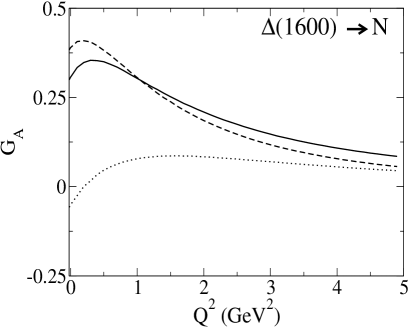
Figure 5: Axial form factor for the nucleon to Delta(1600) transition. Solid, dotted and dashed lines correspond to the instant, point and front forms respectively.

IV.6 Pion Decay Widths

The value of the axial form factor at the pion point, $G_{A}(Q^{2}=-m_{\pi}^{2})$, is related through expressions (24), (25) and (26), to the pion decay width of the corresponding resonances.

The calculated values for the pion decay widths are listed in Table 3 along with the empirical ranges for those values. The results in this table reveal that none of the form of kinematics is able to get values commensurable with the empirical ones. Instant and front form provide a comparable picture of the decay widths of these baryon resonances, while point form fails more abruptly than the others, in particular in the case of positive parity resonances. This failure of the point form of kinematics to provide a plausible picture of the pion decay widths has already been reported in Ref. melde .

Table 2: Axial form factors at the pion point, $|G_{A}(-m_{\pi}^{2})|$. The PHEN column contains the corresponding axial coupling constants that have been obtained phenomenologically from the imaginary parts of the corresponding resonance pole positions PDG using Eqs. (24) and (26).

	instant	point	front	PHEN
$\Delta(1232)$	1.74	1.70	1.79	2.67
$N(1440)$	0.11	0.07	0.10	[0.38$-$0.41]
$N(1535)$	0.24	0.20	0.31	[0.20$-$0.25]
$\Delta(1600)$	0.30	0.06	0.38	[0.48$-$0.75]

Table 3: Pion decay widths in MeV that correspond to 2 times the imaginary pole positions in PDG .

	instant	point	front	PHEN PDG
$\Delta(1232)$	42	41	45	100
$N(1440)$	10	4	8	[126$-$147]
$N(1535)$	84	60	147	[59$-$93]
$\Delta(1600)$	12	0	19	[30$-$75]

V Discussion

The results for the calculated axial transition form factors of the baryon resonances with the present simple representations show dependence on the kinematics used to generate the current operators. The spatial wave function was in each case parameterized so as to describe both the electromagnetic as well as the axial form factors of the nucleon (cf. Fig. 1). The results also exhibit a strong dependence on the representation of the excited states.

The calculated pion decay widths are in most cases considerably smaller than the empirically extracted values. This suggests that a description of the empirical values would call for sizable quark-antiquark components in the wave functions. Point form kinematics leads to unrealistically small values for the pion decay widths of the radial excitations of the nucleon and the $\Delta(1232)$ resonance. From the point of view of quark model phenomenology for the baryons the present results indicate a slight preference for front form kinematics over instant form kinematics.

Appendix A Boosts relating spin and spinor representations

Spin and spinor representations are related by appropriate representations of the Lorentz boosts $B(v)$. For spin ${\textstyle{1\over 2}}$ the spinor representation of canonical boosts $B_{c}(v)$ and null-plane boosts $B_{f}(v)$ are

$$S[B_{c}(v)] := D^{{\textstyle{1\over 2}},0}[B_{c}(v)]\oplus D^{0,{\textstyle{1\over 2}}}[B_{c}(v)]={\vec{\alpha}\cdot\vec{v}+1+v^{0}\over\sqrt{2(1+v^{0})}}$$ (46)

$$S[B_{f}(v)] := D^{{\textstyle{1\over 2}},0}[B_{f}(v)]\oplus D^{0,{\textstyle{1\over 2}}}[B_{f}(v)]={\alpha_{\perp}\cdot v_{\perp}+v^{+}\over\sqrt{v^{+}}}{1+\alpha_{z}\over 2}+{1\over\sqrt{v^{+}}}{1-\alpha_{z}\over 2}\,.$$ (47)

The spinor amplitudes $u_{c}(v)$ and $u_{f}(v)$ are defined by the boosts applied to the projections $(1+\beta)/2$ onto positive intrinsic parity,

$$u_{c}(v):=S[B_{c}(v)]{1+\beta\over 2}\;,\qquad u_{f}(v):=S[B_{f}(v)]{1+\beta\over 2}\;.$$ (48)

For spin ${\rm{1}}$ the appropriate boost representations are $D{{\textstyle{1\over 2}},{\textstyle{1\over 2}}}[B(v)]$ and the projections are the projections onto 4-vectors with vanishing time components. It follows that the spin-${\rm{1}}$ spinor amplitudes are 4-vectors orthogonal to the velocity. With canonical boosts the result is

$$\epsilon_{\lambda}(p) := e_{\lambda}+{e_{\lambda}\cdot p\over m+\omega}\left[{p\over m}+n_{c}\right]\,,\qquad\lambda=0\pm 1$$ (49)

with $n_{c}:=\{1,0,0,0\}$ and

$$e_{\lambda}=-\lambda{\hat{e}_{x}+\lambda i\hat{e}_{y}\over\sqrt{2}}\qquad\lambda=\pm 1;\qquad e_{0}=\hat{e}_{z}\,.$$ (50)

With null-plane boosts the amplitudes are

$$\epsilon_{\lambda}(p) := e_{\lambda}-{e_{\lambda}\cdot p\over n\cdot p}n\,,\qquad\lambda=0\pm 1$$

$$\epsilon_{0}(p) = {m\over n\cdot p}\left[n-{(n\cdot p)p\over p^{2}}\right]\,,$$ (51)

where $n:=\{-1,0,0,1\}$. The Rarita-Schwinger vector-spinor amplitudes of spin ${\textstyle{3\over 2}}$ baryons in Eq. (5), are

$$u^{\mu}_{\sigma}(v)=\sum_{\lambda,\sigma^{\prime}}\epsilon_{\lambda}^{\mu}(v)u_{\sigma}(v)(1,{\textstyle{1\over 2}},\lambda,\sigma^{\prime}|{\textstyle{3\over 2}},\sigma)\,.$$ (52)

Appendix B $N(1535)\to N$ axial transition form factor

When evaluating the transition form factor, $N(1535)\to N$, regardless of the form of kinematics, the following matrix elements need to be evaluated:

$$\langle{p;{\textstyle{1\over 2}}}|\,{\cal X\,F\,S}\,|{N(1535);{\textstyle{1\over 2}}}\rangle = {1\over\sqrt{2}}\sum_{ms}\langle 1,{\textstyle{1\over 2}},m,s;{\textstyle{1\over 2}}{\textstyle{1\over 2}}\rangle\;\langle{p,{\textstyle{1\over 2}}}|\,{\cal X\,F\,S}\,|{N_{(1535)}^{ms}}\rangle\,,$$ (53)

where ${\cal X\,F\,S}$ is, in general, an operator that acts on spatial, flavor and spin degrees of freedom. The operator entering the actual evaluation is a Wigner or Melosh rotated axial current operator. Its flavor part is simply: ${\cal F}=\tau_{z}$. The flavor matrix elements can be evaluated leaving the spin and spatial matrix elements, which do depend on the form of kinematics. We can write the wave functions explicitly in terms of their spin, flavor (some flavor indexes have been omitted for clarity) and spatial components:

$$\langle{p,{\textstyle{1\over 2}}}|\,{\cal X\,F\,S}\,|{N_{(1535)}^{ms}}\rangle = [3]_{x}\,[3]_{FS,S}^{1/2}\,{\cal X\,F\,S}\,{1\over\sqrt{2}}\left([21]_{x,S}^{m}[21]_{FS,S}^{s}+[21]_{x,A}^{m}[21]_{FS,A}^{s}\right)$$

$$= \left([3]_{x}\,{\cal X}\,[21]_{x,S}^{m}\;[3]_{FS,S}^{1/2}\,{\cal F\,S}\,[21]_{FS,S}^{s}+[3]_{x}\,{\cal X}\,[21]_{x,A}^{m}\;[3]_{FS,S}^{1/2}\,{\cal F\,S}\,[21]_{FS,A}^{s}\right)$$

where the spin-flavor symmetric and mixed-symmetric wave functions are,

$$\chi_{\sigma,\tau}\equiv\left[3\right]_{FS,S}^{\sigma,\tau} = {1\over\sqrt{2}}\left([21]_{F,S}^{\tau}[21]_{S,S}^{\sigma}+[21]_{F,A}^{\tau}[21]_{S,A}^{\sigma}\right)\,,$$

$$\chi_{+,\sigma,\tau}\equiv\left[21\right]_{FS,S}^{\sigma,\tau} = {1\over\sqrt{2}}\left([21]_{F,S}^{\tau}[21]_{S,S}^{\sigma}-[21]_{F,A}^{\tau}[21]_{S,A}^{\sigma}\right)\,,$$

$$\chi_{-,\sigma,\tau}\equiv\left[21\right]_{FS,A}^{\sigma,\tau} = {1\over\sqrt{2}}\left([21]_{F,S}^{\tau}[21]_{S,A}^{\sigma}+[21]_{F,A}^{\tau}[21]_{S,S}^{\sigma}\right)\,.$$ (55)

with the usual,

$$[3]_{S(T),S}^{l_{z}} = \sum_{abcm}({\textstyle{1\over 2}},{\textstyle{1\over 2}},a,b|1,m)({\textstyle{1\over 2}},1,c,m|{\textstyle{3\over 2}},l_{z})\;|{{\textstyle{1\over 2}},a}\rangle|{{\textstyle{1\over 2}},b}\rangle|{{\textstyle{1\over 2}},c}\rangle\,,$$

$$\left[21\right]_{S(T),S}^{l_{z}} = \sum_{abcm}({\textstyle{1\over 2}},{\textstyle{1\over 2}},a,b|1,m)({\textstyle{1\over 2}},1,c,m|{\textstyle{1\over 2}},l_{z})\;|{{\textstyle{1\over 2}},a}\rangle|{{\textstyle{1\over 2}},b}\rangle|{{\textstyle{1\over 2}},c}\rangle\,,$$

$$\left[21\right]_{S(T),A}^{l_{z}} = \sum_{ab}({\textstyle{1\over 2}},{\textstyle{1\over 2}},a,b|0,0)\;|{{\textstyle{1\over 2}},a}\rangle|{{\textstyle{1\over 2}},b}\rangle|{{\textstyle{1\over 2}},l_{z}}\rangle\,.$$ (56)

The spin-flavor matrix elements can be split into flavor and spin parts. The only nonzero flavor matrix elements are: $[21]_{F,S}\,\tau_{z}\,[21]_{F,S}=-1/3$ and $[21]_{F,A}\,\tau_{z}\,[21]_{F,A}=1$. Then the mixed-symmetric to symmetric part of Eq. (B) reads:

$$[3]_{FS,S}^{1/2}\,{\cal F\,S}\,[21]_{FS,S}^{s} = {1\over\sqrt{2}}\left([21]_{F,S}[21]_{S,S}^{1/2}+[21]_{F,A}[21]_{S,A}^{1/2}\right)\,{\cal F\,S}\,{1\over\sqrt{2}}\left([21]_{F,S}[21]_{S,S}^{s}-[21]_{F,A}[21]_{S,A}^{s}\right)$$ (57)

$$= {1\over 2}\bigg{(}[21]_{F,S}\,{\cal F}\,[21]_{F,S}\,[21]_{S,S}^{1/2}\,{\cal S}\,[21]_{S,S}^{s}-[21]_{F,A}\,{\cal F}\,[21]_{F,A}\,[21]_{S,A}\,{\cal S}\,[21]_{S,A}^{s}\bigg{)}$$

$$= {1\over 2}\bigg{[}-{1\over 3}[21]_{S,S}^{1/2}\,{\cal S}\,[21]_{S,S}^{s}-[21]_{S,A}^{1/2}\,{\cal S}\,[21]_{S,A}^{s}\bigg{]}$$

while the mixed-antisymmetric to symmetric has the form,

$$[3]_{FS,S}^{1/2}\,{\cal F\,S}\,[21]_{FS,A}^{s} = {1\over\sqrt{2}}\left([21]_{F,S}[21]_{S,S}^{1/2}+[21]_{F,A}[21]_{S,A}^{1/2}\right)\,{\cal F\,S}\,{1\over\sqrt{2}}\left([21]_{F,S}[21]_{S,A}^{s}+[21]_{F,A}[21]_{S,S}^{s}\right)$$ (58)

$$= {1\over 2}\bigg{[}[21]_{F,S}\,{\cal F}\,[21]_{F,S}\;[21]_{S,S}^{1/2}\,{\cal S}\,[21]_{S,A}^{s}+[21]_{F,A}\,{\cal F}\,[21]_{F,A}\;[21]_{S,A}^{1/2}\,{\cal S}\,[21]_{S,S}^{s}\bigg{]}$$

$$= {1\over 2}\bigg{[}-{1\over 3}[21]_{S,S}^{1/2}\,{\cal S}\,[21]_{S,A}^{s}+[21]_{S,A}^{1/2}\,{\cal S}\,[21]_{S,S}^{s}\bigg{]}\,.$$

giving

$$\langle{p,S}|\,{\cal X\,F\,S}\,|{N_{(1535)}^{ms}}\rangle = {1\over 2\sqrt{2}}\bigg{(}[3]_{x}\,{\cal X}\,[21]_{x,S}^{m}\;\bigg{[}-{1\over 3}[21]_{S,S}^{1/2}\,{\cal S}\,[21]_{S,S}^{s}-[21]_{S,A}^{1/2}\,{\cal S}\,[21]_{S,A}^{s}\bigg{]}$$ (59)

$$+[3]_{x}\,{\cal X}\,[21]_{x,A}^{m}\;\bigg{[}-{1\over 3}[21]_{S,S}^{1/2}\,{\cal S}\,[21]_{S,A}^{s}+[21]_{S,A}^{1/2}\,{\cal S}\,[21]_{S,S}^{s}\bigg{]}\bigg{)}\,,$$

and our initial matrix element reads:

$$\langle{p;{\textstyle{1\over 2}}}|\,{\cal X\,Q\,S}\,|{N(1535),{\textstyle{1\over 2}}}\rangle = \sum_{ms}\langle 1,{\textstyle{1\over 2}},m,s;{\textstyle{1\over 2}}{\textstyle{1\over 2}}\rangle{1\over 2\sqrt{2}}$$

$$\bigg{(}[3]_{x}\,{\cal X}\,[21]_{x,S}^{m}\;\bigg{[}-{1\over 3}[21]_{S,S}^{1/2}\,{\cal S}\,[21]_{S,S}^{s}-[21]_{S,A}^{1/2}\,{\cal S}\,[21]_{S,A}^{s}\bigg{]}$$

$$+[3]_{x}\,{\cal X}\,[21]_{x,A}^{m}\;\bigg{[}-{1\over 3}[21]_{S,S}^{1/2}\,{\cal S}\,[21]_{S,A}^{s}+[21]_{S,A}^{1/2}\,{\cal S}\,[21]_{S,S}^{s}\bigg{]}\bigg{)}\,.$$

The remaining matrix elements involve integrals over the spatial wave functions, $[3]_{x}\,{\cal X}\,[21]_{x,S}^{m}$ and $[3]_{x}\,{\cal X}\,[21]_{x,A}^{m}$, together with matrix elements involving the spins, $[21]_{S,A}\,{\cal S}\,[21]_{S,A}^{s}$ and $[21]_{S,A}\,{\cal S}\,[21]_{S,S}^{s}$, which are different for the different forms of kinematics.

The spin matrix elements correspond to matrix elements of the Wigner or Melosh rotated current,

$$[21]_{S,A}^{1/2}\,{\cal S}\,[21]_{S,A}^{s} = 3\;[21]_{S,A}\,\bigg{[}D^{1/2\dagger}_{2}D^{1/2}_{2}\bigg{]}\;\bigg{[}D^{1/2\dagger}_{3}D^{1/2}_{3}\bigg{]}\;\bigg{[}D^{1/2\dagger}_{1}I_{0q}D^{1/2}_{1}\bigg{]}\,[21]_{S,A}^{s}$$ (61)

and

$$[21]_{S,A}^{1/2}\,{\cal S}\,[21]_{S,S}^{s} = 3\;[21]_{S,A}\,\bigg{[}D^{1/2\dagger}_{2}D^{1/2}_{2}\bigg{]}\;\bigg{[}D^{1/2\dagger}_{3}D^{1/2}_{3}\bigg{]}\;\bigg{[}D^{1/2\dagger}_{1}I_{0q}D^{1/2}_{1}\bigg{]}\,[21]_{S,S}^{s}\,,$$ (62)

where $D^{1/2}$ are the representations of the corresponding Wigner or Melosh rotations for canonical and null-plane spins respectively.

References

- (1) F. Cano et al., Z. Phys. A 359, 315 (1997).
- (2) S. Capstick and W. Roberts, Prog. Part. Nucl. Phys. , S241 (2000).
- (3) L. Theussl et al., Eur. Phys. J. A12, 91 (2001).
- (4) T. R. Hemmert, B. R. Holstein and N. C. Mukhopadhyay, Phys. Rev. D 51, 158 (1995).
- (5) T. Sato and T.-S. H. Lee, Phys. Rev. C 63, 055201 (2001); T. Sato, D. Uno and T.-S. H. Lee, Phys. Rev. C 67, 065201 (2003).
- (6) B. Juliá-Díaz, D. O. Riska and F. Coester, Phys. Rev. C 69, 035212 (2004).
- (7) F. Coester, K. Dannbom, and D.O. Riska, Nucl. Phys. A 634, 335 (1998).
- (8) W. K. Cheng and C. W. Kim, Phys. Rev. 154, 1525 (1967).
- (9) P. L. Chung and F. Coester, Phys. Rev. D44, 229 (1991).
- (10) F. Coester, Progress on Nuclear and Particle Physics, 29, 1 (1992).
- (11) A. Del Guerra et al., Nucl. Phys. B 99, 253 (1975); P. Brauel et al., Phys. Lett. B 45, 389 (1973); E. Amaldi et al., Phys. Lett. B 41, 216 (1972); P. Joos et al., Phys. Lett. B 62, 230 (1976); E. D. Bloom et al., Phys. Rev. Lett. 30, 1186 (1973).
- (12) T. Kitagaki et al., Phys. Rev. D 42, 1331 (1990).
- (13) D. O. Riska, Eur. Phys. J. A 17, 297 (2003).
- (14) T. Melde, R. F. Wagenbrunn and W. Plessas, Few Body Syst. Suppl. 14, 37 (2003).
- (15) K. Hagiwara et al., Phys. Rev. D 66, 010001 (2002).