Determination of S₁₇(0) from published data

Abstract

The experimental landscape for the ⁷Be$+p$ radiative capture reaction is rapidly changing as new high precision data become available. We present an evaluation of existing data, detailing the treatment of systematic errors and discrepancies, and show how they constrain the astrophysical $S$ factor ($S_{17}$), independent of any nuclear structure model. With theoretical models robustly determining the behavior of the sub-threshold pole, the extrapolation error can be reduced and a constraint placed on the slope of $S_{17}$. Using only radiative capture data, we find $S_{17}(0)=20.7\pm 0.6(stat)\pm 1.0(syst)$ eV b if data sets are completely independent, while if data sets are completely correlated we find $S_{17}(0)=21.4\pm 0.5(stat)\pm 1.4(syst)$ eV b. The truth likely lies somewhere in between these two limits. Although we employ a formalism capable of treating discrepant data, we note that the central value of the $S$ factor is dominated by the recent high precision data of Junghans et al., which imply a substantially higher value than other radiative capture and indirect measurements. Therefore we conclude that further progress will require new high precision data with a detailed error budget.

I Introduction

The comparison of measured and predicted ⁸B solar neutrino fluxes represents a test of solar models and an opportunity to learn about the properties of the electron neutrinos produced in the Sun. Recent measurements at SNO SNO Collaboration (2004) have determined the total flux of active neutrinos emitted in the $\beta^{+}$ decay of ⁸B with a combined statistical and systematic precision of 9%. The implications of solar and reactor neutrino flux measurements for neutrino mixing parameters are explored in, e.g., Maltoni et al. (2003); Bandyopadhyay et al. (2004). Theoretical predictions of the ⁸B solar neutrino flux are now substantially more uncertain than the experimental measurements. Recent predictions have uncertainties of 20% Watanabe and Shibahashi (2001) and 15% Couvidat et al. (2003). The latest effort to estimate the theoretical uncertainty found a value of 23% Bahcall and Pinsonneault (2004). This error is completely dominated by the uncertainty in the heavy element abundance of the Sun, which has recently been revised to a level 2.5 times larger than the previous adopted value Bahcall et al. (2001). The contribution to the theoretical error budget made by S₁₇ has now been estimated at 3.6% based on the recommendation of S₁₇(0) = 21.4 $\pm$ 0.5 (expt.) $\pm$ 0.6 (theor.) eV b given in Junghans et al. (2003). Even if the uncertainty due to S₁₇ represents a small fraction of the total theoretical uncertainty, in our view an independent determination of its value based on the available experimental data and theoretical models is worthwhile. Here we provide reliable determinations of the total uncertainty in the $S$ factor, and find that nearly all previous analyses have underestimated the error.

In this paper we detail our fitting procedure, presenting formalisms for propagating systematic errors and combining multiple data sets, some of which were first presented in Cyburt (2004). We then describe the available data relevant for ⁷Be(p,$\gamma$)⁸B, and present the data sets used in this analysis. Next we briefly discuss the structure models used to extrapolate experimental data to solar energies, and the question of how the models can be tested. Finally, we present our constraints on the astrophysical $S$ factor using: (1) the energy dependence of the best structure models, (2) a pole model parametrization independent of structure models, and (3) a constrained pole model parametrization, where theory is used to robustly determine the behavior of the subthreshold pole.

II Fitting Procedure

It is often desirable to determine an average or best-fit representation of experimental data, and the uncertainties in such a representation. The standard techniques are generally not discussed in the literature, and are assumed to be well known. We detail here a formalism needed to properly take into account correlated data and systematic errors.

When modeling data, one generally uses a maximum likelihood or minimum $\chi^{2}$ formalism to determine the best fit. The $\chi^{2}$ is usually defined as:

$$\chi^{2}=\sum_{i}\left(\frac{y(x_{i})-\mu_{i}}{\sigma_{i}}\right)^{2},$$ (1)

where $\mu_{i}$, and $\sigma_{i}$ are the mean and standard deviation of the $i^{th}$ data point and $y(x)$ is the value calculated from the model we are using to describe the data as a function of the independent variable $x$ (e.g. $y(x)\rightarrow S_{17}(E)$). As an example, a linear model consists of $P$ parameters and $P$ basis functions (i.e. $y(x)=\sum_{p=1}^{P}a_{p}{\rm Y}_{p}(x)$). Minimizing $\chi^{2}$ defined in this way also minimizes the variance in the best fit model, but is limited in that it assumes the data points are independent and there is no explicit prescription for dealing with systematic errors or multiple data sets. A more general treatment has been described recently in an analysis of reaction cross sections relevant for big bang nucleosynthesis Cyburt (2004). We shall adopt a similar procedure for studying the ${}^{7}{\rm Be}({\rm p},\gamma)^{8}{\rm B}$ reaction. A clear understanding of how statistical and systematic uncertainties propagate through the analysis is an essential aspect of this approach. It is assumed that the dominant systematic error is the normalization uncertainty, which can be parametrized by a relative uncertainty, $\epsilon_{n}$, for each data set $n$. This global normalization error induces correlations between data points in the same data set. The correlation between two data points is given by Cyburt (2004):

$$C_{i_{n},j_{n}}=(1+\epsilon_{n}^{2})\sigma_{i_{n}}^{2}\delta_{i_{n},j_{n}}+\epsilon_{n}^{2}\mu_{i_{n}}\mu_{j_{n}},$$ (2)

where $\sigma_{i_{n}}$ is now the statistical uncertainty of the $i^{th}$ data point of data set n and $\delta_{i_{n},j_{n}}$ is the Kronecker delta. Using this correlation matrix, one can define a more general $\chi^{2}$:

$$\chi^{2}=\sum_{i,j}C_{i,j}^{-1}[y(x_{i})-\mu_{i}][y(x_{j})-\mu_{j}],$$ (3)

where we have left off the data set subscript $n$ for clarity. Given the simple form of the covariance matrix in Eq. 2, the inverse can be found analytically Cyburt (2004), and we obtain

$$C_{i,j}^{-1}=\frac{\delta_{i,j}}{(1+\epsilon^{2})\sigma_{i}^{2}}-\frac{\frac{\epsilon^{2}\mu_{i}\mu_{j}}{(1+\epsilon^{2})^{2}\sigma_{i}^{2}\sigma_{j}^{2}}}{1+\frac{\epsilon^{2}}{(1+\epsilon^{2})}\sum_{k}\left(\frac{\mu_{k}}{\sigma_{k}}\right)^{2}},$$ (4)

where we have again suppressed the index $n$. When the systematic errors are smaller than the statistical errors ($\epsilon_{n}\mu_{i_{n}}<\sigma_{i_{n}}$) or in the limit of large data sets, the $\chi^{2}$ of Eq. 3 reduces to that of Eq. 1, with the statistical error weighting the $\chi^{2}$ rather than the total error.

We stress that the $\chi^{2}$ quantity is a statistical device only; its minimum value tells us only how good the fit is within statistical uncertainties and its curvature tells us only about the statistical uncertainties in the fit. This is seen as a $1/\sqrt{N}$ scaling in the best fit uncertainty, where $N$ is the number of data points. Systematic errors are not reduced by this factor. The total uncertainty then consists of the statistical error and the intrinsic normalization error. Statistical errors contain no information about the quality of the fit. This can be seen by arbitrarily shifting data points away from each other, keeping their absolute uncertainties the same. We need an additional measure of how far data fall from the best fit. How then do we address the quality of the fit?

In Ref. Cyburt (2004), such a discrepancy error is defined as a measure of the fit quality. The discrepancy error is the weighted dispersion of the data relative to the best fit:

$$\epsilon_{disc}^{2}=\frac{\sum_{i,j}{\mathcal{C}}_{i,j}^{-1}[y(x_{i})-\mu_{i}][y(x_{j})-\mu_{j}]}{\sum_{i,j}{\mathcal{C}}_{i,j}^{-1}y(x_{i})y(x_{j})}.$$ (5)

The absolute size of this discrepancy error tells us how well the data are described by the best fit, while its size relative to the intrinsic normalization error quantifies possible unknown systematics. One may be tempted to reduce the size of the discrepancy error by the number of degrees of freedom (e.g. $\chi^{2}\rightarrow\chi^{2}/\nu$), but this is inappropriate because it assumes that the unknown errors we are trying to take into account can be propagated through the data analysis. As discussed earlier, systematics are not reduced by $1/\sqrt{N}$ as are statistical errors. We adopt a total normalization error defined as the quadrature sum of the intrinsic normalization error and this discrepancy error, as was done in Ref. Cyburt (2004).

We summarize our procedure for analyzing single data sets as follows.

1. We find best fits and statistical uncertainties, where the statistical errors of the data points dominate the $\chi^{2}$ analysis.

2. The total normalization error is the quadratic sum of the intrinsic normalization error and our quality-of-fit measure, the discrepancy error.

We are then left with the remaining question of how to treat multiple data sets. We discuss two methods. The first method, adopted in Cyburt (2004) treats the data sets as totally correlated and comprising a single data set. The second method treats the data sets as if they were completely independent. Reality is likely between these two possibilities; however at present we have no good prescription for determining how correlated data sets actually are, and therefore present results for these two limiting cases. Additionally, both methods yield similar results, suggesting that the methods are accurate and robust. Generally, the totally correlated method yields more conservative uncertainties as the intrinsic normalizations are not treated statistically.

II.1 Completely Correlated Data Sets

Assuming that individual data sets are totally correlated simplifies the analysis. Since the exact nature of the correlation is unknown, we cannot rigorously define a correlation matrix, so we continue to use the definition in Eq. 2 ($C_{i_{n},j_{m}}=\delta_{n,m}C_{i_{n},j_{n}}$) and its inverse in Eq. 4 ($C_{i_{n},j_{m}}^{-1}=\delta_{n,m}C_{i_{n},j_{n}}^{-1}$), generalized for multiple data sets. By virtue of the large data set limit for the inverse covariance matrix, we are led to the conclusion that the precise nature of the correlations is relatively unimportant, as the statistical uncertainties dominate the $\chi^{2}$ analysis.

As before, the total normalization error is the quadratic sum of the intrinsic normalization error and the discrepancy error ($\epsilon_{tot}^{2}=\epsilon_{norm}^{2}+\epsilon_{disc}^{2}$). The discrepancy error as defined in Eq. 5 is valid for a single data set and hence also for the case of totally correlated data sets. Since the individual data sets are completely correlated, the overall normalization error must be some average of the individual normalization errors. We adopt the normalization error prescription of Ref. Cyburt (2004):

$$\epsilon_{norm}^{2}=\frac{\sum_{n}\frac{\epsilon_{n}^{2}}{\chi^{2}_{n}}}{\sum_{n}\frac{1}{\chi^{2}_{n}}},$$ (6)

where $\epsilon_{n}$ are the individual data set normalization errors, and $\chi^{2}_{n}$ is the $\chi^{2}$ per datum of data set $n$ with respect to the best fit. This weighting scheme gives more weight to data sets that agree with the best fit model. We also point out that this normalization error assignment is bounded by the smallest and largest normalization errors and is not reduced by the number of data sets. This reflects the fact that the data sets are completely correlated and the normalization errors cannot be treated statistically in this case.

The expectation value and statistical variance of the best fit model are denoted $E[y(x)]$ and $V_{S}[y(x)]$, respectively. Including the normalization error, the total variance in the best fit model is $V_{T}[y(x)]=(1+\epsilon_{tot}^{2})V_{S}[y(x)]+\epsilon_{tot}^{2}E[y(x)]^{2}$. This completes our description of the formalism for completely correlated data sets, which we refer to as the correlated normalization analysis.

II.2 Completely Independent Data Sets

If data sets are truly independent from each other, we can treat the normalizations statistically, once best fits and statistical errors are found for each data set. We consider only linear models, for which $y(x)=\sum_{p=1}^{P}a_{p}{\rm Y}_{p}(x)$, where the ${\rm Y}_{p}(x)$ are known functions, and follow the prescription laid out in the previous section for each data set. The expectation value and statistical variance of $y(x)$ are $E[y(x)]=\sum_{p=1}^{P}\hat{a}_{p}{\rm Y}_{p}(x)$ and $V_{S}[y(x)]=\sum_{p,q=1}^{P}{\mathcal{C}}_{p,q}{\rm Y}_{p}(x){\rm Y}_{q}(x)$, respectively. With the best fit parameters $\hat{a}_{p}^{(n)}$ and parameter covariance ${\mathcal{C}}_{p,q}^{(n)}$ for each data set $n$ in hand, we can combine individual data sets and find a global best fit. Upon minimization, the $\chi^{2}$ can be decomposed as:

$$\chi^{2}=\chi^{2}_{min}+\sum_{n}\sum_{p,q=1}^{P}{{\mathcal{C}}_{p,q}^{(n)}}^{-1}(a_{p}-\hat{a}_{p}^{(n)})(a_{q}-\hat{a}_{q}^{(n)}),$$ (7)

where the calligraphic ${\mathcal{C}^{(n)}_{p,q}}$ is the covariance between the $p^{th}$ and $q^{th}$ parameters of the $n^{th}$ data set, with best fit parameters given by $\hat{a}_{p}^{(n)}$, provided there are at least as many data points $N$ as fitting parameters $P$. Note that with linear models all parameters are gaussian, i.e., the $\chi^{2}$ is a quadratic function of the parameters.

In order to combine multiple data sets, we must first replace the statistical variance, $V_{S}[y(x)]$, with the total variance $V_{T}[y(x)]$. In other words, we replace the parameter covariance matrix ${\mathcal{C}}_{p,q}^{(n)}$ for each data set $n$ with $(1+\epsilon_{tot,n}^{2}){\mathcal{C}}_{p,q}^{(n)}+\epsilon_{tot,n}^{2}\hat{a}_{p}^{(n)}\hat{a}_{q}^{(n)}$. Inserting this new parameter covariance into Eq. 7, we minimize the $\chi^{2}$ to find the best fit parameters and their statistical covariances, which now include the normalization errors of each data set.

We also need to quantify how well data sets agree with each other. The variance of the best global fit contains no information about the mutual consistency of data sets. This is seen if we shift the mean values of data points in a single data set, but keep the same absolute uncertainties. The parameter covariance is not changed, even though data sets can be severely discrepant. Thus we need to define a global discrepancy error. To do this, we calculate the renormalizations needed for the global best fit to minimize the $\chi^{2}$ for individual data sets. The dispersion of these renormalizations provides an estimate of the discrepancy between data sets. We find renormalizations $\alpha_{n}$ and their total errors $\sigma_{n}$ for each data set and then their dispersion according to

$$\epsilon_{disc}^{2}=\frac{\sum_{n}\left(\frac{\alpha_{n}-1}{\sigma_{n}}\right)^{2}}{\sum_{n}\frac{1}{\sigma_{n}^{2}}}.$$ (8)

This definition is similar to that discussed for the individual data sets, except that here no correlations exist between data sets. Given the global best fit $E[y(x)]$ and its statistical variance $V_{S}[y(x)]$, the total variance in this case is given by: $V_{T}[y(x)]=(1+\epsilon_{disc}^{2})V_{S}[y(x)]+\epsilon_{disc}^{2}E[y(x)]^{2}$. We refer to this formalism as the independent normalization analysis.

III The Data

With these formalisms in place, we now discuss the data available to constrain the astrophysical $S$ factor of the ⁷Be(p,$\gamma$)⁸B reaction. In some cases there is sufficient reason to exclude data sets from the analysis. We consider only low energy data, $E_{cm}<425$ keV, when determining the best fits to $S_{17}(E)$ as nuclear structure uncertainties complicate and render more uncertain the extrapolation when higher energy data are included Jennings et al. (1998); Davids and Typel (2003); Junghans et al. (2003).

III.1 Radiative Capture Data

Initially, we considered the data sets of Kavanagh Kavanagh (1960), Parker Parker (1966), Vaughn et al. Vaughn et al. (1970), Filippone et al. Filippone et al. (1983), Strieder et al. Strieder et al. (2001), Hammache-1 Hammache et al. (1998), Hammache-2 Hammache et al. (2001), Hass et al. Hass et al. (1999), Junghans-BE1 Junghans et al. (2002), Junghans-BE3 Junghans et al. (2003), and Baby et al. Baby et al. (2003). We exclude the data of Kavanagh Kavanagh (1960), Parker Parker (1966) and Vaughn et al. Vaughn et al. (1970) because these authors do not present enough information to adequately determine a normalization error. We do not use the measurement of Hass et al. Hass et al. (1999) simply because the data lie above our 425 keV energy cutoff.

Several details of our analysis bear mention here. One of the two target thickness determinations in the Filippone et al. measurement Filippone et al. (1983) relies on the ⁷Li(d,p) reaction. We adopt the recommendation of Adelberger et al. (1998) for the value of this reaction cross section. The Hammache-2 Hammache et al. (2001) data consist of 3 points, two of which are measured relative to the third. Ideally, one would like to include all 3 points, but not enough information is given on the third point to determine an intrinsic normalization error. We thus adopt the 2 relative measurements as the data set, using the third to determine the normalization error. Ref. Junghans et al. (2003) presents data from their BE1 measurement renormalized using the BE3 data. These renormalized BE1 data are not independent of the BE3 data. Therefore, we consider here the BE3 data Junghans et al. (2003) and the original BE1 data Junghans et al. (2002), which are independent. Finally we note that there is some discussion in the literature Junghans et al. (2003) regarding the uncertainties in the data of Baby et al. Baby et al. (2003). We take the uncertainties for this measurement from Table II of Ref. Baby et al. (2003).

III.2 Coulomb Dissociation Data

We considered the Coulomb dissociation (CD) data of Kikuchi et al. Kikuchi et al. (1997, 1998), Iwasa et al. Iwasa et al. (1999), Schümann et al. Schümann et al. (2003) and Davids et al. Davids et al. (2001); Davids and Typel (2003). We exclude the measurements of Kikuchi et al. Kikuchi et al. (1997, 1998) and Iwasa et al. Iwasa et al. (1999) due to concerns over the way these data were analyzed. The data from these measurements were not analyzed using a cut on the maximum scattering angle of the ⁸B center-of-mass, corresponding semiclassically to a minimum impact parameter. This means that the effects of nuclear absorption, diffraction dissociation, and $E2$ transitions are present in the data, and that the inferred $E1~{}S$ factors may not be reliable. Since we lack the detailed experimental information required to correct for these effects, we do not consider these data here. Hence we include only the CD data of Schümann et al. Schümann et al. (2003) and Davids et al. Davids et al. (2001); Davids and Typel (2003), which were analyzed using scattering angle cuts to minimize the nuclear and $E2$ contributions and their associated uncertainties.

IV Theoretical Structure Models

In general, two classes of models have been used to describe the structure of ⁸B, single particle potential models that treat ⁸B as a $p$-wave proton coupled to a ⁷Be core in its ground state, and microscopic cluster models that include two configurations of the three clusters ³He, $\alpha$, and a proton. Recently, most experimenters have used the cluster model of Descouvemont and Baye (DB) Descouvemont and Baye (1994) to extrapolate their data to zero energy. This generator coordinate method employs a central nucleon-nucleon interaction along with Coulomb and spin-orbit interactions. Ref. Descouvemont and Baye (1994) used the Volkov II nucleon-nucleon interaction Volkov (1965), while a more recent preliminary effort by Descouvemont and Dufour (DD) Descouvemont and Dufour (2004) opts for the Minnesota force Thompson et al. (1977), which describes low mass systems better. These cluster models include excited ⁷Be configurations. The single particle potential models generally employ a central Woods-Saxon + Coulomb potential, and optionally a spin-orbit interaction, which can be neglected in calculations of the $E1$ $S$ factor provided the central potential depth is properly adjusted. In these models, the $p$-wave potential depth is fixed by the ⁸B binding energy. The depths for the other partial waves can be chosen identically, but a better choice is to fix them using the well-measured $s$-wave scattering lengths for channel spin 1 and 2 in the isospin mirror system ⁷Li + $n$ Koester et al. (1983). The scattering lengths in the ⁷Be + $p$ system have also been measured Angulo et al. (2003), but with much lower precision. The scattering lengths for the dominant $S$ = 2 channel are consistent between the isospin mirrors, but there is a 2.7$\sigma$ discrepancy in the value for the $S$ = 1 channel. This discrepancy is not understood at present, and deserves attention in the future. In this work, we consider the DD cluster model and the ⁷Li + $n$ potential model of Davids and Typel (DT) Davids and Typel (2003), which reproduces the ⁷Li + $n$ scattering lengths. These models well represent their respective classes.

Both of these models have virtues. The cluster model allows more configurations than does the potential model, and therefore might be expected to describe the physics better. On the other hand, the potential model is simple, and has been tuned to reproduce the elastic scattering data. Fig. 1 shows the shapes predicted by the potential and cluster models.

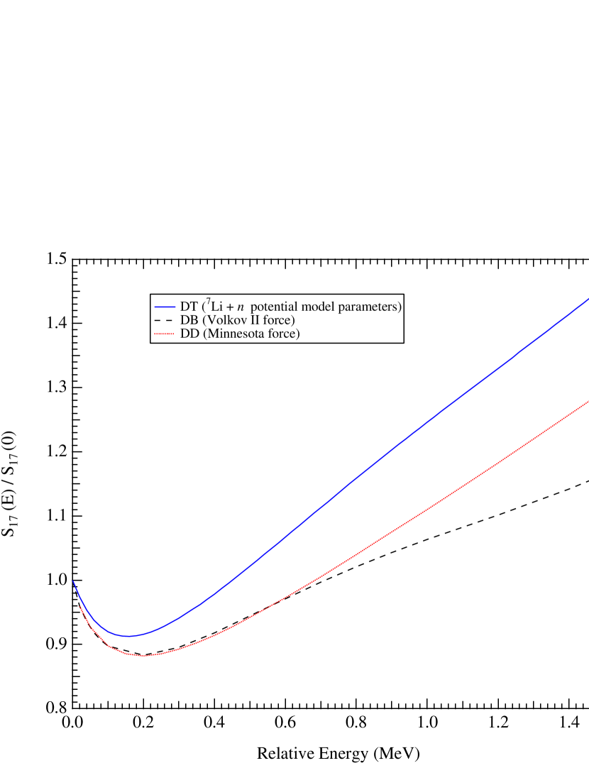
Figure 1: (Color online) Shapes of the $S$ factors predicted by the Descouvemont and Baye (DB) and Descouvemont and Dufour (DD) cluster models and the Davids and Typel (DT) potential model as a function of relative energy (E_cm). Shown is the ratio of the $E1$ $S$ factor to its value at E_cm = 0, which allows the shapes of models with different absolute normalizations to be shown in the same figure. The shapes of the two cluster models are very similar at low energies, but substantial deviations exist above 700 keV. The potential model is seen to have a slightly larger slope at high energies, but also a very different shape below 400 keV.

V Structure-Model-Dependent Analysis

With the theoretical structure models described briefly in Section IV, our fitting procedure involves only a single parameter, an absolute normalization. We fit data using the DT ⁷Li + $n$ potential model and the DD cluster model employing the formalism presented in Section II. Our results are summarized in Tables 1 and 2.

Table 1: Best fits to radiative capture (RC) and Coulomb dissociation (CD) data for $E_{cm}<425$ keV using the DT ⁷Li + $n$ potential model. Shown are the best fit astrophysical $S$ factors and their standard deviations (statistical) at $E_{cm}=0$. Also shown are the two individual contributions to the total systematic error, the intrinsic normalization error and the discrepancy error, given in percent. An additional potential model parameter uncertainty should be added to the other systematic errors, with $\epsilon_{model}$ = 0.01%, reflecting the small uncertainties in the ${}^{7}Li+n$ elastic scattering data.

	Data set (# of points)	$S_{17}(0)$ (eV b)	$\epsilon_{norm}$	$\epsilon_{disc}$
	Filippone (6)	$19.3\pm 0.5$	11.9%	5.6%
	Strieder (2)	$17.9\pm 0.6$	8.3%	2.7%
	Hammache-1 (3)	$19.4\pm 0.6$	4.9%	5.7%
Direct	Hammache-2 (2)	$18.8\pm 1.2$	12.2%	8.1%
	Junghans-BE1 (8)	$21.6\pm 0.2$	2.7%	0.7%
	Junghans-BE3 (13)	$21.2\pm 0.1$	2.3%	1.3%
	Baby (3)	$19.8\pm 0.7$	2.2%	2.2%
	Davids (2)	$16.6\pm 0.5$	7.1%	0.1%
CD	Schümann (2)	$18.4\pm 0.8$	5.6%	0.8%
	All RC but Junghans	$19.3\pm 0.7$	—	3.8%
indep.	Junghans	$21.4\pm 0.4$	—	0.8%
norm.	All radiative capture	$20.8\pm 0.4$	—	5.1%
	Coulomb dissociation	$17.5\pm 0.9$	—	5.5%
	All but Junghans	$19.1\pm 0.3$	8.5%	6.2%
corr.	Junghans	$21.3\pm 0.1$	2.6%	1.4%
norm.	All radiative capture	$21.2\pm 0.1$	5.6%	3.2%
	Coulomb dissociation	$17.1\pm 0.5$	6.7%	5.5%

Table 2: Same as table 1, except for the DD cluster model. A model uncertainty should be added to the other systematic errors, but DD do not present formal errors for this model.

	Data set	$S_{17}(0)$ (eV b)	$\epsilon_{norm}$	$\epsilon_{disc}$
	Filippone	$20.1\pm 0.5$	11.9%	6.1%
	Strieder	$18.8\pm 0.7$	8.3%	2.4%
	Hammache-1	$20.4\pm 0.7$	4.9%	5.9%
Direct	Hammache-2	$19.1\pm 1.2$	12.2%	8.2%
	Junghans-BE1	$22.6\pm 0.2$	2.7%	1.0%
	Junghans-BE3	$22.1\pm 0.1$	2.3%	1.4%
	Baby	$20.9\pm 0.7$	2.2%	2.7%
	Davids	$17.4\pm 0.6$	7.1%	1.0%
CD	Schümann	$19.2\pm 0.9$	5.6%	1.6%
	All RC but Junghans	$20.3\pm 0.7$	—	4.2%
indep.	Junghans	$22.3\pm 0.5$	—	1.1%
norm.	All radiative capture	$21.8\pm 0.4$	—	4.9%
	Coulomb dissociation	$18.2\pm 1.0$	—	5.3%
	All RC but Junghans	$20.0\pm 0.3$	8.6%	6.5%
corr.	Junghans	$22.2\pm 0.1$	2.5%	1.6%
norm.	All radiative capture	$22.1\pm 0.1$	5.5%	3.3%
	Coulomb dissociation	$17.9\pm 0.5$	6.7%	5.5%

We first derive best fits for individual experiments. The $S_{17}(0)$ determinations are in excellent agreement with previous analyses Junghans et al. (2003); Davids and Typel (2003). In general, the discrepancy errors are smaller than or comparable to the intrinsic normalization errors of each data set. Note that the central values of $S_{17}(0)$ for the radiative capture data range from 18-20 eV b and 21-22 eV b for non-Junghans and Junghans data sets respectively, while the CD data lie in the range of 16-19 eV b. This hints at some level of disagreement among the radiative capture data sets, especially when comparing the two Junghans experiments Junghans et al. (2002, 2003) with the other radiative capture data, in addition to that between the radiative capture and the CD data.

To further explore and quantify this disagreement we look at different combinations of the data in our multiple experiment fits. We first look at the radiative capture data alone. In these model-dependent analyses, we consider 3 combinations of the radiative capture data, (1) all but the Junghans data, (2) only Junghans data, and (3) all the radiative capture data. Using the DT ⁷Li + $n$ potential model, the independent normalization method gives for $S_{17}(0)$ in eV b: (1) $19.3\pm 1.0$, (2) $21.4\pm 0.5$ and (3) $20.8\pm 1.1$; using the correlated normalization method, we find (1) $19.1\pm 2.0$, (2) $21.3\pm 0.7$ and (3) $21.2\pm 1.4$ eV b. For the CD data we find $17.5\pm 1.3$ and $17.1\pm 1.6$ eV b using the independent normalization and correlated normalization methods respectively.

We find that the CD data and the non-Junghans radiative capture data are consistent, showing approximately a 1$\sigma$ discrepancy, while the CD data and Junghans data are discrepant at a little over the 2$\sigma$ level. Furthermore there is a 1 to 2$\sigma$ disagreement between the Junghans data and the other radiative capture measurements. The Junghans data dominate the fit when combining all the radiative capture data, due to their extremely small errors and the size of the data sets. Similar but somewhat higher results are obtained with the DD cluster model. Interestingly, the high precision Junghans data are described slightly better by the DT ⁷Li + $n$ potential model than by the DD cluster model, as seen in our quality-of-fit measure, the discrepancy error, but not at a significant level. The nature of the discrepancies between the Junghans data and both the non-Junghans radiative capture data and the CD data must be understood before we can address which model describes the data best. In an attempt to go beyond structure-model-dependent results, we now explore a structure-model-independent analysis.

VI Pole Model Analysis

Performing a structure-model-independent analysis will provide insight into the quality of existing data for the ⁷Be(p,$\gamma$)⁸B reaction below 425 keV. We use the expansion suggested by Jennings et al. (1998), adopting a three-parameter model:

$$S_{17}(E)=S_{17}(0)+\alpha\frac{E}{Q(E+Q)}+\beta E,$$ (9)

where $Q=137.5$ keV. In addition to terms constant and linear in energy, this functional form contains a simple pole term, a universal feature of radiative capture reactions that is independent of the details of nuclear structure models. We have chosen a fit that is linear in its parameters, but one can easily calculate the non-linear parameters adopted in Jennings et al. (1998): the pole term is given by $a=-\alpha/S_{17}(0)$ and the slope term by $c=\beta/S_{17}(0)$. A data set must have at least 3 data points in order for us to employ this three-parameter fit. Our results are summarized in Table 3. Of all the data, only the most recent Junghans-BE3 data set Junghans et al. (2003) provides a significant structure-model-independent constraint on the low energy behavior of the astrophysical $S$ factor, implying $S_{17}(0)=24.3\pm 4.0$ eV b. With this data set providing the only significant low-energy constraint on $S_{17}$, it dominates the fit when we combine the radiative capture data to find $23.6\pm 3.4$ eV b for the Junghans data and $23.4\pm 3.4$ eV b for all the radiative capture data, using the independent normalization method. Using the correlated normalization method we find $24.1\pm 3.4$ eV b for Junghans alone, and $18.9\pm 3.2$ eV b if we include all data sets. With the current data we can place robust constraints on the extrapolated value $S_{17}(0)$ independent of any particular structure model. We find that the central value is calculated to lie between 19-24 eV b with a total uncertainty of $\pm 3.5$ eV b.

Table 3: Best fit parameters for data with $E_{cm}<425$ keV with the pole model functional form of Eq. 9.

	Data	$S_{17}(0)$ (eV b)	$\alpha$ (eV b MeV)	$\beta$ (eV b MeV-1)	$\epsilon_{norm}$	$\epsilon_{disc}$
	Fillipone	$38.6\pm 15.7$	$-8.5\pm 5.4$	$70.6\pm 37.2$	11.9%	3.1%
	Hammache-1	$-2430\pm 2160$	$-623\pm 554$	$-2308\pm 2103$	4.9%	0.0%
RC	Junghans-BE1	$18.4\pm 10.6$	$-0.0\pm 3.2$	$7.1\pm 17.5$	2.7%	0.7%
	Junghans-BE3	$24.3\pm 3.9$	$-2.0\pm 1.3$	$18\pm 9$	2.3%	1.3%
	Baby	$55.3\pm 213.1$	$-11.4\pm 56.2$	$66\pm 229$	2.2%	0.0%
	All RC but Junghans	$34.9\pm 13.2$	$-7.2\pm 4.3$	$60.2\pm 27.4$	—	1.3%
indep.	Junghans	$23.6\pm 3.4$	$-1.7\pm 1.1$	$16.1\pm 7.1$	—	0.7%
norm.	All radiative capture	$23.4\pm 3.3$	$-1.8\pm 1.1$	$16.6\pm 6.8$	—	3.7%
	Coulomb dissociation	—	—	—	—	—
	All RC but Junghans	$35.4\pm 13.0$	$-7.1\pm 4.2$	$57.2\pm 26.8$	6.7%	3.6%
	All but Junghans	$29.0\pm 7.9$	$-5.0\pm 2.9$	$43.5\pm 21.2$	7.7%	5.4%
corr.	Junghans	$24.1\pm 3.4$	$-1.9\pm 1.1$	$18.5\pm 6.9$	2.6%	1.3%
norm.	All radiative capture	$18.9\pm 2.9$	$-0.1\pm 1.0$	$5.7\pm 6.1$	6.0%	3.2%
	Coulomb dissociation	$-13.5\pm 26.4$	$9.3\pm 8.6$	$-53\pm 53$	6.5%	3.6%

We see that in order to place a tighter constraint on $S_{17}$, one must assume some low-energy behavior. We now explore a constrained pole model which exploits knowledge of the astrophysical $S$ factor around its subthreshold pole, on which all theories agree.

VII Constrained Pole Model Analysis

In order to pin down the $S$ factor with higher precision, we need to examine the available theories and determine what, if any, universal information is available. To do this we fit each theory, normalized such that $S_{17}(0)\equiv 1$, using the pole model form, which now reduces to a 2 parameter fit, depending on the pole term $a=-\alpha/S_{17}(0)$ and the slope term $c=\beta/S_{17}(0)$. We fit to 4 theories, the two potential models of DT and the cluster-model calculations of DB and DD. Our results are summarized in Table 4.

Table 4: Best fit parameters for several theoretical structure models below $E_{cm}=425$ keV.

Model	$a$ (keV)	$c$ (MeV-1)
DT 7Li + $n$ potential	$45.7\pm 0.5$	$0.553\pm 0.007$
DT 7Be + $p$ potential	$45.0\pm 0.6$	$0.433\pm 0.007$
DB Volkov II	$45.5\pm 0.1$	$0.434\pm 0.001$
DD Minnesota	$44.5\pm 0.1$	$0.404\pm 0.002$

As one can see the pole term is robustly determined, with $a\in[44,46]$ keV. We adopt $a=45$ keV as our canonical value, and allow this information to propagate through our data analysis to see how our constraints on the low-energy behavior of $S_{17}$ improve. We thus use the two-parameter fit:

$$S_{17}(E)=S_{17}(0)\left[1-a\frac{E}{Q(E+Q)}\right]+\beta E,$$ (10)

with the parameter $a$ being fixed at 45 keV. Our results are summarized in Table 5.

Table 5: Results of a constrained pole model fit of radiative capture and Coulomb dissociation data below $E_{cm}=425$ keV. Shown are the best fit astrophysical $S$ factors, the associated slope parameter $\beta$, and their standard deviations (statistical). Also shown are both the intrinsic normalization errors and the discrepancy normalization errors for combined data sets, all cited in percent, which should be added in quadrature with the statistical errors to get the total error. An additional systematic error must be added due to the uncertainty in $a$; $\Delta S_{17}(0)/S_{17}(0)\approx 0.16\Delta a/a$, and $\Delta\beta/\beta\approx 0.80\Delta a/a$, which for $a=45\pm 1$ keV yields $\Delta S_{17}(0)/S_{17}(0)=0.4\%$ and $\Delta\beta/\beta=1.8\%$, respectively.

	Data set	$S_{17}(0)$ (eV b)	$\beta$ (eV b MeV-1)	$\epsilon_{norm}$	$\epsilon_{disc}$
	Filippone	$16.4\pm 2.8$	$18.1\pm 7.2$	11.9%	4.9%
	Strieder	$30.6\pm 17.2$	$-17.8\pm 37.6$	8.3%	4.0%
	Hammache-1	$-2.7\pm 16.7$	$56.2\pm 34.4$	4.9%	3.7%
RC	Hammache-2	$-2.3\pm 16.1$	$159.\pm 113.$	12.2%	0.0%
	Junghans-BE1	$21.4\pm 1.1$	$12.1\pm 2.6$	2.7%	0.7%
	Junghans-BE3	$21.4\pm 0.6$	$11.3\pm 1.6$	2.3%	1.3%
	Baby	$14.6\pm 8.5$	$21.9\pm 17.8$	2.2%	0.7%
	Davids	$16.6\pm 2.5$	$9.1\pm 6.4$	7.1%	0.0%
CD	Schümann	$17.5\pm 4.9$	$12.5\pm 13.2$	5.6%	0.0%
	All RC but Junghans	$16.3\pm 2.3$	$17.3\pm 5.0$	—	3.5%
indep.	Junghans	$21.4\pm 0.7$	$11.6\pm 1.4$	—	0.8%
norm.	All radiative capture	$20.7\pm 0.6$	$11.3\pm 1.3$	—	4.8%
	Coulomb dissociation	$17.5\pm 2.3$	$9.7\pm 5.8$	—	5.1%
	All RC but Junghans	$17.9\pm 1.4$	$13.4\pm 3.3$	8.0%	5.8%
corr.	Junghans	$21.1\pm 0.5$	$12.3\pm 1.3$	2.6%	1.3%
norm.	All radiative capture	$21.4\pm 0.5$	$11.0\pm 1.2$	5.7%	3.2%
	Coulomb dissociation	$17.4\pm 2.2$	$8.7\pm 5.7$	6.4%	4.8%

Using this information, individual experiments determine $S_{17}(0)$ much more precisely than in the unconstrained pole model fit. Again the Junghans data provide the strongest constraints, $21.4\pm 1.3$ eV b Junghans et al. (2002) and $21.4\pm 0.8$ eV b Junghans et al. (2003) respectively. However, the discrepancy between the two Junghans data sets and the other radiative capture experiments is quite apparent, with the fit to the combined Junghans data giving $21.4\pm 0.7$ eV b and the other radiative capture data yielding $16.3\pm 2.4$ eV b. This is a 2$\sigma$ discrepancy between these two low-energy extrapolations, using the independent normalization method. This tension is somewhat reduced in the correlated normalization method, which yields $21.1\pm 0.8$ eV b and $17.9\pm 2.3$ eV b for the Junghans and non-Junghans radiative capture data sets respectively, a discrepancy slightly more than 1$\sigma$. The CD data yield $17.5\pm 2.5$ eV b and $17.4\pm 2.6$ eV b using the independent normalization and correlated normalization methods, respectively. It is quite remarkable that the non-Junghans radiative capture data and the CD data agree so well, while both disagree with the Junghans data. This may be due to the sparseness of the data in these data sets, but the deviations from the Junghans results are significant. It would be desirable to have an independent confirmation of the Junghans measurements, since they deviate significantly from the other data and dominate the central value of combined fits.

At this time, it is unclear what is causing the discrepancies. Arguably, the Coulomb dissociation measurements have the least in common with the radiative capture measurements and large systematics of their own, so one could claim that they are the source of the discrepancy. However, this fails to explain the discrepancy among radiative capture measurements, namely between the two Junghans experiments Junghans et al. (2002, 2003) and that of Filippone Filippone et al. (1983), which dominates the non-Junghans data sets. As shown in Table 5, none of the other radiative capture measurements below $E_{cm}=425$ keV provides a significant constraint on $S_{17}(0)$. It is unclear which experiments are responsible for the discrepancy.

With these remaining uncertainties in mind, it is helpful to remind ourselves that we have defined a rigorous treatment for exactly these kinds of discrepancies. Our treatment has examined the level of concordance and quantified it in terms of a discrepancy error. We thus recommend an astrophysical $S$ factor at zero energy of:

$$S_{17}(0)=20.7\pm 1.2{\rm\ eV~{}b}\mbox{\ \ \rm indep. normalization}$$ (11)

$$S_{17}(0)=21.4\pm 1.4{\rm\ eV~{}b}\mbox{\ \ \rm corr. normalization}$$ (12)

for the radiative capture data, and

$$S_{17}(0)=17.5\pm 2.5{\rm\ eV~{}b}\mbox{\ \ \rm indep. normalization}$$ (13)

$$S_{17}(0)=17.4\pm 2.6{\rm\ eV~{}b}\mbox{\ \ \rm corr. normalization}$$ (14)

for the CD data.

One can compare our low-energy $S$ factor determinations with those determined from asymptotic normalization coefficients (ANCs). There are measurements from (1) proton transfer reactions Azhari et al. (2001), (2) ⁸B breakup reactions Trache et al. (2004) and (3) neutron transfer reactions Trache et al. (2003). The asymptotic normalization coefficient can be very simply related to the astrophysical $S$ factor, so we quote the measurements in these terms. These determinations yield (1) $17.3\pm 1.8$ eV b, (2) $18.7\pm 1.9$ eV b and (3) $17.6\pm 1.7$ eV b for the astrophysical $S$ factor of the ⁷Be(p,$\gamma$)⁸B reaction. These values of $S_{17}(0)$ agree perfectly with the CD data and non-Junghans radiative capture data. The ANC-derived $S$ factors disagree with the Junghans data at slightly more than the 1$\sigma$ level. Again, these discrepancies need to be more fully explored to better determine the low-energy behavior of the $S$ factor.

Thus far we have primarily discussed the low-energy extrapolations of the $S$ factor $S_{17}(0)$ and not the slope. Using our constrained pole model we find that the slopes based on the non-Junghans radiative capture, Junghans, and CD data are all roughly consistent with each other. In fact, the Junghans and CD slopes agree remarkable well, though the CD data have sizable errors. The non-Junghans radiative capture slope disagrees at the 1$\sigma$ level with both the Junghans and the CD data. Again, the non-Junghans fit is dominated by the Filippone Filippone et al. (1983) data, with substantial uncertainties. These discrepancies disappear when one uses the correlated normalization method, suggesting that no significant deviation in the slope is observed and that the constraint on the slope using $E_{cm}<425$ keV data is not particularly strong. The fact that the statistical errors in this parameter dominate over the normalization error supports this.

VIII Conclusions

We have presented a robust formalism for fitting data that both properly propagates known systematic uncertainties and quantifies the quality of fit, incorporating a discrepancy error into the total systematic error. We discuss two limiting cases, one in which data sets are considered completely independent from each other, and a second in which all data sets are totally correlated. These two methods, the independent normalization and correlated normalization methods, yield similar results, providing robust constraints and suggesting that most previous analyses have underestimated the true uncertainty.

A structure-model-dependent analysis was performed using the DT ⁷Li + $n$ potential Davids and Typel (2003) and the DD Minnesota force cluster Descouvemont and Dufour (2004) models. The ⁷Li + $n$ potential model generally predicts low-energy extrapolated $S$ factors smaller than the Minnesota-interaction cluster model. With the available data, no significant preference for one model is observed. We explored a structure-model-independent fit to the data, finding that only the Junghans Junghans et al. (2003) data placed even modest constraints on the low-energy $S$ factor. Identifying a feature common to all models, the relative strength of the subthreshold pole term, we reduced the extrapolation error considerably. Even though we find evidence for discrepancies between the Junghans et al. radiative capture measurements and the others Filippone et al. (1983); Strieder et al. (2001); Hammache et al. (2001, 1998); Baby et al. (2003)), our rigorous and careful treatment of systematic errors provides a robust determination of $S_{17}(0)$. Our analysis of indirect Coulomb dissociation data Schümann et al. (2003); Davids and Typel (2003) and ANC determinations Azhari et al. (2001); Trache et al. (2003, 2004) found mutual agreement and consistency with the radiative capture measurements other than those of Junghans et al.

The dominant source of error in the standard solar model predictions for the total ⁸B neutrino flux is the uncertainty in the heavy metal abundance. The dominant nuclear uncertainties stem from uncertainties in the ³He($\alpha$,$\gamma$)⁷Be and ⁷Be(p,$\gamma$)⁸B reactions. Using a technique similar to that employed here, the authors of Cyburt (2004) find a total error in the $S_{34}$ normalization of 17%. If we adopt our determination of $S_{17}(0)$ using the independent normalization method (Eq. 11) and the $S_{34}$ error assignment from Cyburt (2004) we find the following standard solar model (BP04) Bahcall and Pinsonneault (2004) prediction for the total ⁸B solar neutrino flux in units of $10^{6}$ cm^-2 s^-1:

$$\phi(^{8}{\rm B})=5.63\left[1\pm 0.058(S_{17})\pm 0.15(S_{34})\pm 0.21\right].$$ (15)

Here we have separated the individual contributions to the total error in the neutrino flux, those from $S_{17}$, $S_{34}$, and the other standard solar model parameters, which when added in quadrature yield a total error of 26%. We can see that the new $S_{17}$ error assignment contributes 6% to the total neutrino flux error.

While S₁₇ now makes only a relatively small contribution to the total uncertainty in the predicted ⁸B solar neutrino flux, ongoing measurements of S₃₄ and improved radiative opacity tables may reduce the other solar model uncertainties substantially in the near future. In order to further reduce the uncertainty on S₁₇, a new high precision measurement with a detailed error budget would be required.

IX Acknowledgements

This work was supported by the Natural Sciences and Engineering Research Council of Canada. We acknowledges helpful discussions with Shung-ichi Ando, Sam Austin, Carlo Barbieri, Michael Hass, Kurt Snover, Jean-Marc Sparenberg, Lukas Theussel, and Brian Fields.

References

- SNO Collaboration (2004) SNO Collaboration, Phys. Rev. Lett. 92, 181301 (2004), eprint nucl-ex/0309004.
- Maltoni et al. (2003) M. Maltoni, T. Schwetz, M. A. Tórtola, and J. W. Valle, Phys. Rev. D 68, 113010 (2003).
- Bandyopadhyay et al. (2004) A. Bandyopadhyay, S. Choubey, S. Goswami, S. T. Petcov, and D. P. Roy, Physics Letters B 583, 134 (2004).
- Watanabe and Shibahashi (2001) S. Watanabe and H. Shibahashi, Publ. Astron. Soc. Japan 53, 565 (2001).
- Couvidat et al. (2003) S. Couvidat, S. Turck-Chièze, and A. G. Kosovichev, Astrophys. J. 599, 1434 (2003).
- Bahcall and Pinsonneault (2004) J. N. Bahcall and M. H. Pinsonneault, Phys. Rev. Lett. 93, 121301 (2004), eprint astro-ph/0402114.
- Bahcall et al. (2001) J. N. Bahcall, M. H. Pinsonneault, and S. Basu, Astrophys. J. 555, 990 (2001).
- Junghans et al. (2003) A. R. Junghans, E. C. Mohrmann, K. A. Snover, T. D. Steiger, E. G. Adelberger, J. M. Casandjian, H. E. Swanson, L. Buchmann, S. H. Park, A. Zyuzin, et al., Phys. Rev. C 68, 065803 (2003).
- Cyburt (2004) R. H. Cyburt, Phys. Rev. D 70, 023505 (2004).
- Jennings et al. (1998) B. K. Jennings, S. Karataglidis, and T. D. Shoppa, Phys. Rev. C 58, 3711 (1998).
- Davids and Typel (2003) B. Davids and S. Typel, Phys. Rev. C 68, 045802 (2003).
- Kavanagh (1960) R. W. Kavanagh, Nuclear Physics 15, 411 (1960).
- Parker (1966) P. D. Parker, Physical Review 150, 851 (1966).
- Vaughn et al. (1970) F. J. Vaughn, R. A. Chalmers, D. Kohler, and L. F. J. Chase, Phys. Rev. C 2, 1657 (1970).
- Filippone et al. (1983) B. W. Filippone, A. J. Elwyn, C. N. Davids, and D. D. Koetke, Phys. Rev. C 28, 2222 (1983).
- Strieder et al. (2001) F. Strieder, L. Gialanella, G. Gyürky, F. Schümann, R. Bonetti, C. Broggini, L. Campajola, P. Corvisiero, H. Costantini, A. D’Onofrio, et al., Nucl. Phys. A 696, 219 (2001).
- Hammache et al. (1998) F. Hammache, G. Bogaert, P. Aguer, C. Angulo, S. Barhoumi, L. Brillard, J. F. Chemin, G. Claverie, A. Coc, M. Hussonnois, et al., Phys. Rev. Lett. 80, 928 (1998).
- Hammache et al. (2001) F. Hammache, G. Bogaert, P. Aguer, C. Angulo, S. Barhoumi, L. Brillard, J. F. Chemin, G. Claverie, A. Coc, M. Hussonnois, et al., Phys. Rev. Lett. 86, 3985 (2001).
- Hass et al. (1999) M. Hass, C. Broude, V. Fedoseev, G. Goldring, G. Huber, J. Lettry, V. Mishin, H. J. Ravn, V. Sebastian, and L. Weissman, Phys. Lett. B 462, 237 (1999).
- Junghans et al. (2002) A. R. Junghans, E. C. Mohrmann, K. A. Snover, T. D. Steiger, E. G. Adelberger, J. M. Casandjian, H. E. Swanson, L. Buchmann, S. H. Park, and A. Zyuzin, Phys. Rev. Lett. 88, 41101 (2002).
- Baby et al. (2003) L. T. Baby, C. Bordeanu, G. Goldring, M. Hass, L. Weissman, V. N. Fedoseyev, U. Köster, Y. Nir-El, G. Haquin, H. W. Gäggeler, et al., Phys. Rev. C 67, 65805 (2003).
- Adelberger et al. (1998) E. G. Adelberger, S. M. Austin, J. N. Bahcall, A. B. Balantekin, G. Bogaert, L. S. Brown, L. Buchmann, F. E. Cecil, A. E. Champagne, L. de Braeckeleer, et al., Rev. Mod. Phys. 70, 1265 (1998).
- Kikuchi et al. (1997) T. Kikuchi, T. Motobayashi, N. Iwasa, Y. Ando, M. Kurokawa, S. Moriya, H. Murakami, T. Nishio, J. Ruan (Gen), S. Shirato, et al., Phys. Lett. B 391, 261 (1997).
- Kikuchi et al. (1998) T. Kikuchi, T. Motobayashi, N. Iwasa, Y. Ando, M. Kurokawa, S. Moriya, H. Murakami, T. Nishio, J. Ruan, S. Shirato, et al., Eur. Phys. J. A 3, 213 (1998).
- Iwasa et al. (1999) N. Iwasa, F. Boué, G. Surówka, K. Sümmerer, T. Baumann, B. Blank, S. Czajkowski, A. Förster, M. Gai, H. Geissel, et al., Phys. Rev. Lett. 83, 2910 (1999).
- Schümann et al. (2003) F. Schümann, F. Hammache, S. Typel, F. Uhlig, K. Sümmerer, I. Böttcher, D. Cortina, A. Förster, M. Gai, H. Geissel, et al., Phys. Rev. Lett. 90, 232501 (2003).
- Davids et al. (2001) B. Davids, D. W. Anthony, T. Aumann, S. M. Austin, T. Baumann, D. Bazin, R. R. Clement, C. N. Davids, H. Esbensen, P. A. Lofy, et al., Phys. Rev. Lett. 86, 2750 (2001).
- Descouvemont and Baye (1994) P. Descouvemont and D. Baye, Nucl. Phys. A 567, 341 (1994).
- Volkov (1965) A. B. Volkov, Nuclear Physics 74, 33 (1965).
- Descouvemont and Dufour (2004) P. Descouvemont and M. Dufour, Nucl. Phys. A 738, 150 (2004).
- Thompson et al. (1977) D. R. Thompson, M. Lemere, and Y. C. Tang, Nuclear Physics A 286, 53 (1977).
- Koester et al. (1983) L. Koester, K. Knopf, and W. Waschkowski, Z. Phys. A 312, 81 (1983).
- Angulo et al. (2003) C. Angulo, M. Azzouz, P. Descouvemont, G. Tabacaru, D. Baye, M. Cogneau, M. Couder, T. Davinson, A. di Pietro, P. Figuera, et al., Nucl. Phys. A 716, 211 (2003).
- Azhari et al. (2001) A. Azhari, V. Burjan, F. Carstoiu, C. A. Gagliardi, V. Kroha, A. M. Mukhamedzhanov, F. M. Nunes, X. Tang, L. Trache, and R. E. Tribble, Phys. Rev. C 63, 55803 (2001).
- Trache et al. (2004) L. Trache, F. Carstoiu, C. A. Gagliardi, and R. E. Tribble, Phys. Rev. C 69, 032802 (2004).
- Trache et al. (2003) L. Trache, A. Azhari, F. Carstoiu, H. L. Clark, C. A. Gagliardi, Y.-W. Lui, A. M. Mukhamedzhanov, X. Tang, N. Timofeyuk, and R. E. Tribble, Phys. Rev. C 67, 62801 (2003).