Effective theories of scattering with an attractive inverse-square potential
and the three-body problem

Abstract

A distorted-wave version of the renormalisation group is applied to scattering by an inverse-square potential and to three-body systems. In attractive three-body systems, the short-distance wave function satisfies a Schrödinger equation with an attractive inverse-square potential, as shown by Efimov. The resulting oscillatory behaviour controls the renormalisation of the three-body interactions, with the renormalisation-group flow tending to a limit cycle as the cut-off is lowered. The approach used here leads to single-valued potentials with discontinuities as the bound states are cut off. The perturbations around the cycle start with a marginal term whose effect is simply to change the phase of the short-distance oscillations, or the self-adjoint extension of the singular Hamiltonian. The full power counting in terms of the energy and two-body scattering length is constructed for short-range three-body forces.

I Introduction

The successful application of effective field theories (EFT’s) to two-body scattering has revived interest in developing model-independent treatments of few-body systems, as reviewed in Refs. border ; bvkrev . In the case of two-body systems EFT’s provide a framework within which the old idea of the effective-range expansion bethe ; bj can be extended systematically to describe electromagnetic or weak couplings. Their application to three-body systems requires the addition of three-body forces. The observation that such forces are essential for describing low-energy three-body observables goes back to the work of Phillips phillips . One model-independent way of introducing them is the boundary-condition method developed by Brayshaw brayshaw . The EFT approach provides a more practical way of doing so, and one which can be extended to include couplings to external currents.

In the case of two-body scattering, these EFT’s have been well explored. If there is a clear separation between the low-energy scales of interest and the high-energy scales characterising the underlying physics, then the interactions terms in the effective Lagrangian can be organised systematically as an expansion in powers of ratios of low-energy to high-energy scales. For weakly interacting systems the power counting in this expansion is just that of naive dimensional analysis. Since this is the same as the counting in chiral perturbation theory wein79 ; wein , it is usually known as “Weinberg counting”.

In contrast, in strongly interacting systems with shallow resonances or bound states, simple dimensional analysis is no longer appropriate because of the appearance of new low-energy scales. These result in a need to resum certain terms wein ; uvk . This has been done within various frameworks uvk ; ksw ; bmr ; geg , all of which lead to the the same power counting. The resulting scheme is often referred to as “KSW counting”. For systems with short-range forces only, it is in fact equivalent to the effective-range expansion developed by Bethe and others bethe ; bj . This expansion is the relevant one for few-nucleon systems at low energies, where the deuteron and the ${}^{1}S_{0}$ virtual state lie very close to threshold. It may also apply to atomic systems where Feshbach resonances can be tuned to give large scattering lengths.

Both of these power-counting schemes can be understood using the Wilsonian renormalisation group (RG) wilson . Fixed points of the RG describe scale-free systems. The RG flow near these points can then be used to define a power counting for organising the perturbations around them. Weinberg counting arises from the expansion around the trivial fixed point of the RG, corresponding to a noninteracting system. KSW counting, or the effective-range expansion, is associated with a second, nontrivial fixed point corresponding to a system with a bound-state exactly at threshold.

The RG approach can also be extended to systems with known long-range interactions, such as the Coulomb or one-pion-exchange potentials, provided one has identified all the low-energy scales. In Ref. bb1 we applied this to examples including Coulomb and repulsive inverse-square potentials, for which well-defined distorted waves (DW’s) exist. We refer to this extended version as the distorted-wave RG (DWRG). In it, a cut-off is applied to the basis of DW’s of the known long-range potential so that that potential is unaffected by the cut-off. The advantage of the method is that it provides a clean separation between the short- and long-range physics. The resulting nontrivial fixed point corresponds to a DW or “modified” version of the effective-range expansion bethe ; vhk . In this paper, we use the DWRG to determine the power-counting for three-body forces. A very brief account of these ideas was previously presented in Ref. bb2 and a much more extensive one can be found in the Ph.D. thesis, Ref. tbthesis .

The EFT description of systems of three particles must include three-body forces, represented by six-point interactions in the Lagrangian. To develop a model-independent treatment of these systems, we use a two-body EFT with couplings fixed by two-body data, and augment it with three-body terms. However a consistent power counting needs to be determined for these new interactions.

Complications arise in three-body systems because there can be long-range forces resulting from the exchange of one of the three particles. The range of these forces is controlled by the two-body scattering lengths. In weakly interacting systems, where the size of the scattering lengths is determined by the scale of the underlying physics, these forces can be treated as short-range and Weinberg counting applies to the three-body interactions. On the other hand, systems with shallow bound or virtual states have large two-body scattering lengths and hence long-range forces. Hence for systems where the two-body forces can be organised with KSW counting, the correspnding power-counting for the three-body forces is difficult to determine.

Bedaque et al. bvk ; bhvk were the first to look at the problem of short-range three-body forces in EFT’s. Their method is based on the equation originally derived by Skorniakov and Ter-Martirosian (STM) stm for systems with zero-range two-body forces. In higher partial waves and in $s$-wave nuclear systems with spin or isospin $\frac{3}{2}$ they found that the three-body interactions are irrelevant (in the technical RG sense that they vanish as the cut-off is lowered). This is because centrifugal forces or the Pauli exclusion principle act to ensure that these systems are insensitive to short-range physics. In contrast, for three bosons in $s$-waves or three $s$-wave nucleons with total angular momentum and isospin $\frac{1}{2}$, there is nothing to prevent all three particles from coming together. Bedaque et al. found that three-body forces are not merely important in these systems, they are in fact essential for producing well-defined results bvk ; bhvk (see also Refs. bbh ; hm ). More recently, a power-counting scheme for the three-body forces in these systems has been constructed by renormalising the STM equation order-by-order in the energy bghr . Our work confirms this power counting within the framework of a full RG analysis.

In other recent work on this problem, Phillips and Afnan pa have looked at the STM equation in the case of three $s$-wave bosons. They were able to reproduce the results of Bedaque et al. by using a subtractive renormalisation and introducing a single piece of three-body data, namely the three-body scattering length. The introduction of this piece of data is equivalent to the LO three-body force of Ref. bhvk . Similar results have also been obtained by Mohr mohr .

An alternative to the STM equation for three-body systems with contact interations is provided by the work of Efimov efimov (for a review, see Ref. acp ). In general, Efimov’s equations are difficult to solve (see, for example, fedorov ) because they involve a nonseparable boundary condition. However, in the case of infinite two-body scattering length, the equations become separable in suitable cooordinates and can be solved exactly. In this limit the Hamiltonian becomes scale free, which should not be surprising given that this is the nontrivial fixed point of the two-body system. In hyperspherical coordinates, the corresponding three-body Hamiltonian contains an inverse-square potential (ISP).

The strength of the ISP is determined by the statistics of the system. In systems with nonzero orbital angular momentum or where the Pauli exclusion principle keeps the particles apart, the potential is repulsive. However if there is no angular momentum or exclusion principle, as for three $s$-wave bosons, there can be an attractive ISP. This corresponds to the cases where Bedaque et al. found a need for a three-body force.

Because of its relevance to three-body EFTs, the attractive ISP has been the subject of several recent papers bc ; co ; bp . It will also play a central role in this paper, since the DWRG analysis for scattering in the presence of this potential will also provide the basic power counting for the three-body system. The attractive ISP is particularly interesting from a mathematical point of view because it is sufficiently singular that its wave functions have a logarithmic oscillatory behaviour near the origin newton . This makes it impossible to define a “regular” boundary condition on the wavefunctions at the origin. Mathematically, the resolution of this quandary is well known: we need to form a self-adjoint extension of the Hamiltonian meetz ; case ; pp . More physically, one can think of this as introducing a boundary condition to fix the phase of the oscillatory solutions near the origin.

Although choosing a self-adjoint extension ensures that all observables are uniquely defined, it does not lead to a ground state. Instead the bound states form an infinite tower with geometrically spaced energies. This pattern was found by Efimov in the context of three-body systems efimov , although the lack of a ground state was noted first by Thomas thomas . The pattern is not quite scale-free since it requires the input of a new scale, such as the energy of one of the bound states. This scale is provided by the self-adjoint extension.

An alternative to introducing a boundary condition to fix the self-adjoint extension of the ISP is to regulate the singularity of the potential at short distances and introduce a counterterm beane ; bc . In essence this is what the momentum-space regularisation of the STM equation does for the three-body problem bhvk ; hm ; bghr . Again, one piece of three-body data is needed to fix the scale in the extension, as also noted by Phillips and Afnan pa . Other authors have shown explicitly how a short-range force can be used to select an extension bc ; beane ; bp , but have not developed the power counting for all possible terms in that force. Furthermore, the three-body forces obtained in this manner turn out to be multi-valued, with no obvious procedure to resolve this bc ; bp .

An interesting feature of the approaches based on regularisation of the singular interaction is that they exhibit a cyclic behaviour as the scale of the cut-off is varied bhvk ; hm ; beane ; bc . In fact, as pointed out by Wilson wilslc , they form a novel kind of limit cycle of the RG. Several examples of this have only recently been highlighted gw ; leclair ; mh . In addition, Braaten and Hammer have pointed out that a rather minor fine tuning of the quark masses in QCD would bring the infrared limit of the theory to the effective-range fixed point in the two-nucleon channel, and hence to a limit cycle for three nucleons bh .

In this paper we apply the DWRG method, first to the attractive ISP corresponding to three-body systems with infinite two-body scattering length, and then to more general attractive three-body systems. We apply a cut-off to the deeply bound states as well as the continuum, and this leads to an RG equation with single-valued but discontinuous solutions. As already mentioned, the results confirm the power counting found by Bedaque et al. bghr . By taking advantage of Efimov’s separation of the full three-body wave function, we are able to show that this power counting is not limited to the STM “slice” through it, where two of the particles coincide. Because of the clean separation of short- and long-range physics in the DWRG, we are able to derive this counting in a more transparent way.

The lowest-order three-body interaction is marginal, in the sense that its RG flow is only logarithmic in the cut-off. As we shall explicitly show, it represents the same degree of freedom as the choice of self-adjoint extension. The resulting three-body interaction is built out of perturbations around a single-valued limit-cycle solution of the DWRG. By constructing the corresponding physical scattering amplitudes, we are able to directly relate the coefficients in the three-body potential to observables, through a version of the DW effective-range expansion.

II The RG for three-body forces

For simplicity, we consider here a system of three bosons of mass $M$, in a state of zero orbital angular momentum. We assume that the two-body interaction produces a single shallow bound state with binding energy $\gamma^{2}/M$, corresponding to a “binding momentum” $i\gamma$. We start by considering the effects of two-body forces only and we denote the corresponding three-body Green’s function by $G_{2}(p)$, where $p$ is defined in terms of the total centre-of-mass energy by $E=p^{2}/M$. This function has the spectral decomposition,

$$G_{2}(p)=\frac{M}{4\pi}\sum_{n=1}^{N}\frac{|\Psi_{n}\rangle\langle\Psi_{n}|}{p^{2}+p_{n}^{2}}+\frac{M}{2\pi^{2}}\int_{-\gamma^{2}}^{\infty}d(q^{2})\frac{1}{p^{2}-q^{2}+i\epsilon}\left[|\Psi_{q,i\gamma}\rangle\langle\Psi_{q,i\gamma}|+\vartheta(q^{2})\frac{2}{\pi}\int_{0}^{q}dk\,|\Psi_{q,k}\rangle\langle\Psi_{q,k}|\right],$$ (1)

where $\vartheta(x)$ is the unit step function. Note that in a system with two-body contact interactions, we require an additional boundary condition to define the DW’s and hence the Green’s function, as discussed below.

Three types of wave appear in this decomposition. In the first term, we have the bound states of three particles, $|\Psi_{n}\rangle$. In the final term, we have states with three incoming free particles, $|\Psi_{q,k}\rangle$, which we label by their total centre-of-mass energy, $E=q^{2}/M$, and relative momentum, $k$. In the middle are states with one incoming free particle and a bound pair $|\Psi_{q,i\gamma}\rangle$. These states are normalised as described in Appendix A.

In this paper we work with the coordinate-space representation of the DW’s. Our EFT’s are expressed in terms of contact interactions and so we are interested in the region where all three particles are close together. A natural measure of the proximity of the three particles is the hyperradius, $R$, defined in Appendix A. We write the DW’s as functions of $R$ and the five hyperspherical angles, collectively denoted by $\Omega$, which represent the other degrees of freedom in the centre-of-mass frame. The precise specification of these angles is not needed since all $\Omega$ dependence will factor out of our results.

Now consider the effect of introducing a three-body interaction, $V_{3}$. This could be inserted directly into the Faddeev equations m3hp . However, for our purposes, it is sufficient to use the “two-potential trick” newton to define a $T$-matrix for the additional scattering produced by $V_{3}$. We write a full $3\rightarrow 3$ $T$-matrix, $T(p)$, in terms of the one with two-body forces only, $T_{2}(p)$, plus an additional piece, $\tilde{T}_{3}(p)$, that acts between the DW’s for the two-body forces:

$$\langle q,k|T(p)|q^{\prime},k^{\prime}\rangle=\langle q,k|T_{2}(p)|q^{\prime},k^{\prime}\rangle+\langle\Psi_{q,k}|\tilde{T}_{3}(p)|\Psi_{q^{\prime},k^{\prime}}\rangle.$$ (2)

The DW term $\tilde{T}_{3}(p)$ satisfies the Lippmann-Schwinger (LS) equation,

$$\tilde{T}_{3}(p)=V_{3}+V_{3}G_{2}(p)\tilde{T}_{3}(p).$$ (3)

There is no problem with connectedness in this equation since the kernel contains the three-body force.

For zero-range two-body interactions, the small-$R$ behaviour of the wave functions in Eq. (1) can be found from the approach of Efimov efimov . The essential elements of this, in our notation, are outlined in Appendix A. Since the wave functions do not have well-defined limits as $R\rightarrow 0$, we choose our effective three-body interaction to act at some small, but nonzero hyperradius, $R=\bar{R}$. At this point the separations of all three particles are less than or of the order of $\bar{R}$. This additional regularisation is quite separate from the running cut-off which will give the RG flow. As with the singular long-range potentials studied in Ref. bb1 , it is needed to make all wave functions appearing in the RG equation well-defined. Provided we choose $\bar{R}$ to be in the region where the waves have reached their asymptotic small-$R$ forms, the common dependence on $R$ can be factored out of the problem. One could therefore imagine taking the $R\rightarrow 0$ limit of the results, corresponding to a zero range force. In addition, we take the interaction to act at some fixed set of hyperangles $\Omega=\bar{\Omega}$. Since the wave functions at small $R$ are separable, all hyperangular behaviour can be factored out and this arbitrary choice will not affect the results. We can therefore define

$$\langle\Psi_{p,k}|V_{3}|\Psi_{p,k^{\prime}}\rangle=\bar{R}^{4}\Psi_{p,k}^{*}(\bar{R},\bar{\Omega})\Psi_{p,k^{\prime}}(\bar{R},\bar{\Omega})\,V_{3}(p,k,k^{\prime}).$$ (4)

In an EFT we aim to integrate out all the unknown short-range physics and replace it by a three-body force which can be expanded in powers of the low-energy scales of the system. The tool which allows us to determine the scaling behaviour of the terms in $V_{3}$ is the renormalisation group (RG) wilson . The first step in setting this up is to impose a cut-off, $\Lambda$, to separate the low-energy states which we wish to treat explicitly from the high-energy states which will be integrated out. We then renormalise the theory by making the effective interaction $\Lambda$-dependent and demanding that observables should be independent of the cut-off.

As in the approach developed in Ref. bb1 , we impose this cut-off on the DW’s of our pairwise forces. By applying the cut-off to these waves rather than the apparently simpler free waves, we ensure that the role of the three-body force is related purely to short-range three-body physics. If the cut-off were applied to the free waves, it would also remove parts of the physics associated with the two-body forces. This would have to be compensated by the three-body force, which would then satisfy a far more complicated evolution equation.

We impose the renormalisation condition that amplitude $\tilde{T}_{3}$ be independent of cut-off, $\partial_{\Lambda}\tilde{T}_{3}=0$. Differentiating the LS equation (3) for $\tilde{T}_{3}$ then leads, after the elimination of $\tilde{T}_{3}$, to a differential equation for $V_{3}$,

$$\frac{\partial}{\partial\Lambda}V_{3}(\Lambda)=-V_{3}(\Lambda)\,\frac{\partial G_{2}(p,\Lambda)}{\partial\Lambda}\,V_{3}(\Lambda).$$ (5)

The RG equation is then obtained by rescaling the potential $V_{3}$ and and all the low-energy scales in this equation. As described below, the definition of the rescaled potential $\hat{V}_{3}$ depends upon the form of the DW’s close to the origin. The boundary conditions on $\hat{V}_{3}$ are that it should been analytic in all rescaled energies and momenta. These follow from our requirement that the terms in the three-body force arise from local six-point vertex terms in the EFT Lagrangian. The $\Lambda$-dependence of the corresponding terms in $\hat{V}_{3}$ then allows us to classify them according to some power counting.

So far we have said nothing about the nature of the two-body interaction, except that it leads to a single low-energy bound state. This could be represented as a contact interaction, whose terms correspond to the effective-range expansion. Equivalently it can be thought of as a boundary condition on the logarithmic derivative of the wave function when two of the particles coincide. Combining this with the overall symmetries of the wave function leads to Efimov’s boundary condition efimov , as outlined in Appendix A.

This boundary condition becomes separable in the limit where the hyperradius, $R$, is much smaller than the two-body scattering length, $a_{2}$. The Hamiltonian is then diagonal in the hyperangular momentum variable, $s$. The potential in each hyperangular-momentum channel is an ISP (as it must, since all scales have been eliminated from the problem). The resulting Schrödinger equation can be solved analytically in terms of Bessel functions of general order.

In the cases of three bosons in $s$-waves or two neutrons and a proton with total spin $\frac{1}{2}$, the lowest hyperangular momentum gives rise to an attractive ISP. As discussed in the introduction, there is an ambiguity in the wave functions for this potential. In order to resolve this, we need to introduce an additional boundary condition to form a self-adjoint extension. As shown in appendix A, the form of the resulting DW’s at small $R$ is

$$\Psi(R,\Omega)\sim\xi_{s_{0}}(\Omega)\sin\bigl{(}s_{\scriptscriptstyle 0}\ln(p_{*}R)-\theta\bigr{)},$$ (6)

where $s_{\scriptscriptstyle 0}\simeq 1.006$ is the magnitude of the smallest hyperangular momentum, $\theta$ is defined in Eq.(75), $\xi_{s_{0}}(\Omega)$ is the hyperangular wavefunction, and $p_{*}$ is the scale introduced by forming a self-adjoint extension. This form is invariant (up to an overall sign) under the replacement,

$$p_{*}\rightarrow p_{*}e^{n\pi/s_{\scriptscriptstyle 0}},\qquad n\in\mathbb{Z}.$$ (7)

As a consequence all observables are invariant under this transformation and so all of the values of $p_{*}$ in Eq. (7) define the same self-adjoint extension.

III Infinite scattering length

In the limit of infinite two-body scattering length, the Hamiltonian due to pairwise forces is separable. If we assume also that the three-body force is diagonal in the hyperangular momentum then the RG equations for the various channels are uncoupled. This approximation neglects parts of the interaction that couple the channels. We introduce it here so that we can focus on the lowest hyperangular-momentum channel, which contains the leading interactions. Later, when we derive general results, we shall not require it.

The higher hyperangular-momentum channels, $s_{i}$ with $i>0$, correspond to repulsive ISP’s. Their RG analysis is thus identical to that described in Ref. bb1 . It leads to a power-counting scheme in which the LO term in the force scales with $(p/\Lambda_{0})^{2s_{i}}$, where $\Lambda_{0}$ is the scale of the underlying physics. The most important of the interactions based upon this power counting is the LO term in the $s_{1}=4$ channel, but even this term is heavily suppressed. Similarly, in systems which do not lead to attractive ISP’s, the lowest-order three-body forces are always suppressed by powers of $p/\Lambda_{0}$. Here we concentrate on the $s_{\scriptscriptstyle 0}$ channel in attractive systems, where the effects of three-body forces are enhanced.

III.1 RG equation

The hyperradial Green’s function in the $s_{\scriptscriptstyle 0}$ channel is given by

$$g_{2}(p;R,R^{\prime})=\frac{M}{2\pi}\sum_{n=-\infty}^{\infty}\frac{u_{s_{\scriptscriptstyle 0}}^{(n)}(R)u_{s_{\scriptscriptstyle 0}}^{(n)}(R^{\prime})}{p^{2}+p_{n}^{2}}+\frac{M}{\pi^{2}}\int_{0}^{\infty}dq\frac{u_{s_{\scriptscriptstyle 0}}(q,R)u_{s_{\scriptscriptstyle 0}}(q,R^{\prime})}{p^{2}-q^{2}+i\epsilon}.$$ (8)

We use lower case to denote quantities in this channel, for example this Green’s function and the potential $v_{3}$, to differentiate them from those for the full problem. The DW’s $u_{s_{\scriptscriptstyle 0}}(p,R)$ are simply solutions of the ISP Schrödinger equation (70).

The bound states $u_{s_{\scriptscriptstyle 0}}^{(n)}(R)$ have energies which, from Eq. (78), form a tower with geometric spacing,

$$E_{n}=-\frac{p_{*}^{2}}{M}e^{2n\pi/s_{\scriptscriptstyle 0}}.$$ (9)

These respect the symmetry of Eq. (7). They accumulate at zero energy and extend deeper and deeper with no ground state. The shallow states are referred to as Efimov states, although the lack of a ground state had been noted much earlier. In 1935, Thomas thomas pointed this out for three-body systems bound by contact two-body forces.

Before we can write down the DWRG equation for the three-body force in this channel we must first decide how to handle the bound states. In the previous examples studied with the DWRG method bb1 , the cut-off was applied purely to the high-energy continuum states. In those examples, any bound states were shallow, with typical momenta much smaller than the scale of the underlying physics, and so lay within the domain of the EFT. Here, however, the lack of a ground state means that this is no longer true. The deeply bound states are consequences of our use of contact interactions to represent the two-body forces, and hence are unphysical artefacts. In keeping in the EFT philosophy these states should be truncated and their effects absorbed into the effective three-body force. We chose to cut-off the Green’s function by removing all states with energy outside the range $-\Lambda^{2}/M\leq E\leq\Lambda^{2}/M$:

$$g_{2}(p;R,R^{\prime})=\frac{M}{2\pi}\sum_{|p_{n}|<\Lambda}\frac{u_{s_{\scriptscriptstyle 0}}^{(n)}(R)u_{s_{\scriptscriptstyle 0}}^{(n)}(R^{\prime})}{p^{2}+p_{n}^{2}}+\frac{M}{\pi^{2}}\int_{0}^{\Lambda}dq\frac{u_{s_{\scriptscriptstyle 0}}(q,R)u_{s_{\scriptscriptstyle 0}}(q,R^{\prime})}{p^{2}-q^{2}+i\epsilon}.$$ (10)

We shall see that truncation of bound states will allow us to get an RG equation with single-valued solutions.

Using the separable form, Eq. (6), of the wave functions, we can project the differential equation for the potential (5) onto the $s_{\scriptscriptstyle 0}$ channel. We can then absorb the common angle-dependent factor $|\xi_{s_{0}}(\bar{\Omega})|^{2}$ into into the potential by defining

$$v_{3}(p,\Lambda)=|\xi_{s_{0}}(\bar{\Omega})|^{2}V_{3}(p,\Lambda).$$ (11)

Note that we have chosen to focus on potentials that depend only on energy since, as discussed in Refs. bmr ; bb1 , these contain the leading perturbations.

Projecting the differential equation (5) onto this channel and inserting Eq. (10) we obtain an equation for $v_{3}$,

$$\frac{\partial v_{3}(p,\Lambda)}{\partial\Lambda}=\frac{M}{\pi^{2}}\left[\frac{|u_{s_{\scriptscriptstyle 0}}(\Lambda,\bar{R})|^{2}}{\Lambda^{2}-p^{2}}-\frac{\pi}{2}\sum_{n=-\infty}^{\infty}\frac{|u_{s_{\scriptscriptstyle 0}}^{(n)}(\bar{R})|^{2}}{p^{2}+p_{n}^{2}}\delta(\Lambda-p_{n})\right]v_{3}(p,\Lambda)^{2}.$$ (12)

The first term is produced by cutting off the continuum states, and is similar to the expressions in Refs. bmr ; bb1 . The series of discontinuities represented by $\delta$-functions results from the truncation of the bound states.

Finally, to obtain an RG equation we need to rescale any low-energy scales in the problem. In this case we have only one, the on-shell momentum $p$, and we define $\hat{p}=p/\Lambda$. To form a dimensionless potential, we multiply by the mass $M$. We also take the expressions for the wave functions near the origin, Eqs. (74, 80), and absorb the $\bar{R}$-dependence into the potential by defining

$$\hat{v}_{3}(\hat{p},\Lambda)=\frac{M}{s_{\scriptscriptstyle 0}\pi^{2}}\,\sin^{2}\bigl{(}s_{\scriptscriptstyle 0}\ln(p_{*}\bar{R})-\theta\bigr{)}\,v_{3}(\hat{p}\Lambda,\Lambda).$$ (13)

The rescaled potential $\hat{v}_{3}$ satisfies the RG equation

$$\Lambda\frac{\partial\hat{v}_{3}}{\partial\Lambda}=\hat{p}\frac{\partial\hat{v}_{3}}{\partial\hat{p}}+\left[\frac{\sinh(\pi s_{\scriptscriptstyle 0})}{\bigl{[}\cosh(\pi s_{\scriptscriptstyle 0})-\cos\bigl{(}2s_{\scriptscriptstyle 0}\ln(\Lambda/p_{*})\bigr{)}\bigr{]}(1-\hat{p}^{2})}-\frac{\pi}{s_{\scriptscriptstyle 0}}\sum_{n=-\infty}^{\infty}\frac{1}{1+\hat{p}^{2}}\,\delta\bigl{(}\hat{p}_{n}(\Lambda)-1\bigr{)}\right]\hat{v}_{3}^{2},$$ (14)

where $\hat{p}_{n}(\Lambda)=p_{n}/\Lambda=p_{*}e^{n\pi/s_{\scriptscriptstyle 0}}/\Lambda$. Note that we write $\hat{p}_{n}(\Lambda)$ as a function of $\Lambda$ since we do not rescale the scale from the extenstion, $p_{*}$, and so $\hat{p}_{n}$ varies with $\Lambda$. As noted before bb1 , this type of equation is more conveniently rewritten as a linear equation for $1/\hat{v}_{3}$,

$$\Lambda\frac{\partial}{\partial\Lambda}\left(\frac{1}{\hat{v}_{3}}\right)=\hat{p}\frac{\partial}{\partial\hat{p}}\left(\frac{1}{\hat{v}_{3}}\right)-\frac{\sinh(\pi s_{\scriptscriptstyle 0})}{\bigl{[}\cosh(\pi s_{\scriptscriptstyle 0})-\cos\bigl{(}2s_{\scriptscriptstyle 0}\ln(\Lambda/p_{*})\bigr{)}\bigr{]}(1-\hat{p}^{2})}+\frac{\pi}{s_{\scriptscriptstyle 0}}\sum_{n=-\infty}^{\infty}\frac{1}{1+\hat{p}^{2}}\,\delta\bigl{(}\hat{p}_{n}(\Lambda)-1\bigr{)}.$$ (15)

This RG equation is the same as that for an attractive ISP in two dimensions. In fact an attractive ISP in any number of dimensions leads to an equation of this form, because the different real power of $\bar{R}$ which appears in the short-distance wave functions exactly compensates for the radial factor in the Jacobian. All that differs is a numerical factor in the definition of $\hat{v}_{3}$, associated with the angular integration.

III.2 Solutions

The physically acceptable short-range potentials are given by solutions to the RG equation (14) which satisfy the boundary condition of analyticity in $\hat{p}^{2}$ for small $\hat{p}$. We look first for fixed points, $\Lambda$-independent solutions of the equation. The power counting for terms in the potential can be determined from the perturbations around a fixed point that scale with definite powers of $\Lambda$ bmr ; bb1 . These are eigenfunctions of the linearised version of the RG equation.

An obvious fixed point is the trivial one, $\hat{v}_{3}=0$. The power counting based on it can be found by substituting

$$\hat{v}_{3}=C\Lambda^{\mu}\phi(\hat{p})$$ (16)

into Eq. (14), and linearising to get the eigenvalue equation

$$\hat{p}\frac{d\phi}{d\hat{p}}=\mu\phi.$$ (17)

This equation is easily solved, giving $\phi(\hat{p})=\hat{p}^{\mu}$. Imposing the boundary condition of analyticity in $\hat{p}^{2}$, leads to the eigenvalues $\mu=0,2,4,\ldots$. Hence the general solution in the region of this fixed point is

$$\hat{v}_{3}(\Lambda,\hat{p})=\sum_{n=0}^{\infty}C_{2n}\Lambda^{2n}\hat{p}^{2n}.$$ (18)

The leading term in this expansion is marginal, that is, it does not scale with any power of $\Lambda$. We therefore expect to find logarithmic dependence on $\Lambda$ associated with this perturbation. To resum these logarithms we need to construct solutions of the full nonlinear RG equation.

In fact the presence of $\Lambda$-dependence on the right-hand side of Eq. (14) means that no other fixed-point solution can be found. However that dependence is only logarithmic and so we may look for slowly evolving solutions which also depend logarithmically on $\Lambda$. Perturbations about such a solution can still be used to construct a power counting.

As in Ref. bb1 , our starting point for constructing a nontrivial solution to the RG is the basic loop integral, which in this case is given by

$$\hat{I}(\hat{p},\Lambda)={\cal P}\int^{1}_{0}d\hat{q}\,\frac{\hat{q}\sinh(\pi s_{\scriptscriptstyle 0})}{\bigl{[}\cosh(\pi s_{\scriptscriptstyle 0})-\cos\bigl{(}2s_{\scriptscriptstyle 0}\ln(\Lambda\hat{q}/p_{*})\bigr{)}\bigr{]}(\hat{p}^{2}-\hat{q}^{2})}.$$ (19)

By substituting this for $1/\hat{v}_{3}$ in Eq. (15), it is straightforward to verify that it satisfies the continuous version of the equation (without the discontinuities of the final term). However it is not yet an acceptable solution since, apart from missing the bound state discontinuities, it is nonanalyitic for small $\hat{p}$.

The propagator pole at $\hat{q}=\hat{p}$ in the integrand approaches the endpoint of the integral as $\hat{p}\rightarrow 0$. This leads to logarithmic dependence of $\hat{I}$ on $\hat{p}$. To avoid this troublesome endpoint, and also to introduce the required discontinuities, we need to find a similar integral over some contour in the complex $\hat{q}$-plane avoiding the singular region.

The first step is to rewrite the integrand of $\hat{I}$ as

$$\frac{1}{2i}\frac{\hat{q}}{(\hat{p}^{2}-\hat{q}^{2})}\left[\cot\left(s_{\scriptscriptstyle 0}\ln\frac{\Lambda\hat{q}}{p_{*}}-\frac{i\pi s_{\scriptscriptstyle 0}}{2}\right)-\cot\left(s_{\scriptscriptstyle 0}\ln\frac{\Lambda\hat{q}}{p_{*}}+\frac{i\pi s_{\scriptscriptstyle 0}}{2}\right)\right],$$ (20)

so that $I$ becomes

$$I(\hat{p},\Lambda)={\cal P}\int_{-1}^{1}d\hat{q}\,h(\hat{q}),$$ (21)

where

$$h(\hat{q})=\frac{1}{2i}\frac{\hat{q}}{(\hat{p}^{2}-\hat{q}^{2})}\cot\left(s_{\scriptscriptstyle 0}\ln\frac{\Lambda\hat{q}}{p_{*}}-\frac{i\pi s_{\scriptscriptstyle 0}}{2}\right).$$ (22)

This integral has the same nonanalytic behaviour on the real axis as that in Eq. (19). However, since it is no longer associated with an endpoint of the integral, we are free to deform the contour of integration into the complex plane to avoid the dangerous region around $\hat{q}=0$. We therefore define

$$\hat{\jmath}(\hat{p},\Lambda)=\int_{C}d\hat{q}\,h(\hat{q}),$$ (23)

where $C$ is the contour of integration shown in Fig. 1. This runs from $\hat{q}=-1$ to $\hat{q}=1$ in the upper half plane and crosses the imaginary axis at $\hat{q}=i$.

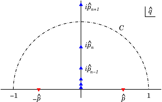
Figure 1: The contour $C$ in the complex $\hat{q}$-plane used to construct the solution $\hat{\jmath}(\hat{p},\Lambda)$ of the DWRG equation. The bound-state poles of the integrand occur at $\hat{q}=i\hat{p}_{n}=ip_{*}e^{n\pi/s_{\scriptscriptstyle 0}}/\Lambda$ and the propagator poles at $\hat{q}=\pm\hat{p}$.

Fig. 1 also shows the pole structure of the integrand $h(\hat{q})$. Apart from the two propagator poles at $\hat{q}=\pm\hat{p}$, there are bound-state poles at

$$\hat{q}=i\hat{p}_{n}(\Lambda)=i\,\frac{p_{*}}{\Lambda}\,e^{n\pi/s_{\scriptscriptstyle 0}}.$$ (24)

These poles are important since their positions vary with $\Lambda$ and so they can cross our integration contour. When this happens they generate discontinuities in $\hat{\jmath}(\hat{p},\Lambda)$. By choosing our contour to cross the imaginary axis at $\hat{q}=i$ (corresponding to an energy $E=-\Lambda^{2}/M$) we can arrange for these discontinuities to match precisely the ones we require in Eq. (15). To see this, note that as $\Lambda$ is varied from $p_{n}-\epsilon$ to $p_{n}+\epsilon$, the pole at $\hat{q}=i\hat{p}_{n}$ crosses the contour and produces a discontinuity

$$\Bigl{[}\hat{\jmath}(\hat{p},\Lambda)\Bigr{]}_{\Lambda=p_{n}-\epsilon}^{\Lambda=p_{n}+\epsilon}=-2\pi i\,{\cal R}\left[h(\hat{q}),i\hat{p}_{n}\right]=\frac{\pi}{s_{\scriptscriptstyle 0}}\,\frac{1}{1+\hat{p}^{2}},$$ (25)

where ${\cal R}[f(z),z_{0}]$ denotes the residue of $f(z)$ at the pole $z_{0}$. This is precisely the strength of the $\delta$-function at $p_{n}(\Lambda)=1$ in Eq. (15).

The integral $\hat{\jmath}(\hat{p},\Lambda)$ satisfies the full RG equation (15) and is analytic about $\hat{p}^{2}=0$. We therefore define the rescaled potential by

$$\hat{v}_{3}^{(0)}(\hat{p},\Lambda)=\bigl{[}\hat{\jmath}(\hat{p},\Lambda)\bigr{]}^{-1}.$$ (26)

This is not a fixed point since it does depend logarithmically on $\Lambda$, but in it these logarithms have been resummed to all orders. The invariance of the system under Eq. (7) means that this dependence on $\ln\Lambda$ is periodic. As pointed out by Wilson wilslc , this periodic behaviour provides an example of a limit cycle of the RG.

Like a fixed point, the limit-cycle solution can be used to define a power counting for the perturbations around it. Because the RG equation in the form of Eq. (15) is linear in $1/\hat{v}_{3}$, it is possible to construct exact solutions containing these perturbations,

$$\frac{1}{\hat{v}_{3}(\hat{p},\Lambda)}=\frac{1}{\hat{v}_{3}^{(0)}(\hat{p},\Lambda)}+\sum_{n=0}^{\infty}C_{2n}\Lambda^{2n}\hat{p}^{2n}.$$ (27)

The perturbations around the cycle thus have exactly the same power counting as those around the trivial fixed point. The leading, energy-independent term is marginal. Each additional power of energy ($\hat{p}^{2}$) gives a term two orders higher in $\Lambda$.

The general solution, Eq. (27), shows that there is a family of limit cycles parameterised by the marginal perturbation $C_{0}$. This lack of uniqueness arises because the marginal perturbation is $\Lambda$-independent and satisfies the homogeneous version of the RG equation (15). As a result, an arbitrary amount of it can be added to the limit-cycle solution, Eq. (26). The leading perturbation around any cycle is marginal because it pushes the solution into a nearby cycle. In the limit $C_{0}\rightarrow\infty$, the entire cycle is compressed into the trivial fixed point $\hat{v}_{3}=0$, which can be regarded as the limiting member of the family of cycles. All other perturbations vanish as $\Lambda\rightarrow 0$ and hence are stable. Any more general solution will thus tend to one of the limit cycles as $\Lambda\rightarrow 0$.

Each limit cycle contains one discontinuity every period, when a bound state is removed from the low-energy domain. The point in the cycle where this occurs depends on how we truncate the sum over bound states. Here we have chosen a cut-off that is symmetric between positive and negative energies, although other prescriptions are equally acceptable since physical observables should not depend on them.

The truncation of bound states ensures that our solution of the RG equation is single-valued. Our choice corresponds to a particular path from $\hat{q}=-1$ to $+1$ for the contour $C$ used to evaluate $\hat{\jmath}(\hat{p},\Lambda)$. Other, topologically different paths would correspond to different branches of a general multi-valued solution. Such multi-valuedness appears in other methods used to renormalise the three-body potential, as in Refs. bhvk ; bbh ; hm ; bghr .

III.3 Scattering observables

To relate the parameters appearing in our solution, Eq. (27), to scattering observables, we need to construct the corresponding $T$-matrix. If we use the separable form of the wave functions, we can define a DW $T$-matrix $\tilde{t}_{3}$ in an analogous manner to Eq. (12). Projecting the LS equation Eq. (3) onto the $s_{0}$ channel, we get the correspondimng equation for $\tilde{t}_{3}$. With our choice of energy-dependent potential, this can be solved directly to get the on-shell $T$-matrix,

$$\langle u^{-}_{p}|\tilde{t}_{3}(p)|u^{+}_{p}\rangle=e^{2i\delta_{2}(p)}|u_{p}(\bar{R})|^{2}v_{3}(p,\Lambda)\left[1-g_{2}(p,\Lambda;\bar{R},\bar{R})v_{3}(p,\Lambda)\right]^{-1},$$ (28)

where the superscripts $\pm$ denote waves with incoming or outgoing boundary conditions, and $\delta_{2}$ is the phase shift in the $s_{\scriptscriptstyle 0}$ channel produced by the pairwise forces alone.

Unitarity and conservation of hyperangular momentum allow us to express this in terms of a phase-shift as

$$\frac{e^{2i\delta_{2}(p)}}{\langle u^{-}_{p}|\tilde{t}_{3}(p)|u^{+}_{p}\rangle}=-\frac{M}{2\pi p}\bigl{(}\cot\tilde{\delta}_{3}(p)-i\bigr{)}.$$ (29)

Here $\tilde{\delta}_{3}$ is the additional phase shift produced by the three-body force. It is related to the full phase shift $\delta$ by $\tilde{\delta}_{3}=\delta-\delta_{2}$. Using the fact that our potential acts at $R=\bar{R}$, we can combine Eqs.(28, 29) to obtain an equation relating $v_{3}$ and the phase shift:

$$|u_{p}(\bar{R})|^{2}\frac{M}{2\pi p}(\cot{\tilde{\delta}_{3}}-i)=g_{2}(p,\Lambda;\bar{R},\bar{R})-v_{3}(p,\Lambda)^{-1}.$$ (30)

When we use the expression in Eq. (10) for the regularised Green’s function and the explicit forms of the wave functions from Appendix A, we find that the $\bar{R}$ dependence can be factored out to leave

$$\frac{\pi}{2}\left(\frac{\sinh(\pi s_{\scriptscriptstyle 0})}{\cosh(\pi s_{\scriptscriptstyle 0})-\cos\bigl{(}2s_{\scriptscriptstyle 0}\ln(p/p_{*})\bigr{)}}\right)\bigl{(}\cot{\tilde{\delta}_{3}(p)}-i\bigr{)} = \int_{0}^{\Lambda}\frac{q\sinh(\pi s_{\scriptscriptstyle 0})dq}{\bigl{[}\cosh(\pi s_{\scriptscriptstyle 0})-\cos\bigl{(}2s_{\scriptscriptstyle 0}\ln(q/p_{*})\bigr{)}\bigr{]}(p^{2}-q^{2}+i\epsilon)}$$ (31)

$$\qquad\quad+\frac{\pi}{s_{\scriptscriptstyle 0}}\sum_{|p_{n}|<\Lambda}\frac{p_{n}^{2}}{p^{2}+p_{n}^{2}}-\frac{1}{\hat{v}_{3}(p/\Lambda,\Lambda)}.$$

To write this in a form which is explicitly independent of $\Lambda$, we introduce the rescaled variable $\hat{q}=q/\Lambda$ and substitute in our solution for $\hat{v}_{3}$ from Eq. (27). This gives

$$\frac{\pi}{2}\left(\frac{\sinh(\pi s_{\scriptscriptstyle 0})}{\cosh(\pi s_{\scriptscriptstyle 0})-\cos\bigl{(}2s_{\scriptscriptstyle 0}\ln(p/p_{*})\bigr{)}}\right)\bigl{(}\cot{\tilde{\delta}_{3}(p)}-i\bigr{)}=\int_{-1}^{1}d\hat{q}\,h(\hat{q})-\int_{C}d\hat{q}\,h(\hat{q})-2\pi i\sum_{|p_{n}|<\Lambda}{\cal R}\left[h(\hat{q}),ip_{n}/\Lambda\right]-\sum_{n=0}^{\infty}C_{2n}p^{2n},$$ (32)

where $h(\hat{q})$ is defined above in Eq. (21) and we used the fact that the sum over the bound states can be expressed in terms of the residues at the bound-state poles (see Eq. (25)).

The two integrals over $h(\hat{q})$ can be combined to form a single integral round a closed contour. The $i\epsilon$ prescription in the first integral implies that the contour of integration goes above the propagator pole at $\hat{q}=-\hat{p}$ and below the one at $\hat{q}=\hat{p}$. The contour thus encloses the pole at positive $\hat{q}$. It also encloses the bound state poles at $\hat{q}=ip_{n}/\Lambda$ with $p_{n}<\Lambda$. Using Cauchy’s theorem, we find that the residues from these exactly cancel the sum over bound states in Eq. (32).

We are then left with a DW effective-range expansion,

$$\left(\frac{\sinh(\pi s_{\scriptscriptstyle 0})}{\cosh(\pi s_{\scriptscriptstyle 0})-\cos\bigl{(}2\eta(p)\bigr{)}}\right)\bigl{(}\cot{\tilde{\delta}_{3}(p)}-i\bigr{)}=\cot\left(\eta(p)+\frac{i\pi s_{\scriptscriptstyle 0}}{2}\right)-\frac{2}{\pi}\sum_{n=0}^{\infty}C_{2n}p^{2n},$$ (33)

where $\eta(p)=-s_{\scriptscriptstyle 0}\ln(p/p_{*})$ is defined in Eq. (76). Make use of trigonometric additon fomulae, one can show that the imaginary parts of the left and right sides are equal. In this expansion, all nonanalytic behaviour has been subtracted or factored out into the trigonometric functions of $\ln p$. The remaining energy dependence can be expanded in powers of $p^{2}$ and the terms correspond directly to perturbations around the limit cycle.

The roles of the limit-cycle potential and its marginal perturbation $C_{0}$ are not obvious from Eq. (33) and so, to clarify these, we construct the total phase shift, $\delta$. Making use of Eqs. (33) and (77), the corresponding full $S$-matrix can be written

$$e^{2i\delta(p)}=i\frac{Z^{*}(p)}{Z(p)},$$ (34)

where

$$\qquad Z(p)=\cos\left(\eta(p)+\frac{i\pi s_{\scriptscriptstyle 0}}{2}\right)-\frac{2}{\pi}\,\sin\left(\eta(p)+\frac{i\pi s_{\scriptscriptstyle 0}}{2}\right)\sum_{n=0}^{\infty}C_{2n}p^{2n}.$$ (35)

For the limit-cycle solution of Eq. (26) with no perturbations (all $C_{2n}=0$), we have

$$Z(p)=\cos\left(\eta(p)+\frac{i\pi s_{\scriptscriptstyle 0}}{2}\right).$$ (36)

Comparing this to Eq. (77) for the pure long-range force, we see that the phase $\eta(p)$ of the waves near the origin has been shifted by $\pi/2$. This implies, for example, that the bound states lie at $p=ie^{-\pi/2s_{\scriptscriptstyle 0}}p_{n}$, which correspond to the geometric means of the bound state energies for $v_{3}=0$. This potential thus corresponds to the system which is “furthest away” from the one with $v_{3}=0$, in the sense that it leads to the maximum possible changes to physical observables.

To elucidate the role of the marginal perturbation, it is convenient to express its coefficient in terms of an angle $\sigma$,

$$C_{0}=-\frac{\pi}{2}\cot\sigma,$$ (37)

and to redefine the other short-distance parameters according to

$$\frac{2}{\pi}\sum_{n=1}^{\infty}C_{2n}p^{2n}=\frac{\csc\sigma\sum_{n=1}^{\infty}C^{\prime}_{2n}p^{2n}}{\sin\sigma+\cos\sigma\sum_{n=1}^{\infty}C^{\prime}_{2n}p^{2n}}.$$ (38)

In terms of the new parameters, $\sigma$ and $C^{\prime}_{2n}\,,n\geq 1$ we find that the $S$-matrix can still be written in the form of Eq. (34), but with $Z(p)$ replaced by

$$Z^{\prime}(p)=\sin\left(\eta(p)+\sigma+\frac{i\pi s_{\scriptscriptstyle 0}}{2}\right)+\cos\left(\eta(p)+\sigma+\frac{i\pi s_{\scriptscriptstyle 0}}{2}\right)\sum_{n=1}^{\infty}C^{\prime}_{2n}p^{2n}.$$ (39)

This form makes it clear that $\sigma$ (or rather $C_{0}$) just has the effect of shifting the phase $\eta(p)$. Scattering observables depend only on the combination

$$p^{\prime}_{*}=e^{-\sigma/s_{\scriptscriptstyle 0}}p_{*},$$ (40)

and not on $p_{*}$ and $C_{0}$ separately. This shows that $p_{*}$ and $C_{0}$ play the same role in determining the phase of the wave functions for $R\rightarrow 0$ (the self-adjoint extension of the Hamiltonian). We can use $C_{0}$ to change the self-adjoint extension from the initial one specified by $p_{*}$ to any other. In particular, $\sigma=0$ (corresponding to the trivial fixed point) leaves the initial extension unchanged, whereas $\sigma=\pi/2$ ($C_{0}=0$) produces the largest possible change in the extension, as already noted. Furthermore, there is a one-to-one mapping between all possible limit-cycle solutions (obtained by varying $C_{0}$ from $-\infty$ to $+\infty$ or equivalently $\sigma$ between $0$ and $\pi$) and the self-adjoint extensions. This is in marked contrast to the relationship between $p_{*}$ and the self-adjoint extensions, where infinitely many equivalent $p_{*}$’s give the same extension.

The bound states of the system are given by the zeros of $Z^{\prime}(p)$. For any short-range potential, the bound states still accumulate at zero energy, as expected since they are consequences of the inverse-square tail of the long-range potential. The shallower bound states are insensitive to the short-range perturbations, $C^{\prime}_{2n}$ with $n\geq 1$. Their positions are controlled by $p^{\prime}_{*}$ rather than the original $p_{*}$. If we choose $p_{*}$ to give the correct shallow Efimov states, we can set $\sigma=0$ and use the expansion around the trivial fixed point. This corresponds to expanding a DW $K$-matrix and has the form

$$\frac{\tan\tilde{\delta}_{3}(p)}{\sinh(\pi s_{\scriptscriptstyle 0})}=\frac{\sum_{n=1}^{\infty}C^{\prime}_{2n}p^{2n}}{\cosh(\pi s_{\scriptscriptstyle 0})-\cos\bigl{(}2\eta(p)\bigr{)}+\sin\bigl{(}2\eta(p)\bigr{)}\sum_{n=1}^{\infty}C^{\prime}_{2n}p^{2n}}.$$ (41)

The deeper bound states are of course strongly affected by the higher-order perturbations and will not in general follow the simple constant-ratio pattern of the Efimov states. At some point they will fall outside the range of validity of the EFT and so we can say nothing about them, except that some short-range physics must act to ensure the existence of a ground state.

IV Finite Scattering Length

In the general case of finite scattering length it no longer makes sense to expand observables in terms of the hyperangular wavefunctions, instead we must consider a much more general RG equation. In particular, the low-energy scales now include $\gamma=1/a_{2}$ where $a_{2}$ is the two body scattering length. This can also be thought of as the typical momentum in the low-lying bound or virtual state of two particles. The coupling between waves with different hyperangular momenta means that the states should now depend on the relative momentum $k$ of a pair, as well as the total energy, expressed as a momentum $p$. Nonetheless Efimov’s separation of variables still applies whenever the distances between the three particles are all much less than the two-body scattering length efimov . It therefore controls the short-distance behaviour of the three-body wave function in an EFT with contact interactions and hence the scaling of the short-range three-body interactions. For attractive three-body systems, the the basic structure of the RG evolution will be similar to that in the previous section since the wave functions at small $R$ will still be dominated by the $s_{\scriptscriptstyle 0}$ channel.

The truncated Green’s function is given by Eq. (1) restricted to states inside the energy range $-\Lambda^{2}/M\leq E\leq\Lambda^{2}/M$:

$$G_{2}(p)=\frac{M}{4\pi}\sum_{|p_{n}|<\Lambda}\frac{|\Psi_{n}\rangle\langle\Psi_{n}|}{p^{2}+p_{n}^{2}}+\frac{M}{2\pi^{2}}\int_{-\gamma^{2}}^{\Lambda^{2}}d(q^{2})\frac{1}{p^{2}-q^{2}+i\epsilon}\left[|\Psi_{q,i\gamma}\rangle\langle\Psi_{q,i\gamma}|+\vartheta(q^{2})\frac{2}{\pi}\int_{0}^{q}dk|\Psi_{q,k}\rangle\langle\Psi_{q,k}|\right].$$ (42)

Inserting this into Eq. (5) and using Eq. (4) we obtain a differential equation for the potential

$$\frac{\partial V_{3}(p,\gamma,k,k^{\prime};\Lambda)}{\partial\Lambda} = -\,\frac{M\bar{R}^{4}}{2\pi^{2}}\frac{1}{p^{2}-\Lambda^{2}}\Biggl{[}V_{3}(p,\gamma,k,i\gamma;\Lambda)|\Psi_{\Lambda,i\gamma}(\bar{R},\bar{\Omega})|^{2}V_{3}(p,\gamma,i\gamma,k^{\prime};\Lambda)$$ (43)

$$\qquad\qquad\qquad+\frac{2}{\pi}\int_{0}^{\Lambda}dk^{\prime\prime}V_{3}(p,\gamma,k,k^{\prime\prime};\Lambda)|\Psi_{\Lambda,k^{\prime\prime}}(\bar{R},\bar{\Omega})|^{2}V_{3}(p,\gamma,k^{\prime\prime},k^{\prime};\Lambda)\Biggr{]}$$

$$-\frac{M\bar{R}^{4}}{4\pi}\sum_{n=0}^{\infty}\frac{|\Psi_{n}(\bar{R},\bar{\Omega})|^{2}}{p^{2}+p_{n}^{2}}\,\delta(\Lambda-p_{n})V_{3}(p,\gamma,k,ip_{n}/3;\Lambda)V_{3}(p,\gamma,ip_{n}/3,k^{\prime};\Lambda).$$

For $R\ll a_{2}$ all the DW’s will be dominated by the $s_{\scriptscriptstyle 0}$ channel and will therefore tend to the forms

$$|\Psi_{p,k}(R,\Omega)|^{2} \sim \frac{1}{p}{\cal D}_{3}(p,k,\gamma,p_{*})\,|\xi(\Omega)|^{2}\frac{\sin^{2}\left(s_{\scriptscriptstyle 0}\ln(p_{*}R)-\theta\right)}{R^{4}},$$

$$|\Psi_{p,i\gamma}(R,\Omega)|^{2} \sim {\cal D}_{2}(p,\gamma,p_{*})\,|\xi(\Omega)|^{2}\frac{\sin^{2}\left(s_{\scriptscriptstyle 0}\ln(p_{*}R)-\theta\right)}{R^{4}},$$

$$|\Psi_{n}(R,\Omega)|^{2} \sim p_{n}^{2}\,{\cal D}_{B}^{(n)}(\gamma,p_{*})\,|\xi(\Omega)|^{2}\frac{\sin^{2}\left(s_{\scriptscriptstyle 0}\ln(p_{*}R)-\theta\right)}{R^{4}}.$$ (44)

The various normalisation functions, ${\cal D}_{3}$, ${\cal D}_{2}$ and ${\cal D}_{B}^{(n)}$, are determined by the external boundary conditions on the DW’s. They can be found by solving the full Faddeev equations (or equivalents). These functions are essential to the RG discussion, since it is through them that information about the long-distance physics is communicated to short distances.

The forms of the DW’s above were chosen to ensure that the normalisation functions are dimensionless. They have a common dependence on the hyperangles given by the function

$$\xi(\Omega)={\cal A}_{s_{0}}\sum_{i=1}^{3}\frac{2}{\sin(2\varphi_{i})}\sinh\left(\frac{s_{0}\pi}{2}-s_{0}\varphi_{i}\right),$$ (45)

where $\varphi_{i}$ is the hyperangle defined in appendix A. Since this dependence can be factored out of the Green’s function $G_{2}(p)$ at small $R$, it is unimportant to the RG discussion. In this context, it is convenient to define a Green’s function with this common short-distance behaviour divided out,

$${\cal G}_{2}(p,\gamma,p_{*})=\frac{2\pi^{2}\bar{R}^{4}}{M}\frac{G_{2}(p;\bar{R},\bar{\Omega};\bar{R},\bar{\Omega})}{|\xi(\bar{\Omega})|^{2}\sin^{2}\left(s_{\scriptscriptstyle 0}\ln(p_{*}\bar{R})-\theta\right)}.$$ (46)

Using the forms of the DW’s given in Eq. (44) we define our rescaled potential by

$$\hat{V}_{3}(\hat{p},\hat{\gamma},\hat{k},\hat{k}^{\prime};\Lambda)=\frac{M}{2\pi^{2}}|\xi(\bar{\Omega})|^{2}\sin^{2}\bigl{(}s_{\scriptscriptstyle 0}\ln(p_{*}\bar{R})-\theta\bigr{)}V_{3}(p,\gamma,k,k^{\prime};\Lambda),$$ (47)

where, as usual, $\hat{p}=p/\Lambda$, etc. We also require rescaled versions of the normalisation functions $\cal D$, which we define by

$$\hat{\cal D}_{3}(\hat{k},\hat{\gamma},\Lambda)={\cal D}_{3}(\Lambda,\Lambda\hat{k},\Lambda\hat{\gamma},p_{*}),\qquad\hat{\cal D}_{2}(\hat{\gamma},\Lambda)={\cal D}_{2}(\Lambda,\Lambda\hat{\gamma},p_{*}),\qquad\hat{\cal D}_{B}^{(n)}(\hat{\gamma},\Lambda)={\cal D}_{B}^{(n)}(\Lambda\hat{\gamma},p_{*}),$$ (48)

Since $p_{*}$ only occurs in these dimensionless functions as a ratio with $\Lambda$ (the only other scale) we have suppressed the dependence on it to simplify notation. We also define a similarly rescaled Green’s function,

$$\hat{\cal G}_{2}(\hat{\gamma},\Lambda)={\cal G}_{2}(\Lambda,\Lambda\hat{\gamma},p_{*}).$$ (49)

The rescaled potential $\hat{V}_{3}$ satisfies the RG equation

$$\Lambda\frac{\partial\hat{V}_{3}}{\partial\Lambda} = \hat{p}\frac{\partial\hat{V}_{3}}{\partial\hat{p}}+\hat{\gamma}\frac{\partial\hat{V}_{3}}{\partial\hat{\gamma}}+\hat{k}\frac{\partial\hat{V}_{3}}{\partial\hat{k}}+\hat{k}^{\prime}\frac{\partial\hat{V}_{3}}{\partial\hat{k}^{\prime}}$$ (50)

$$+\frac{1}{1-\hat{p}^{2}}\Biggl{[}\hat{V}_{3}(\hat{p},\hat{\gamma},\hat{k},i\hat{\gamma};\Lambda)\hat{\cal D}_{2}(\hat{\gamma},\Lambda)\hat{V}_{3}(\hat{p},\hat{\gamma},i\hat{\gamma},\hat{k}^{\prime};\Lambda)$$

$$\qquad\qquad+\frac{2}{\pi}\int_{0}^{1}d\hat{k}^{\prime\prime}\hat{V}_{3}(\hat{p},\hat{\gamma},\hat{k},\hat{k}^{\prime\prime};\Lambda)\hat{\cal D}_{3}(\hat{k}^{\prime\prime},\hat{\gamma},\Lambda)\hat{V}_{3}(\hat{p},\hat{\gamma},\hat{k}^{\prime\prime},\hat{k}^{\prime};\Lambda)\Biggr{]}$$

$$+\frac{\pi}{2}\sum_{n=0}^{\infty}\hat{\cal D}_{B}^{(n)}(\hat{\gamma},\Lambda)\frac{1}{1+\hat{p}^{2}}\delta(\hat{p}_{n}(\Lambda)-1)\hat{V}_{3}(\hat{p},\hat{\gamma},\hat{k},i\hat{p}_{n}/3;\Lambda)\hat{V}_{3}(\hat{p},\hat{\gamma},i\hat{p}_{n}/3,\hat{k}^{\prime};\Lambda).$$

The boundary conditions on $\hat{V}_{3}$ are that it be analytic in $\hat{p}^{2}$, $\hat{\gamma}$, $\hat{k}^{2}$ and $\hat{k}^{\prime 2}$. Again these follow from our requirement that the potential arises from six-point contact terms in the effective Lagrangian.

Note that in the $\hat{\cal D}$’s and the rescaled bound-state momenta $\hat{p}_{n}(\Lambda)$ the only explicit dependence on $\Lambda$ occurs in the ratio $\Lambda/p_{*}$. (The scales $p_{*}$ and $\Lambda$ are the only ones in these dimensionless functions.) The scale $p_{*}$ is introduced, as before, by the self-adjoint extension which fixes the phase of the waves for $R\rightarrow 0$. All quantities appearing in the RG equation are thus invariant under the transformation of $p_{*}$ in Eq. (7) and hence are periodic in $p_{*}$. Furthermore, since $p_{*}$ and $\Lambda$ always appear as a ratio in the RG equation, that equation must be unchanged under

$$\Lambda\rightarrow\Lambda e^{-n\pi/s_{\scriptscriptstyle 0}},\qquad n\in\mathbb{Z}.$$ (51)

In interpreting this for the bound state momenta $\hat{p}_{n}(\Lambda)$ we need to be careful. Depending on how we label the states, these momenta may not obey the symmetry individually. However the complete set must always obey it collectively.

To see how this happens, consider the entire rescaled spectrum, $\hat{p}_{n}$, at some initial scale $\Lambda=\Lambda_{1}$. As $\Lambda$ decreases the rescaled bound state momenta increase, until at $\Lambda=\Lambda_{1}e^{-\pi/s_{\scriptscriptstyle 0}}$ the spectrum has shifted so that $\hat{p}_{n}(\Lambda)=\hat{p}_{n+1}(\Lambda^{\prime})$. This is similar to what happened in the case of infinite scattering length, except that a new bound state must have appeared at threshold and moved down to $\hat{p}_{0}(\Lambda_{1})$. This is possible because in following the RG flow we keep the rescaled quantity $\hat{\gamma}$ fixed, not the physical value $\gamma$. The spectrum at $\Lambda=\Lambda_{1}e^{-\pi/s_{\scriptscriptstyle 0}}$ is thus identical to that at $\Lambda_{1}$. If we label the bound states so that $\hat{p}_{0}(\Lambda)$ always refers to the shallowest, then each of the $\hat{p}_{n}(\Lambda)$ will be invariant under Eq. (51).

The general RG equation is complicated because it includes couplings between the different three-body channels. As a starting point for solving this equation, we consider a solution which is independent of the two relative momenta, $\hat{k}$ and $\hat{k}^{\prime}$. This simplifies the equation considerably since it allows us to divide through by $\hat{V}_{3}(\hat{p},\hat{\gamma};\Lambda)^{2}$ to obtain a linear equation for $1/\hat{V}_{3}$,

$$\displaystyle{\Lambda\frac{\partial}{\partial\Lambda}\left(\frac{1}{\hat{V}_{3}}\right)=\hat{p}\frac{\partial}{\partial\hat{p}}\left(\frac{1}{\hat{V}_{3}}\right)+\hat{\gamma}\frac{\partial}{\partial\hat{\gamma}}\left(\frac{1}{\hat{V}_{3}}\right)-\frac{1}{1-\hat{p}^{2}}\hat{P}(\hat{\gamma},\Lambda)+\frac{\pi}{2}\sum_{n=0}^{\infty}\hat{\cal D}_{B}^{(n)}(\hat{\gamma},\Lambda)\frac{1}{1+\hat{p}^{2}}\delta(\hat{p}_{n}(\Lambda)-1),}$$ (52)

where we have introduced the function

$$\hat{P}(\hat{\gamma},\Lambda)=\hat{\cal D}_{2}(\hat{\gamma},\Lambda)+\frac{2}{\pi}\int_{0}^{1}d\hat{k}^{\prime\prime}\hat{\cal D}_{3}(\hat{k}^{\prime\prime},\hat{\gamma},\Lambda).$$ (53)

This function can be thought of as the (rescaled) short-distance part of the projection operator onto continuum states with energy $E=\Lambda^{2}/M$.

Our strategy for solving Eq. (52) will mirror that used in the simpler case of infinite scattering length. As before, we can immediately write down a solution to the continuous equation using an equivalent to the basic loop integral, Eq. (19). Again this will not satisfy the analyticity boundary conditions because of the behaviour of the integrand at the endpoint $\hat{q}=0$. Furthermore this solution will not generate the discontinuities at the bound states. We must therefore find a generalisation of Eq. (20) and write the solution as a contour integral that avoids the point $\hat{q}=0$.

Guided by the results for infinite scattering length, we define an integral along the same contour $C$ as before,

$$\hat{J}(\hat{p},\hat{\gamma},\Lambda)=\int_{C}d\hat{q}\,H(\hat{q}),$$ (54)

where

$$H(\hat{q})=\frac{i}{\pi}\frac{\hat{q}}{\hat{p}^{2}-\hat{q}^{2}}\,\hat{\cal G}_{2}(\hat{\gamma}/\hat{q},\hat{q}\Lambda).$$ (55)

The contour $C$ is shown in Fig. 2 along with the singularity structure of $H$. This structure follows straightforwardly from the form of $\hat{\cal G}_{2}$ and is derived in appendix B.

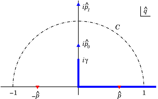
Figure 2: The contour $C$ used to construct the DWRG solution $\hat{J}(\hat{p},\hat{\gamma},\Lambda)$. The bound-state poles of the integrand $H(\hat{q})$ occur at $\hat{q}=i\hat{p}_{n}$. The branch cut running down the imaginary axis corresponds to the $2+1$ elastic continuum. This is joined by a cut starting at $\hat{q}=0$ corresponding to the three-body continuum. There are also propagator poles at $\hat{q}=\pm\hat{p}$.

In appendix B we also show that the function $\hat{P}(\hat{\gamma},\Lambda)$ in Eq. (52) can be rewritten in terms of $\hat{\cal G}_{2}$ as

$$\hat{P}(\hat{\gamma},\Lambda)=\frac{i}{\pi}\Bigl{(}\hat{\cal G}_{2}(\hat{\gamma},\Lambda)-\hat{\cal G}_{2}(-\hat{\gamma},-\Lambda)\Bigr{)}.$$ (56)

This result can then be used to show that $\hat{J}(\hat{p},\hat{\gamma},\Lambda)$ satisfies the continuous part of Eq. (52). In addition, the bound state poles in $H$ cross the contour of integration at $\hat{p}_{n}=1$ and so produce the necessary discontinuities. Finally, the contour never approaches the branch points at $\hat{q}=0$ and $\hat{q}=i\hat{\gamma}$ and so the integral is analytic in the small scales. This allows us to take our nontrivial solution to the DWRG equation to be

$$\hat{V}_{3}^{(0)}(\hat{p},\hat{\gamma},\Lambda)=\bigl{[}\hat{J}(\hat{p},\hat{\gamma},\Lambda)\bigr{]}^{-1}.$$ (57)

The periodic dependence on $\Lambda$ of all quantities appearing the DWRG equation (52) implies that our solution $\hat{V}_{3}^{(0)}(\hat{p},\hat{\gamma},\Lambda)$ must also be periodic. Like the analogous solution for infinite scattering length, it is therefore a limit-cycle of the DWRG.

As a result, it must have an infinite number of discontinuities as $\Lambda\rightarrow 0$, which follow a periodic pattern according to this symmetry. At first glance this may seem odd since these discontinuities are associated with the truncation of bound states and there are only a finite number of bound states in the truncated Green’s function. However as $\Lambda$ is lowered for fixed $\hat{\gamma}$, new bound states appear in the rescaled spectrum as discussed above

Now that we have obtained a limit-cycle solution, the analysis proceeds along very similar lines to that in the previous section. The perturbations in $\hat{p}$ and $\hat{\gamma}$ are simple to derive and, since Eq. (52) is linear, they give exact solutions to the DWRG equation:

$$\frac{1}{\hat{V}_{3}(\hat{p},\hat{\gamma},\Lambda)}=\frac{1}{\hat{V}_{3}^{(0)}(\hat{p},\hat{\gamma},\Lambda)}+\sum_{n,m=0}^{\infty}C_{2n,m}\Lambda^{2n+m}\hat{p}^{2n}\hat{\gamma}^{m}.$$ (58)

The main features of the power-counting are unaffected by the addition of the new scale $\gamma$. The LO perturbation is still marginal, and leads to a family of limit-cycles parametrised by $C_{0,0}$. Although it is more difficult to show, the analysis of the infinite-scattering-length case suggests that the marginal perturbation $C_{0,0}$ and the scale $p_{*}$ must represent the same three-body physics in the EFT.

The previous power-counting is supplemented by terms proportional to powers of $\gamma$. In many systems, such as those of interest in nuclear physics, the two-body scattering lengths and hence $\gamma$ are fixed. This means that these terms can not be determined separately but must be absorbed into the coefficients of the energy-dependent perturbations. However in atomic systems with tunable Feshbach resonances, it may be possible to vary $\gamma$ and hence to disentangle the energy- and $\gamma$-dependent perturbations.

The full set of perturbations also includes ones that depend on the relative momenta. The forms of these have been derived and their eigenvalues show that they occur at the same orders as the corresponding energy-dependent perturbations. The full expressions are very unwieldy and so the interested reader is referred to Ref. tbthesis .

Having obtained a solution to the RG equation we can substitute it back into the LS equation to obtain the corresponding DW $T$-matrix. The algebra again follows that for systems with infinite scattering length. In the present case, the truncated Green’s function involves an integral around the branch cut corresponding to elastic scattering of a single particle on a bound pair below the three-body threshold. This $2+1$ continuum cut runs along the imaginary $\hat{q}$-axis from $i\hat{\gamma}$, as shown in Fig. 2. Using the form for the three-body force given in Eq. (58) we find that the DW $T$-matrix element for $2+1$ elastic scattering can be written

$$\frac{2\pi^{2}}{M}\,\frac{{\cal D}_{2}(p,\gamma,p_{*})e^{2i\delta_{2}(p)}}{\langle\Psi^{-}_{p,i\gamma}|\tilde{T}_{3}(p)|\Psi^{+}_{p,i\gamma}\rangle}=-{\cal G}_{2}(p,\gamma,p_{*})+\sum_{n,m=0}^{\infty}C_{2n,m}p^{2n}\gamma^{m}.$$ (59)

Using the properties of ${\cal G}_{2}$ in Appendix B, one can show that $\tilde{T}_{3}(p)$ respects unitarity for $p^{2}<0$, as it should. For $p^{2}>0$, the coupling to three-body breakup channels, mean that $T$-matrix for $2+1$ scattering does not repect unitarity on its own. The same effective potential could be used to calculate amplitudes for breakup and $3\rightarrow 3$ scattering. However, in practice this is likely to require general momentum-dependent potentials to describe all possible interaction channels.

The DW $T$-matrix can be related to the elastic-scattering phase shift, $\delta$, by

$$\frac{e^{2i\delta_{2}(p)}}{\langle\Psi^{-}_{p,i\gamma}|\tilde{T}_{3}(p)|\Psi^{+}_{p,i\gamma}\rangle}=-\frac{M}{4\pi}\bigl{[}\cot\bigl{(}\delta(p)-\delta_{2}(p)\bigr{)}-i\bigr{]},$$ (60)

where $\delta_{2}$ is the phase shift produced by pairwise forces only. This allows us to rewrite Eq. (59) in the form of a DW effective-range expansion,

$$\frac{\pi}{2}\,{\cal D}_{2}(p,\gamma,p_{*})\bigl{[}\cot\bigl{(}\delta(p)-\delta_{2}(p)\bigr{)}-i\bigr{]}-{\cal G}_{2}(p,\gamma,p_{*})=-\sum_{n,m=0}^{\infty}C_{2n,m}p^{2n}\gamma^{m}.$$ (61)

V Discussion

In this paper we have applied a DW version of the RG to three-body scattering. This is based on cutting off the full solutions in the presence of long-range interactions bb1 . In three-body systems, these long-range forces are generated by point-like interactions between pairs of particles. By imposing the cut-off on the DW’s we ensure that it affects only the contributions of the short-range three-body forces, and does not alter the two-body physics. Demanding that observables are independent of the cut-off then leads to an RG equation for the renormalised three-body interactions.

As shown by Efimov efimov , a three-body system with contact interactions can be described by an ISP in the region where they are all close together. Hence the RG in presence of this rather singular potential controls the behaviour of the three-body forces and determines their power counting.

For systems of three bosons or two neutrons and a proton with total spin $\frac{1}{2}$, the resulting ISP is attractive. This leads to quite different behaviour compared with previous examples studied with this type of RG bmr ; bb1 . The wave functions show oscillatory behaviour at short distances and a self-adjoint extension is needed to fix their phase and hence give well-defined eigenfunctions meetz ; case ; pp ; bc . These oscillatory functions control the RG flow of the short-distance potential, which tends to a limit cycle wilslc rather than a nontrivial fixed point.

These results are general for an attractive ISP in any number of dimensions. The lack of a ground state for such a potential means that it has deeply bound states that lie outside the domain of validity of our effective theory. This means that the cut-off should truncate not only high-energy scattering states but also these deeply bound states. This leads to a three-body force that has periodic discontinuities, but is single-valued.

The resulting power counting for perturbations around the limit cycle starts with a marginal term. From its effect on observables, we have seen that this term is equivalent to changing the parameter in the self-adjoint extension or, in other words, the phase of the short-distance wave functions. To express the resulting power counting in a form which matches that usually used wein79 ; wein , we can assign an order $d=\mu-1$ to a term in the rescaled potential proportional to $\Lambda^{\mu}$. Then a term proportional to $p^{2n}$ (or $E^{n}$) appears at order $d=2n-1$. The coefficents in our potential have direct, and relatively simple, connection to scattering observables.

The same behaviour is found in an attractive three-body system with finite two-body scattering length, $a_{2}$, since the wave functions tend to the Efimov form at short distances ($R\ll a_{2}$). Hence the RG flow has a very similar pattern, tending to a limit cycle. In this case the power counting should be extended to include terms involving powers of the low-energy scale $\gamma=1/a_{2}$. A term proportional to $p^{2n}\gamma^{m}$ is of order $d=2n+m-1$. For the energy-dependent perturbations, this counting agrees with that found by Bedaque et al. bghr from the STM equation. Because of the clean separation of the short- and long-range physics in the DWRG approach we are able to state the counting in an algebraically much simpler way.

We are also able to extend the counting to terms involving powers of $\gamma$. This may not be relevant to applications in nuclear physics, where the two-body scattering lengths are fixed, but in atomic systems it may be possible to use Feshbach resonances to vary the scattering length, and hence to disentangle the two types of perturbation.

The leading, marginal three-body force, or equivalently the choice of self-adjoint extension, is of interest since it shows that one piece of three-body physics is needed to determine low-energy three-body observables. As noted by Bedaque et al. bhvk , this provides a way to understand the old observation of the “Phillips line,” a correlation between the $J=\frac{1}{2}$ $nd$ scattering lengths and triton binding energies predicted by model nucleon-nucleon potentials phillips .

At leading order ($d=-1$), three-body observables are determined by the two-body scattering length and the marginal three-body force. The first correction to this arises from the two-body effective range, which appears at order $d=0$. Including this has been shown to give good agreement with with $J=\frac{1}{2}$ $nd$ observables, in calculations using the STM equation bghr and an equivalent equation in coordinate-space tbthesis . The first energy-dependent three-body force appears only at next-to-next-to-leading order, $d=1$ in this counting.

It should be possible to extend our approach to three-body scattering above the breakup threshold. However this will introduce couplings between various channels and so will involve momentum-dependent perturbations in the effective potential. This is likely to require similar analyses to those which have been applied to simpler coupled-channel systems, such as that considered in Ref. cgvk .

Appendix A Efimov wave functions

We summarise here the essential elements of Efimov’s approach to the three-body problem efimov , since this provides the wave functions we need to elucidate the scaling of the the three-body interactions.

We consider the case of $s$-wave scattering. In general, the wavefunctions $|\Psi_{p,k}\rangle$ must be found using the Faddeev equations or equivalent (see, for example, Ref. m3hp ). In the Faddeev formalism, the wavefunction is broken into three components according to the pair of particles that interacted last. The component in which particles $2$ and $3$ interacted last is denoted $\psi^{(1)}_{p,k}(r_{23},r_{1})$, where $r_{23}$ and $r_{1}$ are the usual Jacobian coordinates for three bodies with equal masses.

For particles interacting via pairwise contact interactions, Efimov observed that $\psi^{(i)}_{p,k}(r_{jk},r_{i})$ satisfies a free two-dimensional Schrödinger equation, subject to a boundary condition relating the wave function at the points $r_{jk}=0$ and $r_{i}=r_{jk}/2$ where pairs of particles interact. This boundary condition takes the form

$$\left[\frac{\partial\psi^{(i)}_{p,k}(R,\varphi_{i})}{\partial\varphi_{i}}\right]_{\varphi_{i}=0}+\frac{8\lambda}{\sqrt{3}}\psi^{(i)}_{p,k}(R,\pi/3)=\frac{R}{a_{2}}\psi_{p,k}^{(i)}(R,0),$$ (62)

where $\lambda$ is a factor related to the wave-function symmetry, and $R$ and $\varphi_{i}$ are the hyperradius and hyperangle respectively, and are defined by

$$R=\sqrt{\frac{4}{3}r_{i}^{2}+r_{jk}^{2}},\qquad\varphi_{i}=\arctan{\frac{\sqrt{3}r_{jk}}{2r_{i}}}.$$ (63)

For three bosons, the full wavefunction can be expressed as

$$\Psi_{p,k}(R,\Omega)=\sum_{i=1}^{3}\frac{2}{R^{2}\sin(2\varphi_{i})}\psi^{(i)}_{p,k}(R,\varphi_{i}),$$ (64)

where $\Omega$ represents five general hyperspherical coordinates that complement $R$. (The other coordinates could be $\varphi_{i}$ and two angles each for ${\bf r}_{i}$ and ${\bf r}_{jk}$, but their exact specification will not be needed here.)

We shall assume that the DW’s are normalised by

$$\int_{0}^{\infty}R^{5}dR\int d\Omega\,\Psi_{p,k}(R,\Omega)\Psi_{p^{\prime},k^{\prime}}(R,\Omega) = \frac{\pi^{2}}{4}\delta(p^{2}-p^{\prime 2})\delta(k-k^{\prime}),$$ (65)

$$\int_{0}^{\infty}R^{5}dR\int d\Omega\,\Psi_{p,i\gamma}(R,\Omega)\Psi_{p^{\prime},i\gamma}(R,\Omega) = \frac{\pi}{2}\delta(p^{2}-p^{\prime 2}),$$ (66)

$$\int_{0}^{\infty}R^{5}dR\int d\Omega\,\Psi_{n}(R,\Omega)\Psi_{n}(R,\Omega) = 1.$$ (67)

Because the boundary condition couples $R$ and $\varphi_{i}$, the equations are, in general, extremely difficult to solve. However when $R\ll a_{2}$ the boundary condition separates. In this limit we may label the states in terms of the centre-of-mass energy and the hyperangular momentum, $s$. We can write the solutions in the separable form

$$\psi_{p,s}^{(i)}(R,\varphi_{i})={\cal A}_{s}\sin\left(\frac{s\pi}{2}-s\varphi_{i}\right)u_{s}(p,R).$$ (68)

This satisfies the angular Schrödinger equation subject to the boundary condition of vanishing amplitude at $\varphi_{i}=\pi/2$ ($r_{i}=0$). The boundary condition, Eq. (62), now results in a transcendental equation for $s$,

$$s\cos{\frac{s\pi}{2}}=\frac{8\lambda}{\sqrt{3}}\sin\frac{s\pi}{6}.$$ (69)

This equation was also obtained much earlier by Danilov danilov using the momentum-space equation derived by Skorniakov and Ter-Martirosian stm .

The resulting radial Schrödinger equation has the form

$$-{\frac{d^{2}u_{s}(p,R)}{dR^{2}}}-\frac{1}{R}{\frac{du_{s}(p,R)}{dR}}+\frac{s^{2}}{R^{2}}u_{s}(p,R)=p^{2}u_{s}(p,R),$$ (70)

and so contains an ISP whose strength is determined by $s$, and hence depends on the symmetry parameter. For three bosons or a neutron and deuteron with spin-$1/2$, the symmetry parameter is $\lambda=1$, while for three nucleons with spin-$3/2$ it is $\lambda=-1/2$. In the latter case, Eq. (69) has real solutions and inverse-square potential provides a repulsive “centrifugal barrier”. The power counting for short-range interactions in the presence of this potential can be derived using the RG method of Ref. bb1 .

The case with $\lambda=1$ is more interesting, since the lowest solutions to Eq. (69) are imaginary,

$$s=\pm is_{\scriptscriptstyle 0}=\pm i1.006\cdots,$$ (71)

and so they correspond to an attractive ISP. For small $R$ the solutions to the corresponding radial equation have the forms

$$u_{s_{\scriptscriptstyle 0}}(p,R)\propto R^{\pm is_{\scriptscriptstyle 0}}.$$ (72)

These are both equally (ir)regular as $R\rightarrow 0$. They can also describe flux disappearing or being created at the origin, corresponding to the classical “fall into the centre” which is possible for this potential newton . To obtain well-defined wave functions which respect flux conservation, we need to impose a boundary condition on the wave functions for $R\rightarrow 0$, requiring equal admixtures of the two complex solutions and fixing their relative phase. Mathematically, this is known as choosing a self-adjoint extension of the Hamiltonian in Eq. (70), as discussed by Bawin and Coon bc and references therein.

The full solutions to the Schrödinger equation with an attractive ISP can be written in terms of Bessel functions of imaginary order,

$$u_{s_{\scriptscriptstyle 0}}(p,R)=\sqrt{\frac{p\pi}{2}}\frac{1}{2i|\sin(\eta(p)+i\pi s_{\scriptscriptstyle 0}/2)|}\left[e^{i\eta(p)}J_{is_{\scriptscriptstyle 0}}(pR)-e^{-i\eta(p)}J_{-is_{\scriptscriptstyle 0}}(pR)\right],$$ (73)

where $p=\sqrt{ME}$ and the normalisation has been fixed by requiring that $u_{s_{\scriptscriptstyle 0}}(p,R)\sim\sin(pR+\delta)/\sqrt{R}$ for large $R$. For small $R$, these wave functions have the form

$$u_{s_{\scriptscriptstyle 0}}(p,R)\sim\sqrt{\frac{p\sinh(\pi s_{\scriptscriptstyle 0})}{s_{\scriptscriptstyle 0}\bigl{[}\cosh(\pi s_{\scriptscriptstyle 0})-\cos\bigl{(}2\eta(p)\bigr{)}\bigr{]}}}\sin\bigl{(}s_{\scriptscriptstyle 0}\ln(pR)+\eta(p)-\theta\bigr{)},$$ (74)

where

$$\theta=\arg\Gamma(1+is_{\scriptscriptstyle 0})+s_{\scriptscriptstyle 0}\ln{2}.$$ (75)

Demanding that these waves tend to a common, energy-independent form as $R\rightarrow 0$ implies that $\eta(p)$ must be of the form

$$\eta(p)=-s_{\scriptscriptstyle 0}\ln(p/p_{*}),$$ (76)

where $p_{*}$ is a parameter which fixes the phase of the sine-log oscillations (or equivalently specifies the self-adjoint extension).

The physical meaning of $p_{*}$ can be seen by noting that the $S$-matrix for this system is

$$e^{2i\delta_{2}(p)}=i\frac{\sin(\eta(p)-i\pi s_{\scriptscriptstyle 0}/2)}{\sin(\eta(p)+i\pi s_{\scriptscriptstyle 0}/2)}.$$ (77)

This has a pole at $p=ip_{*}$, implying that $E=-p_{*}^{2}/M$ corresponds to a bound state. In fact, as shown by Efimov, there is an infinite tower of bound states with energies $E=-p_{n}^{2}/M$ where

$$p_{n}=p_{*}e^{n\pi/s_{\scriptscriptstyle 0}}.$$ (78)

The bound states accumulate at zero energy and extend downwards in a geometric pattern with no ground state. The wave functions of the bound states are

$$u_{s_{\scriptscriptstyle 0}}^{(n)}(R)=\sqrt{\frac{2\sinh(\pi s_{\scriptscriptstyle 0})}{\pi s_{\scriptscriptstyle 0}}}\,p_{n}K_{is_{\scriptscriptstyle 0}}(p_{n}R),$$ (79)

where $K_{m}(x)$ denotes a modified Bessel function of the third kind. Near the origin these have the form

$$u_{s_{\scriptscriptstyle 0}}^{(n)}(R)\sim\frac{\sqrt{2}}{s_{\scriptscriptstyle 0}}p_{n}(-1)^{n+1}\sin\left(s_{\scriptscriptstyle 0}\ln{p_{*}R}-\theta\right).$$ (80)

Appendix B Rescaled projection operator

The short-distance Green’s function defined in Eq. (46) has the spectral representation

$${\cal G}_{2}(p,\gamma,p_{*})=\int_{-\gamma^{2}}^{\infty}d(q^{2})\frac{1}{p^{2}-q^{2}+i\epsilon}\left[{\cal D}_{2}(q,\gamma,p_{*})+\vartheta(q^{2})\frac{2}{\pi}\int_{0}^{q}\frac{dk}{q}{\cal D}_{3}(q,k,\gamma,p_{*})\right]+\frac{\pi}{2}\sum_{n=0}^{\infty}{\cal D}_{B}^{(n)}(\gamma,p_{*})\frac{p_{n}^{2}}{p^{2}+p_{n}^{2}}.$$ (81)

Using the result,

$$\lim_{\epsilon\rightarrow 0}\int_{0}^{\infty}\frac{f(x)dx}{x_{0}-x\pm i\epsilon}={\cal P}\int_{0}^{\infty}\frac{f(x)dx}{x_{0}-x}\mp i\pi f(x_{0}),$$ (82)

where ${\cal P}$ denotes the principal value, we find that, for real $p$,

$$\frac{i}{\pi}\left[{\cal G}_{2}(p,\gamma,p_{*})-{\cal G}_{2}(-p,\gamma,p_{*})\right]={\cal D}_{2}(p,\gamma,p_{*})+\frac{2}{\pi}\int_{0}^{p}\frac{dk}{p}{\cal D}_{3}(p,k,\gamma,p_{*}).$$ (83)

In this equation ${\cal G}_{2}(-p,\gamma,p_{*})$ is found by analytically continuing $p$ through the upper half of the complex $p$ plane to $-p$. Since, by its definition, ${\cal G}_{2}(p,\gamma,p_{*})$ is real for pure imaginary $p$, its value at negative real $p$ is the complex conjugate of that at positive real $p$ and hence ${\cal G}_{2}(-p,\gamma,p_{*})$ corresponds to a $-i\epsilon$ prescription at the propagator pole.

By rescaling Eq. (83), we obtain an expression for the rescaled projection operator defined in Eq. (53):

$$\hat{P}(\hat{\gamma},\Lambda)=\frac{i}{\pi}\Bigl{(}\hat{\cal G}_{2}(\hat{\gamma},\Lambda)-\hat{\cal G}_{2}(-\hat{\gamma},-\Lambda)\Bigr{)},$$ (84)

where $\hat{\cal G}_{2}$ is the rescaled Green’s function defined in Eq. (49).

That rescaled Green’s function has the representation

$$\hat{\cal G}_{2}(\hat{\gamma},\Lambda) = \int_{-\hat{\gamma}^{2}}^{\infty}d(\hat{q}^{2})\,\frac{1}{1-\hat{q}^{2}+i\epsilon}\left[\hat{\cal D}_{2}\left(\frac{\hat{\gamma}}{\hat{q}},\hat{q}\Lambda\right)+\vartheta(\hat{q}^{2})\frac{2}{\pi}\int_{0}^{1}d\hat{k}\,\hat{\cal D}_{3}\left(\frac{\hat{k}}{\hat{q}},\frac{\hat{\gamma}}{\hat{q}},\hat{q}\Lambda\right)\right]$$ (85)

$$+\frac{\pi}{2}\sum_{n=0}^{\infty}\frac{\hat{\cal D}_{B}^{(n)}(\hat{\gamma},\Lambda)\hat{p}_{n}(\Lambda)^{2}}{1+\hat{p}_{n}(\Lambda)^{2}}.$$

The analytic properties of this function are needed since it forms part of the integrand $H(\hat{q})$ of Eq. (55), which is used to construct the RG limit-cycle solution. From its spectral representation, we see that $\hat{\cal G}_{2}(\hat{\gamma},\Lambda)$ has poles at the bound state momenta, $\hat{q}=i\hat{p}_{n}(\Lambda)$. The integral term results in a branch cut down the imaginary axis from $\hat{q}=i\hat{\gamma}$ and then along the positive real axis.

References

- (1) S. R. Beane, P. F. Bedaque, W. C. Haxton, D. R. Phillips and M. J. Savage, nucl-th/0008064.
- (2) P. F. Bedaque and U. van Kolck, Ann. Rev. Nucl. Part. Sci. 52, 339 (2002) [nucl-th/0203055].
- (3) H. A. Bethe, Phys. Rev. 76, 38 (1949).
- (4) J. M. Blatt and J. D. Jackson, Phys. Rev. 76, 18 (1949).
- (5) A. C. Phillips, Phys. Rev. 142, 984 (1966); Nucl. Phys. A107, 209 (1968).
- (6) D. D. Brayshaw, Phys. Rev. D8, 952 (1975); Phys. Rev. C13, 1024 (1976).
- (7) S. Weinberg, Physica A96, 327 (1979).
- (8) S. Weinberg, Phys. Lett. B251, 288 (1990); Nucl. Phys. B363, 3 (1991).
- (9) U. van Kolck, Nucl. Phys. A645, 273 (1999) [nucl-th/9808007].
- (10) D. B. Kaplan, M. J. Savage, and M. B. Wise, Phys. Lett. B424, 390 (1998) [nucl-th/9801034]; Nucl. Phys. B534, 329 (1998) [nucl-th/9802075].
- (11) K. G. Wilson and J. G. Kogut, Phys. Rep. 12, 75 (1974); J. Polchinski, Nucl. Phys. B231, 269 (1984).
- (12) M. C. Birse, J. A. McGovern and K. G. Richardson, Phys. Lett. B464, 169 (1999) [hep-ph/9807302].
- (13) J. Gegelia, J.Phys. G25, 1681 (1999) [nucl-th/9805008].
- (14) T. Barford and M. C. Birse, Phys. Rev. C67, 064006 (2003) [hep-ph/0206146].
- (15) H. van Haeringen and L. P. Kok, Phys. Rev. A26, 1218 (1982).
- (16) T. Barford and M. C. Birse, Few Body Syst. Suppl. 14, 123 (2003) [nucl-th/0210084].
- (17) T. Barford, Ph.D. thesis, University of Manchester, 2004, nucl-th/0404072.
- (18) P. F. Bedaque and U. van Kolck, Phys. Lett. B428, 221 (1998) [nucl-th/9710073]; P. F. Bedaque, H.-W. Hammer and U. van Kolck, Phys. Rev. C58, 641 (1998) [nucl-th/9802057].
- (19) P. F. Bedaque, H.-W. Hammer and U. van Kolck, Phys. Rev. Lett. 82, 463 (1999) [nucl-th/9809025]; Nucl. Phys. A646, 444 (1999) [nucl-th/9811046]; Nucl. Phys. A676, 357 (2000) [nucl-th/9906032].
- (20) P. F. Bedaque, E. Braaten and H.-W. Hammer, Phys. Rev. Lett. 85, 908 (2000) [cond-mat/0002365].
- (21) H.-W. Hammer and T. Mehen, Nucl. Phys. A690, 535 (2001) [nucl-th/0011024].
- (22) P. F. Bedaque, H. W. Greißhammer H.-W. Hammer, and G. Rupak, Nucl. Phys. A 714, 589 (2003) [nucl-th/0207034].
- (23) G. V. Skorniakov and K. A. Ter-Martirosian, Sov. Phys. JETP 4, 648 (1957).
- (24) I. R. Afnan and D. R. Phillips, nucl-th/0312021.
- (25) R. F. Mohr, Ph.D. thesis, Ohio State University, 2003, nucl-th/0306086.
- (26) V. N. Efimov, Sov. J. Nucl. Phys. 12, 589 (1971); 29, 546 (1979).
- (27) A. C. Phillips, Rep. Prog. Phys. 40, 905 (1977).
- (28) D. V. Fedorov and A. S. Jensen, Phys. Rev. Lett. 71, 4103 (1993); Phys. Rev. A63:063608 (2001); Nucl. Phys. A697, 783 (2002).
- (29) M. Bawin and S. A. Coon, quant-ph/0302199.
- (30) H. E. Camblong and C. R. Ordóñez, hep-th/0305035
- (31) E. Braaten and D. Phillips, hep-th/0403168.
- (32) R. G. Newton, Scattering theory of waves and particles (Springer, New York, 1982).
- (33) K. M. Case, Phys. Rev. 80, 797 (1950).
- (34) K. Meetz, Il Nuovo Cimento, 34, 690 (1964).
- (35) A. M. Perelomov and V. S. Popov, Theor. Math. Phys. 4, 664 (1970).
- (36) L. H. Thomas, Phys. Rev. 47, 903 (1935).
- (37) S. R. Beane, P. F. Bedaque, L. Childress, A. Kryjevski, J. McGuire and U. van Kolck, Phys. Rev. A64, 042103, (2001) [quant-ph/0010073].
- (38) K. G. Wilson, talk presented at the Institute for Nuclear Theory, Seattle (2000), unpublished; R. J. Perry, private communication.
- (39) S. D. Głazek and K. G. Wilson, cond-mat/0303297.
- (40) A. LeClair, J. M. Roman and G. Sierra, hep-th/0312141.
- (41) E. J. Mueller and T.-L. Ho, cond-mat/0403283.
- (42) E. Braaten and H.-W. Hammer, Phys. Rev. Lett. 91, 102002 (2003) [nucl-th/0303038].
- (43) A. W. Thomas (ed.), Modern three-hadron physics (Springer, New York, 1977).
- (44) G. S. Danilov, Sov. Phys. JETP 13, 349 (1961)
- (45) T. D. Cohen, B. A. Gelman and U. van Kolck, Phys. Lett. B588, 57 (2004) [nucl-th/0402054].