A General Effective Action for High-Density Quark Matter

Abstract

We derive a general effective action for quark matter at nonzero temperature and/or nonzero density. For this purpose, we distinguish irrelevant from relevant quark modes, as well as hard from soft gluon modes by introducing two separate cut-offs in momentum space, one for quarks, $\Lambda_{q}$, and one for gluons, $\Lambda_{g}$. We exactly integrate out irrelevant quark modes and hard gluon modes in the functional integral representation of the QCD partition function. Depending on the specific choice for $\Lambda_{q}$ and $\Lambda_{g}$, the resulting effective action contains well-known effective actions for hot and/or dense quark matter, for instance the “Hard Thermal Loop” or the “Hard Dense Loop” action, as well as the high-density effective theory proposed by Hong and others. We then apply our effective action to review the calculation of the color-superconducting gap parameter to subleading order in weak coupling, where the strong coupling constant $g\ll 1$. In this situation, relevant quark modes are those within a layer of thickness $2\Lambda_{q}$ around the Fermi surface. The non-perturbative nature of the gap equation invalidates naive attempts to estimate the importance of the various contributions via power counting on the level of the effective action. Nevertheless, once the gap equation has been derived within a particular many-body approximation scheme, the cut-offs $\Lambda_{q},\,\Lambda_{g}$ provide the means to rigorously power count different contributions to the gap equation. We recover the previous result for the QCD gap parameter for the choice $\Lambda_{q}\lesssim g\mu\ll\Lambda_{g}\lesssim\mu$, where $\mu$ is the quark chemical potential. We also point out how to improve this result beyond subleading order in weak coupling.

I Introduction

Quark matter at small temperature $T$ and large quark chemical potential $\mu$ is a color superconductor RWreview ; DHRreview . While this discovery goes back to the late 1970’s bailinlove , wider interest in the phenomenon of color superconductivity has only recently been generated by the observation that, within a simple Nambu–Jona-Lasinio (NJL) – type model nambu for the quark interaction, the color-superconducting gap parameter assumes values of the order of 100 MeV ARWRSSV . Gap parameters of this magnitude would have important phenomenological consequences for the physics of compact stellar objects, and possibly even for heavy-ion collisions at laboratory energies of the order of $\sim 10$ AGeV. It is therefore of paramount importance to put the estimates from NJL-type models on solid ground and obtain a more reliable result for the magnitude of the gap parameter based on first principles. To this end, the color-superconducting gap parameter was also computed in quantum chromodynamics (QCD) son ; schaferwilczek ; rdpdhr ; shovkovy ; Hsu .

At zero temperature, $T=0$, in weak coupling, $g\ll 1$, and in the mean-field approximation, the gap equation for the color-superconducting gap parameter $\phi$ assumes the schematic form

$$\phi=g^{2}\,\phi\left[\zeta\,\ln^{2}\left(\frac{\mu}{\phi}\right)+\beta\,\ln\left(\frac{\mu}{\phi}\right)+\alpha\right]\;.$$ (1)

The solution is

$$\phi=2\,b\,\mu\,\exp\left(-\frac{c}{g}\right)\left[1+O(g)\right]\;.$$ (2)

The first term in Eq. (1) is of leading order since, according to Eq. (2), $g^{2}\ln^{2}(\mu/\phi)\sim 1$. It originates from the exchange of almost static, long-range, Landau-damped magnetic gluons. One factor $\ln(\mu/\phi)$ is the standard BCS logarithm which arises when integrating over quasiparticle modes from the bottom to the surface of the Fermi sea, $\int dq/\epsilon_{q}\sim\ln(\mu/\phi)$, where

$$\epsilon_{q}\equiv\sqrt{(q-\mu)^{2}+\phi^{2}}$$ (3)

is the quasiparticle energy in a superconductor. The second factor $\ln(\mu/\phi)$ comes from a collinear enhancement $\sim\ln(\mu/\epsilon_{q})$ in the exchange of almost static magnetic gluons. The coefficient $\zeta$ determines the constant $c$ in the exponent in Eq. (2). As was first shown by Son son ,

$$c\equiv\frac{3\pi^{2}}{\sqrt{2}}\;.$$ (4)

The second term in Eq. (1) is of subleading order, $g^{2}\ln(\mu/\phi)\sim g\ll 1$. It originates from two sources. The first is the exchange of electric and non-static magnetic gluons schaferwilczek ; rdpdhr ; shovkovy ; Hsu . In this case, the single factor $\ln(\mu/\phi)$ is the standard BCS logarithm. The second source is the quark wave-function renormalization factor in dense quark matter rockefeller ; qwdhr . Here, the BCS logarithm does not arise, but the wave-function renormalization contains an additional $\ln(\mu/\epsilon_{q})$ which generates a $\ln(\mu/\phi)$. The coefficient $\beta$ determines the prefactor $b$ of the exponent in Eq. (2). For a two-flavor color superconductor,

$$b\equiv 256\,\pi^{4}\,\left(\frac{2}{N_{f}\,g^{2}}\right)^{5/2}\exp\left(-\frac{\pi^{2}+4}{8}\right)\;,$$ (5)

where $N_{f}$ is the number of (massless) quark flavors participating in screening the gluon exchange interaction. The third term in Eq. (1) is of sub-subleading order, $\sim g^{2}$. The coefficient $\alpha$ determines the $O(g)$ correction to the prefactor of the color-superconducting gap parameter in Eq. (2). Since $\alpha$ has not yet been determined, the gap parameter can be reliably computed only in weak coupling, i.e., when the $O(g)$ corrections to the prefactor are small.

Due to asymptotic freedom the QCD coupling constant becomes small only at large momentum transfer. The typical momentum scale in dense quark matter is given by the quark Fermi momentum, $k_{F}\equiv\sqrt{\mu^{2}-m^{2}}$, where $m$ is the quark mass. The Fermi momentum is equal to $\mu$ up to terms of order $O(m^{2}/\mu)$. Thus, $g\ll 1$ only for asymptotically large $\mu\gg\Lambda_{\rm QCD}$, where $\Lambda_{\rm QCD}$ is the QCD scale parameter. The range of $\mu$ values of phenomenological importance is, however, $\lesssim 1$ GeV. Although the quark density $n$ is already quite large at such values of $\mu$, $n\sim 10$ times the nuclear matter ground state density, the coupling constant is still not very small, $g\sim 1$. It is therefore of interest to determine the coefficient of $g$ in the $O(g)$ corrections to the prefactor in Eq. (2). If it turns out to be small, one gains more confidence in the extrapolation of the weak-coupling result (2) to chemical potentials of order $\sim 1$ GeV.

Let us mention that an extrapolation of the weak-coupling result (2) for a two-flavor color superconductor, neglecting sub-subleading terms altogether and assuming the standard running of $g$ with the chemical potential $\mu$, yields values of $\phi$ of the order of $\sim 10$ MeV at chemical potentials of order $\sim 1$ GeV, cf. Ref. DHRreview . This is within one order of magnitude of the predictions based on NJL-type models and thus might lead one to conjecture that the true value of $\phi$ will lie somewhere in the range $\sim 10-100$ MeV. However, in order to confirm this and to obtain a more reliable estimate of $\phi$ at values of $\mu$ of relevance in nature, one ultimately has to compute all terms contributing to sub-subleading order.

Although possible in principle, this task is prohibitively difficult within the standard solution of the QCD gap equation in weak coupling. So far, in the course of this solution terms contributing at leading and subleading order have been identified. However, up to date it remained unclear which terms one would have to keep at sub-subleading order. Moreover, additional contributions could in principle arise at any order from diagrams neglected in the mean-field approximation rockefeller ; DHQWDHR . Therefore, it would be ideal to have a computational scheme which allows one to determine a priori, i.e., at the outset of the calculation, which terms contribute to the gap equation at a given order.

As a first step towards this goal, note that there are several scales in the problem. Besides the chemical potential $\mu$, there is the inverse gluon screening length which is of the order of the gluon mass parameter $m_{g}$. At zero temperature and for $N_{f}$ massless quark flavors,

$$m_{g}^{2}=N_{f}\,\frac{g^{2}\mu^{2}}{6\pi^{2}}\;,$$ (6)

i.e., $m_{g}\sim g\mu$. Finally, there is the color-superconducting gap parameter $\phi$, cf. Eq. (2). In weak coupling, $g\ll 1$, these three scales are naturally ordered, $\phi\ll g\mu\ll\mu$. This ordering of scales implies that the modes near the Fermi surface, which participate in the formation of Cooper pairs and are therefore of primary relevance in the gap equation, can be considered to be independent of the detailed dynamics of the modes deep within the Fermi sea. This suggests that the most efficient way to compute properties such as the color-superconducting gap parameter is via an effective theory for quark modes near the Fermi surface. Such an effective theory has been originally proposed by Hong hong ; hong2 and was subsequently refined by others HLSLHDET ; schaferefftheory ; NFL ; others .

At this point it is worth reviewing the standard approach to derive an effective theory polchinski ; Kaplan . In the most simple case, one has a single scalar field, $\phi$, and a single momentum scale, $\Lambda$, which separates relevant modes, $\varphi$, from irrelevant modes, $\psi$, $\phi=\varphi+\psi$. The relevant modes live on spatial scales $L\gg 1/\Lambda$, while the irrelevant modes live on scales $l\lesssim 1/\Lambda\ll L$. In the derivation of the effective action, one is supposed to integrate out the microscopic, irrelevant modes. Usually, however, this is not done explicitly. Instead, one constructs all possible operators ${\cal O}_{i}$ composed of powers of the field $\varphi$ and its derivatives, which are consistent with the symmetries of the underlying theory, and writes the effective action as

$$S_{\rm eff}[\varphi]=\int_{X}\sum_{i}g_{i}{\cal O}_{i}(\varphi)\;.$$ (7)

The coefficients, or vertices, $g_{i}$ determine the interactions of the relevant modes $\varphi$. A priori, they are unknown functions of the single scale $\Lambda$, $g_{i}=g_{i}(\Lambda)$. All information about the microscopic scale $l$ is contained in these vertices. Since the microscopic scale $l\ll L$, the operators ${\cal O}_{i}$ are assumed to be local on the scale $L$.

The effective action (7) contains infinitely many terms. In order to calculate physical observables within the effective theory, one has to truncate the expansion after a finite number of terms. One can determine the order of magnitude of various terms in the expansion (7) via a dimensional scaling analysis which allows to classify the operators as relevant (they become increasingly more important as the scale $L$ increases), marginal (they do not change under scale transformations), and irrelevant (they become increasingly less important as the scale $L$ increases). To this end, one determines the naive scaling dimension of the fields, ${\rm dim}(\varphi)\equiv\delta$, from the free term in the effective action. Then, if the operator ${\cal O}_{i}$ consists of $M$ fields $\varphi$ and $N$ derivatives, its scaling dimension is ${\rm dim}({\cal O}_{i})\equiv\delta_{i}=M\delta+N$. The operator ${\cal O}_{i}$ is then of order $\sim L^{-\delta_{i}}$. For dimensional reasons the constant coefficients $g_{i}$ must then be of order $\sim\Lambda^{d-\delta_{i}}$, where $d$ denotes the dimensionality of space-time. Including the integration over space-time, the terms in the expansion (7) are then of order $\sim(L\Lambda)^{d-\delta_{i}}$. Consequently, relevant operators must have $\delta_{i}<d$, marginal operators $\delta_{i}=d$, and irrelevant operators $\delta_{i}>d$. At a given scale $L$, one has to take into account only relevant, or relevant and marginal, or all three types of operators, depending on the desired accuracy of the calculation. The final result still depends on $\Lambda$ through the coefficients $g_{i}(\Lambda)$. This dependence is eliminated by computing a physical observable in the effective theory and in the underlying microscopic theory, and matching the result at the scale $\Lambda$.

There are, however, cases where this naive dimensional scaling analysis fails to identify the correct order of magnitude, and thus the relevance, of terms contributing to the effective action. Let us mention three examples. For the first example, consider effective theories where, in contrast to the above assumption, the vertices $g_{i}$ are in fact non-local functions. Such theories are, for instance, given by the “Hard Thermal Loop” (HTL) or “Hard Dense Loop” (HDL) effective actions braatenpisarski ; LeBellac . In these effective theories, valid at length scales $L\sim 1/(gT)$ or $\sim 1/(g\mu)$, respectively, there are terms $g_{n}\,A^{n}$ in the effective action, which are constructed from a quark or gluon (or ghost) loop with $n$ external gluon legs; $A$ is the external gluon field with $\delta=1$. The coefficients $g_{n}$ are non-local and do not only depend on the scale $\Lambda\lesssim T$, or $\lesssim\mu$, but also on the relevant momentum scale $1/L\sim gT$, or $\sim g\mu$. Naively, one would expect $g_{n}$ to belong to a local $n$-gluon operator and to scale like $\Lambda^{4-n}$. Instead, it scales like $L^{n-4}$ braatenpisarski . For arbitrary $n$, the corresponding term $g_{n}\,A^{n}$ in the effective action then scales like $L^{4}$, independent of the number $n$ of external gluon legs.

The second example pertains to the situation when there is more than one single momentum scale $\Lambda$. As explained above, for a single scale $\Lambda$ and a given length scale $L$, the naive dimensional scaling analysis unambiguously determines the order of magnitude of the terms in the expansion (7). Now suppose that there are two scales, $\Lambda_{1}$ and $\Lambda_{2}$. Then, the vertices $g_{i}$ may no longer be functions of a single scale, say $\Lambda_{1}$, but could also depend on the ratio of $\Lambda_{2}/\Lambda_{1}$. Two scenarios are possible: (a) two terms in the expansion (7), say $g_{n}{\cal O}_{n}$ and $g_{m}{\cal O}_{m}$, with the same scaling behavior may still be of a different order of magnitude, or (b) the two terms can have a different scaling behavior, but may still be of the same order of magnitude. In case (a), all that is required is that the operators ${\cal O}_{n}$ and ${\cal O}_{m}$ scale in the same manner, say $L^{-k}$, and that $g_{n}\sim\Lambda_{2}^{d-k}$, but $g_{m}\sim\Lambda_{1}^{d-k}$. If $\Lambda_{1}\ll\Lambda_{2}$, $g_{m}\gg g_{n}$, and thus the two terms are of different order of magnitude. In case (b), let us assume $1/L\ll\Lambda_{1}\ll\Lambda_{2}$, with $\Lambda_{1}/\Lambda_{2}\sim 1/(\Lambda_{1}L)\sim\epsilon\ll 1$ and let us take the fields $\varphi$ to have naive scaling dimension $\delta=1$. Then, at a given length scale $L$, a term $g_{n}\varphi^{n}$, with a coefficient $g_{n}$ of order $\Lambda_{2}^{d-n}$, can be of the same order of magnitude as a term $g_{m}\varphi^{m}$, $m\neq n$, if the coefficient $g_{m}\sim\Lambda_{1}^{d-m}(\Lambda_{2}/\Lambda_{1})^{k}$ with $k=d+m-2n$. Although the scaling behavior of the two terms is quite different as $L$ increases, they can be of the same order of magnitude, if the interesting scale $L$ happens to be $\sim\Lambda_{2}/\Lambda_{1}^{2}$. In both cases (a) and (b) the naive dimensional scaling analysis fails to correctly sort the operators ${\cal O}_{i}$ with respect to their order of magnitude.

The third example where the naive dimensional scaling analysis fails concerns quantities which have to be calculated self-consistently. Such a quantity is, for instance, the color-superconducting gap parameter which is computed from a Dyson-Schwinger equation within a given many-body approximation scheme. In this case, the self-consistent solution scheme leads to large logarithms, like the BCS logarithm in Eq. (1). These logarithms cannot be identified a priori on the level of the effective action, but only emerge in the course of the calculation rdpdhr .

In order to avoid these failures of the standard approach, in this paper we pursue a different venue to construct an effective theory. We introduce cut-offs in momentum space for quarks, $\Lambda_{q}$, and gluons, $\Lambda_{g}$. These cut-offs separate relevant from irrelevant quark modes and soft from hard gluon modes. We then explicitly integrate out irrelevant quark and hard gluon modes and derive a general effective action for hot and/or dense quark-gluon matter. One advantage of this approach is that we do not have to guess the form of the possible operators ${\cal O}_{i}$ consistent with the symmetries of the underlying theory. Instead, they are exactly derived from first principles. Simultaneously, the vertices $g_{i}$ are no longer unknown, but are completely determined. Moreover, in this way we construct all possible operators and thus do not run into the danger of missing a potentially important one.

We shall show that the standard HTL and HDL effective actions are contained in our general effective action for a certain choice of the quark and gluon cut-offs $\Lambda_{q},\,\Lambda_{g}$. Therefore, our approach naturally generates non-local terms in the effective action, including their correct scaling behavior which, as mentioned above, does not follow the rules of the naive dimensional scaling analysis. We also show that the action of the high-density effective theory derived by Hong and others hong ; hong2 ; HLSLHDET ; schaferefftheory ; NFL ; others is a special case of our general effective action. In this case, relevant quark modes are located within a layer of width $2\Lambda_{q}$ around the Fermi surface.

The two cut-offs, $\Lambda_{q}$ and $\Lambda_{g}$, introduced in our approach are in principle different, $\Lambda_{q}\neq\Lambda_{g}$. The situation is then as in the second example mentioned above, where the naive dimensional scaling analysis fails to unambiguously estimate the order of magnitude of the various terms in the effective action. Within the present approach, this problem does not occur, since all terms, which may occur in the effective action, are automatically generated and can be explicitly kept in the further consideration. We shall show that in order to produce the correct result for the color-superconducting gap parameter to subleading order in weak coupling, we have to demand $\Lambda_{q}\lesssim g\mu\ll\Lambda_{g}\lesssim\mu$, so that $\Lambda_{q}/\Lambda_{g}\sim g\ll 1$. Only in this case, the dominant contribution to the QCD gap equation arises from almost static magnetic gluon exchange, while subleading contributions are due to electric and non-static magnetic gluon exchange.

The color-superconducting gap parameter is computed from a Dyson-Schwinger equation for the quark propagator. In general, this equation corresponds to a self-consistent resummation of all one-particle irreducible (1PI) diagrams for the quark self-energy. A particularly convenient way to derive Dyson-Schwinger equations is via the Cornwall-Jackiw-Tomboulis (CJT) formalism CJT . In this formalism, one constructs the set of all two-particle irreducible (2PI) vacuum diagrams from the vertices of a given tree-level action. The functional derivative of this set with respect to the full propagator then defines the 1PI self-energy entering the Dyson-Schwinger equation. Since it is technically not feasible to include all possible diagrams, and thus to solve the Dyson-Schwinger equation exactly, one has to resort to a many-body approximation scheme, which takes into account only particular classes of diagrams. The advantage of the CJT formalism is that such an approximation scheme is simply defined by a truncation of the set of 2PI diagrams. However, in principle there is no parameter which controls the accuracy of this truncation procedure.

The standard QCD gap equation in mean-field approximation studied in Refs. schaferwilczek ; rdpdhr ; shovkovy follows from this approach by including just the sunset-type diagram which is constructed from two quark-gluon vertices of the QCD tree-level action (see, for instance, Fig. 18 below). We also employ the CJT formalism to derive the gap equation for the color-superconducting gap parameter. However, we construct all diagrams of sunset topology from the vertices of the general effective action derived in this work. The resulting gap equation is equivalent to the gap equation in QCD, and the result for the gap parameter to subleading order in weak coupling is identical to that in QCD, provided $\Lambda_{q}\lesssim g\mu\ll\Lambda_{g}\lesssim\mu$. The advantage of using the effective theory is that the appearance of the two scales $\Lambda_{q}$ and $\Lambda_{g}$ considerably facilitates the power counting of various contributions to the gap equation as compared to full QCD. We explicitly demonstrate this in the course of the calculation and suggest that, within this approach, it should be possible to identify the terms which contribute beyond subleading order to the gap equation. Of course, for a complete sub-subleading order result one cannot restrict oneself to the sunset diagram, but would have to investigate other 2PI diagrams as well. This again shows that an a priori estimate of the relevance of different contributions on the level of the effective action does not appear to be feasible for quantities which have to be computed self-consistently.

This paper is organized as follows. In Sec. II we derive the general effective action by explicitly integrating out irrelevant quark and hard gluon modes. In Sec. III we show that the well-known HTL/HDL effective action, as well as the high-density effective theory proposed by Hong and others, are special cases of this general effective action for particular choices of the quark and gluon cut-offs $\Lambda_{q}$ and $\Lambda_{g}$, respectively. Section IV contains the application of the general effective action to the computation of the color-superconducting gap parameter. In Sec. V we conclude this work with a summary of the results and an outlook.

Our units are $\hbar=c=k_{B}=1$. 4-vectors are denoted by capital letters, $K^{\mu}=(k_{0},{\bf k})$, with ${\bf k}$ being a 3-vector of modulus $|{\bf k}|\equiv k$ and direction $\hat{\bf k}\equiv{\bf k}/k$. For the summation over Lorentz indices, we use a notation familiar from Minkowski space, with metric $g^{\mu\nu}={\rm diag}(+,-,-,-)$, although we exclusively work in compact Euclidean space-time with volume $V/T$, where $V$ is the 3-volume and $T$ the temperature of the system. Space-time integrals are denoted as $\int_{0}^{1/T}d\tau\int_{V}d^{3}{\bf x}\equiv\int_{X}$. Since space-time is compact, energy-momentum space is discretized, with sums $(T/V)\sum_{K}\equiv T\sum_{n}(1/V)\sum_{\bf k}$. For a large 3-volume $V$, the sum over 3-momenta can be approximated by an integral, $(1/V)\sum_{\bf k}\simeq\int d^{3}{\bf k}/(2\pi)^{3}$. For bosons, the sum over $n$ runs over the bosonic Matsubara frequencies $\omega_{n}^{\rm b}=2n\pi T$, while for fermions, it runs over the fermionic Matsubara frequencies $\omega_{n}^{\rm f}=(2n+1)\pi T$. In our Minkowski-like notation for four-vectors, $x_{0}\equiv t\equiv-i\tau$, $k_{0}\equiv-i\omega_{n}^{\rm b/f}$. The 4-dimensional delta-function is conveniently defined as $\delta^{(4)}(X)\equiv\delta(\tau)\,\delta^{(3)}({\bf x})=-i\,\delta(x^{0})\,\delta^{(3)}({\bf x})$.

II Deriving the effective action

In this section, we derive a general effective action for hot and/or dense quark matter. We start from the QCD partition function in the functional integral representation (Sec. II.1). We first integrate out irrelevant fermion degrees of freedom (Sec. II.2) and then hard gluon degrees of freedom (Sec. II.3). The final result is Eq. (53) in Sec. II.4. We remark that the same result could have been obtained by first integrating out hard gluon modes, and then irrelevant fermion modes, but the intermediate steps leading to the final result are less transparent.

II.1 Setting the stage

The partition function for QCD in the absence of external sources reads

$${\cal Z}=\int{\cal D}A\,\exp\left\{S_{A}[A]\right\}\,{\cal Z}_{q}[A]\,\,.$$ (8)

Here the (gauge-fixed) gluon action is

$$S_{A}[A]=\int_{X}\left[-\frac{1}{4}F^{\mu\nu}_{a}(X)\,F_{\mu\nu}^{a}(X)\right]+S_{\rm gf}[A]+S_{\rm ghost}[A]\,\,,$$ (9)

where $F_{\mu\nu}^{a}=\partial_{\mu}A_{\nu}^{a}-\partial_{\nu}A_{\mu}^{a}+gf^{abc}A_{\mu}^{b}A_{\nu}^{c}$ is the gluon field strength tensor, $S_{\rm gf}$ is the gauge-fixing part, and $S_{\rm ghost}$ the ghost part of the action.

The partition function for quarks in the presence of gluon fields is

$${\cal Z}_{q}[A]=\int{\cal D}\bar{\psi}\,{\cal D}\psi\,\exp\left\{S_{q}[A,\bar{\psi},\psi]\right\}\,\,,$$ (10)

where the quark action is

$$S_{q}[A,\bar{\psi},\psi]=\int_{X}\bar{\psi}(X)\,\left(iD\hbox to0.0pt{\hss/\kern 1.0pt}_{X}+\mu\gamma_{0}-m\right)\,\psi(X)\,\,,$$ (11)

with the covariant derivative $D^{\mu}_{X}=\partial_{X}^{\mu}-igA^{\mu}_{a}(X)T_{a}$; $T_{a}$ are the generators of the $SU(N_{c})_{c}$ gauge group. In fermionic systems at nonzero density, it is advantageous to additionally introduce charge-conjugate fermionic degrees of freedom,

$$\psi_{C}(X)\equiv C\,\bar{\psi}^{T}(X)\;\;,\;\;\;\;\bar{\psi}_{C}(X)\equiv\psi^{T}(X)\,C\;\;,\;\;\;\;\psi(X)\equiv C\,\bar{\psi}^{T}_{C}(X)\;\;,\;\;\;\;\bar{\psi}(X)\equiv\psi^{T}_{C}(X)\,C\;\;,$$ (12)

where $C\equiv i\gamma^{2}\gamma_{0}$ is the charge-conjugation matrix, $C^{-1}=C^{\dagger}=C^{T}=-C$, $C^{-1}\gamma_{\mu}^{T}C=-\gamma_{\mu}$; a superscript $T$ denotes transposition. We may then rewrite the quark action in the form

$$S_{q}[A,\bar{\Psi},\Psi]=\frac{1}{2}\int_{X,Y}\bar{\Psi}(X)\,{\cal G}_{0}^{-1}(X,Y)\,\Psi(Y)+\frac{g}{2}\int_{X}\bar{\Psi}(X)\,\hat{\Gamma}^{\mu}_{a}A_{\mu}^{a}(X)\,\Psi(X)\,\,,$$ (13)

where we defined the Nambu-Gor’kov quark spinors

$$\Psi\equiv\left(\begin{array}[]{c}\psi\\ \psi_{C}\end{array}\right)\;\;,\;\;\;\;\bar{\Psi}\equiv(\bar{\psi},\bar{\psi}_{C})\,\,,$$ (14)

and the free inverse quark propagator in the Nambu-Gor’kov basis

$${\cal G}_{0}^{-1}(X,Y)\equiv\left(\begin{array}[]{cc}[G_{0}^{+}]^{-1}(X,Y)&0\\ 0&[G_{0}^{-}]^{-1}(X,Y)\end{array}\right)\,\,,$$ (15)

with the free inverse propagator for quarks and charge-conjugate quarks

$$[G_{0}^{\pm}]^{-1}(X,Y)\equiv(i\partial\hbox to0.0pt{\hss/\kern 1.0pt}_{X}\pm\mu\gamma_{0}-m)\,\delta^{(4)}(X-Y)\,\,.$$ (16)

The quark-gluon vertex in the Nambu-Gor’kov basis is defined as

$$\hat{\Gamma}^{\mu}_{a}\equiv\left(\begin{array}[]{cc}\gamma^{\mu}T_{a}&0\\ 0&-\gamma^{\mu}T_{a}^{T}\end{array}\right)\,\,.$$ (17)

As we shall derive the effective action in momentum space, we Fourier-transform all fields, as well as the free inverse quark propagator,

$$\Psi(X) = \frac{1}{\sqrt{V}}\sum_{K}e^{-iK\cdot X}\,\Psi(K)\,\,,$$ (18a)

$$\bar{\Psi}(X) = \frac{1}{\sqrt{V}}\sum_{K}e^{iK\cdot X}\,\bar{\Psi}(K)\,\,,$$ (18b)

$${\cal G}_{0}^{-1}(X,Y) = \frac{T^{2}}{V}\sum_{K,Q}e^{-iK\cdot X}\,e^{iQ\cdot Y}\,{\cal G}_{0}^{-1}(K,Q)\,\,,$$ (18c)

$$A^{\mu}_{a}(X) = \frac{1}{\sqrt{TV}}\sum_{P}e^{-iP\cdot X}\,A^{\mu}_{a}(P)\,\,.$$ (18d)

The normalization factors are chosen such that the Fourier-transformed fields are dimensionless quantities. The Fourier-transformed free inverse quark propagator is diagonal in momentum space, too,

$${\cal G}_{0}^{-1}(K,Q)=\frac{1}{T}\left(\begin{array}[]{cc}[G_{0}^{+}]^{-1}(K)&0\\ 0&[G_{0}^{-}]^{-1}(K)\end{array}\right)\delta^{(4)}_{K,Q}\,\,,$$ (19)

where $[G_{0}^{\pm}]^{-1}(K)\equiv K\hbox to0.0pt{\hss/\kern 1.0pt}\pm\mu\gamma_{0}-m$.

Due to the relations (12), the Fourier-transformed charge-conjugate quark fields are related to the original fields via $\psi_{C}(K)=C\bar{\psi}^{T}(-K)$, $\bar{\psi}_{C}(K)=\psi^{T}(-K)C$. The measure of the functional integration over quark fields can then be rewritten in the form

$${\cal D}\bar{\psi}\,{\cal D}\psi \equiv \prod_{K}d\bar{\psi}(K)\,d\psi(K)={\cal N}\prod_{(K,-K)}d\bar{\psi}(K)\,d\psi(K)\,d\bar{\psi}(-K)\,d\psi(-K)$$ (20)

$$= {\cal N}^{\prime}\prod_{(K,-K)}d\bar{\psi}(K)\,d\psi(K)\,d\bar{\psi}_{C}(K)\,d\psi_{C}(K)={\cal N}^{\prime\prime}\prod_{(K,-K)}d\bar{\Psi}(K)\,d\Psi(K)\equiv{\cal D}\bar{\Psi}\,{\cal D}{\Psi}\,\,,$$

with the constant normalization factors ${\cal N},\,{\cal N}^{\prime},\,{\cal N}^{\prime\prime}$. The last identity has to be considered as a definition for the expression on the right-hand side.

Inserting Eqs. (18) – (20) into Eq. (10), the partition function for quarks becomes

$${\cal Z}_{q}[A]=\int{\cal D}\bar{\Psi}\,{\cal D}\Psi\exp\left[\frac{1}{2}\,\bar{\Psi}\left({\cal G}_{0}^{-1}+g{\cal A}\right)\Psi\right]\,\,.$$ (21)

Here, we employ a compact matrix notation,

$$\bar{\Psi}\,\left({\cal G}_{0}^{-1}+g{\cal A}\right)\,\Psi\equiv\sum_{K,Q}\bar{\Psi}(K)\,\left[{\cal G}_{0}^{-1}(K,Q)+g{\cal A}(K,Q)\right]\,\Psi(Q)\;\;,$$ (22)

with the definition

$${\cal A}(K,Q)\equiv\frac{1}{\sqrt{VT^{3}}}\,\hat{\Gamma}^{\mu}_{a}A_{\mu}^{a}(K-Q)\,\,.$$ (23)

The next step is to integrate out irrelevant quark modes.

II.2 Integrating out irrelevant quark modes

Since we work in a finite volume $V$, the 3-momentum ${\bf k}$ is discretized. Let us for the moment also assume that there is an ultraviolet cut-off (such as in a lattice regularization) on the 3-momentum, i.e., the space of modes labelled by 3-momentum has dimension $D<\infty$. We define projection operators ${\cal P}_{1},\,{\cal P}_{2}$ for relevant and irrelevant quark modes, respectively,

$$\Psi_{1}\equiv{\cal P}_{1}\,\Psi\;\;,\;\;\;\;\Psi_{2}\equiv{\cal P}_{2}\,\Psi\;\;,\;\;\;\;\bar{\Psi}_{1}\equiv\bar{\Psi}\,\gamma_{0}{\cal P}_{1}\gamma_{0}\;\;,\;\;\;\;\bar{\Psi}_{2}\equiv\bar{\Psi}\,\gamma_{0}{\cal P}_{2}\gamma_{0}\;\;.$$ (24)

The subspace of relevant quark modes has dimension $N_{1}$ in the space of 3-momentum modes, the one for irrelevant modes dimension $N_{2}$, with $N_{1}+N_{2}=D$.

At this point, it is instructive to give an explicit example for the projectors ${\cal P}_{1,2}$. In the effective theory for cold, dense quark matter, which contains the high-density effective theory hong ; hong2 ; HLSLHDET ; schaferefftheory ; NFL ; others discussed in Sec. III.2 as special case and which we shall apply in Sec. IV to the computation of the gap parameter, the projectors are chosen as

$${\cal P}_{1}(K,Q) \equiv \left(\begin{array}[]{cc}\Lambda_{\bf k}^{+}&0\\ 0&\Lambda_{\bf k}^{-}\end{array}\right)\,\Theta(\Lambda_{q}-|k-k_{F}|)\,\delta^{(4)}_{K,Q}\;,$$ (25c)

$${\cal P}_{2}(K,Q) \equiv \left(\begin{array}[]{cc}\Lambda_{\bf k}^{-}+\Lambda_{\bf k}^{+}\,\Theta(|k-k_{F}|-\Lambda_{q})&0\\ 0&\Lambda_{\bf k}^{+}+\Lambda_{\bf k}^{-}\,\Theta(|k-k_{F}|-\Lambda_{q})\end{array}\right)\,\delta^{(4)}_{K,Q}\;.$$ (25f)

Here,

$$\Lambda^{e}_{\bf k}\equiv\frac{1}{2E_{\bf k}}\,\left[E_{\bf k}+e\gamma_{0}\left(\bm{\gamma}\cdot{\bf k}+m\right)\right]\,\,,$$ (26)

are projection operators onto states with positive ($e=+$) or negative ($e=-$) energy, where $E_{\bf k}=\sqrt{{\bf k}^{2}+m^{2}}$ is the relativistic single-particle energy. The momentum cut-off $\Lambda_{q}$ controls how many quark modes (with positive energy) are integrated out. Thus, all quark modes within a layer of width $2\Lambda_{q}$ around the Fermi surface are considered as relevant, while all antiquark modes and quark modes outside this layer are considered as irrelevant. Note that, for the Nambu-Gor’kov components corresponding to charge-conjugate particles, the role of the projectors onto positive and negative energy states is reversed with respect to the Nambu-Gor’kov components corresponding to particles. The reason is that, loosely speaking, a particle is actually a charge-conjugate antiparticle. For a more rigorous proof compute, for instance, $\psi_{C,1}(K)\equiv C\,\bar{\psi}_{1}^{T}(-K)$ using $\bar{\psi}_{1}(-K)=\bar{\psi}(-K)\,\gamma_{0}\Lambda^{+}_{-{\bf k}}\gamma_{0}$ (for $|k-k_{F}|\leq\Lambda_{q}$) and $\gamma_{0}\,C[\Lambda_{-{\bf k}}^{+}]^{T}C^{-1}\,\gamma_{0}=\Lambda_{\bf k}^{-}$. In Sec. III we shall discuss other choices for the projectors ${\cal P}_{1,2}$, pertaining to other effective theories of hot and/or dense quark matter. The following discussion in this section, however, will be completely general and is not restricted to any particular choice for these projectors.

Employing Eq. (24), the partition function (21) becomes

$${\cal Z}_{q}[A]=\int\prod_{n=1,2}{\cal D}\bar{\Psi}_{n}\,{\cal D}\Psi_{n}\,\exp\left(\frac{1}{2}\sum_{n,m=1,2}\bar{\Psi}_{n}\,{\cal G}^{-1}_{nm}\,\Psi_{m}\right)\,\,.$$ (27)

From now on, $\bar{\Psi}_{1,2}$, $\Psi_{1,2}$ are considered as vectors restricted to the $N_{1,2}$-dimensional subspace of relevant/irrelevant 3-momentum modes. The matrices ${\cal G}_{nn}^{-1},\,n=1,2,$ are defined as

$${\cal G}_{nn}^{-1}(K,Q)={\cal G}_{0,nn}^{-1}(K,Q)+g{\cal A}_{nn}(K,Q)\;,$$ (28)

where the indices indicate that, for a given pair of quark energies $k_{0},\ q_{0}$, the 3-momenta ${\bf k},\,{\bf q}$ belong to the subspace of relevant ($n=1$) or irrelevant ($n=2$) quark modes, i.e., ${\cal G}_{nn}^{-1}$ is an ($N_{n}\times N_{n}$)-dimensional matrix in 3-momentum space. The matrices ${\cal G}_{nm}^{-1}$, $n\neq m$, reduce to

$${\cal G}_{nm}^{-1}(K,Q)=g\,{\cal A}_{nm}(K,Q)\;,$$ (29)

since ${\cal G}_{0}^{-1}$ is diagonal in 3-momentum space, i.e. ${\cal G}_{0,nm}^{-1}\equiv 0$ for $n\neq m$. For a given pair of quark energies $k_{0},\,q_{0}$, ${\cal G}_{nm}^{-1}$ is a $(N_{n}\times N_{m})$-dimensional matrix in 3-momentum space.

The Grassmann integration over the irrelevant quark fields $\bar{\Psi}_{2},\,\Psi_{2}$ can be done exactly, if one redefines them such that the mixed terms $\sim{\cal G}_{nm}^{-1}$, $n\neq m$, are eliminated. To this end, substitute

$$\Upsilon\equiv\Psi_{2}+{\cal G}_{22}\,{\cal G}_{21}^{-1}\,\Psi_{1}\;\;,\;\;\;\;\bar{\Upsilon}\equiv\bar{\Psi}_{2}+\bar{\Psi}_{1}\,{\cal G}_{12}^{-1}\,{\cal G}_{22}\;,$$ (30)

where ${\cal G}_{22}$ is the inverse of ${\cal G}_{22}^{-1}$, defined on the subspace of irrelevant quark modes. The result is

$${\cal Z}_{q}[A]=\int{\cal D}\bar{\Psi}_{1}\,{\cal D}\Psi_{1}\,\exp\left[\frac{1}{2}\,\bar{\Psi}_{1}\left({\cal G}^{-1}_{11}-{\cal G}^{-1}_{12}\,{\cal G}_{22}\,{\cal G}^{-1}_{21}\right)\Psi_{1}+\frac{1}{2}\,{\rm Tr}_{q}\ln{\cal G}_{22}^{-1}\right]\,\,.$$ (31)

The trace in the last term runs over all irrelevant quark momenta $K$, and not only over pairs $(K,-K)$, as prescribed by the integration measure, Eq. (20). This requires an additional factor $1/2$ in front of the trace. A more intuitive way of saying this is that this factor accounts for the doubling of the quark degrees of freedom in the Nambu-Gor’kov basis. Of course, the trace runs not only over 4-momenta, but also over other quark indices, such as Nambu-Gor’kov, fundamental color, flavor, and Dirac indices. We indicated this by the subscript “$q$”.

For a diagrammatic interpretation, it is advantageous to rewrite

$${\cal G}^{-1}_{11}-{\cal G}^{-1}_{12}\,{\cal G}_{22}\,{\cal G}^{-1}_{21}\equiv{\cal G}_{0,11}^{-1}+g{\cal B}\;,$$ (32)

where

$$g{\cal B}\equiv g{\cal A}_{11}-g{\cal A}_{12}\,{\cal G}_{22}\,g{\cal A}_{21}\;.$$ (33)

The propagator for irrelevant quark modes, ${\cal G}_{22}$, has an expansion in powers of $g$ times the gluon field,

$${\cal G}_{22}={\cal G}_{0,22}\sum_{n=0}^{\infty}(-1)^{n}g^{n}\left[{\cal A}_{22}\,{\cal G}_{0,22}\right]^{n}\;.$$ (34)

This expansion is graphically depicted in Fig. 1.

Figure 1: The full propagator for irrelevant quarks. The right-hand side symbolizes the expansion (34). The free irrelevant quark propagators ${\cal G}_{0,22}$ are denoted by double lines, the gluon fields ${\cal A}_{22}$ by curly lines.

Figure 2: The diagrammatic symbol for the factor $\left(1+g{\cal A}\,{\cal G}_{0,22}\right)^{-1}$.

Figure 3: The term $\bar{\Psi}_{1}\,g{\cal B}\,\Psi_{1}$. A relevant quark field is denoted by a single solid line.

Figure 4: The graphical representation of the term ${\rm Tr}_{q}\ln{\cal G}_{22}^{-1}$ in Eq. (31).

Using this expansion, and suppressing the indices on ${\cal A}$, Eq. (33) can be symbolically written as

$$g{\cal B}=\left(1+g{\cal A}\,{\cal G}_{0,22}\right)^{-1}g{\cal A}\;,$$ (35)

which suggests the interpretation of the field ${\cal B}$ as a “modified” (non-local) gluon field. In the diagrams to be discussed below, the factor $\left(1+g{\cal A}\,{\cal G}_{0,22}\right)^{-1}$ will be denoted by the diagrammatical symbol shown in Fig. 2. With this symbol, the expression $\bar{\Psi}_{1}\,g{\cal B}\,\Psi_{1}$ can be graphically depicted as shown in Fig. 3.

Since

$$\ln{\cal G}_{22}^{-1}=\ln{\cal G}_{0,22}^{-1}-\sum_{n=1}^{\infty}\frac{(-1)^{n}}{n}\,g^{n}\,\left[{\cal G}_{0,22}\,{\cal A}_{22}\right]^{n}\;,$$ (36)

the last term in the exponent in Eq. (31) also has a graphical interpretation, shown in Fig. 4.

This concludes the integration over irrelevant quark modes. Note that our treatment is (i) exact in the sense that no approximations have been made and (ii) completely general, since it is independent of the specific choice (25) for the projection operators. The next step is to integrate out hard gluon modes.

II.3 Integrating out hard gluon modes

Combining Eqs. (8), (31), and (33), the partition function of QCD for relevant quark modes and gluons reads

$${\cal Z} = \int{\cal D}\bar{\Psi}_{1}\,{\cal D}\Psi_{1}\,{\cal D}A\,\exp\left\{S[A,\bar{\Psi}_{1},\Psi_{1}]\right\}\,\;$$ (37a)

$$S[A,\bar{\Psi}_{1},\Psi_{1}] \equiv S_{A}[A]+\frac{1}{2}\,\bar{\Psi}_{1}\left\{{\cal G}_{0,11}^{-1}+g{\cal B}[A]\right\}\Psi_{1}+\frac{1}{2}\,{\rm Tr}_{q}\ln{\cal G}_{22}^{-1}[A]\;,$$ (37b)

where ${\cal D}A\equiv\prod_{P}dA(P)$. For the sake of clarity, we restored the functional dependence of the “modified” gluon field ${\cal B}$ and the inverse irrelevant quark propagator ${\cal G}_{22}^{-1}$ on the gluon field $A$.

The gluon action in momentum space is

$$S_{A}[A] = -\frac{1}{2}\sum_{P_{1},P_{2}}A_{\mu}^{a}(P_{1})\left[\Delta^{-1}_{0}\right]^{\mu\nu}_{ab}(P_{1},P_{2})A_{\nu}^{b}(P_{2})$$ (38)

$$-\frac{1}{3!}\,\frac{g}{\sqrt{VT^{3}}}\sum_{P_{1},P_{2},P_{3}}\delta^{(4)}_{P_{1}+P_{2}+P_{3},0}\,{\cal V}_{\alpha\beta\gamma}^{abc}(P_{1},P_{2},P_{3})\,A^{\alpha}_{a}(P_{1})A^{\beta}_{b}(P_{2})A^{\gamma}_{c}(P_{3})$$

$$-\frac{1}{4!}\,\left(\frac{g}{\sqrt{VT^{3}}}\right)^{2}\sum_{P_{1},\cdots,P_{4}}\delta^{(4)}_{P_{1}+P_{2}+P_{3}+P_{4},0}\,{\cal V}_{\alpha\beta\gamma\delta}^{abcd}\,A^{\alpha}_{a}(P_{1})A^{\beta}_{b}(P_{2})A^{\gamma}_{c}(P_{3})A^{\delta}_{d}(P_{4})$$

$$+{\rm Tr}_{gh}\ln{\cal W}^{-1}\;.$$

Here, $\Delta^{-1}_{0}(P_{1},P_{2})$ is the gauge-fixed inverse free gluon propagator. To be specific, in general Coulomb gauge it reads

$$\left[\Delta^{-1}_{0}\right]^{\mu\nu}_{ab}(P_{1},P_{2}) \equiv \frac{1}{T^{2}}\,\left[\Delta^{-1}_{0}\right]^{\mu\nu}_{ab}(P_{1})\,\delta^{(4)}_{P_{1},-P_{2}}\;,$$ (39a)

$$\left[\Delta^{-1}_{0}\right]^{\mu\nu}_{ab}(P) = \delta_{ab}\,\left(P^{2}g^{\mu\nu}-P^{\mu}P^{\nu}+\frac{1}{\xi_{C}}\tilde{P}^{\mu}\tilde{P}^{\nu}\right)\;,$$ (39b)

where $\xi_{C}$ is the Coulomb gauge parameter and $\tilde{P}^{\mu}\equiv(0,{\bf p})$. The vertex functions are

$${\cal V}_{\alpha\beta\gamma}^{abc}(P_{1},P_{2},P_{3})\equiv\frac{i}{T}\,f^{abc}\,\left[(P_{1}-P_{2})_{\gamma}\,g_{\alpha\beta}+(P_{2}-P_{3})_{\alpha}\,g_{\beta\gamma}+(P_{3}-P_{1})_{\beta}\,g_{\alpha\gamma}\right]\;,$$ (40a)

$${\cal V}^{abcd}_{\alpha\beta\gamma\delta} \equiv f^{abe}f^{ecd}\left(g_{\alpha\gamma}g_{\beta\delta}-g_{\alpha\delta}g_{\beta\gamma}\right)+f^{ace}f^{ebd}\left(g_{\alpha\beta}g_{\gamma\delta}-g_{\alpha\delta}g_{\beta\gamma}\right)+f^{ade}f^{ebc}\left(g_{\alpha\beta}g_{\gamma\delta}-g_{\alpha\gamma}g_{\beta\delta}\right)\;.$$ (40b)

The last term in Eq. (38) is the trace of the logarithm of the Faddeev-Popov determinant, with the full inverse ghost propagator ${\cal W}^{-1}$. The trace runs over ghost 4-momenta and adjoint color indices.

Similar to the treatment of fermions in Sec. II.2 we now define projectors ${\cal Q}_{1},\,{\cal Q}_{2}$ for soft and hard gluon modes, respectively,

$$A_{1}\equiv{\cal Q}_{1}\,A\;\;,\;\;\;\;A_{2}\equiv{\cal Q}_{2}\,A\;,$$ (41)

where

$${\cal Q}_{1}(P_{1},P_{2}) \equiv \Theta(\Lambda_{g}-p_{1})\,\delta^{(4)}_{P_{1},P_{2}}\;,$$ (42a)

$${\cal Q}_{2}(P_{1},P_{2}) \equiv \Theta(p_{1}-\Lambda_{g})\,\delta^{(4)}_{P_{1},P_{2}}\;.$$ (42b)

The gluon cut-off momentum $\Lambda_{g}$ defines which gluons are considered to be soft or hard, respectively.

We now insert $A\equiv A_{1}+A_{2}$ into Eq. (37). The integration measure simply factorizes, ${\cal D}A\equiv{\cal D}A_{1}\,{\cal D}A_{2}$. The action $S[A,\bar{\Psi}_{1},\Psi_{1}]$ can be sorted with respect to powers of the hard gluon field,

$$S[A,\bar{\Psi}_{1},\Psi_{1}]=S[A_{1},\bar{\Psi}_{1},\Psi_{1}]+A_{2}{\cal J}[A_{1},\bar{\Psi}_{1},\Psi_{1}]-\frac{1}{2}\,A_{2}\,\Delta^{-1}_{22}[A_{1},\bar{\Psi}_{1},\Psi_{1}]\,A_{2}+S_{I}[A_{1},A_{2},\bar{\Psi}_{1},\Psi_{1}]\;.$$ (43)

The first term in this expansion, containing no hard gluon fields at all, is simply the action (37b), with $A$ replaced by the relevant gluon field $A_{1}$. The second term, $A_{2}{\cal J}$, contains a single power of the hard gluon field, where

$${\cal J}[A_{1},\bar{\Psi}_{1},\Psi_{1}]\equiv\left.\frac{\delta S[A,\bar{\Psi}_{1},\Psi_{1}]}{\delta A_{2}}\right|_{A_{2}=0}\equiv{\cal J}_{{\cal B}}[A_{1},\bar{\Psi}_{1},\Psi_{1}]+{\cal J}_{\rm loop}[A_{1}]+{\cal J}_{{\cal V}}[A_{1}]\,\,.$$ (44)

The first contribution,

$${\cal J}_{{\cal B}}[A_{1},\bar{\Psi}_{1},\Psi_{1}]=\frac{1}{2}\,\bar{\Psi}_{1}\,\left(g\,\frac{\delta{\cal B}}{\delta A_{2}}\right)_{A_{2}=0}\Psi_{1}\;,$$ (45)

arises from the coupling of the relevant fermions to the “modified” gluon field ${\cal B}$, i.e., from the second term in Eq. (37b). With the notation of Fig. 2, all diagrams corresponding to $A_{2}{\cal J}_{{\cal B}}$ can be summarized into a single one, cf. Fig. 5. It contains precisely two relevant fermion fields, $\bar{\Psi}_{1}$ and $\Psi_{1}$. The second contribution, ${\cal J}_{\rm loop}$, arises from the terms ${\rm Tr}_{q}\ln{\cal G}_{22}^{-1}$ and ${\rm Tr}_{gh}\ln{\cal W}^{-1}$ in Eqs. (37b), (38). The loop consisting of irrelevant quark modes as internal lines, coupled to a single hard and arbitrarily many soft gluons, is shown in Fig. 6. Finally, the third contribution, ${\cal J}_{{\cal V}}$, arises from the non-Abelian vertices, cf. Fig. 7.

Figure 5: The term $A_{2}{\cal J}_{{\cal B}}$. The hard gluon field is denoted by a dashed line, the soft gluon fields by wavy lines.

Figure 6: The fermionic contribution to the term $A_{2}{\cal J}_{\rm loop}$. There is an additional contribution from ghosts with similar topology.

Figure 7: The term $A_{2}{\cal J}_{{\cal V}}$.

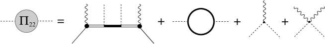
Figure 8: The term $A_{2}\Pi_{22}A_{2}$ according to Eq. (47). The first diagram on the right-hand side corresponds to the term $A_{2}\Pi_{\cal B}A_{2}$. The second diagram is the fermion-loop contribution to $A_{2}\Pi_{\rm loop}A_{2}$; there is an analogous one from a ghost loop. The last two diagrams correspond to $A_{2}\Pi_{\cal V}A_{2}$.

Figure 9: The term $A_{2}\Pi_{{\cal B}}A_{2}$.

Figure 10: The fermionic contribution to the term $A_{2}\Pi_{\rm loop}A_{2}$.

Figure 11: The term $A_{2}\Pi_{{\cal V}}A_{2}$.

The third term in Eq. (43) is quadratic in $A_{2}$, where

$$\Delta_{22}^{-1}[A_{1},\bar{\Psi}_{1},\Psi_{1}]\equiv-\left.\frac{\delta^{2}S[A,\bar{\Psi}_{1},\Psi_{1}]}{\delta A_{2}\,\delta A_{2}}\right|_{A_{2}=0}\equiv\Delta_{0,22}^{-1}+\Pi_{22}[A_{1},\bar{\Psi}_{1},\Psi_{1}]\,\,.$$ (46)

Here, $\Delta_{0,22}^{-1}$ is the free inverse propagator for hard gluons. Similar to the “current” ${\cal J}$, cf. Eq. (44), the “self-energy” $\Pi_{22}$ of hard gluons consists of three different contributions,

$$\Pi_{22}[A_{1},\bar{\Psi}_{1},\Psi_{1}]=\Pi_{{\cal B}}[A_{1},\bar{\Psi}_{1},\Psi_{1}]+\Pi_{\rm loop}[A_{1}]+\Pi_{{\cal V}}[A_{1}]\;,$$ (47)

which has a diagrammatic representation as shown in Fig. 8. The first two contributions on the right-hand side of Eq. (47) can be expanded as shown in Figs. 9 and 10. Figure 11 depicts the three- and four-gluon vertices contained in the last term in Eq. (47). For further use, we explicitly give the first term,

$$\Pi_{{\cal B}}[A_{1},\bar{\Psi}_{1},\Psi_{1}]=-\frac{1}{2}\,\bar{\Psi}_{1}\,\left(g\,\frac{\delta^{2}{\cal B}}{\delta A_{2}\delta A_{2}}\right)_{A_{2}=0}\Psi_{1}\;.$$ (48)

Finally, we collect all terms with more than two hard gluon fields $A_{2}$ in Eq. (43) in the “interaction action” for hard gluons, $S_{I}[A_{1},A_{2},\bar{\Psi}_{1},\Psi_{1}]$. We then perform the functional integration over the hard gluon fields $A_{2}$. Since functional integrals must be of Gaussian type in order to be exactly solvable, we resort to a method well-known from perturbation theory. We add the source term $A_{2}J_{2}$ to the action (37b) and may then replace the fields $A_{2}$ in $S_{I}$ by functional differentiation with respect to $J_{2}$, at $J_{2}=0$. We then move the factor $\exp\{S_{I}[A_{1},\delta/\delta J_{2},\bar{\Psi}_{1},\Psi_{1}]\}$ in front of the functional $A_{2}$-integral. Then, this functional integral is Gaussian and can be readily performed (after a suitable shift of $A_{2}$), with the result

$${\cal Z} = \int{\cal D}\bar{\Psi}_{1}\,{\cal D}\Psi_{1}{\cal D}A_{1}\,\exp\left\{S[A_{1},\bar{\Psi}_{1},\Psi_{1}]-\frac{1}{2}\,{\rm Tr}_{g}\ln\Delta_{22}^{-1}\right\}$$ (49)

$$\times\left.\exp\left\{S_{I}\left[A_{1},\frac{\delta}{\delta J_{2}},\bar{\Psi}_{1},\Psi_{1}\right]\right\}\,\exp\left[\frac{1}{2}\,({\cal J}+J_{2})\,\Delta_{22}\,({\cal J}+J_{2})\right]\right|_{J_{2}=0}\;.$$

The trace over $\ln\Delta_{22}^{-1}$ runs over gluon 4-momenta, as well as adjoint color and Lorentz indices. We indicate this with a subscript “$g$”. Note that this result is still exact and completely general, since so far our manipulations of the partition function were independent of the specific choice (42) for the projection operators ${\cal Q}_{1,2}$. The next step is to derive the tree-level action for the effective theory of relevant quark modes and soft gluons.

II.4 Tree-level effective action

In order to derive the tree-level effective action, we shall employ two approximations. The first is based on the principle assumption in the construction of any effective theory, namely that soft and hard modes are well separated in momentum space. Consequently, momentum conservation does not allow a hard gluon to couple to any (finite) number of soft gluons. Under this assumption, the diagrams generated by $A_{2}({\cal J}_{\rm loop}+{\cal J}_{{\cal V}})$, cf. Fig. 6, 7, will not occur in the effective theory. In the following, we shall therefore omit these terms, so that ${\cal J}\equiv{\cal J}_{{\cal B}}$. Note that similar arguments cannot be applied to the diagrams generated by $A_{2}(\Pi_{\rm loop}+\Pi_{{\cal V}})A_{2}$, cf. Fig. 10, 11, since now there are two hard gluon legs which take care of momentum conservation.

Our second approximation is that in the “perturbative” expansion of the partition function (49) with respect to powers of the interaction action $S_{I}$, we only take the first term, i.e., we approximate $e^{S_{I}}\simeq 1$. This is analogous to the derivation of the exact renormalization group in Ref. Wegner , where it was shown that the corresponding diagrams are of higher order and can be neglected. In our case, diagrams generated by $e^{S_{I}}$ are those with more than one resummed hard gluon line. Even with the approximation $e^{S_{I}}\simeq 1$, Eq. (49) still contains diagrams with arbitrarily many bare hard gluon lines, arising from the expansion of

$$\ln\Delta_{22}^{-1}=\ln\Delta_{0,22}^{-1}-\sum_{n=1}^{\infty}\frac{(-1)^{n}}{n}\,\left(\Delta_{0,22}\,\Pi_{22}\right)^{n}\;,$$ (50)

and from the term ${\cal J}_{{\cal B}}\Delta_{22}{\cal J}_{{\cal B}}$ in Eq. (49), when expanding

$$\Delta_{22}=\Delta_{0,22}\sum_{n=0}^{\infty}(-1)^{n}\left(\Pi_{22}\,\Delta_{0,22}\right)^{n}\;.$$ (51)

With these approximations, the partition function reads

$${\cal Z}=\int{\cal D}\bar{\Psi}_{1}\,{\cal D}\Psi_{1}{\cal D}A_{1}\,\exp\{S_{\rm eff}[A_{1},\bar{\Psi}_{1},\Psi_{1}]\}\;,$$ (52)

where the effective action is defined as

$$S_{\rm eff}[A_{1},\bar{\Psi}_{1},\Psi_{1}] \equiv S_{A}[A_{1}]+\frac{1}{2}\,\bar{\Psi}_{1}\left\{{\cal G}_{0,11}^{-1}+g{\cal B}[A_{1}]\right\}\Psi_{1}+\frac{1}{2}\,{\rm Tr}_{q}\ln{\cal G}_{22}^{-1}[A_{1}]-\frac{1}{2}\,{\rm Tr}_{g}\ln\Delta_{22}^{-1}[A_{1},\bar{\Psi}_{1},\Psi_{1}]$$ (53)

$$+\;\frac{1}{2}\,{\cal J}_{{\cal B}}[A_{1},\bar{\Psi}_{1},\Psi_{1}]\,\Delta_{22}[A_{1},\bar{\Psi}_{1},\Psi_{1}]\,{\cal J}_{{\cal B}}[A_{1},\bar{\Psi}_{1},\Psi_{1}]\;.$$

This is the desired action for the effective theory describing the interaction of relevant quark modes, $\bar{\Psi}_{1},\Psi_{1}$, and soft gluons, $A_{1}$. The functional dependence of the various terms on the right-hand side on the fields $A_{1},\bar{\Psi}_{1},\Psi_{1}$ has been restored in order to facilitate the following discussion of all possible interaction vertices occurring in this effective theory.

Figure 12: The three- and four-gluon vertices in $S_{A}[A_{1}]$, describing the self-interaction of soft gluons in Eq. (53).

Figure 13: The term $\bar{\Psi}_{1}\,g{\cal B}[A_{1}]\,\Psi_{1}$ in the effective action (53).

Figure 14: The term ${\rm Tr}_{q}\ln{\cal G}_{22}^{-1}[A_{1}]$ in the effective action (53).

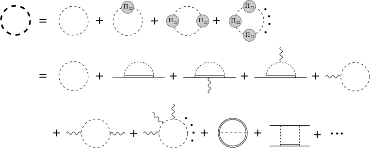
Figure 15: The term ${\rm Tr}_{g}\ln\Delta_{22}^{-1}[A_{1},\bar{\Psi}_{1},\Psi_{1}]$ in the effective action (53). The first line corresponds to the generic expansion (50), with “self-energy” insertions $\Pi_{22}$, as shown in Fig. 8. The second line contains some examples for diagrams generated when explicitly inserting the expression for $\Pi_{22}$.

Figure 16: The term ${\cal J}_{\cal B}\Delta_{22}{\cal J}_{\cal B}$ in the effective action (53). The thick dashed line is a full hard gluon propagator, i.e., it has the expansion (50). The first diagram on the right-hand side of this figure results from the $n=0$ term of this expansion, while the next three diagrams originate from the $n=1$ term. Even a single insertion of a hard gluon “self-energy” $\Pi_{22}$ gives rise to a variety of diagrams. Here, we only show the contributions corresponding to the first diagrams in Figs. 9, 10, and the three-gluon vertex. The last diagram arises from the second term of the expansion shown in Fig. 2.

The diagrams corresponding to these vertices are shown in Figs. 12-16. The three- and four-gluon vertices contained in $S_{A}[A_{1}]$ are displayed in Fig. 12. In addition, $S_{A}[A_{1}]$ contains ghost loops with an arbitrary number of attached soft gluon legs. The topology is equivalent to that of the quark loops in Fig. 14 and is therefore not shown explicitly. The interaction between two relevant quarks and the “modified” soft gluon field, corresponding to $\bar{\Psi}_{1}\,g{\cal B}[A_{1}]\,\Psi_{1}$, is depicted in Fig. 13. This is similar to Fig. 3, except that now all gluon legs are soft. Diagrams where an arbitrary number of soft gluon legs is attached to an irrelevant quark loop are generated by ${\rm Tr}_{q}\ln{\cal G}_{22}^{-1}$, cf. Fig. 14. This is similar to Fig. 4, but now only soft gluon legs are attached to the fermion loop. The diagrams generated by the loop of a full hard gluon propagator, ${\rm Tr}_{g}\ln\Delta_{22}^{-1}$, are shown in Fig. 15. The first line in this figure features the generic expansion of this term according to Eq. (50), where the hard gluon “self-energy” insertion $\Pi_{22}$, cf. Eq. (47), is shown in Fig. 8. The second line shows examples of diagrams generated by explicitly inserting $\Pi_{22}$ in the generic expansion. Besides an arbitrary number of soft gluon legs, these diagrams also feature an arbitrary number of relevant quark legs. If there are only two relevant quark legs, but no soft gluon leg, one obtains the one-loop self-energy for relevant quarks, cf. the second diagram in the second line of Fig. 15. The next two diagrams are obtained by adding a soft gluon leg, resulting in vertex corrections for the bare vertex between relevant quarks and soft gluons. The first of these two diagrams arises from the $n=1$ term in Eq. (50), while the second originates from the $n=2$ term. Four relevant quark legs and no soft gluon leg give rise to the scattering of two relevant quarks via exchange of two hard gluons, contained in the $n=2$ term in Eq. (50), cf. the last diagram in Fig. 15. This diagram was also discussed in the context of the effective theory presented in Refs. hong ; hong2 , cf. discussion in Sec. III.2. Finally, the “current-current” interaction mediated by a full hard gluon propagator, ${\cal J}_{{\cal B}}\,\Delta_{22}\,{\cal J}_{{\cal B}}$, Fig. 16, contains also a multitude of quark-gluon vertices. The simplest one is the first on the right-hand side in Fig. 16, corresponding to scattering of two relevant fermions via exchange of a single hard gluon.

The effective action (53) is formally of the form (7). The difference is that Eq. (53) contains more than one relevant field: besides relevant quarks there are also soft gluons. It is obvious that in this case there are many more possibilities to construct operators ${\cal O}_{i}$ which occur in the expansion (7). As pointed out in the introduction, it is therefore advantageous to derive the effective action (53) by explicitly integrating out irrelevant quark and hard gluon modes, and not by simply guessing the form of the operators ${\cal O}_{i}$, since then one is certain that one has constructed all possible operators occurring in the expansion (7).

As mentioned in the introduction, the standard approach to derive an effective theory, namely guessing the form of the operators ${\cal O}_{i}$ and performing a naive dimensional scaling analysis to estimate their order of magnitude, fails precisely when (a) there are non-local operators, or when (b) there is more than one momentum scale. Both (a) and (b) apply here. As we shall show below, the HTL/HDL effective action is one limiting case of Eq. (53), and it is well known that this action is non-local. Moreover, as is obvious from the above derivation, there are indeed several momentum scales occurring in Eq. (53). Let us focus on the case of zero temperature, $T=0$, and, for the sake of simplicity, assume massless quarks, $m=0$, $\mu=k_{F}$. To be explicit, we employ the choice (25) for the projectors ${\cal P}_{1,2}$. In this case, the first momentum scale is defined by the Fermi energy $\mu$. The propagator of antiquarks is $\sim 1/(k_{0}+\mu+k)$. If $\Lambda_{q},\Lambda_{g}\lesssim\mu$, the exchange of an antiquark can be approximated by a contact interaction with strength $\sim 1/\mu$, on the scale of the relevant quarks, $L_{q}\gg 1/\Lambda_{q}\gtrsim 1/\mu$, or of the soft gluons, $L_{g}\gg 1/\Lambda_{g}\gtrsim 1/\mu$.

The second momentum scale is defined by the quark cut-off momentum $\Lambda_{q}$. The propagator of irrelevant quark modes is $\sim 1/(k_{0}+\mu-k)$. On the scale $L_{q}$ of the relevant quarks, not only the exchange of an antiquark, but also that of an irrelevant quark with momentum ${\bf k}$ satisfying $|k-\mu|\geq\Lambda_{q}$ is local, with strength $\sim 1/\Lambda_{q}$. However, suppose that the quark cut-off scale happens to be much smaller than the chemical potential, $\Lambda_{q}\ll\mu$. In this case, antiquark exchange is “much more localized” than the exchange of an irrelevant quark, $1/\mu\ll 1/\Lambda_{q}$.

The third momentum scale is defined by the gluon cut-off momentum $\Lambda_{g}$. The propagator of a hard gluon is $\sim 1/P^{2}$. On the scale $L_{g}$ of a soft gluon, the exchange of a hard gluon with momentum $p\geq\Lambda_{g}$ can be considered local, with strength $\sim 1/\Lambda_{g}^{2}$. As we shall show below, in order to derive the value of the QCD gap parameter in weak coupling and to subleading order, the ordering of the scales turns out to be $\Lambda_{q}\lesssim g\mu\ll\Lambda_{g}\lesssim\mu$. Thus, antiquark exchange happens on a length scale of the same order as hard gluon exchange, which in turn happens on a much smaller length scale than the exchange of an irrelevant quark, $1/\mu\lesssim 1/\Lambda_{g}\ll 1/\Lambda_{q}$.

III Examples of effective theories

In this section we show that, for particular choices of the projectors ${\cal P}_{1,2}$ in Eq. (24), several well-known, at first sight unrelated effective theories for hot and/or dense quark matter, are in fact nothing but special cases of the general effective theory defined by the action (53). These are the HTL/HDL effective action for quarks and gluons, and the high-density effective theory for cold, dense quark matter.

III.1 HTL/HDL effective action

Let us first focus on the HTL/HDL effective action. This action defines an effective theory for massless quarks and gluons with small momenta in a system at high temperature $T$ (HTL), or large chemical potential $\mu$ (HDL). Consequently, the projectors ${\cal P}_{1,2}$ for quarks are given by

$${\cal P}_{1}(K,Q) = \Theta(\Lambda_{q}-k)\,\delta^{(4)}_{K,Q}\;,$$ (54a)

$${\cal P}_{2}(K,Q) = \Theta(k-\Lambda_{q})\,\delta^{(4)}_{K,Q}\;,$$ (54b)

while the projectors for gluons are given by Eq. (42). (We note that, strictly speaking, the quarks and gluons of the HTL/HDL effective action should also have small energies in real time. Since our effective action is defined in imaginary time, one should constrain the energy only at the end of a calculation, after analytically continuing the result to Minkowski space.)

The essential assumption to derive the HTL/HDL effective action is that there is a single momentum scale, $\Lambda_{q}=\Lambda_{g}\equiv\Lambda$, which separates hard modes with momenta $\sim T$, or $\sim\mu$, from soft modes with momenta $\sim gT$, or $\sim g\mu$. In the presence of an additional energy scale $T$, or $\mu$, naive perturbation theory in terms of powers of the coupling constant fails. It was shown by Braaten and Pisarski braatenpisarski that, for the $n$-gluon scattering amplitude the one-loop term, where $n$ soft gluon legs are attached to a quark or gluon loop, is as important as the tree-level diagram. The same holds for the scattering of $n-2$ gluons and 2 quarks. At high $T$ and small $\mu$, the momenta of the quarks and gluons in the loop are of the order of the hard scale, $\sim T$. This gives rise to the name “Hard Thermal Loop” effective action, and allows to simplify the calculation of the respective diagrams. At large $\mu$ and small $T$, i.e., for the HDL effective action, the situation is somewhat more involved. As gluons do not have a Fermi surface, the only physical scale which determines the order of magnitude of a loop consisting exclusively of gluon propagators is the temperature. Therefore, at small $T$ and large $\mu$, such pure gluon loops are negligible. On the other hand, the momenta of quarks in the loop are $\sim\mu$. Thus, only loops with at least one quark line need to be considered in the HDL effective action.

In order to show that the HTL/HDL effective action is contained in the effective action (53), we first note that a soft particle cannot become hard by interacting with another soft particle. This has the consequence that a soft quark cannot turn into a hard one by soft-gluon scattering. Therefore,

$$g{\cal B}[A_{1}]\equiv g{\cal A}_{11}\;.$$ (55)

Another consequence is that the last term in Eq. (53), ${\cal J}_{{\cal B}}\Delta_{22}{\cal J}_{{\cal B}}$, vanishes since ${\cal J}_{{\cal B}}$ is identical to a vertex between a soft quark and a hard gluon, which is kinematically forbidden. The resulting action then reads

$$S_{\mbox{\scriptsize large}\,T/\mu}[A_{1},\bar{\Psi}_{1},\Psi_{1}]\equiv S_{A}[A_{1}]+\frac{1}{2}\,\bar{\Psi}_{1}\left({\cal G}_{0,11}^{-1}+g{\cal A}_{11}\right)\Psi_{1}+\frac{1}{2}\,{\rm Tr}_{q}\ln{\cal G}_{22}^{-1}[A_{1}]-\frac{1}{2}\,{\rm Tr}_{g}\ln\Delta_{22}^{-1}[A_{1},\bar{\Psi}_{1},\Psi_{1}]\;.$$ (56)

Using the expansion (36) we realize that the term ${\rm Tr}_{q}\ln{\cal G}_{22}^{-1}$ generates all one-loop diagrams, where $n$ soft gluon legs are attached to a hard quark loop. This is precisely the quark-loop contribution to the HTL/HDL effective action.

For hard gluons with momentum $\sim T$ or $\sim\mu$, the free inverse gluon propagator is $\Delta_{0,22}^{-1}\sim T^{2}$ or $\sim\mu^{2}$, while the contribution $\Pi_{\rm loop}$ to the hard gluon “self-energy” (47) is at most of the order $\sim g^{2}T^{2}$ or $\sim g^{2}\mu^{2}$. Consequently, $\Pi_{\rm loop}$ can be neglected and $\Pi_{22}$ only contains tree-level diagrams, $\Pi_{22}\equiv\Pi_{{\cal B}}+\Pi_{{\cal V}}$. Using the expansion (50) of ${\rm Tr}_{g}\ln\Delta_{22}^{-1}$, the terms which contain only insertions of $\Pi_{{\cal V}}$ correspond to one-loop diagrams where $n$ soft gluon legs are attached to a hard gluon loop. As was shown in Ref. braatenpisarski , with the exception of the two-gluon amplitude, the loops with four-gluon vertices are suppressed. Neglecting these, we are precisely left with the pure gluon loop contribution to the HTL effective action. As discussed above, for the HDL effective action, this contribution is negligible.

The “self-energy” $\Pi_{{\cal B}}$ contains only two soft quark legs attached to a hard quark propagator (via emission and absorption of hard gluons). Consequently, in the expansion (50) of ${\rm Tr}_{g}\ln\Delta_{22}^{-1}$, the terms which contain insertions of $\Pi_{{\cal V}}$ and $\Pi_{{\cal B}}$ correspond to one-loop diagrams where an arbitrary number of soft quark and gluon legs is attached to the loop. It was shown in Ref. braatenpisarski that of these diagrams, only the ones with two soft quark legs and no four-gluon vertices are kinematically important and thus contribute to the HTL/HDL effective action. We have thus shown that this effective action, $S_{\rm HTL/HDL}$, is contained in the effective action (56), and constitutes its leading contribution,

$$S_{\mbox{\scriptsize large}\,T/\mu}=S_{\rm HTL/HDL}+\,\mbox{higher orders}\;.$$ (57)

For the sake of completeness, let us briefly comment on possible ghost contributions. Ghost loops arise from the term ${\rm Tr}_{gh}\ln{\cal W}^{-1}$ in $S_{A}[A_{1}]$. Their topology and consequently their properties are completely analogous to those of the pure gluon loops discussed above.

We conclude with a remark regarding the HDL effective action. According to Eq. (54), at zero temperature and large chemical potential, a soft quark or antiquark has a momentum $k\sim g\mu$, i.e., it lies at the bottom of the Fermi sea, or at the top of the Dirac sea, respectively. These modes are, however, not that important in degenerate Fermi systems, because it requires a large amount of energy $k_{0}\sim\mu$ to excite them. The truly relevant modes are quark modes with large momenta, $k\sim\mu$, close to the Fermi surface, because it costs little energy to excite them. A physically reasonable effective theory for cold, dense quark matter should therefore feature no antiquark modes at all, and only quark modes near the Fermi surface. Such a theory will be discussed in the following.

III.2 High-density effective theory

An effective theory for high-density quark matter was first proposed by Hong hong and was further refined by Schäfer and others HLSLHDET ; schaferefftheory ; NFL ; others . In the construction of this effective theory, one first proceeds similar to our discussion in Sec. II and integrates out antiquark modes. (From a technical point of view, this is not done as in Sec. II by functional integration, but by employing the equations of motion for antiquarks. The result is equivalent.) On the other hand, at first all quark modes in the Fermi sea are considered as relevant. Consequently, in the notation of Sec. II, the choice for the projectors ${\cal P}_{1,2}$ would be

$${\cal P}_{1}(K,Q) = \left(\begin{array}[]{cc}\Lambda_{\bf k}^{+}&0\\ 0&\Lambda_{\bf k}^{-}\end{array}\right)\,\delta^{(4)}_{K,Q}\;,$$ (58c)

$${\cal P}_{2}(K,Q) = \left(\begin{array}[]{cc}\Lambda_{\bf k}^{-}&0\\ 0&\Lambda_{\bf k}^{+}\end{array}\right)\,\delta^{(4)}_{K,Q}\;.$$ (58f)

Also, at first gluons are not separated into soft and hard modes either. After this step, the partition function of the theory assumes the form (8) with ${\cal Z}_{q}$ given by Eq. (31).

In the next step, one departs from the rigorous approach of integrating out modes, as done in Sec. II, and follows the standard way of constructing an effective theory, as explained in the introduction. One focusses exclusively on quark modes close to the Fermi surface as well as on soft gluons. However, since quark modes far from the Fermi surface and hard gluons are not explicitly integrated out, the effective action does not automatically contain the terms which reflect the influence of these modes on the relevant quark and soft gluon degrees of freedom. Instead, the corresponding terms have to be written down “by hand” and the effective vertices have to be determined via matching to the underlying microscopic theory, i.e., QCD.

In order to further organize the terms occurring in the effective action, one covers the Fermi surface with “patches”. Each patch is labelled according to the local Fermi velocity, ${\bf v}_{F}\equiv\hat{\bf k}\,k_{F}/\mu$ at its center. A patch is supposed to have a typical size $\Lambda_{\parallel}$ in radial ($\hat{\bf k}$) direction, and a size $\Lambda_{\perp}$ tangential to the Fermi surface. The momentum of quark modes inside a patch is decomposed into a large component in the direction of ${\bf v}_{F}$, the particular Fermi velocity labelling the patch under consideration, and a small residual component, ${\bf l}$, residing exclusively inside the patch,

$${\bf k}=\mu\,{\bf v}_{F}+{\bf l}\;.$$ (59)

The residual component is further decomposed into a component pointing in radial direction, ${\bf l}_{\parallel}\equiv{\bf v}_{F}({\bf v}_{F}\cdot{\bf l})$, and the orthogonal one, tangential to the Fermi surface, ${\bf l}_{\perp}\equiv{\bf l}-{\bf l}_{\parallel}$. The actual covering of the Fermi surface with such patches is not unique. One should, however, make sure that neighbouring patches do not overlap, in order to avoid double-counting of modes near the Fermi surface. In this case, the total number of patches on the Fermi surface is $\sim\mu^{2}/\Lambda_{\perp}^{2}$.

In the following, we shall show that the action of the high-density effective theory as discussed in Refs. hong ; hong2 ; HLSLHDET ; schaferefftheory ; NFL ; others is contained in our effective action (53). To this end, however, we shall employ the choice (25) and (42) for the projectors for quark and gluon modes, and not Eq. (58) for the quark projectors. As in Refs. hong ; hong2 ; HLSLHDET ; schaferefftheory ; NFL ; others , the quark mass will be set to zero, $m=0$. We also have to clarify how the patches covering the Fermi surfaces introduced in Refs. hong ; hong2 ; HLSLHDET ; schaferefftheory ; NFL ; others arise within our effective theory. It is obvious that the radial dimension $\Lambda_{\parallel}$ of a patch is related to the quark cut-off $\Lambda_{q}$. We simply choose $\Lambda_{\parallel}\equiv\Lambda_{q}$. Similarly, since soft-gluon exchange is not supposed to move a fermion from a particular patch to another, the dimension $\Lambda_{\perp}$ tangential to the Fermi surface must be related to the gluon cut-off $\Lambda_{g}$. Again, we adhere to the most simple choice $\Lambda_{\perp}\equiv\Lambda_{g}$. Since $\Lambda_{g}\lesssim\mu$, this is consistent with the matching procedure discussed in Ref. HLSLHDET , where the matching scale is chosen as $\Lambda_{\perp}=\sqrt{2}\mu$ (which is only slightly larger than $\mu$). The different scales $\Lambda_{q},\,\Lambda_{g}$, and $\mu$ are illustrated in Fig. 17. The modulus of the residual momentum ${\bf l}$ in Eq. (59) is constrained to $l\leq{\rm max}\,(\Lambda_{q},\,\Lambda_{g})$.

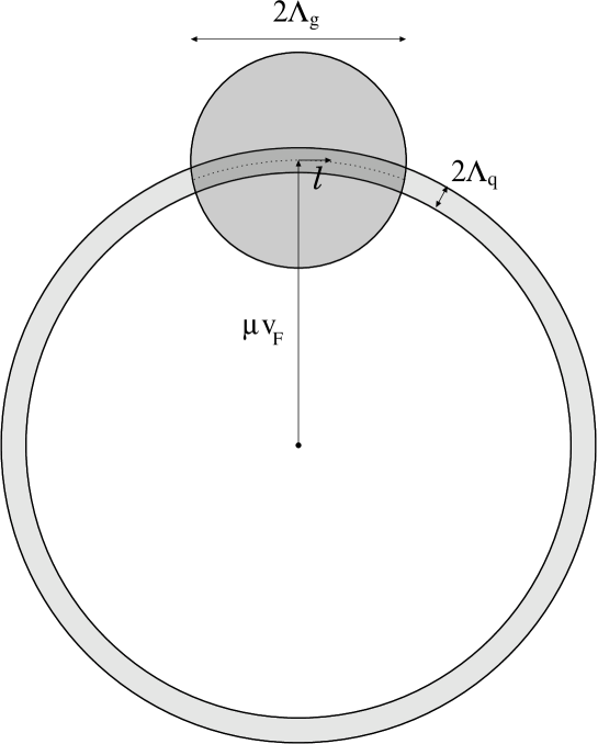
Figure 17: A particular patch covering the Fermi surface. The tangential dimension, $\Lambda_{\perp}$, is given by the maximum momentum transferred via a soft gluon, $\Lambda_{g}$, while the radial dimension, $\Lambda_{\parallel}$ is defined by the maximum distance of relevant quark modes from the Fermi surface, $\Lambda_{q}$. Also shown is a typical momentum transfer ${\bf l}$ via a soft gluon.

In Nambu-Gor’kov space, the leading, kinetic term in the Lagrangian of the high-density effective theory reads

$${\cal L}_{\rm kin}=\frac{1}{2}\,\sum_{{\bf v}_{F}}\bar{\Psi}_{1}(X,{\bf v}_{F})\gamma_{0}\,\left(\begin{array}[]{cc}iV\cdot D&0\\ 0&i\bar{V}\cdot D_{C}\end{array}\right)\,\Psi_{1}(X,{\bf v}_{F})\;,$$ (60)

cf. for instance Eq. (1) of Ref. schaferefftheory . Here, we have introduced the 4-vectors

$$V^{\mu}\equiv(1,{\bf v}_{F})\;\;\;\;,\;\;\;\;\;\bar{V}^{\mu}\equiv(1,-{\bf v}_{F})\;.$$ (61)

The covariant derivative for charge-conjugate fields is defined as $D^{\mu}_{C}\equiv\partial^{\mu}+igA^{\mu}_{a}T_{a}^{T}$. The contribution (60) arises from the term $\bar{\Psi}_{1}\,\left({\cal G}_{0,11}^{-1}\,+g{\cal A}_{11}\right)\,\Psi_{1}$ in Eq. (53). In order to see this, use ${\cal P}_{1}^{2}\equiv{\cal P}_{1}$ to write

$$\frac{1}{2}\,\bar{\Psi}_{1}\,{\cal G}_{0,11}^{-1}\,\Psi_{1} = \frac{1}{2}\,\bar{\Psi}_{1}\,\gamma_{0}{\cal P}_{1}\gamma_{0}\,{\cal G}_{0,11}^{-1}\,{\cal P}_{1}\,\Psi_{1}$$ (64)

$$= \frac{1}{2}\sum_{K,Q}\bar{\Psi}_{1}(K)\gamma_{0}\,\frac{1}{T}\,\left(\begin{array}[]{cc}k_{0}+\mu-k&0\\ 0&k_{0}-\mu+k\end{array}\right)\,\delta^{(4)}_{K,Q}\,\Psi_{1}(Q)$$

$$\simeq \frac{1}{2}\sum_{{\bf v}_{F},L}\bar{\Psi}_{1}(L,{\bf v}_{F})\gamma_{0}\,\frac{1}{T}\,\left(\begin{array}[]{cc}V\cdot L&0\\ 0&\bar{V}\cdot L\end{array}\right)\,\Psi_{1}(L,{\bf v}_{F})\;.$$ (67)

In the last step, we have approximated $k\simeq\mu+{\bf v}_{F}\cdot{\bf l}$, which holds up to terms of order $O(l^{2}/\mu)$, cf. Eq. (59). This is a good approximation if the modulus of a typical residual quark momentum in the effective theory is $l\ll{\rm max}\,(\Lambda_{q},\,\Lambda_{g})\lesssim\mu$. We have also introduced the 4-vector $L^{\mu}\equiv(k_{0},{\bf l})$ and, applying the decomposition (59), we have written the sum over ${\bf k}$ as a double sum over ${\bf v}_{F}$ and ${\bf l}$. The latter sum runs over all residual momenta ${\bf l}$ inside a given patch, while the former runs over all patches. With this decomposition, the spinors $\bar{\Psi}_{1}$, $\Psi_{1}$ are defined locally on a given patch (labelled by the Fermi velocity ${\bf v}_{F}$), and depend on the 4-momentum $L$. Note that a Fourier transformation to coordinate space converts $V\cdot L\rightarrow iV\cdot\partial$.

Now consider the term $\bar{\Psi}_{1}g{\cal A}_{11}\Psi_{1}$. Since ${\cal A}_{11}$ is not diagonal in momentum space, cf. Eq. (23), in principle the two quark spinors $\bar{\Psi}_{1}$, $\Psi_{1}$ can belong to different patches. However, we have chosen the tangential dimension of a patch such that a (typical) soft gluon can by definition never move a fermion across the border of a particular patch, $|{\bf k}-{\bf q}|\ll\Lambda_{g}$. Therefore, both spinors reside in the same patch and, to leading order, $\hat{\bf k}\simeq\hat{\bf q}\simeq{\bf v}_{F}$. With these assumptions we may write $\Lambda_{\bf k}^{-}A\hbox to0.0pt{\hss/\kern 0.0pt}_{a}(K-Q)\Lambda_{\bf q}^{+}\simeq V\cdot A_{a}(K-Q)\,\gamma_{0}\,\Lambda^{+}_{\bf k}$, $\Lambda_{\bf k}^{+}A\hbox to0.0pt{\hss/\kern 0.0pt}_{a}(K-Q)\Lambda_{\bf q}^{-}\simeq\bar{V}\cdot A_{a}(K-Q)\,\gamma_{0}\,\Lambda^{-}_{\bf k}$. Then, introducing the residual momentum ${\bf l}^{\prime}$ corresponding to the quark 3-momentum ${\bf q}$ and defining ${L^{\prime}}^{\mu}\equiv(q_{0},{\bf l}^{\prime})$, the respective term in the effective action becomes

$$\frac{1}{2}\,\bar{\Psi}_{1}\,g{\cal A}_{11}\,\Psi_{1}\simeq\frac{1}{2}\,\frac{g}{\sqrt{VT^{3}}}\sum_{{\bf v}_{F},L,L^{\prime}}\bar{\Psi}_{1}(L,{\bf v}_{F})\gamma_{0}\,\left(\begin{array}[]{cc}V\cdot A_{a}(L-L^{\prime})\,T_{a}&0\\ 0&-\bar{V}\cdot A_{a}(L-L^{\prime})\,T_{a}^{T}\end{array}\right)\,\Psi_{1}(L^{\prime},{\bf v}_{F})\;.$$ (68)

In coordinate space, the sum of Eqs. (67) and (68) becomes Eq. (60).

Subleading terms of order $O(1/\mu)$ in the high-density effective theory are of the form

$${\cal L}_{O(1/\mu)}=-\frac{1}{2}\sum_{{\bf v}_{F}}\bar{\Psi}_{1}(X,{\bf v}_{F})\gamma_{0}\,\frac{1}{2\mu}\left(\begin{array}[]{cc}D_{\perp}^{2}-\frac{g}{2}\,\sigma^{\mu\nu}F_{\perp\mu\nu}^{a}T_{a}&0\\ 0&-D_{C\perp}^{2}-\frac{g}{2}\,\sigma^{\mu\nu}F_{\perp\mu\nu}^{a}T_{a}^{T}\end{array}\right)\Psi_{1}(X,{\bf v}_{F})\;,$$ (69)

cf. Eq. (2) of Ref. schaferefftheory . Here, $D_{\perp}^{\mu}\equiv\{0,({\bf 1}-{\bf v}_{F}{\bf v}_{F})\cdot{\bf D}\}$, and similarly for $D_{C\perp}^{\mu}$. The commutator of two gamma matrices is defined as usual, $\sigma^{\mu\nu}\equiv(i/2)[\gamma^{\mu},\gamma^{\nu}]$, and $F_{\perp\mu\nu}^{a}T_{a}\equiv(i/g)[D_{\perp\mu},D_{\perp\nu}]$. As we shall see in the following, this contribution arises from the term $-g^{2}\,\bar{\Psi}_{1}\,{\cal A}_{12}\,{\cal G}_{22}\,{\cal A}_{21}\,\Psi_{1}$ in Eq. (53).

First, note that, with the projectors (25), the irrelevant quark propagator ${\cal G}_{22}$ contains quark as well as antiquark modes. In order to derive Eq. (69), however, we have to discard the quark and keep only the antiquark modes. In essence, this is a consequence of the simpler choice (58) for the projectors ${\cal P}_{1,2}$ in the high-density effective theory of Refs. hong ; hong2 ; HLSLHDET ; schaferefftheory ; NFL ; others . In this case, the propagator ${\cal G}_{22}$ may be simplified. A calculation quite similar to that of Eqs. (67) and (68) now leads (in coordinate space) to

$${\cal G}_{22}^{-1}\equiv{\cal G}_{0,22}^{-1}+g{\cal A}_{22}\simeq\gamma_{0}\,\tau_{3}\left(\begin{array}[]{cc}2\mu+i\bar{V}\cdot D&0\\ 0&2\mu-iV\cdot D_{C}\end{array}\right)\;,$$ (70)

where $\tau_{3}$ acts in Nambu-Gor’kov space. This result may be readily inverted to yield

$${\cal G}_{22}\simeq\gamma_{0}\,\tau_{3}\,\frac{1}{2\mu}\sum_{n=0}^{\infty}\frac{1}{(2\mu)^{n}}\left(\begin{array}[]{cc}-i\bar{V}\cdot D&0\\ 0&iV\cdot D_{C}\end{array}\right)^{n}\;.$$ (71)

Utilizing the projectors (58), one may also derive a simpler form for $g{\cal A}_{12}$ and $g{\cal A}_{21}$. Consider, for instance, the term $\bar{\Psi}_{1}\,g{\cal A}_{12}\,\Psi_{2}$. We follow the same steps that led to Eqs. (67), i.e., we assume that the spinors $\bar{\Psi}_{1}$ and $\Psi_{2}$ reside in the same patch, such that $\hat{\bf k}\simeq\hat{\bf q}\simeq{\bf v}_{F}$. This allows to derive the identity $\Lambda_{\bf k}^{\mp}\,A\hbox to0.0pt{\hss/\kern 0.0pt}^{a}(K-Q)\Lambda_{\bf q}^{\mp}\simeq\Lambda_{\bf k}^{\mp}A\hbox to0.0pt{\hss/\kern 0.0pt}^{a}_{\perp}(K-Q)$, where $A_{\perp}^{\mu a}\equiv\{0,({\bf 1}-{\bf v}_{F}{\bf v}_{F})\cdot{\bf A}^{a}\}$. Now introduce the 4-vectors $L^{\mu}$, ${L^{\prime}}^{\mu}$, as in Eq. (68), which leads to

$$\frac{1}{2}\,\bar{\Psi}_{1}\,g{\cal A}_{12}\,\Psi_{2}\simeq\frac{1}{2}\,\frac{g}{\sqrt{VT^{3}}}\sum_{{\bf v}_{F},L,L^{\prime}}\bar{\Psi}_{1}(L,{\bf v}_{F})\left(\begin{array}[]{cc}A\hbox to0.0pt{\hss/\kern 0.0pt}^{a}_{\perp}(L-L^{\prime})\,T_{a}&0\\ 0&-A\hbox to0.0pt{\hss/\kern 0.0pt}^{a}_{\perp}(L-L^{\prime})\,T_{a}^{T}\end{array}\right)\Psi_{2}(L^{\prime},{\bf v}_{F})\;.$$ (72)

We may add a term $L\hbox to0.0pt{\hss/\kern 0.0pt}_{\perp}$ to the diagonal Nambu-Gor’kov components, which trivially vanishes between spinors $\bar{\Psi}_{1}$ and $\Psi_{2}$. This has the advantage that, in coordinate space,

$$g{\cal A}_{12}\simeq\left(\begin{array}[]{cc}iD\hbox to0.0pt{\hss/\kern 1.0pt}_{\perp}&0\\ 0&iD\hbox to0.0pt{\hss/\kern 1.0pt}_{C\perp}\end{array}\right)\;,$$ (73)

i.e., this term transforms covariantly under gauge transformations, and no longer as a gauge field. A similar calculation for $g{\cal A}_{21}$ gives the result $g{\cal A}_{21}\equiv g{\cal A}_{12}$. Combining Eqs. (71) and (73), the term $-g^{2}\,\bar{\Psi}_{1}\,{\cal A}_{12}\,{\cal G}_{22}\,{\cal A}_{21}\,\Psi_{1}$ corresponds to the following contribution in the Lagrangian,

$$-\frac{1}{2}\sum_{{\bf v}_{F}}\bar{\Psi}_{1}(X,{\bf v}_{F})\gamma_{0}\left(\begin{array}[]{cc}D\hbox to0.0pt{\hss/\kern 1.0pt}_{\perp}&0\\ 0&-D\hbox to0.0pt{\hss/\kern 1.0pt}_{C\perp}\end{array}\right)\frac{1}{2\mu}\sum_{n=0}^{\infty}\frac{1}{(2\mu)^{n}}\left(\begin{array}[]{cc}-i\bar{V}\cdot D&0\\ 0&iV\cdot D_{C}\end{array}\right)^{n}\left(\begin{array}[]{cc}D\hbox to0.0pt{\hss/\kern 1.0pt}_{\perp}&0\\ 0&D\hbox to0.0pt{\hss/\kern 1.0pt}_{C\perp}\end{array}\right)\Psi_{1}(X,{\bf v}_{F})\;.$$ (74)

Taking only the $n=0$ term, and utilizing $\gamma^{\mu}\gamma^{\nu}\equiv g^{\mu\nu}-i\sigma^{\mu\nu}$, one arrives at Eq. (69). Note that our definition for transverse quantities, e.g. $A_{\perp}^{\mu}\equiv\{0,({\bf 1}-{\bf v}_{F}{\bf v}_{F})\cdot{\bf A}\}$, slightly differs from that of Refs. hong ; hong2 , where $A_{\perp}^{\mu}\equiv A^{\mu}-V^{\mu}V\cdot A$. However, both definitions agree when sandwiched between spinors $\bar{\Psi}_{1,2}$ and $\Psi_{2,1}$.

At order $O(1/\mu^{2})$, besides the $n=1$ term in Eq. (74), there are also four-fermion interaction terms, cf. Eqs. (3-5) of Ref. schaferefftheory . In the effective action (53), these contributions arise from the term ${\cal J}_{{\cal B}}\Delta_{22}{\cal J}_{{\cal B}}$ which originates from integrating out hard gluons. (Since this is not done explicitly in the construction of the high-density effective theory in Refs. hong ; hong2 ; HLSLHDET ; schaferefftheory ; NFL ; others , this term is not automatically generated, but has to be added “by hand”.) To leading order, this term corresponds to the exchange of a hard gluon between two quarks, cf. the first diagram on the right-hand side of Fig. 16. If the quarks are close to the Fermi surface, the energy in the hard gluon propagator can be neglected, and $\Delta_{0,22}\lesssim 1/\Lambda_{g}^{2}$. Since $1/\Lambda_{g}^{2}\gtrsim 1/\mu^{2}$, the contribution from hard-gluon exchange is of order $O(1/\mu^{2})$. Four-fermion interactions also receive corrections at one-loop order, cf. Fig. 5 of Ref. hong2 . In Eq. (53), they are contained in the term ${\rm Tr}\ln\Delta_{22}^{-1}$, see the last diagram in Fig. 15.

Besides the quark terms in the Lagrangian of the high-density effective theory hong ; hong2 ; HLSLHDET ; schaferefftheory ; NFL ; others , there are also contributions from gluons. The first is the standard Yang-Mills Lagrangian $-(1/4)F_{\mu\nu}^{a}F^{\mu\nu}_{a}$, cf. Eq. (1) of Ref. schaferefftheory . This part is contained in the term $S_{A}[A_{1}]$ in Eq. (53), cf. Eq. (9). The second contribution is a mass term for magnetic gluons,

$${\cal L}_{m_{g}}=-\frac{m_{g}^{2}}{2}\,{\bf A}^{a}\cdot{\bf A}^{a}\;,$$ (75)

cf. Eq. (19) of Ref. SonStephanov , Eq. (18) of Ref. hong2 , or Eq. (27) of Ref. HLSLHDET , where $m_{g}$ is the gluon mass parameter (6). This term has to be added “by hand” in order to obtain the correct value for the HDL gluon polarization tensor within the high-density effective theory. In Eq. (53) this contribution arises from the $n=2$ term of the expansion (36) of ${\rm Tr}\ln{\cal G}_{22}^{-1}$. The gluon polarization tensor has contributions from particle-hole and particle-antiparticle excitations. The latter give rise to ${\cal L}_{m_{g}}$. While this term arises naturally within our derivation of the effective theory, it does not in the high-density effective theory of Refs. hong ; hong2 ; HLSLHDET ; schaferefftheory ; NFL ; others , because only antiquarks, but not irrelevant quark modes, are explicitly integrated out. Irrelevant quark modes can then only be taken into account by adding the appropriate counter terms.

Sometimes, the full HDL action is added to the Lagrangian of the high-density effective theory, cf. Eq. (8) of Ref. schaferefftheory . This procedure requires a word of caution. For instance, an important contribution to the HDL polarization tensor arises from particle-hole excitations around the Fermi surface. Such excitations are still relevant degrees of freedom in the effective theory. However, in order for them to appear in the gluon polarization tensor they would first have to be integrated out. Therefore, strictly speaking such contributions cannot occur in the tree-level effective action. Of course, in an effective theory one is free to add whatever contributions one deems necessary. However, one has to be careful to avoid double counting. As will be shown in Sec. IV, the full HDL polarization tensor will appear quite naturally in an approximate solution to the Schwinger-Dyson equation for the gluon propagator, however, not at tree-, but only at (one-)loop level.

It was claimed in Refs. hong2 ; HLSLHDET ; schaferefftheory that a consistent power-counting scheme within the high-density effective theory requires $\Lambda_{\perp}=\Lambda_{\parallel}$. In contrast, we shall show in Sec. IV that a computation of the gap parameter to subleading order requires $\Lambda_{q}\equiv\Lambda_{\parallel}\ll\Lambda_{\perp}\equiv\Lambda_{g}$. This means that irrelevant quark modes become local on a scale $l_{q}\gg 1/\Lambda_{q}$, while antiquark modes become local already on a much smaller scale, $l_{\bar{q}}\gg 1/\mu$, cf. discussion at the end of Sec. II. As mentioned in the introduction, for two different scales power counting of terms in the effective action becomes a non-trivial problem. While the high-density effective theory of Refs. hong ; hong2 ; HLSLHDET ; schaferefftheory ; NFL ; others contains effects from integrating out antiquarks, i.e., from the scale $1/\mu$, the effective action (53) in addition keeps track of the influence of irrelevant quark modes, i.e., from physics on the scale $1/\Lambda_{q}\gg 1/\mu$. Since all terms in the effective action (53) are kept, one can be certain not to miss any important contribution just because the naive dimensional power-counting scheme is invalidated by the occurrence of two vastly different length scales.

IV Calculation of the QCD gap parameter

In this section, we demonstrate how the effective theory derived in Sec. II can be applied to compute the gap parameter of color-superconducting quark matter to subleading order. For the sake of definiteness, we shall consider a spin-zero, two-flavor color superconductor.

IV.1 CJT formalism for the effective theory

The gap parameter in superconducting systems is not accessible by means of perturbation theory; one has to apply non-perturbative, self-consistent, many-body resummation techniques to calculate it. For this purpose, it is convenient to employ the CJT formalism CJT . The first step is to add source terms to the effective action (53),

$$S_{\rm eff}[A_{1},\bar{\Psi}_{1},\Psi_{1}]\;\longrightarrow\;S_{\rm eff}[A_{1},\bar{\Psi}_{1},\Psi_{1}]+J_{1}A_{1}+\frac{1}{2}\,A_{1}K_{1}A_{1}+\frac{1}{2}\left(\bar{\Psi}_{1}H_{1}+\bar{H}_{1}\Psi_{1}+\bar{\Psi}_{1}{\cal K}_{1}\Psi_{1}\right)\;,$$ (76)

where we employed the compact matrix notation defined in Eq. (22). $J_{1}$, $\bar{H}_{1}$, and $H_{1}$ are local source terms for the soft gluon and relevant quark fields, respectively, while $K_{1}$ and ${\cal K}_{1}$ are bilocal source terms. The bilocal source ${\cal K}_{1}$ for quarks is also a matrix in Nambu-Gor’kov space. Its diagonal components are source terms which couple quarks to antiquarks, while its off-diagonal components couple quarks to quarks. The latter have to be introduced for systems which can become superconducting, i.e., where the ground state has a non-vanishing diquark expectation value, $\langle\psi_{1}\psi_{1}\rangle\neq 0$.

One then performs a Legendre transformation with respect to all sources and arrives at the CJT effective action CJT ; kleinert

$$\Gamma\left[A,\bar{\Psi},\Psi,\Delta,{\cal G}\right] = S_{\rm eff}\left[A,\bar{\Psi},\Psi\right]-\frac{1}{2}\,{\rm Tr}_{g}\ln\Delta^{-1}-\frac{1}{2}\,{\rm Tr}_{g}\left(D^{-1}\Delta-1\right)$$ (77)

$$+ \frac{1}{2}\,{\rm Tr}_{q}\ln{\cal G}^{-1}+\frac{1}{2}\,{\rm Tr}_{q}\left(G^{-1}{\cal G}-1\right)+\Gamma_{2}\left[A,\bar{\Psi},\Psi,\Delta,{\cal G}\right]\;.$$

Here, $S_{\rm eff}[A,\bar{\Psi},\Psi]$ is the tree-level action defined in Eq. (53), which now depends on the expectation values $A\equiv\langle A_{1}\rangle$, $\bar{\Psi}\equiv\langle\bar{\Psi}_{1}\rangle$, and $\Psi\equiv\langle\Psi_{1}\rangle$ for the one-point functions of soft gluon and relevant quark fields. In a slight abuse of notation, we use the same symbols for the expectation values as for the original fields, prior to integrating out modes. This should not lead to confusion, as the original fields no longer occur in any of the following expressions.

The quantities $D^{-1}$ and $G^{-1}$ in Eq. (77) are the inverse tree-level propagators for soft gluons and relevant quarks, respectively, which are determined from the effective action $S_{\rm eff}$, see below. The quantities $\Delta$ and ${\cal G}$ are the expectation values for the two-point functions, i.e., the full propagators, of soft gluons and relevant quarks. The functional $\Gamma_{2}$ is the sum of all two-particle irreducible (2PI) diagrams. These diagrams are vacuum diagrams, i.e., they have no external legs. They are constructed from the vertices defined by the interaction part of $S_{\rm eff}$, linked by full propagators $\Delta$, ${\cal G}$. The expectation values for the one- and two-point functions of the theory are determined from the stationarity conditions

$$0=\frac{\delta\Gamma}{\delta A}=\frac{\delta\Gamma}{\delta\bar{\Psi}}=\frac{\delta\Gamma}{\delta\Psi}=\frac{\delta\Gamma}{\delta\Delta}=\frac{\delta\Gamma}{\delta{\cal G}}\;.$$ (78)

The first condition yields the Yang-Mills equation for the expectation value $A$ of the soft gluon field. The second and third condition correspond to the Dirac equation for $\Psi$ and $\bar{\Psi}$, respectively. The effective action (53) contains a multitude of terms which depend on $A,\bar{\Psi},\Psi$, and thus the Yang-Mills and Dirac equations are rather complex, wherefore we refrain from explicitly presenting them here. Nevertheless, for the Dirac equation the solution is trivial, since $\bar{\Psi}_{1},\,\Psi_{1}$ are Grassmann-valued fields, and their expectation values must vanish identically, $\bar{\Psi}=\langle\bar{\Psi}_{1}\rangle=\Psi=\langle\Psi_{1}\rangle\equiv 0$. On the other hand, for the Yang-Mills equation, the solution $A$ is in general non-zero but, at least for the two-flavor color superconductor considered here, it was shown Gerhold ; DirkDennis to be parametrically small, $A\sim\phi^{2}/(g^{2}\mu)$, where $\phi$ is the color-superconducting gap parameter. Therefore, to subleading order in the gap equation it can be neglected.

The fourth and fifth condition (78) are Dyson-Schwinger equations for the soft gluon and relevant quark propagator, respectively,

$$\Delta^{-1} = D^{-1}+\Pi\;,$$ (79a)

$${\cal G}^{-1} = G^{-1}+\Sigma\;,$$ (79b)

where

$$\Pi \equiv -2\,\frac{\delta\Gamma_{2}}{\delta\Delta^{T}}\;,$$ (80a)

$$\Sigma \equiv 2\,\frac{\delta\Gamma_{2}}{\delta{\cal G}^{T}}$$ (80b)

are the gluon and quark self-energies, respectively. The Dyson-Schwinger equation for the relevant quark propagator is a $2\times 2$ matrix equation in Nambu-Gor’kov space,

$${\cal G}^{-1}=\left(\begin{array}[]{cc}[G^{+}]^{-1}&0\\ 0&[G^{-}]^{-1}\end{array}\right)+\left(\begin{array}[]{cc}\Sigma^{+}&\Phi^{-}\\ \Phi^{+}&\Sigma^{-}\end{array}\right)\;,$$ (81)

where $\Sigma^{+}$ is the regular self-energy for quarks and $\Sigma^{-}$ the corresponding one for charge-conjugate quarks. The off-diagonal self-energies $\Phi^{\pm}$, the so-called gap matrices, connect regular with charge-conjugate quark degrees of freedom. A non-zero $\Phi^{\pm}$ corresponds to the condensation of quark Cooper pairs. Only two of the four components of this matrix equation are independent, say $[G^{+}]^{-1}+\Sigma^{+}$ and $\Phi^{+}$, the other two can be obtained via $[G^{-}]^{-1}+\Sigma^{-}=C\{[G^{+}]^{-1}+\Sigma^{+}\}^{T}C^{-1}$, $\Phi^{-}\equiv\gamma_{0}[\Phi^{+}]^{\dagger}\gamma_{0}$. Equation (81) can be formally solved for ${\cal G}$ manuel2 ,

$${\cal G}\equiv\left(\begin{array}[]{cc}{\cal G}^{+}&\Xi^{-}\\ \Xi^{+}&{\cal G}^{-}\end{array}\right)\;,$$ (82)

where

$${\cal G}^{\pm}\equiv\left\{[G^{\pm}]^{-1}+\Sigma^{\pm}-\Phi^{\mp}\left([G^{\mp}]^{-1}+\Sigma^{\mp}\right)^{-1}\Phi^{\pm}\right\}^{-1}$$ (83)

is the propagator describing normal propagation of quasiparticles and their charge-conjugate counterpart, while

$$\Xi^{\pm}\equiv-\left([G^{\mp}]^{-1}+\Sigma^{\mp}\right)^{-1}\Phi^{\pm}{\cal G}^{\pm}$$ (84)

describes anomalous propagation of quasiparticles, which is possible if the ground state is a color-superconducting quark-quark condensate, for details, see Ref. DHRreview .

The tree-level gluon propagator is defined as

$$D^{-1}\equiv-\frac{\delta^{2}S_{\rm eff}[A,\bar{\Psi},\Psi]}{\delta A\,\delta A}\;.$$ (85)

Since we ultimately evaluate the tree-level propagator at the stationary point of $\Gamma$, Eq. (78), where $\bar{\Psi}=\Psi=0$, we may omit all terms in $S_{\rm eff}$, Eq. (53), which are proportional to the quark fields. The only terms which contribute to the tree-level gluon propagator are therefore

$$D^{-1}\equiv-\frac{\delta^{2}}{\delta A\,\delta A}\left(S_{A}+\frac{1}{2}\,{\rm Tr}_{q}\ln{\cal G}_{22}^{-1}-\frac{1}{2}\,{\rm Tr}_{g}\ln\Delta_{22}^{-1}\right)\;.$$ (86)

Using the expansions (34), (36), (50), and (51), and exploiting the cyclic property of the trace, one finds

$$D^{-1}=-\frac{\delta^{2}S_{A}}{\delta A\,\delta A}-\frac{g}{2}\,{\rm Tr}_{q}\left(\frac{\delta{\cal G}_{22}}{\delta A}\,\frac{\delta{\cal A}_{22}}{\delta A}\right)+\frac{1}{2}{\rm Tr}_{g}\left(\frac{\delta\Delta_{22}}{\delta A}\,\frac{\delta\Pi_{22}}{\delta A}+\Delta_{22}\,\frac{\delta^{2}\Pi_{22}}{\delta A\,\delta A}\right)\;.$$ (87)

In order to proceed, note that the Dyson-Schwinger equations (79) are evaluated at the stationary point of the effective action, where $\bar{\Psi}=\Psi=0,\,A\simeq 0$. For $A=0$, the first term yields the free inverse propagator for soft gluons, $\Delta_{0,11}^{-1}$, cf. Eq. (38), plus a contribution from the Faddeev-Popov determinant, $(\delta^{2}{\rm Tr}_{gh}\ln{\cal W}^{-1}/\delta A\delta A)_{A=0}$. The contributions from the three- and four-gluon vertex vanish for $A=0$. Furthermore, according to Eq. (23),

$$\frac{\delta{\cal A}_{22}(K,Q)}{\delta A(P)}=\frac{1}{\sqrt{VT^{3}}}\,\hat{\Gamma}\,\delta^{(4)}_{K,Q+P}\equiv\tilde{\Gamma}(K,Q;P)\;.$$ (88)

This is a matrix in fundamental color, flavor, and Nambu-Gor’kov space, as well as in the space of quark 4-momenta $K,Q$. It is a vector in Minkowski and adjoint color space ($\hat{\Gamma}$ carries a Lorentz-vector and a gluon color index), as well as in the space of gluon 4-momenta $P$. We evaluate $(\delta{\cal G}_{22}/\delta A)_{A=0}$ using the expansion (34). Only the term for $n=1$ survives when taking $A=0$. For $\bar{\Psi}=\Psi=0$, we have $\Pi_{\cal B}=0$, cf. Fig. 9, and we only need to consider $\Pi_{22}=\Pi_{\rm loop}+\Pi_{{\cal V}}$. Then, the term ${\cal V}^{(3)}\equiv(\delta\Pi_{{\cal V}}/\delta A)_{A=0}$ corresponds to a triple-gluon vertex, cf. Fig. 11, where two hard gluons couple to one soft gluon. The term $(\delta\Pi_{\rm loop}/\delta A)_{A=0}$ is a correction to this vertex: it couples two hard gluons to a soft one through an (irrelevant) quark loop, cf. Fig. 10. According to arguments well-known from the HTL/HDL effective theory, this vertex correction can never be of the same order as the tree-level vertex ${\cal V}^{(3)}$, since the two incoming gluons are hard. We therefore neglect $(\delta\Pi_{\rm loop}/\delta A)_{A=0}$ in the following. Similarly, ${\cal V}^{(4)}\equiv(\delta^{2}\Pi_{{\cal V}}/\delta A\delta A)_{A=0}$ is a four-gluon vertex, cf. Fig. 11, where two hard gluons couple to two soft ones, and $(\delta^{2}\Pi_{\rm loop}/\delta A\delta A)_{A=0}$ is the one-(quark-)loop correction to this vertex, cf. Fig. 10. Applying the same arguments as above, we only keep ${\cal V}^{(4)}$. Arguments from the HTL/HDL effective theory also tell us that to leading order we may approximate $\Delta_{22}\simeq\Delta_{0,22}$. Finally, utilizing the same arguments we approximate $\delta\Delta_{22}/\delta A\simeq-\Delta_{0,22}{\cal V}^{(3)}\Delta_{0,22}$. Then, the inverse tree-level gluon propagator of Eq. (87) becomes

$$D^{-1}=\Delta_{0,11}^{-1}+\frac{g^{2}}{2}\,{\rm Tr}_{q}\left({\cal G}_{0,22}\,\tilde{\Gamma}\,{\cal G}_{0,22}\,\tilde{\Gamma}\right)-\frac{1}{2}\,{\rm Tr}_{g}\left(\Delta_{0,22}\,{\cal V}^{(3)}\,\Delta_{0,22}\,{\cal V}^{(3)}\right)+\frac{1}{2}\,{\rm Tr}_{g}\left(\Delta_{0,22}\,{\cal V}^{(4)}\right)-\left.\frac{\delta^{2}{\rm Tr}_{gh}\ln{\cal W}^{-1}}{\delta A\,\delta A}\right|_{A=0}\;.$$ (89)

The second term represents an (irrelevant) quark-loop, while the third term is a hard gluon loop. The fourth term is a hard gluon tadpole. Finally, the last term in Eq. (89) corresponds to a ghost loop necessary to cancel loop contributions from unphysical gluon degrees of freedom. Note that, in the effective theory, loop contributions involving irrelevant quarks and hard gluons occur already in the tree-level action (53). Therefore, such loops also arise in the inverse tree-level propagator (89) for the soft gluons of the effective theory. For the projection operators (42) and (54) the inverse tree-level propagator (89) is precisely the HTL/HDL-resummed inverse gluon propagator. For small temperatures, $T\ll\mu$, the contribution from the gluon and ghost loops is negligible as compared to that from the quark loop,

$$D^{-1}\simeq\Delta_{0,11}^{-1}+\frac{g^{2}}{2}\,{\rm Tr}_{q}\left({\cal G}_{0,22}\,\tilde{\Gamma}\,{\cal G}_{0,22}\,\tilde{\Gamma}\right)\;.$$ (90)

The inverse tree-level quark propagator is defined as

$$G^{-1}\equiv-2\,\frac{\delta^{2}S_{\rm eff}[A,\bar{\Psi},\Psi]}{\delta\bar{\Psi}\,\delta{\Psi}}\;.$$ (91)

For $\bar{\Psi}=\Psi=0$, the last term in Eq. (53) does not contribute to $G^{-1}$, because it has at least four external quark legs, and the two functional derivatives $\delta/\delta\bar{\Psi}$, $\delta/\delta\Psi$ amputate only two of them. The first and the third term in Eq. (53) do not depend on $\bar{\Psi},\Psi$ at all, therefore

$$G^{-1}={\cal G}_{0,11}^{-1}+g{\cal B}[A]+\frac{\delta^{2}{\rm Tr}_{g}\ln\Delta_{22}^{-1}}{\delta\bar{\Psi}\,\delta\Psi}\;.$$ (92)

Using the expansion formulae (50) and (51) and the fact that $\Pi_{22}$ depends on $\bar{\Psi},\Psi$ only through $\Pi_{\cal B}$, we obtain

$$\frac{\delta^{2}{\rm Tr}_{g}\ln\Delta_{22}^{-1}}{\delta\bar{\Psi}\,\delta{\Psi}}={\rm Tr}_{g}\left(\Delta_{22}\frac{\delta^{2}\Pi_{{\cal B}}}{\delta\bar{\Psi}\,\delta{\Psi}}\right)\;.$$ (93)

We have exploited the fact that this expression is evaluated at $\bar{\Psi}=\Psi=0$, i.e., terms with external quark legs will eventually vanish. The trace runs only over adjoint colors, Lorentz indices, and (hard) gluon 4-momenta. Since $\Delta_{22}$ is a hard gluon propagator, the contribution from $\Pi_{22}$ to $\Delta_{22}$ may be neglected to the order we are computing, and we may set $\Delta_{22}\simeq\Delta_{0,22}$. Furthermore, $(\delta^{2}\Pi_{{\cal B}}/\delta\bar{\Psi}\delta\Psi)_{A=0}\equiv-g^{2}\,\tilde{\Gamma}\,{\cal G}_{0,22}\,\tilde{\Gamma}$, cf. Fig. 9. At $\bar{\Psi}=\Psi=0,\,A\simeq 0$ we are left with

$$G^{-1}={\cal G}_{0,11}^{-1}-g^{2}\,{\rm Tr}_{g}\left(\Delta_{0,22}\,\tilde{\Gamma}\,{\cal G}_{0,22}\,\tilde{\Gamma}\right)\;.$$ (94)

As was the case for the tree-level gluon propagator, also the tree-level quark propagator receives a loop contribution; here it arises from a loop involving an irrelevant quark and a hard gluon line. The term $\tilde{\Gamma}{\cal G}_{0,22}\tilde{\Gamma}$ under the gluon trace remains a matrix in the quark indices, i.e., fundamental color, flavor, Dirac, and quark 4-momenta.

We now proceed to solve the Dyson-Schwinger equations (79) for the soft gluon and relevant quark propagator. To this end, we have to determine $\Gamma_{2}$. Of course, it is not feasible to consider all possible 2PI diagrams. The advantage of the CJT formalism is that any truncation of $\Gamma_{2}$ defines a meaningful, self-consistent many-body approximation for which one can solve the Dyson-Schwinger equations (79). In our truncation of $\Gamma_{2}$ we only take into account 2-loop diagrams which are 2PI with respect to the soft gluon and relevant quark propagators $\Delta,\,{\cal G}$,

$$\Gamma_{2}=-\frac{g^{2}}{4}\,{\rm Tr}_{q,g}\left({\cal G}\,\tilde{\Gamma}\,{\cal G}\,\tilde{\Gamma}\,\Delta\right)-\frac{g^{2}}{2}\,{\rm Tr}_{q,g}\left({\cal G}\,\tilde{\Gamma}\,{\cal G}_{0,22}\,\tilde{\Gamma}\,\Delta\right)-\frac{g^{2}}{4}\,{\rm Tr}_{q,g}\left({\cal G}\,\tilde{\Gamma}\,{\cal G}\,\tilde{\Gamma}\,\Delta_{0,22}\right)\;.$$ (95)

The traces now run over quark as well as over gluon indices. Consider, for instance, the term ${\cal G}\,\tilde{\Gamma}\,{\cal G}\,\tilde{\Gamma}$. It is a matrix in the space of fundamental color, flavor, Dirac and quark 4-momenta, of which the trace is taken through ${\rm Tr}_{q}$. In addition, due to the two factors $\tilde{\Gamma}$ it carries two Lorentz-vector, adjoint-color, and gluon-4-momenta indices. The trace ${\rm Tr}_{g}$ contracts these indices with the corresponding ones from the gluon propagator $\Delta$.

Figure 18: Diagrammatic representation of $\Gamma_{2}$, Eq. (95).

The diagrams corresponding to Eq. (95) are shown in Fig. 18. The first two terms are constructed from the quark-gluon coupling $\sim\bar{\Psi}\,g{\cal B}\,\Psi$. Using Eq. (33), one may either obtain an ordinary quark-gluon vertex $\sim g\,\bar{\Psi}\,{\cal A}\,\Psi$, involving one soft gluon and two relevant quark legs, or a vertex $\sim g^{2}\,\bar{\Psi}\,{\cal A}\,{\cal G}_{22}\,{\cal A}\,\Psi$, with (at least) two soft gluon legs and two relevant quark legs. To lowest order, we approximate ${\cal G}_{22}\simeq{\cal G}_{0,22}$, which neglects vertices with more than two soft gluon legs. Taking two ordinary quark-gluon vertices and tying them together to obtain a 2PI 2-loop diagram, we arrive at the first term in Eq. (95), or the first diagram in Fig. 18. Taking one of the two-gluon-two-quark vertices and tying the legs together, one obtains the second term in Eq. (95), or the second diagram in Fig. 18, respectively. Finally, the third term/diagram arises from the last term in Eq. (53). To lowest order, this corresponds to a four-quark vertex $\sim g^{2}\,\bar{\Psi}\,\tilde{\Gamma}\,\Psi\,\Delta_{0,22}\bar{\Psi}\,\tilde{\Gamma}\,\Psi$. Tying the quark legs together to form a 2PI diagram, one obtains the corresponding term/diagram in Eq. (95)/Fig. 18.

The combinatorial factors in front of the various terms in Eq. (95) are explained as follows. In the first diagram, there are two ordinary quark-gluon vertices. According to Eq. (53), each comes with a factor 1/2. Moreover, since there are two vertices, the diagram is, in the perturbative sense, a diagram of second order, which causes an additional factor 1/2 FTFT . Finally, there are two possibilities to connect the quark lines between the two vertices. In total, we then have a prefactor $-(1/2)^{2}\times 1/2\times 2=-1/4$, where the minus sign arises from the fermion loop. The second diagram arises from the two-quark-two-gluon vertex, which already comes with a prefactor $-1/2$ in Eq. (53). It is perturbatively of first order, and there is only one possibility to tie the quark and gluon lines together, so there is no additional combinatorial factor (and no additional minus sign) for this diagram. Finally, the third diagram arises from the four-quark vertex, $(1/2){\cal J}_{{\cal B}}\Delta_{0,22}{\cal J}_{{\cal B}}$, in Eq. (53). This vertex comes with a factor 1/2 and is perturbatively of first order. However, there are two additional factors 1/2 residing in ${\cal J}_{{\cal B}}$, since ${\cal J}_{{\cal B}}\sim(1/2)\bar{\Psi}\,\hat{\Gamma}\,\Psi$, cf. Eq. (45). Again, there are two possibilities to tie the quark lines together, so that, in total, we have a prefactor $-1/2\times(1/2)^{2}\times 2=-1/4$, where the minus sign again stands for the quark loop.

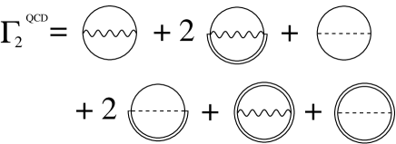
Figure 19: Diagrammatic representation of $\Gamma_{2}^{\rm QCD}$, after decomposing quark lines into relevant and irrelevant, as well as gluon propagators into soft and hard contributions.

At this point, it is instructive to compare $\Gamma_{2}$, Eq. (95), in the effective theory with $\Gamma_{2}^{\rm QCD}$ which one would have written down in QCD at the same loop level. $\Gamma_{2}^{\rm QCD}$ would be equivalent to the first diagram of Fig. 18, but now the quark and gluon lines represent the full propagators for all momentum modes, relevant and irrelevant as well as soft and hard. In order to compare with $\Gamma_{2}$ of the effective theory, we decompose the quark propagators into relevant and irrelevant modes, and the gluon propagator into soft and hard modes. One obtains the six diagrams shown in Fig. 19. The first three are precisely the same that occur in $\Gamma_{2}$ of the effective theory, including the combinatorial prefactors. The last three diagrams do not occur in $\Gamma_{2}$ of the effective theory, because they are not 2PI with respect to the relevant quark propagator ${\cal G}$ and the soft gluon propagator $\Delta$. Nevertheless, they are still included in the CJT effective action of the effective theory, Eq. (77): opening the relevant quark line of the fourth diagram, we recognize the loop contribution to the tree-level quark propagator $G^{-1}$, cf. Eq. (94). Now consider the fifth term in Eq. (77): here, this loop contribution to $G^{-1}$ is multiplied with ${\cal G}$ and traced over, which yields the fourth diagram in $\Gamma_{2}^{\rm QCD}$. Similarly, opening the soft gluon line of the fifth diagram, we identify this diagram as the irrelevant quark-loop contribution to the tree-level gluon propagator $D^{-1}$, cf. Eq. (90). The third term in Eq. (77), where this contribution is multiplied by $\Delta$ and traced over, then yields the fifth diagram of $\Gamma_{2}^{\rm QCD}$. Finally, the sixth diagram resides in the term $\sim{\rm Tr}_{g}\ln\Delta_{22}^{-1}$ of the tree-level effective action $S_{\rm eff}$, cf. Fig. 15. Therefore, in principle, the CJT effective action (77) for the effective theory contains the same information as the corresponding one for QCD. However, while in QCD self-consistency is maintained for all momentum modes via the solution of the stationarity condition (78), in the effective theory self-consistency is only required for the relevant quark and soft gluon modes. In this sense, the effective theory provides a simplification of the full problem.

IV.2 Dyson-Schwinger equations for relevant quarks and soft gluons

After having specified $\Gamma_{2}$ in Eq. (95), we are now in the position to write down the Dyson-Schwinger equations (79) explicitly. For the full inverse propagator of soft gluons we obtain with Eqs. (79a), (80a), (90), and (95)

$$\Delta^{-1}=\Delta_{0,11}^{-1}+\frac{g^{2}}{2}\,\left[{\rm Tr}_{q}\left({\cal G}_{0,22}\,\tilde{\Gamma}\,{\cal G}_{0,22}\,\tilde{\Gamma}\right)+2\,{\rm Tr}_{q}\left({\cal G}\,\tilde{\Gamma}\,{\cal G}_{0,22}\,\tilde{\Gamma}\right)+{\rm Tr}_{q}\left({\cal G}\,\tilde{\Gamma}\,{\cal G}\,\tilde{\Gamma}\right)\right]\;.$$ (96)

The first term in square brackets takes into account the effect of quark-antiquark excitations as well as quark-hole excitations far from the Fermi surface. The second term is the contribution from excitations where one quark is close to the Fermi surface (a relevant quark) while the second is far from the Fermi surface or an antiquark (an irrelevant quark). The relevant quark propagator ${\cal G}$ can have diagonal elements in Nambu-Gor’kov space, corresponding to normal propagation of quasiparticles, as well as off-diagonal elements, corresponding to anomalous propagation of quasiparticles, cf. Eq. (82). However, in the second term in square brackets the latter contribution is absent, because ${\cal G}_{0,22}$ is purely diagonal in Nambu-Gor’kov space, cf. Eq. (19). This is different for the last term in square brackets, which corresponds to quark-hole excitations close to the Fermi surface. Both quark propagators have to be determined self-consistently and may have off-diagonal elements in Nambu-Gor’kov space. Consequently, the trace over Nambu-Gor’kov space gives two contributions, a loop where both quarks propagate normally, and another one where they propagate anomalously. Diagrams of this type have been evaluated in Ref. Meissner2f3f and lead to the Meissner effect for gluons in a color superconductor.

For the full inverse propagator of relevant quarks we obtain with Eqs. (79b), (80b), (94), and (95)

$${\cal G}^{-1}={\cal G}_{0,11}^{-1}-g^{2}\,\left[{\rm Tr}_{g}\left(\Delta_{0,22}\,\tilde{\Gamma}\,{\cal G}_{0,22}\,\tilde{\Gamma}\right)+{\rm Tr}_{g}\left(\Delta\,\tilde{\Gamma}\,{\cal G}_{0,22}\,\tilde{\Gamma}\right)+{\rm Tr}_{g}\left(\Delta_{0,22}\,\tilde{\Gamma}\,{\cal G}\,\tilde{\Gamma}\right)+{\rm Tr}_{g}\left(\Delta\,\tilde{\Gamma}\,{\cal G}\,\tilde{\Gamma}\right)\right]\;.$$ (97)

The first two terms in square brackets do not have off-diagonal components in Nambu-Gor’kov space. They contribute only to the regular quark self-energy. The other two terms in square brackets have both diagonal and off-diagonal components in Nambu-Gor’kov space. The diagonal components contribute to the regular quark self-energy, in particular, the fourth term leads to the quark wave-function renormalization factor computed first in Ref. manuel . It gives rise to non-Fermi liquid behavior rockefeller . The off-diagonal components enter the gap equation for the color-superconducting gap parameter.

The system of Eqs. (96) and (97) has to be solved self-consistently for the full propagators of quarks and gluons. However, as was shown in Ref. dirkselfenergy , in order to extract the color-superconducting gap parameter to subleading order it is sufficient to consider the gluon propagator in HDL approximation; corrections arising from the color-superconducting gap in the quasiparticle spectrum are of sub-subleading order in the gap equation. For our purpose this means that it is not necessary to self-consistently solve Eq. (96) together with Eq. (97); we may approximate ${\cal G}$ on the right-hand side of Eq. (96) by ${\cal G}_{0,11}$. In essence, this is equivalent to considering only the first term on the right-hand side of Eq. (97) when solving Eq. (96). Of course, under this approximation the effect of the regular quark self-energy (leading to wave-function renormalization) and of the anomalous quark self-energy (which accounts for the gap in the quasiparticle excitation spectrum) are neglected.

With this approximation, and using ${\cal G}_{0}\equiv{\cal G}_{0,11}\oplus{\cal G}_{0,22}$, we may combine the terms in Eq. (96) to give

$$\Delta^{-1}\simeq\Delta_{0,11}^{-1}+\frac{g^{2}}{2}\,{\rm Tr}_{q}\left({\cal G}_{0}\,\tilde{\Gamma}\,{\cal G}_{0}\,\tilde{\Gamma}\right)\;.$$ (98)

Taking the gluon cut-off scale $\Lambda_{g}$ to fulfill $g\mu\ll\Lambda_{g}\lesssim\mu$, soft gluons are defined to have momenta of order $g\mu$. We compute the fermion loop in Eq. (98) under this assumption (taking the soft gluon energy to be of the same order of magnitude as the gluon momentum). We then realize that the soft gluon propagator determined by Eq. (98) is just the gluon propagator in HDL approximation. We indicate this fact in the following by a subscript, $\Delta\equiv\Delta_{\rm HDL}$. Armed with this (approximate) solution of the Dyson-Schwinger equation (96) we now proceed to solve Eq. (97). We consider the two independent components $[G^{+}]^{-1}+\Sigma^{+}$ and $\Phi^{+}$ in Nambu-Gor’kov space separately. Due to translational invariance, it is convenient to define $[G^{+}]^{-1}(K,Q)\equiv(1/T)[G^{+}]^{-1}(K)\,\delta^{(4)}_{K,Q}$, $\Sigma^{+}(K,Q)\equiv(1/T)\Sigma^{+}(K)\,\delta^{(4)}_{K,Q}$, and using Eqs. (17), (19), (39), (88), we obtain the Dyson-Schwinger equation for $[G^{+}]^{-1}+\Sigma^{+}$,

$$[G^{+}]^{-1}(K)+\Sigma^{+}(K) = [G_{0,11}^{+}]^{-1}(K)$$ (99)

$$- g^{2}\,\frac{T}{V}\sum_{Q}\left\{\frac{}{}\left[\Delta_{0,22}\right]^{\mu\nu}_{ab}(K-Q)+\left[\Delta_{\rm HDL}\right]^{\mu\nu}_{ab}(K-Q)\right\}\gamma_{\mu}T^{a}\,G_{0,22}(Q)\,\gamma_{\nu}T^{b}$$

$$- g^{2}\,\frac{T}{V}\sum_{Q}\left\{\frac{}{}\left[\Delta_{0,22}\right]^{\mu\nu}_{ab}(K-Q)+\left[\Delta_{\rm HDL}\right]^{\mu\nu}_{ab}(K-Q)\right\}\gamma_{\mu}T^{a}\,{\cal G}^{+}(Q)\,\gamma_{\nu}T^{b}\;.$$

Note that the first sum over $Q$ runs over irrelevant quark momenta, $0\leq q<\mu-\Lambda_{q}$ and $\mu+\Lambda_{q}<q<\infty$, while the second sum runs over relevant quark momenta, $\mu-\Lambda_{q}\leq q\leq\mu+\Lambda_{q}$. There is no double counting of gluon exchange contributions, since the hard gluon propagator $\Delta_{0,22}$ has support only for gluon momenta $|{\bf k}-{\bf q}|>\Lambda_{g}$, while the HDL propagator is restricted to gluon momenta $|{\bf k}-{\bf q}|\leq\Lambda_{g}$. To subleading order in the gap equation, we do not have to solve this Dyson-Schwinger equation self-consistently. It is sufficient to use the approximation ${\cal G}^{+}\simeq G_{0,11}^{+}$ on the right-hand side of Eq. (99) and to keep only the last term which, as discussed above, is responsible for non-Fermi liquid behavior in cold, dense quark matter. The net result is then simply a wave-function renormalization for the free quark propagator $G_{0,11}^{+}$ manuel ,

$$[G^{+}]^{-1}(K)+\Sigma^{+}(K)\simeq[G_{0,11}^{+}]^{-1}(K)+\bar{g}^{2}\,k_{0}\,\gamma_{0}\,\ln\frac{M^{2}}{k_{0}^{2}}\equiv\left[Z^{-1}(k_{0})\,k_{0}+\mu\right]\,\gamma_{0}-\bm{\gamma}\cdot{\bf k}\;,$$ (100)

where $\bar{g}\equiv g/(3\sqrt{2}\pi)$ and $M^{2}=(3\pi/4)m_{g}^{2}$, with the gluon mass parameter $m_{g}$ defined in Eq. (6). Neglecting effects from the finite life-time of quasi-particles manuel2 , which are of sub-subleading order in the gap equation, the wave-function renormalization factor is

$$Z(k_{0})=\left(1+\bar{g}^{2}\,\ln\frac{M^{2}}{k_{0}^{2}}\right)^{-1}\;.$$ (101)

Due to translational invariance, it is convenient to define $\Phi^{+}(K,Q)\equiv(1/T)\,\Phi^{+}(K)\,\delta^{(4)}_{K,Q}$ and $\Xi^{+}(K,Q)\equiv T\,\Xi^{+}(K)\,\delta^{(4)}_{K,Q}$, and the Dyson-Schwinger equation for $\Phi^{+}(K)$ becomes

$$\Phi^{+}(K)=g^{2}\,\frac{T}{V}\sum_{Q}\left\{\frac{}{}\left[\Delta_{0,22}\right]^{\mu\nu}_{ab}(K-Q)+\left[\Delta_{\rm HDL}\right]^{\mu\nu}_{ab}(K-Q)\frac{}{}\right\}\,\gamma_{\mu}(T^{a})^{T}\,\Xi^{+}(Q)\,\gamma_{\nu}T^{b}\;.$$ (102)

Here, the sum runs only over relevant quark momenta, $\mu-\Lambda_{q}\leq q\leq\mu+\Lambda_{q}$. This is the gap equation for the color-superconducting gap parameter within our effective theory. There is no contribution from irrelevant fermions, since their propagator is diagonal in Nambu-Gor’kov space.

While the gluon cut-off was taken to be $\Lambda_{g}\lesssim\mu$, so that soft gluons have typical momenta of order $g\mu$, so far we have not specified the magnitude of $\Lambda_{q}$. In weak coupling, the color-superconducting gap function is strongly peaked around the Fermi surface son ; rdpdhr ; schaferwilczek . For a subleading-order calculation of the gap parameter, it is therefore sufficient to consider as relevant quark modes those within a thin layer of width $2\Lambda_{q}$ around the Fermi surface. For the following, our principal assumption is $\Lambda_{q}\lesssim g\mu\ll\Lambda_{g}\lesssim\mu$. As we shall see below, this assumption is crucial to identify sub-subleading corrections to the gap equation (102), which arise, for instance, from the pole of the gluon propagator. Note that this assumption is different from that of Refs. hong2 ; schaferefftheory , where it is assumed that $\Lambda_{q}\simeq\Lambda_{g}$.

For a two-flavor color superconductor, the color-flavor-spin structure of the gap matrix is DHRreview

$$\Phi^{+}(K)=J_{3}\tau_{2}\gamma_{5}\,\Lambda_{\bf k}^{+}\,\Theta(\Lambda_{q}-|k-\mu|)\,\phi(K)\;,$$ (103)

where $(J_{3})_{ij}\equiv-i\epsilon_{ij3}$ and $(\tau_{2})_{fg}\equiv-i\epsilon_{fg}$ represent the fact that quark pairs condense in the color-antitriplet, flavor-singlet channel. The Dirac matrix $\gamma_{5}$ restricts quark pairing to the even-parity channel (which is the preferred one due to the $U(1)_{A}$ anomaly of QCD). In the effective action (53), antiquark and irrelevant quark degrees of freedom are integrated out. The condensation of antiquark or irrelevant quark pairs, while in principle possible, is thus not taken into account; the bilocal source terms in Eq. (76) only allow for the condensation of relevant quark degrees of freedom. The condensation of antiquarks or irrelevant quarks could also be accounted for, if one introduces bilocal source terms already in Eq. (13), i.e., prior to integrating out any of the quark degrees of freedom. While there is in principle no obstacle in following this course of action, it is, however, not really necessary if one is interested in a calculation of the color-superconducting gap parameter to subleading order in weak coupling: antiquarks contribute to the gap equation beyond subleading order aqgap , and the gap function for quarks falls off rapidly away from the Fermi surface, i.e., in the region of irrelevant quark modes, and thus also contributes at most to sub-subleading order to the gap equation. Consequently, the Dirac structure of the gap matrix (102) contains only the projector $\Lambda_{\bf k}^{+}$ onto positive energy states. The theta function accounts for the fact that the gap function $\phi(K)$ pertains only to relevant quark modes.

Inserting Eq. (100) and the corresponding one for $[G^{-}]^{-1}+\Sigma^{-}$, as well as Eq. (103), into the definition (84) for the anomalous quark propagator, one obtains

$$\Xi^{+}(Q)=J_{3}\tau_{2}\gamma_{5}\,\Lambda_{\bf q}^{-}\,\Theta(\Lambda_{q}-|q-\mu|)\,\frac{\phi(Q)}{[q_{0}/Z(q_{0})]^{2}-\epsilon_{q}^{2}}\;.$$ (104)

One now plugs this expression into the gap equation (102), multiplies both sides with $J_{3}\tau_{2}\gamma_{5}\Lambda_{\bf k}^{+}$, and traces over color, flavor, and Dirac degrees of freedom. These traces simplify considerably since both hard and HDL gluon propagators are diagonal in adjoint color space, $[\Delta_{0,22}]^{\mu\nu}_{ab}\equiv\delta_{ab}\,\Delta_{0,22}^{\mu\nu}$, $[\Delta_{\rm HDL}]^{\mu\nu}_{ab}\equiv\delta_{ab}\,\Delta_{\rm HDL}^{\mu\nu}$. The result is an integral equation for the gap function $\phi(K)$,

$$\phi(K)=\frac{g^{2}}{3}\,\frac{T}{V}\sum_{Q}\left[\frac{}{}\Delta_{0,22}^{\mu\nu}(K-Q)+\Delta_{\rm HDL}^{\mu\nu}(K-Q)\frac{}{}\right]\,{\rm Tr}_{s}\left(\Lambda_{\bf k}^{+}\gamma_{\mu}\Lambda_{\bf q}^{-}\gamma_{\nu}\right)\,\frac{\phi(Q)}{[q_{0}/Z(q_{0})]^{2}-\epsilon_{q}^{2}}\;.$$ (105)

The sum over $Q$ runs only over relevant quark momenta, $|q-\mu|\leq\Lambda_{q}$. Also, the 3-momentum ${\bf k}$ is relevant, $|k-\mu|\leq\Lambda_{q}$.

IV.3 Solution of the gap equation

In pure Coulomb gauge, both the hard gluon and the HDL propagators have the form

$$\Delta^{00}(P)=\Delta^{\ell}(P)\;\;\;\;,\;\;\;\;\;\Delta^{0i}(P)=0\;\;\;\;,\;\;\;\;\;\Delta^{ij}(P)=(\delta^{ij}-\hat{p}^{i}\hat{p}^{j})\,\Delta^{t}(P)\;,$$ (106)

where $\Delta^{\ell,t}$ are the propagators for longitudinal and transverse gluon degrees of freedom. For hard gluons

$$\Delta^{\ell}_{0,22}(P) = -\frac{1}{p^{2}}\;,$$ (107a)

$$\Delta^{t}_{0,22}(P) = -\frac{1}{P^{2}}\;,$$ (107b)

while for soft, HDL-resummed gluons

$$\Delta^{\ell}_{\rm HDL}(P) = -\frac{1}{p^{2}-\Pi^{\ell}_{\rm HDL}(P)}\;,$$ (108a)

$$\Delta^{t}_{\rm HDL}(P) = -\frac{1}{P^{2}-\Pi^{t}_{\rm HDL}(P)}\;,$$ (108b)

with the HDL self-energies LeBellac

$$\Pi^{\ell}_{\rm HDL}(p_{0},p) = -3\,m_{g}^{2}\left[1-\frac{p_{0}}{2p}\,\ln\left(\frac{p_{0}+p}{p_{0}-p}\right)\right]\;,$$ (109a)

$$\Pi^{t}_{\rm HDL}(p_{0},p) = \frac{3}{2}\,m_{g}^{2}\left[\frac{p_{0}^{2}}{p^{2}}+\left(1-\frac{p_{0}^{2}}{p^{2}}\right)\,\frac{p_{0}}{2p}\,\ln\left(\frac{p_{0}+p}{p_{0}-p}\right)\right]\;.$$ (109b)

The HDL propagators (108) have quasiparticle poles at $p_{0}=\pm\omega_{\ell,t}(p)$, and a cut between $p_{0}=-p$ and $p_{0}=p$ LeBellac . The gluon energy on the quasiparticle mass-shell is always larger than the gluon mass parameter, $\omega_{\ell,t}(p)\geq m_{g}$, where the equality holds for zero momentum, $p=0$.

Figure 20: (a) The contour ${\cal C}$ in Eq. (110) encloses the poles of $\tanh[q_{0}/(2T)]$ on the imaginary $q_{0}$ axis. (b) Deforming the contour ${\cal C}$ and adding semicircles at infinity to enclose the poles of the quark propagator on the real $q_{0}$ axis.

We first perform the Matsubara sum, using the method of contour integration in the complex $q_{0}$ plane LeBellac ; FTFT ,

$$T\sum_{n}f(q_{0})\equiv\frac{1}{2\pi i}\oint_{\cal C}dq_{0}\,\frac{1}{2}\,\tanh\left(\frac{q_{0}}{2T}\right)\,f(q_{0})\;$$ (110)

where the contour ${\cal C}$ consists of circles running around the poles $\omega_{n}^{\rm f}=(2n+1)\pi T$ of $\tanh[q_{0}/((2T)]$ on the imaginary $q_{0}$ axis, cf. Fig. 20 (a). Inserting the propagators (107) and (108) into Eq. (105), we have to compute four distinct terms. The first one arises from the exchange of static electric hard gluons. Since $\Delta^{\ell}_{0,22}(P)$ does not depend on $p_{0}=k_{0}-q_{0}$, only the quark propagator gives rise to a pole of $f(q_{0})$, cf. Fig. 20 (b). After deforming the contour and closing it at infinity as shown in Fig. 20 (b), one employs the residue theorem to pick up the poles of the quark propagator,

$$T\sum_{n}\Delta_{0,22}^{\ell}(P)\,\frac{\phi(Q)}{[q_{0}/Z(q_{0})]^{2}-\epsilon_{q}^{2}}=\frac{1}{p^{2}}\,\tanh\left(\frac{\tilde{\epsilon}_{q}}{2T}\right)\,\frac{Z^{2}(\tilde{\epsilon}_{q})}{4\,\tilde{\epsilon}_{q}}\,\left[\phi(\tilde{\epsilon}_{q},{\bf q})+\phi(-\tilde{\epsilon}_{q},{\bf q})\right]\;,$$ (111)

with $\tilde{\epsilon}_{q}\equiv\epsilon_{q}\,Z(\tilde{\epsilon}_{q})$. Here, we have used the fact that the quark wave-function renormalization factor is an even function of its argument, $Z(q_{0})\equiv Z(-q_{0})$, cf. Eq. (101). An essential assumption in order to derive Eq. (111) is that the gap function $\phi(Q)$ is analytic in the complex $q_{0}$ plane. This assumption will also be made in all subsequent considerations.

Figure 21: Same as in Fig. 20, but for magnetic hard gluon exchange. Now also the gluon propagator has poles at $k_{0}\pm p$ in the complex $q_{0}$ plane. These are further away from the imaginary axis than the poles $\tilde{\epsilon}_{q}$ of the quark propagator, because for our choice of quark and gluon cut-offs, $\Lambda_{q}\ll\Lambda_{g}$, we have $\tilde{\epsilon}_{q}\lesssim\Lambda_{q}\ll\Lambda_{g}\leq p$.

By the same method one computes the second term in Eq. (105), corresponding to magnetic hard gluon exchange. This is slightly more complicated, since not only the quark propagator but also $\Delta^{t}_{0,22}(P)$ has poles at $p_{0}=\pm p$, which are located at $q_{0}=k_{0}\pm p$ in the complex $q_{0}$ plane, cf. Fig. 21. The external quark energy $k_{0}$ is fixed and, prior to analytic continuation $k_{0}\rightarrow\tilde{\epsilon}_{k}+i\eta$ to the quasiparticle mass-shell, is equal to one particular fermionic Matsubara frequency, cf. Fig. 21. The residue theorem now yields four contributions, two from the quark and two from the gluon poles. Using $\tanh[(k_{0}\pm p)/(2T)]\equiv\pm\coth(p/2T)$ and analytically continuing $k_{0}\rightarrow\tilde{\epsilon}_{k}+i\eta$ we find

$$T\sum_{n}\Delta_{0,22}^{t}(P)\,\frac{\phi(Q)}{[q_{0}/Z(q_{0})]^{2}-\epsilon_{q}^{2}} = \tanh\left(\frac{\tilde{\epsilon}_{q}}{2T}\right)\,\frac{Z^{2}(\tilde{\epsilon}_{q})}{4\,\tilde{\epsilon}_{q}}\,\left[\frac{\phi(\tilde{\epsilon}_{q},{\bf q})}{(\tilde{\epsilon}_{k}-\tilde{\epsilon}_{q}+i\eta)^{2}-p^{2}}+\frac{\phi(-\tilde{\epsilon}_{q},{\bf q})}{(\tilde{\epsilon}_{k}+\tilde{\epsilon}_{q}+i\eta)^{2}-p^{2}}\right]$$ (112)

$$+\,\coth\left(\frac{p}{2T}\right)\,\frac{1}{4p}\,\left[\frac{Z^{2}(p+\tilde{\epsilon}_{k})\,\phi(p+\tilde{\epsilon}_{k},{\bf q})}{(p+\tilde{\epsilon}_{k}+i\eta)^{2}-\epsilon_{q}^{2}Z^{2}(p+\tilde{\epsilon}_{k})}+\frac{Z^{2}(p-\tilde{\epsilon}_{k})\,\phi(\tilde{\epsilon}_{k}-p,{\bf q})}{(p-\tilde{\epsilon}_{k}-i\eta)^{2}-\epsilon_{q}^{2}Z^{2}(p-\tilde{\epsilon}_{k})}\right]\;.$$

Since the gluon momentum is hard, $p\geq\Lambda_{g}$, and thus much larger than the quasiparticle energies $\tilde{\epsilon}_{k},\tilde{\epsilon}_{q}$ which are at most of the order of the quark cut-off $\Lambda_{q}\ll\Lambda_{g}$, to order $O(\Lambda_{q}/\Lambda_{g})$ we may neglect the terms $(\tilde{\epsilon}_{k}\pm\tilde{\epsilon}_{q}+i\eta)^{2}$ in the energy denominators of the first term. Furthermore, in the second term we may approximate $Z(p\pm\tilde{\epsilon}_{k})\simeq Z(p)=1+O(g^{2})$ and $\phi(p\pm\tilde{\epsilon}_{k},{\bf q})\simeq\phi(p,{\bf q})$. Note that the gap function is far off-shell for $p\geq\Lambda_{g}\gg\Lambda_{q}\geq|\mu-q|$. Then, to order $O(\Lambda_{q}/\Lambda_{g})$, we may also neglect $\tilde{\epsilon}_{k},\tilde{\epsilon}_{q}$ in the energy denominators of the second term. We obtain

$$T\sum_{n}\Delta_{0,22}^{t}(P)\,\frac{\phi(Q)}{[q_{0}/Z(q_{0})]^{2}-\epsilon_{q}^{2}} = -\frac{1}{p^{2}}\,\tanh\left(\frac{\tilde{\epsilon}_{q}}{2T}\right)\,\frac{Z^{2}(\tilde{\epsilon}_{q})}{4\,\tilde{\epsilon}_{q}}\,\left[\phi(\tilde{\epsilon}_{q},{\bf q})+\phi(-\tilde{\epsilon}_{q},{\bf q})\right]\,\left[1+O\left(\frac{\Lambda_{q}^{2}}{\Lambda_{g}^{2}}\right)\right]$$ (113)

$$+\coth\left(\frac{p}{2T}\right)\,\frac{\phi(p,{\bf q})}{2\,p^{3}}\,\left[1+O\left(\frac{\Lambda_{q}^{2}}{\Lambda_{g}^{2}}\right)\right]\,\;.$$

Let us estimate to which order the two remaining terms contribute to the gap equation (105). At $T=0$, we may set the hyperbolic functions to one. We shall also ignore the difference between the on-shell and off-shell gap functions, and take $\phi(p,{\bf q})\simeq\phi(\pm\tilde{\epsilon}_{q},{\bf q})\equiv\phi=const.$. For the purpose of power counting, we may restrict ourselves to the leading contribution of the Dirac traces in Eq. (105), which is of order one, cf. Eqs. (127) below. In order to obtain the leading contribution of the first term in Eq. (113), we may also set $Z^{2}(\tilde{\epsilon}_{q})\simeq 1$. The integral over the absolute magnitude of the quark momentum is $\int dq\,q^{2}$, while the angular integration is $\int d\cos\theta\equiv\int dp\,p/(kq)$. Then, the first term in Eq. (113) leads to the following contribution in the gap equation

$$g^{2}\,\frac{\phi}{k}\int_{\mu-\Lambda_{q}}^{\mu+\Lambda_{q}}dq\,\frac{q}{\epsilon_{q}}\int_{\Lambda_{g}}^{k+q}\frac{dp}{p}\simeq g^{2}\,\phi\,\ln\left(\frac{2\Lambda_{q}}{\phi}\right)\,\ln\left(\frac{2\mu}{\Lambda_{g}}\right)\sim g^{2}\,\phi\,\frac{1}{g}=g\,\phi\;,$$ (114)

where we approximated $k\simeq q\simeq\mu$ and employed the weak-coupling solution (2) to estimate $\ln(2\Lambda_{q}/\phi)\sim 1/g$. Furthermore, for $\Lambda_{g}\lesssim\mu$, the angular logarithm is $\ln(2\mu/\Lambda_{g})\sim O(1)$. According to the discussion presented in the introduction, the contribution from hard magnetic gluon exchange is thus of subleading order in the gap equation. Note that the term arising from hard electric gluon exchange, Eq. (111), is of the same order as the first term in Eq. (113), and thus also contributes to subleading order. The way we estimated the first term on the right-hand side of Eq. (113) is equivalent to just taking the hard magnetic gluon propagator in the static limit, $\Delta^{t}_{0,22}(P)\simeq 1/p^{2}$, which is correct up to terms of order $O(\Lambda_{q}^{2}/\Lambda_{g}^{2})$. To this order, the propagator for hard magnetic gluons is thus (up to a sign) identical to the one for hard electric gluons. Since the ratio $\Lambda_{q}/\Lambda_{g}\simeq g\mu/\mu\equiv g$, this approximation introduces corrections at order $O(g^{3}\phi)$ in the gap equation, which is beyond sub-subleading order, $O(g^{2}\phi)$.

Similarly, we estimate the contribution of the second term in Eq. (113) to the gap equation (105),

$$g^{2}\,\frac{\phi}{k}\int_{\mu-\Lambda_{q}}^{\mu+\Lambda_{q}}dq\,q\int_{\Lambda_{g}}^{k+q}\frac{dp}{p^{2}}\sim g^{2}\,\phi\,\frac{\Lambda_{q}}{\Lambda_{g}}\sim g^{3}\phi\;,$$ (115)

i.e., for our choice $\Lambda_{q}/\Lambda_{g}\sim g$, this term contributes beyond sub-subleading order. Note that this estimate is conservative, as we assumed the off-shell gap function to be of the same order as the gap at the Fermi surface, $\phi(p,{\bf q})\sim\phi$. However, we know rdpdhr that, for energies far from the Fermi surface, $\tilde{\epsilon}_{q}\sim\Lambda_{q}\lesssim g\mu$, even the on-shell gap function is suppressed by one power of $g$ compared to the value of the gap at the Fermi surface, $\phi(\Lambda_{q},{\bf q})\sim g\phi$. The off-shell gap function at $q_{0}=p\gtrsim\Lambda_{g}\gg\Lambda_{q}$ may be even smaller. In order to decide this issue, one would have to perform a computation of the gap function for arbitrary values of the energy $q_{0}$, and not just on the quasiparticle mass-shell, $q_{0}\equiv\tilde{\epsilon}_{q}$. We note that for the choice $\Lambda_{q}\simeq\Lambda_{g}$ for the cut-offs hong2 ; schaferefftheory , the ratio $\Lambda_{q}/\Lambda_{g}$ is of order one and cannot be used as a parameter to sort the various contributions according to their order of magnitude. The expansion of the denominators in powers of $\Lambda_{q}/\Lambda_{g}$ as seen on the right-hand side of Eq. (113) is then inapplicable.

Figure 22: Evaluating the Matsubara sum for HDL-resummed gluon propagators. (a) The original contour ${\cal C}$ in Eq. (110). There is no circle around the point $k_{0}=q_{0}$, where the corresponding term in the Matsubara sum has a cut arising from the HDL gluon propagator. (b) Deforming the contour ${\cal C}$. (c) The contour ${\cal C}_{\rm cut}$ running around the cut. (d) The contour ${\cal C}_{1}={\cal C}+{\cal C}_{\rm cut}$ which is closed at infinity.

The third and fourth terms in the gap equation (105) arise from soft, HDL-resummed electric and magnetic gluon exchange. Evaluating the Matsubara sum via contour integration in the complex $q_{0}$ plane is considerably more difficult than in the previous cases, because the HDL gluon propagators $\Delta^{\ell,t}_{\rm HDL}$ do not only have poles but also cuts. The analytic structure is shown in Fig. 22 (a). Besides the poles of the quark propagator at $q_{0}=\pm\tilde{\epsilon}_{q}$, there are also those from the gluon propagator at $q_{0}=k_{0}\pm\omega_{\ell,t}(p)$. The cut of the gluon propagator between $-p\leq p_{0}\leq p$ translates into a cut between $k_{0}-p\leq q_{0}\leq k_{0}+p$. Prior to analytic continuation, the gluon poles and the cut are shifted away from the real axis and located at the (imaginary) external Matsubara frequency $k_{0}$.

The Matsubara sum over $q_{0}$ is evaluated in the standard way, cf. Eq. (110), with the caveat that the contribution at $q_{0}=k_{0}$, where the cut of the gluon propagator is located, has to be omitted. This is similar to the zero-temperature case where the Matsubara sum becomes a continuous integral along the imaginary $q_{0}$ axis and where one has to avoid integrating over the cut. Alternatively, the term $q_{0}=k_{0}$ can be included in the Matsubara sum if one shifts the cut by some small amount $\pm i\epsilon$ along the imaginary $q_{0}$ axis. The final result will be the same, as one still has to circumvent the cut by a proper choice of the integration contour.

We now deform the contour as shown in Fig. 22 (b), and add and subtract a contour integral running around the cut, Fig. 22 (c). The integral over the contour ${\cal C}+{\cal C}_{\rm cut}$ can be closed at infinity, yielding the contour ${\cal C}_{1}$ shown in Fig. 22 (d). One obtains

$$T\sum_{n}\Delta_{\rm HDL}^{\ell,t}(P)\,\frac{\phi(Q)}{[q_{0}/Z(q_{0})]^{2}-\epsilon_{q}^{2}}=\frac{1}{2\pi i}\left[\oint_{{\cal C}_{1}}-\oint_{{\cal C}_{\rm cut}}\right]dq_{0}\,\frac{1}{2}\,\tanh\left(\frac{q_{0}}{2T}\right)\,\Delta_{\rm HDL}^{\ell,t}(P)\,\frac{\phi(Q)}{[q_{0}/Z(q_{0})]^{2}-\epsilon_{q}^{2}}\;.$$ (116)

Evaluating the integral over ${\cal C}_{1}$ is rather similar to the case of hard gluon exchange: one just picks up the poles of the quark and gluon propagators inside the contour ${\cal C}_{1}$. After analytic continuation $k_{0}\rightarrow\tilde{\epsilon}_{k}+i\eta$ one obtains

$$\frac{1}{2\pi i}\oint_{{\cal C}_{1}}dq_{0}\,\frac{1}{2}\,\tanh\left(\frac{q_{0}}{2T}\right)\,\Delta_{\rm HDL}^{\ell,t}(P)\,\frac{\phi(Q)}{[q_{0}/Z(q_{0})]^{2}-\epsilon_{q}^{2}}\simeq$$ (117)

$$\simeq -\tanh\left(\frac{\tilde{\epsilon}_{q}}{2T}\right)\,\frac{Z^{2}(\tilde{\epsilon}_{q})}{4\,\tilde{\epsilon}_{q}}\,\left[\Delta_{\rm HDL}^{\ell,t}(\tilde{\epsilon}_{k}-\tilde{\epsilon}_{q}+i\eta,{\bf p})\,\phi(\tilde{\epsilon}_{q},{\bf q})+\Delta_{\rm HDL}^{\ell,t}(\tilde{\epsilon}_{k}+\tilde{\epsilon}_{q}+i\eta,{\bf p})\,\phi(-\tilde{\epsilon}_{q},{\bf q})\right]$$

$$+\coth\left(\frac{\omega_{\ell,t}}{2T}\right)\,\frac{1}{2\,\omega_{\ell,t}^{2}}\,\left[\phi(\omega_{\ell,t}+\tilde{\epsilon}_{k},{\bf q})\,Z_{\ell,t}(-\omega_{\ell,t},p)-\phi(\tilde{\epsilon}_{k}-\omega_{\ell,t},{\bf q})\,Z_{\ell,t}(\omega_{\ell,t},p)\right]\,\left[1+O\left(\frac{\epsilon_{q}^{2}}{\omega_{\ell,t}^{2}}\right)\right]\;.$$

Here, we approximated the quark wave-function renormalization factor $Z(\omega_{\ell,t}\pm\tilde{\epsilon}_{k})\simeq 1+O(g^{2})$. We also expanded the denominators of the quark propagator $(\tilde{\epsilon}_{k}\pm\omega_{\ell,t}+i\eta)^{2}-\epsilon_{q}^{2}\simeq\omega_{\ell,t}^{2}\,[1+O(\epsilon_{q}^{2}/\omega_{\ell,t}^{2})]$. For our choice of the cut-off $\Lambda_{q}\lesssim g\mu\sim m_{g}$, we may estimate $\omega_{\ell,t}\geq m_{g}\gtrsim\Lambda_{q}\geq\epsilon_{q}$, i.e., the corrections of order $O(\epsilon_{q}^{2}/\omega_{\ell,t}^{2})$ are small everywhere except for a small region of phase space where $p\simeq 0$ and $\epsilon_{q}\simeq\Lambda_{q}$. (In principle, in the expansion of the denominators there are also linear terms, $\sim\pm\tilde{\epsilon}_{k}/\omega_{\ell,t}$, but these are very small everywhere for external momenta close to the Fermi surface, $k\simeq\mu$.) Note that the gap function is again off-shell at the gluon pole, although not as far as in the case of hard gluon exchange, cf. Eq. (113). The residues of the HDL gluon propagators at the respective poles are LeBellac

$$Z_{\ell}(\omega_{\ell},p) = -\frac{\omega_{\ell}(\omega_{\ell}^{2}-p^{2})}{p^{2}(p^{2}+3m_{g}^{2}-\omega_{\ell}^{2})}\;,$$ (118a)

$$Z_{t}(\omega_{t},p) = -\frac{\omega_{t}(\omega_{t}^{2}-p^{2})}{3m_{g}^{2}\omega_{t}^{2}-(\omega_{t}^{2}-p^{2})^{2}}\;.$$ (118b)

To very good approximation, one finds that $Z_{t}(\omega_{t},p)\simeq-1/(2\omega_{t})$ for all momenta $p$. In the longitudinal case, the residue is very well approximated by $Z_{l}(\omega_{l},p)\simeq-\omega_{l}/(2\,p^{2})$ for small momenta $p\lesssim m_{g}$, while for large momenta, $m_{g}\ll p$, $Z_{l}(\omega_{l},p)\sim\exp[-2p^{2}/(3m_{g}^{2})]/p$, i.e., it is exponentially suppressed RDPphysicaA .

These approximate forms allow for a simple power counting of the gluon-pole contribution in Eq. (117) to the gap equation (105). To this end, we approximate the gap function by its value at the Fermi surface, $\phi(\pm\omega_{\ell,t}+\tilde{\epsilon}_{k},{\bf q})\simeq\phi$, and consider the limiting case $T=0$ where $\coth[\omega_{\ell,t}/(2T)]=1$. Then, the contribution from the longitudinal gluon pole is

$$g^{2}\,\frac{\phi}{k}\int_{\mu-\Lambda_{q}}^{\mu+\Lambda_{q}}dq\,q\left[\int_{|k-q|}^{m_{g}}\frac{dp}{2\,p\,\omega_{\ell}}+\int_{m_{g}}^{\Lambda_{g}}\frac{dp}{\omega_{\ell}^{2}}\,\exp\left(-\frac{2p^{2}}{3m_{g}^{2}}\right)\right]\sim g^{2}\,\phi\,\frac{\Lambda_{q}}{m_{g}}\sim g^{2}\phi\;.$$ (119)

In the first $p$ integral, which only runs up to the scale $m_{g}$, one may approximate $\omega_{\ell}\simeq m_{g}$, while in the second $p$ integral, which runs from $m_{g}$ to $\Lambda_{g}\lesssim\mu$, one may take $\omega_{\ell}\simeq p$. To obtain the right-hand side of Eq. (119) we have set $k\simeq q\simeq\mu$, and we have employed our choice $\Lambda_{q}\lesssim g\mu$ for the quark cut-off. This also allowed us to approximate logarithms of $\Lambda_{q}/m_{g}$ by numbers of order $O(1)$. With this choice for the quark cut-off, the contribution (119) is of sub-subleading order, $\sim O(g^{2}\phi)$, to the gap equation.

With a more careful evaluation of the integrals, one could extract the precise numerical prefactor of the sub-subleading contribution (119). Note, however, that further suppression factors may arise from the off-shellness of the gap function at $\phi(\pm\omega_{\ell,t}+\tilde{\epsilon}_{k},{\bf q})$, which consequently would render this contribution beyond sub-subleading order. As noted previously, this issue can only be decided if $\phi(q_{0},{\bf q})$ is known also off the quasiparticle mass-shell, and not only on-shell. We also note that the $1/p^{2}$ factor in the residue $Z_{\ell}$ is an artifact of the Coulomb gauge RDPphysicaA , and does not appear in e.g. covariant gauge. One would have to collect all other terms of sub-subleading order to make sure that the complete sub-subleading contribution is gauge invariant and the term (119) not cancelled by some other terms.

Similarly, we estimate the contribution from the transverse gluon pole,

$$g^{2}\,\frac{\phi}{k}\int_{\mu-\Lambda_{q}}^{\mu+\Lambda_{q}}dq\,q\int_{|k-q|}^{\Lambda_{g}}\frac{dp\,p}{2\,\omega_{t}^{3}}\sim g^{2}\,\phi\int_{0}^{\Lambda_{q}}d\xi\,\int_{m_{g}}^{\Lambda_{g}}\frac{d\omega_{t}}{\omega_{t}^{2}}\sim g^{2}\,\phi\,\frac{\Lambda_{q}}{m_{g}}\sim g^{2}\,\phi\;,$$ (120)

where we defined $\xi\equiv q-\mu$. We approximated $dp\,p\simeq d\omega_{t}\,\omega_{t}$ since, for the purpose of power counting, to very good approximation one may take the dispersion relation of the transverse gluon equal to that of a relativistic particle with mass $m_{g}$, $\omega_{t}(p)\simeq(p^{2}+m_{g}^{2})^{1/2}$. We also used $\Lambda_{q}\lesssim m_{g}\ll\Lambda_{g}$ and $k\simeq q\simeq\mu$. In conclusion, also the transverse gluon pole possibly contributes to sub-subleading order in the gap equation, with the same caveats concerning the off-shellness of the gap function as mentioned previously.

Let us now focus on the integral around the cut of the gluon propagator in Eq. (116). We substitute $q_{0}$ by $p_{0}=k_{0}-q_{0}\equiv\omega$ and use the fact that $\tanh[q_{0}/(2T)]\equiv-\coth[\omega/(2T)]$. Since the gluon propagator is the only part of the integrand which is discontinuous across the cut, we obtain after analytic continuation $k_{0}\rightarrow\tilde{\epsilon}_{k}+i\eta$

$$-\frac{1}{2\pi i}\oint_{{\cal C}_{\rm cut}}dq_{0}\,\frac{1}{2}\tanh\left(\frac{q_{0}}{2T}\right)\Delta_{\rm HDL}^{\ell,t}(P)\,\frac{\phi(Q)}{[q_{0}/Z(q_{0})]^{2}-\epsilon_{q}^{2}}$$ (121)

$$= \int_{-p}^{p}d\omega\,\frac{1}{2}\coth\left(\frac{\omega}{2T}\right)\,\frac{Z^{2}(\tilde{\epsilon}_{k}-\omega)\,\phi(\tilde{\epsilon}_{k}-\omega,{\bf q})}{(\tilde{\epsilon}_{k}-\omega+i\eta)^{2}-[Z(\tilde{\epsilon}_{k}-\omega)\,\epsilon_{q}]^{2}}\,\rho^{\ell,t}_{\rm cut}(\omega,{\bf p})\;,$$

where $\rho^{\ell,t}_{\rm cut}(\omega,p)\equiv{\rm Im}\Delta^{\ell,t}_{\rm HDL}(\omega+i\eta,p)/\pi$ is the spectral density of the HDL propagator arising from the cut. Explicitly,

$$\rho^{\ell}_{\rm cut}(\omega,{\bf p}) = \frac{2M^{2}}{\pi}\,\frac{\omega}{p}\,\left\{\left[p^{2}+3\,m_{g}^{2}\left(1-\frac{\omega}{2p}\,\ln\left|\frac{p+\omega}{p-\omega}\right|\right)\right]^{2}+\left(2M^{2}\,\frac{\omega}{p}\right)^{2}\right\}^{-1}\;,$$ (122a)

$$\rho^{t}_{\rm cut}(\omega,{\bf p}) = \frac{M^{2}}{\pi}\,\frac{\omega}{p}\,\frac{p^{2}}{p^{2}-\omega^{2}}\,\left\{\left[p^{2}+\frac{3}{2}\,m_{g}^{2}\left(\frac{\omega^{2}}{p^{2}-\omega^{2}}+\frac{\omega}{2p}\,\ln\left|\frac{p+\omega}{p-\omega}\right|\right)\right]^{2}+\left(M^{2}\,\frac{\omega}{p}\right)^{2}\right\}^{-1}\;.$$ (122b)

In order to power count the contribution from the cut of $\Delta^{\ell}_{\rm HDL}$ to the gap equation, it is sufficient to approximate the spectral density by rdpdhr

$$\rho^{\ell}_{\rm cut}(\omega,{\bf p})\simeq\frac{2M^{2}}{\pi}\,\frac{\omega}{p}\,\frac{1}{(p^{2}+3\,m_{g}^{2})^{2}}\;.$$ (123)

This form reproduces the correct behavior for $\omega\ll p$. For $\omega\lesssim p$, it overestimates the spectral density when $p\lesssim m_{g}$, while it slightly underestimates it for $p\gtrsim m_{g}$. For the gap equation, however, this region is unimportant, since the respective contribution is suppressed by the large energy denominator $(\tilde{\epsilon}_{k}-\omega+i\eta)^{2}-[Z(\tilde{\epsilon}_{k}-\omega)\,\epsilon_{q}]^{2}\simeq p^{2}$ in Eq. (121). To leading order, we may set $Z(\tilde{\epsilon}_{k}-\omega)\simeq 1$. We also approximate $\phi(\tilde{\epsilon}_{k}-\omega,{\bf q})\simeq\phi$. Then, the $\omega$ integral can be performed analytically. (One may compute this integral with the principal value prescription; the contribution from the complex pole contributes to the imaginary part of the gap function, which we neglect throughout this computation.) This produces at most logarithmic singularities, which are integrable. We therefore simply approximate the $\omega$ integral by a number of order $O(1)$. Consequently, the contribution from Eq. (121) to the gap equation is of order

$$g^{2}\,\frac{\phi}{k}\int_{\mu-\Lambda_{q}}^{\mu+\Lambda_{q}}dq\,q\int_{|k-q|}^{\Lambda_{g}}dp\,\frac{m_{g}^{2}}{(p^{2}+3\,m_{g}^{2})^{2}}\sim g^{2}\,\phi\int_{0}^{\Lambda_{q}}d\xi\left(\int_{\xi}^{m_{g}}\frac{dp}{m_{g}^{2}}+m_{g}^{2}\int_{m_{g}}^{\Lambda_{g}}\frac{dp}{p^{4}}\right)\sim g^{2}\,\phi\,\frac{\Lambda_{q}}{m_{g}}\sim g^{2}\,\phi\;,$$ (124)

where we approximated the $p$ integral by a method similar to the one employed in Eq. (119). For our choice $\Lambda_{q}\lesssim g\mu$, Eq. (124) constitutes another (potential) contribution of sub-subleading order to the gap equation.

Finally, we estimate the contribution from the cut of the transverse gluon propagator. For all momenta $p$ and energies $-p\leq\omega\leq p$, a very good approximation for the spectral density (122b) is given by the formula

$$\rho_{\rm cut}^{t}(\omega,{\bf p})\simeq\frac{M^{2}}{\pi}\,\frac{\omega\,p}{p^{6}+(M^{2}\,\omega)^{2}}\;.$$ (125)

This approximate result constitutes an upper bound for the full result (122b). The advantage of using this approximate form is that, interchanging the order of the $p$ and $\omega$ integration in the gap equation, the former may immediately be performed. Approximating $Z(\tilde{\epsilon}_{k}-\omega)\simeq 1$, neglecting the dependence of the gap function on the direction of ${\bf q}$, and defining $\lambda\equiv{\rm max}(|k-q|,\omega)$, at $T=0$ the contribution to the gap equation is

$$g^{2}\int_{\mu-\Lambda_{q}}^{\mu+\Lambda_{q}}dq\,\frac{q}{k}\int_{0}^{\Lambda_{g}}d\omega\,\left(\frac{\phi(\tilde{\epsilon}_{k}-\omega,q)}{(\tilde{\epsilon}_{k}-\omega)^{2}-\epsilon_{q}^{2}}+\frac{\phi(\tilde{\epsilon}_{k}+\omega,q)}{(\tilde{\epsilon}_{k}+\omega)^{2}-\epsilon_{q}^{2}}\right)\left[{\rm arctan}\left(\frac{\Lambda_{g}^{3}}{\omega M^{2}}\right)-{\rm arctan}\left(\frac{\lambda^{3}}{\omega M^{2}}\right)\right]$$

$$\sim g^{2}\int_{0}^{\Lambda_{q}}\frac{d\xi}{\epsilon_{q}}\int_{0}^{M}d\omega\left[\phi(\tilde{\epsilon}_{k}-\omega,q)\left(\frac{1}{\tilde{\epsilon}_{k}-\omega-\epsilon_{q}}-\frac{1}{\tilde{\epsilon}_{k}-\omega+\epsilon_{q}}\right)+\phi(\tilde{\epsilon}_{k}+\omega,q)\left(\frac{1}{\tilde{\epsilon}_{k}+\omega-\epsilon_{q}}-\frac{1}{\tilde{\epsilon}_{k}+\omega+\epsilon_{q}}\right)\right]\;.$$

Here, we have used the fact that the particular combination of arctan’s in the first line effectively cuts off the $\omega$ integral at the scale $\omega\sim M$. As usual, we have set $k\simeq q\simeq\mu$. If we simply neglect the off-shell behavior of the gap function and approximate $\phi(\tilde{\epsilon}_{k}\pm\omega,q)\simeq\phi$, this contribution would (at least) be of subleading order. Note that the corresponding contribution in previous treatments of the QCD gap equation, cf. for instance Eq. (67) of Ref. rdpdhr , was discarded as being of higher order. At this point, we refrain from a more careful evaluation of the contribution (IV.3), because this requires a calculation of the gap function off the quasiparticle mass-shell. Since the purpose of the present work is to show that our method reproduces previous results, we follow Ref. rdpdhr and also discard the contribution (IV.3) in the following.

The remaining term from the evaluation of the Matsubara sum in Eq. (116) is the contribution from the quark pole, i.e., the first line of Eq. (117). This has to be combined with the subleading-order terms from hard-gluon exchange, i.e., from Eq. (111) and from the first line of Eq. (113), in order to obtain the gap equation which contains all contributions of leading and subleading order. Before doing so, however, we also evaluate the Dirac traces in Eq. (105). In pure Coulomb gauge, we only require

$${\rm Tr}_{s}\left(\Lambda_{\bf k}^{+}\gamma_{0}\Lambda_{\bf q}^{-}\gamma_{0}\right) = \frac{(k+q)^{2}-p^{2}}{2\,k\,q}\;,$$ (127a)

$$(\delta^{ij}-\hat{p}^{i}\hat{p}^{j})\,{\rm Tr}_{s}\left(\Lambda_{\bf k}^{+}\gamma_{i}\Lambda_{\bf q}^{-}\gamma_{j}\right) = -2-\frac{p^{2}}{2\,k\,q}+\frac{(k^{2}-q^{2})^{2}}{2\,k\,q\,p^{2}}\;,$$ (127b)

where we used $p^{2}\equiv({\bf k}-{\bf q})^{2}=k^{2}+q^{2}-2\,k\,q\,\hat{\bf k}\cdot\hat{\bf q}$ to eliminate $\hat{\bf k}\cdot\hat{\bf q}$ in favor of $p^{2}$. Let us estimate the order of magnitude of the terms arising from the traces at the Fermi surface, $k\equiv\mu$. Setting $q\equiv\mu+\xi$, where $-\Lambda_{q}\leq\xi\leq\Lambda_{q}$, one obtains

$${\rm Tr}_{s}\left(\Lambda_{\bf k}^{+}\gamma_{0}\Lambda_{\bf q}^{-}\gamma_{0}\right) = 2-\frac{p^{2}}{2\,k\,q}+O\left(\frac{\xi^{2}}{\mu^{2}}\right)\;,$$ (128a)

$$(\delta^{ij}-\hat{p}^{i}\hat{p}^{j})\,{\rm Tr}_{s}\left(\Lambda_{\bf k}^{+}\gamma_{i}\Lambda_{\bf q}^{-}\gamma_{j}\right) = -2-\frac{p^{2}}{2\,k\,q}+O\left(\frac{\xi^{2}}{\mu^{2}}\right)\;.$$ (128b)

As shown above, the contribution from hard-gluon exchange is at most of subleading order. Thus, for this contribution it is sufficient to keep only the leading terms in Eq. (128), i.e., one may safely neglect terms of order $O(\xi^{2}/\mu^{2})\lesssim O(\Lambda_{q}^{2}/\Lambda_{g}^{2})\sim O(g^{2})$ or higher. Note that, since for hard gluon exchange $p\sim\mu\gtrsim\Lambda_{g}$, the terms $p^{2}/(2kq)$ cannot be omitted. However, since the magnetic gluon propagator is effectively $\sim 1/p^{2}$, cf. Eq. (113), i.e., (up to a sign) identical to the electric propagator, these terms will ultimately cancel between the electric and the magnetic contribution. This cancellation is well-known, see for instance Ref. asqwdhr , and is special to the spin-zero case. It does not occur in spin-one color superconductors where there is an additional exponential prefactor which suppresses the magnitude of the spin-one gap relative to the spin-zero case asqwdhr .

As is well-known, electric soft-gluon exchange also contributes to subleading order in the gap equation. Thus, as in the case of hard-gluon exchange, we may drop the terms of order $O(\xi^{2}/\mu^{2})$ in Eq. (128a). On the other hand, magnetic soft-gluon exchange constitutes the leading order contribution to the gap equation. We therefore would have to keep all terms up to subleading order, i.e., $\sim O(\xi/\mu)$. Fortunately, the corrections to the result (128b) are of order $O(\xi^{2}/\mu^{2})\sim O(g^{2})$, i.e., they are of sub-subleading order and thus can also be omitted.

We combine Eqs. (111), (113), and the first line of Eq. (117), and assume that the gap function is even in its energy argument, $\phi(-\tilde{\epsilon}_{q},{\bf q})=\phi(\tilde{\epsilon}_{q},{\bf q})$, and isotropic, $\phi(\tilde{\epsilon}_{q},{\bf q})\equiv\phi(\tilde{\epsilon}_{q},q)\equiv\phi_{q}$. Then, on the quasiparticle mass-shell $k_{0}=\tilde{\epsilon}_{k}$ the gap equation (105) becomes

$$\phi_{k} = \frac{g^{2}}{24\pi^{2}}\,\int_{\mu-\Lambda_{q}}^{\mu+\Lambda_{q}}dq\,\frac{q}{k}\,\frac{Z^{2}(\tilde{\epsilon}_{q})}{\tilde{\epsilon}_{q}}\,\tanh\left(\frac{\tilde{\epsilon}_{q}}{2T}\right)\,\phi_{q}\int_{|k-q|}^{k+q}dp\,p\,\left\{\Theta(p-\Lambda_{g})\,\frac{4}{p^{2}}+\Theta(\Lambda_{g}-p)\right.$$ (129)

$$\times\left.\sum_{s=\pm}\left[\Delta_{\rm HDL}^{\ell}(\tilde{\epsilon}_{k}-s\tilde{\epsilon}_{q}+i\eta,p)\,\left(-1+\frac{p^{2}}{4\,k\,q}\right)+\Delta_{\rm HDL}^{t}(\tilde{\epsilon}_{k}-s\tilde{\epsilon}_{q}+i\eta,p)\,\left(1+\frac{p^{2}}{4\,k\,q}\right)\right]\right\}\;.$$

The next step is to divide the integration region in the $p-q$ plane into two parts, separated by the gluon “light cone” $|\tilde{\epsilon}_{k}-s\tilde{\epsilon}_{q}|=p$. For our choice $\Lambda_{q}\ll\Lambda_{g}$ the region, where $|\tilde{\epsilon}_{k}-s\tilde{\epsilon}_{q}|<p$, is very large, while its complement is rather small. In order to estimate the contribution from the latter to the gap equation, we may approximate the HDL gluon propagators by their limiting forms for large gluon energies, cf. Eqs. (108), (109),

$$p_{0}\gg p\;:\;\;\;\;\;\;\;\Delta^{\ell}_{\rm HDL}(P)\simeq\frac{p_{0}^{2}}{m_{g}^{2}\,p^{2}}\;\;\;\;,\;\;\;\;\;\Delta^{t}_{\rm HDL}(P)\simeq\frac{1}{m_{g}^{2}}\;.$$ (130)

Following the power-counting scheme employed previously, the contribution from the electric sector is of order

$$g^{2}\,\frac{\phi}{k}\int_{\mu-\Lambda_{q}}^{\mu+\Lambda_{q}}dq\,\frac{q}{\epsilon_{q}}\,\frac{(\tilde{\epsilon}_{k}-s\tilde{\epsilon}_{q})^{2}}{m_{g}^{2}}\int_{|k-q|}^{|\tilde{\epsilon}_{k}-s\tilde{\epsilon}_{q}|}\frac{dp}{p}\sim g^{2}\,\frac{\phi}{m_{g}^{2}}\int_{0}^{\Lambda_{q}}d\xi\,\epsilon_{q}\sim g^{2}\,\phi\,\frac{\Lambda_{q}^{2}}{m_{g}^{2}}\sim g^{2}\,\phi\;.$$ (131)

This is a contribution of sub-subleading order, as long as one adheres to the choice $\Lambda_{q}\lesssim g\mu$. Analogously, we estimate the contribution from the magnetic sector to be

$$g^{2}\,\frac{\phi}{k}\int_{\mu-\Lambda_{q}}^{\mu+\Lambda_{q}}dq\,\frac{q}{\epsilon_{q}}\,\int_{|k-q|}^{|\tilde{\epsilon}_{k}-s\tilde{\epsilon}_{q}|}dp\,p\,\frac{1}{m_{g}^{2}}\sim g^{2}\,\frac{\phi}{m_{g}^{2}}\int_{0}^{\Lambda_{q}}\frac{d\xi}{\epsilon_{q}}\,\xi^{2}\sim g^{2}\,\phi\,\frac{\Lambda_{q}^{2}}{m_{g}^{2}}\sim g^{2}\,\phi\;.$$ (132)

Consequently, all contributions from the region $|\tilde{\epsilon}_{k}-s\tilde{\epsilon}_{q}|\geq p$ are of sub-subleading order, and the further analysis can be restricted to the region $|\tilde{\epsilon}_{k}-s\tilde{\epsilon}_{q}|<p$. In this region, it is permissible to use the low-energy limit of the HDL gluon propagator, which follows from Eqs. (108), (109) keeping only the leading terms in the gluon energy,

$$p_{0}\ll p\;:\;\;\;\;\;\;\;\Delta_{\rm HDL}^{\ell}(P)\simeq-\frac{1}{p^{2}+3\,m_{g}^{2}}\;\;\;\;,\;\;\;\;\;\Delta_{\rm HDL}^{t}(P)\simeq\frac{p^{4}}{p^{6}+M^{4}\,p_{0}^{2}}\;.$$ (133)

Here, we only retained the real part of the transverse gluon propagator, since the imaginary part contributes to the imaginary part of the gap function, which is usually ignored. (In Ref. rdpdhr it was argued that, at least close to the Fermi surface, the contribution of the imaginary part is of sub-subleading order in the gap equation.) With the approximation (133), the gap equation (129) becomes

$$\phi_{k} = \frac{g^{2}}{24\pi^{2}}\,\int_{\mu-\Lambda_{q}}^{\mu+\Lambda_{q}}dq\,\frac{q}{k}\,\frac{Z^{2}(\tilde{\epsilon}_{q})}{\tilde{\epsilon}_{q}}\,\tanh\left(\frac{\tilde{\epsilon}_{q}}{2T}\right)\,\phi_{q}\left\{4\,\ln\left(\frac{k+q}{\Lambda_{g}}\right)\right.$$ (134)

$$+\left.\sum_{s=\pm}\int_{|\tilde{\epsilon}_{k}-s\tilde{\epsilon}_{q}|}^{\Lambda_{g}}dp\,\left[\frac{p}{p^{2}+3\,m_{g}^{2}}\,\left(1-\frac{p^{2}}{4\,k\,q}\right)+\frac{p^{5}}{p^{6}+M^{4}(\tilde{\epsilon}_{k}-s\tilde{\epsilon}_{q})^{2}}\,\left(1+\frac{p^{2}}{4\,k\,q}\right)\right]\right\}\;,$$

where we already performed the integration over hard gluon momenta $p\geq\Lambda_{g}$. The integration over soft gluon momenta can also be performed analytically. Formally, the terms $\sim p^{2}/(4kq)$ give rise to subleading-order contributions, $\sim\Lambda_{g}^{2}/(8kq)$, but they ultimately cancel, since they come with different signs in the electric and the magnetic part. Other contributions from these terms are at most of sub-subleading order. Exploiting the symmetry of the integrand around the Fermi surface and setting $k\simeq\mu$, we arrive at

$$\phi_{k}=\frac{g^{2}}{12\pi^{2}}\int_{0}^{\Lambda_{q}}d(q-\mu)\,\frac{Z^{2}(\tilde{\epsilon}_{q})}{\tilde{\epsilon}_{q}}\,\tanh\left(\frac{\tilde{\epsilon}_{q}}{2T}\right)\,\phi_{q}\,\left[2\,\ln\left(\frac{4\mu^{2}}{\Lambda_{g}^{2}}\right)+\ln\left(\frac{\Lambda_{g}^{2}}{3\,m_{g}^{2}}\right)+\frac{1}{3}\,\ln\left(\frac{\Lambda_{g}^{6}}{M^{4}|\tilde{\epsilon}_{k}^{2}-\tilde{\epsilon}_{q}^{2}|}\right)\right]\;.$$ (135)

Here, we have neglected terms $\sim\tilde{\epsilon}_{k}-s\tilde{\epsilon}_{q}$ against $3\,m_{g}^{2}$ under the logarithm arising from soft electric gluons, and terms $\sim(\tilde{\epsilon}_{k}-s\tilde{\epsilon}_{q})^{6}$ against $M^{4}(\tilde{\epsilon}_{k}-s\tilde{\epsilon}_{q})^{2}$ under the logarithm from soft magnetic gluons.

Now observe that the gluon cut-off $\Lambda_{g}$ cancels in the final result,

$$\phi_{k}=\frac{g^{2}}{18\pi^{2}}\int_{0}^{\Lambda_{q}}d(q-\mu)\,\frac{Z^{2}(\tilde{\epsilon}_{q})}{\tilde{\epsilon}_{q}}\,\tanh\left(\frac{\tilde{\epsilon}_{q}}{2T}\right)\,\phi_{q}\,\frac{1}{2}\,\ln\left(\frac{\tilde{b}^{2}\mu^{2}}{|\tilde{\epsilon}_{k}^{2}-\tilde{\epsilon}_{q}^{2}|}\right)\;,$$ (136)

where $\tilde{b}\equiv 256\pi^{4}[2/(N_{f}g^{2})]^{5/2}$. This is Eq. (19) of Ref. qwdhr , since $\bar{g}^{2}\equiv g^{2}/(18\pi^{2})$, with the upper limit of the $(q-\mu)$ integration, $\delta$, replaced by the quark cut-off $\Lambda_{q}$.

The solution of the gap equation (136) is well-known, and given by Eq. (2). As was shown in Ref. rdpdhr , the dependence on the cut-off $\Lambda_{q}$ enters only at sub-subleading order, i.e., it constitutes an $O(g)$ correction to the prefactor in Eq. (2). Therefore, to subleading order we do not need a matching calculation to eliminate $\Lambda_{q}$.

The result (136) shows that the standard gap equation of QCD can be obtained from the effective action (53). The above, rather elaborate derivation of Eq. (136) demonstrates that, in order to obtain this result, it is mandatory to choose $\Lambda_{q}\ll\Lambda_{g}$. This also enabled us to identify potential sub-subleading order contributions. However, we argued that, at this order, the off-shell behavior of the gap function has to be taken into account.

V Summary and Outlook

In this paper we have presented a formal derivation of an effective action for non-Abelian gauge theories, Eq. (53). We first introduced cut-offs in momentum space for quarks, $\Lambda_{q}$, and gluons, $\Lambda_{g}$. These cut-offs separate relevant from irrelevant quark modes and soft from hard gluon modes. We then explicitly integrated out irrelevant quark and hard gluon modes. The effective action (53) is completely general and, as shown explicitly in Sec. III.1, after appropriately choosing $\Lambda_{q}$ and $\Lambda_{g}$, it comprises well-known effective actions as special cases, for instance, the “Hard Thermal Loop” (HTL) and “Hard Dense Loop” (HDL) effective actions. We also demonstrated, cf. Sec. III.2, that the high-density effective theory introduced by Hong and others hong ; hong2 ; HLSLHDET ; schaferefftheory ; NFL ; others is contained in the effective action (53).

We then showed how the QCD gap equation can be derived from the effective action (53). The gap equation is a Dyson-Schwinger equation for the anomalous part of the quark self-energy. It has to be solved self-consistently, which is feasible only after truncating the set of all possible diagrams contributing to the Dyson-Schwinger equation. Such truncations can be derived in a systematic way within the Cornwall-Jackiw-Tomboulis (CJT) formalism CJT . Here, we only include diagrams of the sunset-type, cf. Fig. 18, in the CJT effective action, which gives rise to one-loop diagrams (with self-consistently determined quark and gluon propagators) in the quark and gluon self-energies.

Usually, the advantage of an effective theory is that the degree of importance of various operators can be estimated (via power counting) at the level of the effective action, i.e., prior to the actual calculation of a physical quantity. This tremendously simplifies the computation of quantities which are accessible within a perturbative framework. On the other hand, the requirement of self-consistency for the solution of the Dyson-Schwinger equation invalidates any such power-counting scheme on the level of the effective action. For instance, perturbatively, the right-hand side of the gap equation (1) is proportional to $g^{2}$. However, self-consistency generates additional large logarithms $\sim\ln(\mu/\phi)\sim 1/g$ which cancel powers of $g$.

Nevertheless, there is still a distinct advantage in using an effective action for the derivation and the solution of Dyson-Schwinger equations for quantities which have to be determined self-consistently, such as the color-superconducting gap function in QCD. This advantage originates from the introduction of the cut-offs which separate various regions in momentum space. They allow for a rigorous power counting of different contributions to the Dyson-Schwinger equation. We explicitly demonstrated this in Sec. IV, where we reviewed the calculation of the color-superconducting gap parameter to subleading order.

In order to obtain the standard result (2), it was mandatory to choose $\Lambda_{q}\lesssim g\mu\ll\Lambda_{g}\lesssim\mu$. This is in contrast to previous statements in the literature hong2 ; HLSLHDET ; schaferefftheory that a consistent power-counting scheme requires $\Lambda_{q}\sim\Lambda_{g}$. In particular, the choice $\Lambda_{q}\ll\Lambda_{g}$ has the consequence that the gluon energy in the QCD gap equation is restricted to values $p_{0}\lesssim\Lambda_{q}$, while the gluon momentum can be much larger, $p\lesssim\Lambda_{g}$. This naturally explains why it is permissible to use the low-energy limit (133) of the HDL gluon propagators in order to extract the dominant contribution to the gap equation (which arises from soft magnetic gluons). In previous calculations of the gap within the framework of an effective theory hong2 ; HLSLHDET ; schaferefftheory , the low-energy limit for the HDL propagators was used without further justification, even though for the choice $\Lambda_{q}\sim\Lambda_{g}$ the gluon energy can be of the same order as the gluon momentum. The physical picture which arises from the choice $\Lambda_{q}\lesssim g\mu\ll\Lambda_{g}\lesssim\mu$ is summarized in Fig. 17. Relevant quarks are located within a thin layer of width $\sim\Lambda_{q}$ around the Fermi surface. Soft gluon exchange mediates between quarks within a “patch” of size $\sim\Lambda_{g}$ inside this layer. The area of the patch is much larger than its thickness. Hard gluon exchange mediates between quark states inside and outside of the patch.

In the course of the calculation, we were able to identify various potential contributions of sub-subleading order. However, we argued that, at this order, a solution of the gap equation must take into account the off-shell behavior of the gap function. For a complete sub-subleading order calculation it also appears to be necessary to include 2PI diagrams beyond those of sunset topology in $\Gamma_{2}$, cf. Eq. (95) and Fig. 18. Besides an improvement of the result for the color-superconducting gap parameter beyond subleading order, we believe that our rather general effective action (53) can serve as a convenient starting point to investigate other interesting problems pertaining to hot and/or dense quark matter.

References

- (1) K. Rajagopal and F. Wilczek, arXiv:hep-ph/0011333; M.G. Alford, Ann. Rev. Nucl. Part. Sci. 51, 131 (2001); T. Schäfer, arXiv:hep-ph/0304281.
- (2) D.H. Rischke, Prog. Part. Nucl. Phys. 52, 197 (2004).
- (3) B.C. Barrois, Nucl. Phys. B 129, 390 (1977); S.C. Frautschi, report CALT-68-701, Presented at Workshop on Hadronic Matter at Extreme Energy Density, Erice, Italy, Oct. 13-21, 1978; for a review, see D. Bailin and A. Love, Phys. Rept. 107, 325 (1984).
- (4) Y. Nambu and G. Jona-Lasinio, Phys. Rev. 122, 345 (1961); Phys. Rev. 124, 246 (1961).
- (5) M.G. Alford, K. Rajagopal, and F. Wilczek, Phys. Lett. B 422, 247 (1998); R. Rapp, T. Schäfer, E.V. Shuryak, and M. Velkovsky, Phys. Rev. Lett. 81, 53 (1998).
- (6) D.T. Son, Phys. Rev. D 59, 094019 (1999).
- (7) T. Schäfer and F. Wilczek, Phys. Rev. D 60, 114033 (1999).
- (8) R.D. Pisarski and D.H. Rischke, Phys. Rev. D 61, 051501, 074017 (2000).
- (9) D.K. Hong, V.A. Miransky, I.A. Shovkovy, and L.C.R. Wijewardhana, Phys. Rev. D 61, 056001 (2000) [Erratum-ibid. D 62, 059903 (2000)].
- (10) S.D.H. Hsu and M. Schwetz, Nucl. Phys. B 572, 211 (2000).
- (11) W.E. Brown, J.T. Liu, and H.c. Ren, Phys. Rev. D 61, 114012 (2000); ibid. 62, 054013, 054016 (2000).
- (12) Q. Wang and D.H. Rischke, Phys. Rev. D 65, 054005 (2002).
- (13) D.f. Hou, Q. Wang, and D.H. Rischke, Phys. Rev. D 69, 071501 (2004).
- (14) D.K. Hong, Phys. Lett. B 473, 118 (2000); Nucl. Phys. B 582, 451 (2000).
- (15) D.K. Hong, arXiv:hep-ph/0401057.
- (16) T. Schäfer, Nucl. Phys. A 728, 251 (2003); eConf C030614, 038 (2003).
- (17) T. Schäfer, arXiv:hep-ph/0402032.
- (18) T. Schäfer and K. Schwenzer, arXiv:hep-ph/0405053.
- (19) G. Nardulli, Riv. Nuovo Cim. 25N3, 1 (2002).
- (20) J. Polchinski, arXiv:hep-th/9210046.
- (21) D.B. Kaplan, arXiv:nucl-th/9506035.
- (22) E. Braaten and R.D. Pisarski, Nucl. Phys. B 337, 569 (1990).
- (23) M. Le Bellac, Thermal Field Theory (Cambridge University Press, Cambridge, 2000).
- (24) J.M. Cornwall, R. Jackiw, and E. Tomboulis, Phys. Rev. D 10, 2428 (1974).
- (25) F.J. Wegener and A. Houghton, Phys. Rev. A 8, 401 (1973).
- (26) D.T. Son and M.A. Stephanov, Phys. Rev. D 61, 074012 (2000).
- (27) H. Kleinert, Fortsch. Phys. 30, 351 (1982).
- (28) A. Gerhold and A. Rebhan, Phys. Rev. D 68, 011502 (2003).
- (29) D.D. Dietrich and D.H. Rischke, Prog. Part. Nucl. Phys. 53, 305 (2004).
- (30) C. Manuel, Phys. Rev. D 62, 114008 (2000).
- (31) J.I. Kapusta, Finite temperature field theory (Cambridge University Press, Cambridge, 1989).
- (32) D.H. Rischke, Phys. Rev. D 62, 034007, 054017 (2000).
- (33) C. Manuel, Phys. Rev. D 62, 076009 (2000).
- (34) D.H. Rischke, Phys. Rev. D 64, 094003 (2001).
- (35) R.D. Pisarski and D.H. Rischke, Nucl. Phys. A 702, 177 (2002).
- (36) R.D. Pisarski, Physica A 158, 146 (1989).
- (37) A. Schmitt, Q. Wang, and D.H. Rischke, Phys. Rev. D 66, 114010 (2002).