Uncorrelated scattering approximation revisited

Abstract

The formalism to describe the scattering of a weakly bound projectile nucleus by a heavy target is investigated, using the Uncorrelated Scattering Approximation. The main assumption involved is to neglect the correlation between the fragments of the projectile in the region where the interaction with the target is important. It is shown that the angular momentum of each fragment with respect to the target is conserved. Moreover, when suitable approximations are assumed, the kinetic energy of each fragment is also shown to be conserved. The $S$-matrix for the scattering of the composite system can be written as a combination of terms, each one being proportional to the product of the $S$-matrices of the fragments.

, ,

1 Introduction

In recent years there has been much interest in the description of halo nuclei. These are weakly bound and spatially extended nuclear systems, so that some fragments of the nucleus (generally neutrons) have a high probability of being at distances larger than the typical nuclear radii (see Refs. [1, 2] for a general review on these nuclei).

Reactions induced by halo nuclei on different targets are a useful tool to investigate the structure of these nuclei. A proper description of the reaction mechanism of the collision of a halo nucleus with a target is a complex quantum mechanical problem, which requires the explicit treatment of the continuum of breakup states. This treatment can be performed by discretizing the continuum of breakup states. However, the price to be paid is that the relation between the scattering observables measured and the structural properties involved in the problem becomes troublesome.

When the scattering energy of the projectile is sufficiently high, the interaction of the halo nucleus with the target can be considered to occur in such a short time that the fragments of projectile are practically “frozen” in given relative positions. This “frozen halo”, also known as “adiabatic” approximation, is the basis of different approximate treatments which have been successfully applied to the interpretation of halo nuclei scattering measurements [3, 4, 5].

The validity of the “frozen halo” approach depends on the comparison of the collision time $\tau_{C}$ and the internal time $\tau_{I}$. The collision time can be estimated as $\tau_{C}=a/v$, where $a$ is a typical length scale of the interaction and $v$ is the relative velocity. The internal time is given by $\tau_{I}=\hbar/\epsilon$ where $\epsilon$ is a typical excitation energy of the projectile. Following this argument, the “frozen halo” approximation will be valid provided that the collision time is much shorter than the internal time $\tau_{C}\ll\tau_{I}$.

Nevertheless, tidal forces which tend to distort the structure of the projectile while interacting with the target, are also very important. This distortion has a time scale $\tau_{D}$ which can be estimated in terms of the tidal force $F_{T}=V_{T}/a$ through the expression $a=1/2F_{T}/m\tau_{D}^{2}$. Thus, the validity of the “frozen halo” approximation requires also $\tau_{C}\ll\tau_{D}$.

In this paper we focus on a different approach named the Uncorrelated Scattering Approximation (USA), that we first introduced in [6]. Its basic approximation consists in assuming that the interaction between the fragments of the halo nuclei can be neglected during the collision time. Thus, the fragments of the projectile scatter separately from the target, each of them with a fraction of the total energy of the projectile. The validity of the USA is linked to a correlation time $\tau_{R}=\hbar/\Delta$, where $\Delta$ measures the energy spread of the ground state of the projectile when the interaction between the fragments is neglected. So, the USA is expected to be valid when $\tau_{C}\ll\tau_{R}$, but, in contrast with the “frozen halo” approach, it does not depend on the strength of the tidal forces.

The adiabatic or “frozen halo” approximation implies that the relative coordinates within the projectile are constant during the scattering process. As we shall show, the USA implies that the relative angular momentum between each fragment of the projectile and the target is conserved. Moreover, the kinetic energy of each fragment is also conserved.

In section 2 we develop the formalism of the uncorrelated scattering approximation (USA) making use of the expansion of the three-body $T$-matrix. In section 3 we present an application of the USA approach to the case of elastic scattering and breakup of deuteron on $\@@nuc{58}{Ni}$. In section 4 the conclusions are presented.

2 The Uncorrelated Scattering Approximation from a $T$-matrix approach

We consider a two-body system ($A,B$) which is scattered from a heavy target ($T$). Neglecting spin and other internal degrees of freedom of the fragments and the target, the Hamiltonian is given by

$$H = \frac{\vec{P}^{2}}{2M}+\frac{\vec{p}^{2}}{2\mu}+v_{AB}+v_{AT}+v_{BT}$$ (1)

$$= \frac{\vec{P}_{A}^{2}}{2m_{A}}+\frac{\vec{P}_{B}^{2}}{2m_{B}}+v_{AB}+v_{AT}+v_{BT}\,,$$

where $M=m_{A}+m_{B}$ and $\mu=m_{A}m_{B}/(m_{A}+m_{B})$. The interactions $v_{AB}$, $v_{AT}$ and $v_{BT}$ depend on the relative coordinate and momenta of the interacting particles.

To define a scattering process, we consider an asymptotic situation in which the fragments are very far from the target. In this case, the asymptotic Hamiltonian is given by

$$H_{0}=\frac{\vec{P}^{2}}{2M}+\frac{\vec{p}^{2}}{2\mu}+v_{AB}=\frac{\vec{P}^{2}}{2M}+h\,.$$ (2)

The eigenstates of $H_{0}$ corresponding to a given total energy $E$ which are relevant for a scattering process can be expressed as a free wave $|k_{i};LM_{L}\rangle$ on the relative coordinate times an eigenstate $|\phi_{i};IM_{I}\rangle$ of the internal Hamiltonian $h$. Note that these states can be characterized by a given angular momentum and projection. It should be noticed that the eigenstate $|\phi_{i};IM_{I}\rangle$ corresponding to an eigenvalue $\epsilon_{i}$ of $h$, may be a bound or a continuum state. The momentum $k_{i}$ is related to the energy of the state through $\hbar^{2}k_{i}^{2}/2M+\epsilon_{i}=E$. We can couple the product states to a total angular momentum $J$, to give $|\phi_{i},k_{i};L,I,JM_{J}\rangle$. Since spin projection $M_{J}$ is conserved, it will be dropped in the following derivation. The effect of the interaction $v_{AT}+v_{BT}$ of the projectile with the target is given by a $T$-matrix, connecting the eigenstates of $H_{0}$ with energy $E$. Formally, the $T$-matrix can be expressed as

$$T(E)=v_{AT}+v_{BT}+(v_{AT}+v_{BT}){1\over E^{+}-H_{0}}T(E)\,,$$ (3)

where $E^{+}=E+i\epsilon$.

The scattering amplitude is proportional to the on-shell matrix elements connecting the initial bound state $|\phi_{g},k_{g};L,I,J\rangle$ with a final state $|\phi_{f},k_{f};L^{\prime},I^{\prime},J\rangle$, which may be bound or unbound. Here, the quantities $k_{g}$ and $k_{f}$ represent the relative momenta of the two-body system ($A,B$) with respect to the target $T$ in the initial and final channels, respectively. The $S$-matrix can be expressed as

$$\langle\phi_{f},k_{f};L^{\prime},I^{\prime},J|S|\phi_{g},k_{g};L,I,J\rangle=$$

$$=\delta_{f,g}+2\pi i\langle\phi_{f},k_{f};L^{\prime},I^{\prime},J|T(E)|\phi_{g},k_{g};L,I,J\rangle\,.$$ (4)

Then, in order to apply the Uncorrelated Scattering Approximation, we make use of the fact that the interaction $v_{AT}+v_{BT}$ conserves separately the angular momenta $L_{A}$ and $L_{B}$ of the fragments of the projectile with respect to the target. Note that the $T$-matrix will not, in general, conserve $L_{A}$ and $L_{B}$, due to the interaction $v_{AB}$ between the fragments, which is included in the propagator. However, a reasonable approach is to neglect the term $v_{AB}$ in the propagator, while we rescale it by a factor $\lambda$, which can be a function of $J$, and will be determined later. This approximation implies dismissing the relatively weak interaction $v_{AB}$ in the region where $v_{AT}+v_{BT}$ is strong (it contributes to second order to the $T$-matrix). Hence, we make the approximation

$${1\over E+i\epsilon-H_{0}}\simeq{\lambda\over E+i\epsilon-\bar{H}_{0}}\,,$$ (5)

where $\bar{H}_{0}=K_{A}+K_{B}$ is the Hamiltonian which contains only the kinetic energy terms. The factor $\lambda$ included in this expression may be complex, describing in that case the loss of flux due to the excitation of the target and/or the fragments of the projectile.

The above approximation leads to the expression

$$T(E) \simeq {1\over\lambda}\bar{T}(E)$$ (6)

$$\bar{T}(E) = \lambda(v_{AT}+v_{BT})+\lambda(v_{AT}+v_{BT}){1\over E^{+}-\bar{H}_{0}}\bar{T}(E)\,.$$ (7)

Note that $\bar{T}(E)$ is the $T$-matrix for the scattering of two uncorrelated particles $A$ and $B$ with a renormalized interaction $\lambda(v_{AT}+v_{BT})$.

The eigenstates $|\phi_{i},k_{i};L,I,J\rangle$ of $H_{0}$ can be expanded in terms of eigenstates of $\bar{H}_{0}$,

$$|\phi_{i},k_{i};L,I,J\rangle=\int d\alpha g_{i}(\alpha)|\alpha,E_{i}(\alpha);L,I,J\rangle\,.$$ (8)

In the above expressions, $E_{i}(\alpha)=(E-\epsilon_{i})\sec^{2}(\alpha)$ is the eigenvalue of $\bar{H}_{0}$ with $\alpha$ the hyperangle which depends on the ratio of the internal momentum $q$ and the relative momentum $k_{i}$, i.e., $q(k_{i},\alpha)=k_{i}\sqrt{\mu/M}\tan{\alpha}$. The explicit expression of $g_{i}(\alpha)$ is given in the appendix A.

The matrix elements of $\bar{T}(E)$ become

$$\langle\phi_{f},k_{f};L^{\prime},I^{\prime},J|\bar{T}(E)|\phi_{g},k_{g};L,I,J\rangle$$ (9)

$$= \int\int d\alpha^{\prime}d\alpha g_{f}(\alpha^{\prime})g_{g}(\alpha)\langle\alpha^{\prime},E_{f}(\alpha^{\prime});L^{\prime},I^{\prime},J|\bar{T}(E)|\alpha,E_{g}(\alpha);L,I,J\rangle\,.$$

Thus, Eq. (9) reflects that the on-shell matrix element of $\bar{T}$, between eigenstates of $H_{0}$ corresponding to the energy $E$, are given in terms of off–shell matrix elements of $\bar{T}$ between eigenstates of $\bar{H}_{0}$ corresponding to different energies $E_{g}(\alpha)$, $E_{f}(\alpha^{\prime})$.

Besides the assumptions involved in (9), in what follows we make a further approximation by replacing the off–shell matrix elements of $\bar{T}(E)$ by on-shell matrix elements. So, while we retain the $\alpha$ dependence of the matrix elements, we substitute the energy dependence for the on-shell value. Thus, the matrix elements in (9) can be approximated by

$$\langle\alpha^{\prime},E_{f}(\alpha^{\prime});L^{\prime},I^{\prime},J|\bar{T}(E)|\alpha,E_{g}(\alpha);L,I,J\rangle$$ (10)

$$\simeq \lambda A^{f}(\alpha^{\prime})\langle\alpha^{\prime},E;L^{\prime},I^{\prime},J|\bar{T}(E)|\alpha,E;L,I,J\rangle A^{g}(\alpha)\,.$$

The factors $A^{f}(\alpha^{\prime})$ and $A^{g}(\alpha)$ are introduced to ensure unitarity. Note that the typical values of $E_{i}(\alpha)-E$ are of the order of the kinetic energy of the relative motion of the fragments, which is related to the correlation time through $\hbar/\tau_{R}$. The operator $\bar{T}(E)$ connects states in a range of energies which is determined by the collision time through $\Delta E=\hbar/\tau_{C}$. So, this on-shell approximation is justified provided that the correlation time is long compared to the collision time.

Now, for the purpose of evaluating the on-shell matrix elements of $\bar{T}(E)$ we can make use of an expansion in hyperspherical harmonics, which allows us to write down the operator $\bar{T}(E)$ between states with definite values of the angular momenta $L_{A}$ and $L_{B}$ of each fragment with respect to the target. Note that these magnitudes are conserved by the interaction. After some algebra (see Appendix B for details), we finally get

$$\langle\phi_{f},k_{f};L^{\prime},I^{\prime},J|T(E)|\phi_{g},k_{g};L,I,J\rangle$$ (11)

$$\simeq \sum_{KK^{\prime}}\sum_{L_{A},L_{B}}\langle\phi_{f}|K^{\prime}\rangle_{L^{\prime}I^{\prime}}\langle K|\phi_{g}\rangle_{LI}\langle L_{A},L_{B}|L,I\rangle_{KJ}\langle L^{\prime},I^{\prime}|L_{A},L_{B}\rangle_{K^{\prime}J}$$

$$\times \langle K^{\prime},E;L_{A},L_{B},J|\bar{T}(E)|K,E;L_{A},L_{B},J\rangle$$

with

$$\langle K^{\prime},E;L_{A},L_{B},J|\bar{T}(E)|K,E;L_{A},L_{B},J\rangle\,\,$$

$$= \int\int d\beta d\beta^{\prime}f_{L_{A},L_{B}}^{K}(\beta)f_{L_{A},L_{B}}^{K^{\prime}}(\beta^{\prime})\langle\beta^{\prime},E;L_{A},L_{B},J|\bar{T}(E)|\beta,E;L_{A},L_{B},J\rangle,$$

(12)

where the functions $f_{L_{A},L_{B}}^{K}(\beta)$ and the overlaps $\langle K|\phi_{g}\rangle_{LI}$ are given in the appendix B, and $\langle L_{A},L_{B}|L,I\rangle_{KJ}$ are the Raynal-Revay coefficients [7]. The hyperangular variable $\beta$ determines the partition of the energy $E$ between the fragments $A$ and $B$ of the projectile, so that $e_{A}=E\cos^{2}(\beta)$ and $e_{B}=E\sin^{2}(\beta)$.

Expanding the $T$-matrix up to third order and using the results of appendix C the matrix elements of the operator $\bar{T}(E)$ can be written as:

$$\langle\beta^{\prime},E|\bar{T}(E)|\beta,E\rangle=\delta(\beta-\beta^{\prime})\Big{\{}t_{A}(e_{A})+t_{B}(e_{B})+2i\pi t_{A}(e_{A})t_{B}(e_{B})\Big{\}}\,,$$ (13)

where $t_{A}(e_{A})$ denotes a on-shell two-body matrix element for the $A-T$ scattering (analogously for $t_{B}$).

Recovering the angular momenta, the matrix elements of the $T$-matrix between states with given $K,L_{A},L_{B},J$ values, result

$$\langle K^{\prime},E;L_{A},L_{B},J|\bar{T}(E)|K,E;L_{A},L_{B},J\rangle=\int d\beta f^{K^{\prime}}_{L_{A},L_{B}}(\beta)f^{K}_{L_{A},L_{B}}(\beta)$$ (14)

$$\times \Big{\{}t_{A}(E\cos^{2}\beta)+t_{B}(E\sin^{2}\beta)+2\pi it_{A}(E\cos^{2}\beta)t_{B}(E\sin^{2}\beta)\Big{\}}\,,$$

which, according to Eq. (4), can be written in terms of $\bar{S}$, i.e., the $S$-matrix which describes the scattering with boundary conditions given by $\bar{H}_{0}$, as

$$\langle K^{\prime},E;L_{A},L_{B},J|\bar{S}|K,E;L_{A},L_{B},J\rangle$$ (15)

$$= \int d\beta f^{K}_{L_{A},L_{B}}(\beta)f^{K^{\prime}}_{L_{A},L_{B}}(\beta)S_{A}(E\cos^{2}\beta)S_{B}(E\sin^{2}\beta)\,.$$

If the values of $K,K^{\prime}$ are restricted by a maximum hyperangular momentum $K_{m}$, the above integral can be approximated by quadratures. It is particularly convenient to consider the quadrature associated to the Jacobi polynomials that determine the functions $f^{K}_{L_{A},L_{B}}(\beta)$ with a number of points $N$ equal to the number of $K$ values allowed. Explicitly:

$$\langle K^{\prime},E;L_{A},L_{B},J|\bar{S}|K,E;L_{A},L_{B},J\rangle$$ (16)

$$= \sum_{n=1}^{N}\langle K^{\prime}|n\rangle_{L_{A},L_{B}}\langle n|K\rangle_{L_{A},L_{B}}S_{A}(e_{A}^{n})S_{B}(e_{B}^{n})\,,$$

where, following [6, 8], the coefficients $\langle K|n\rangle_{L_{A},L_{B}}$ are given by

$$\langle K|n\rangle_{L_{A},L_{B}}=\frac{\sqrt{w_{n}}}{(\cos\beta_{n})^{L_{A}+1}(\sin\beta_{n})^{L_{B}+1}}f^{K}_{L_{A},L_{B}}(\beta_{n})\,.$$ (17)

The quadrature points $\beta_{n}$ correspond to the zeros of the function $f^{K_{m}}_{L_{A},L_{B}}(\beta)$. The explicit expression for the quadrature weights ${w_{n}}$ can be found in [6]. Note that, in terms of the quadrature points, the individual energies of particles $A$ and $B$ are given by $e_{A}^{n}=E\cos^{2}(\beta_{n})$ and $e_{B}^{n}=E\sin^{2}(\beta_{n})$.

Then, collecting these results, we may write

$$\langle\phi_{f},k_{f};L^{\prime},I^{\prime},J|S(E)|\phi_{g},k_{g};L,I,J\rangle$$

$$\simeq \sum_{L_{A},L_{B},n}\langle\phi_{f},k_{f};L^{\prime},I^{\prime},J|n;L_{A},L_{B},J\rangle S_{A}(e_{A}^{n})S_{B}(e_{B}^{n})\langle n;L_{A},L_{B},J|\phi_{g},k_{g};L,I,J\rangle,$$

with

$$\langle\phi_{i},k_{i};L,I,J|n;L_{A},L_{B},J\rangle\equiv\sum_{K}\langle\phi_{i}|K\rangle_{L,I}\langle L,I|L_{A},L_{B}\rangle_{KJ}\langle K|n\rangle_{L_{A},L_{B}}.\,\,\,\,\,$$ (19)

To finish with this analysis we proceed by evaluating the parameter $\lambda$ which determines the renormalization of the interactions $v_{A}$ and $v_{B}$. For this purpose, we write the individual $S$-matrices in terms of the phase shifts

$$S_{A}(e_{A}^{n})=\exp\Big{(}2i\delta(\lambda v_{A};L_{A},e_{A}^{n})\Big{)}\,;\,\,\,\,\,\,\,\,\,S_{B}(e_{B}^{n})=\exp\Big{(}2i\delta(\lambda v_{B};L_{B},e_{B}^{n})\Big{)}\,.$$ (20)

In many approximations the phase shift is found to be proportional to the potential. Under this situation, the phase shift scales with the parameter $\lambda$. This is for instance the case of the eikonal and WKB approximations, where the phase shift is obtained as an integral of the potential along a classical trajectory. In general, there is not a simple relation between the phase shift and the potential, but only for the purpose of estimating in a simple way the value of $\lambda$, we will assume that this relation holds approximately. So, $\delta(\lambda v_{A};L_{A},e_{A}^{n})=\lambda\delta(v_{A};L_{A},e_{A}^{n})$.

In the limit of weak interactions, one expects that breakup effects are negligible, and thus the elastic $S$ matrix should be well described by the folding interaction. Let us assume that the ground state has $I=0$, implying $L=J$. Then, the folding interaction, which depends on the relative coordinate and momentum is given as

$$v_{F}=\langle\phi_{g}|v_{AT}+v_{BT}|\phi_{g}\rangle$$ (21)

and the expression for the elastic $S$-matrix due to the folding interaction can be written as

$$S_{F}(E,J)=\exp\Big{(}2i\delta(v_{F};J,E)\Big{)}\,.$$ (22)

Thus, comparing Eqs. (22) and (LABEL:norts) in the limit of weak interactions, one gets

$$\delta(v_{F};J,E)=\lambda\bar{\delta}_{LIJ}\,,$$ (23)

where

$$\bar{\delta}_{LIJ} = \sum_{n,L_{A},L_{B}}|\langle n;L_{A},L_{B},J|\phi_{g},k_{g};L,I,J\rangle|^{2}\Big{\{}\delta(v_{A};L_{A},e_{A})+\delta(v_{B};L_{B},e_{B})\Big{\}}\,.$$

Using this result, the product of $S$-matrices can be written as

$$S_{A}(e_{A}^{n})S_{B}(e_{B}^{n})=\exp\Big{(}2i\pi p(n,L_{A},L_{B},J)\delta(v_{F};J,E)\Big{)}\,,$$ (25)

where

$$p(n,L_{A},L_{B},J)=\Big{\{}\delta(v_{A};L_{A},e_{A}^{n})+\delta(v_{B};L_{B},e_{B}^{n})\Big{\}}/\bar{\delta}_{LIJ}.$$ (26)

Note that $p(n,L_{A},L_{B},J)$ is a real, positive number, with typical values around unity. It fulfils the relation

$$\sum_{n,L_{A},L_{B}}p(n,L_{A},L_{B},J)|\langle n;L_{A},L_{B},J|\phi_{g},k_{g};L,I,J\rangle|^{2} =$$

$$=\sum_{n,L_{A},L_{B}}|\langle n;L_{A},L_{B},J|\phi_{g},k_{g};L,I,J\rangle|^{2} = 1\,\,\,.$$ (27)

The value of $p(n,L_{A},L_{B},J)$ measures how strong is the interaction of the fragments with the target in the configuration which is characterized by the quantum numbers $n,L_{A},L_{B}$, compared with the average interaction over all the configurations that contribute to the elastic channel. Note that Eq. (25) implicitly states that any absorption effect, due to the excitation of the target or the fragments of the projectile, that can be described by the use of a complex folding potential, will also appear in the uncorrelated three-body calculation, scaled by the factor $p(n,L_{A},L_{B},J)$.

We would like to stress that Eq. (LABEL:norts) can be applied to elastic, inelastic and breakup scattering. In particular, the elastic $S$-matrix elements are given by

$$\langle\phi_{g},k_{g};L,I,J|S(E)|\phi_{g},k_{g};L,I,J\rangle=$$

$$\sum_{L_{A},L_{B},n}|\langle n;L_{A},L_{B},J|\phi_{g},k_{g};L,I,J\rangle|^{2}S_{A}(e_{A}^{n})S_{B}(e_{B}^{n})\,.$$ (28)

The inelastic $S$-matrix to an excited bound state $|\phi_{e}\rangle$ is

$$\langle\phi_{e},k_{e};L^{\prime},I^{\prime},J|S(E)|\phi_{g},k_{g};L,I,J\rangle=$$

$$\sum_{L_{A},L_{B},n}\langle n;L_{A},L_{B},J|\phi_{g},k_{g};L,I,J\rangle\langle\phi_{e},k_{e};L^{\prime},I^{\prime},J|n;L_{A},L_{B},J\rangle S_{A}(e_{A}^{n})S_{B}(e_{B}^{n})\,.$$

(29)

It is also possible to calculate the $S$-matrix elements for the breakup leading to specific states of the continuum, characterized by an asymptotic linear internal momentum $p$ and quantum numbers {$L^{\prime}$,$I^{\prime}$,$J$}. According to Eq. (LABEL:norts) these are given by

$$S^{J}_{LI;L^{\prime}I^{\prime}}(p) \equiv \langle\phi(p),k(p);L^{\prime},I^{\prime},J|S(E)|\phi_{g},k_{g};L,I,J\rangle$$ (30)

$$= \sum_{L_{A},L_{B},n}\langle\phi(p),k(p);L^{\prime},I^{\prime},J|n;L_{A},L_{B},J\rangle$$

$$\times \langle n;L_{A},L_{B},J|\phi_{g},k_{g};L,I,J\rangle S_{A}(e_{A}^{n})S_{B}(e_{B}^{n})\,.$$

Note that, due to energy conservation, $\hbar^{2}k^{2}(p)/2M+\hbar^{2}p^{2}/2\mu=E$. The differential breakup cross section is calculated directly from the above $S$-matrix elements by means of the expression

$$\frac{d\sigma^{J}_{LI;L^{\prime}I^{\prime}}(p)}{dp}=\frac{\pi}{k^{2}_{g}}\frac{2J+1}{2I+1}\left|S_{LI;L^{\prime}I^{\prime}}^{J}(p)\right|^{2}.$$ (31)

An appealing feature of our previous formulation of the USA, presented in [6], is that it leads to compact expressions for the integrated breakup cross sections. Although the derivation presented in this work differs to some extent from our previous formulation, it also leads to similar closed formulae for the breakup cross sections. In particular, the total integrated breakup cross section to all the final continuum states characterized by the angular momenta ${L^{\prime},I^{\prime},J}$ is given by (c.f.  with Eq. (36) of Ref. [6]):

$$\sigma_{J}^{bu}(LI\to L^{\prime}I^{\prime}) = \frac{\pi}{k^{2}_{g}}\frac{2L+1}{2I+1}\Big{\{}\sum_{K=L^{\prime}+I^{\prime}}^{K_{m}}|\langle K,L^{\prime},I^{\prime},J|\bar{S}|\phi_{g},k_{g};L,I,J\rangle|^{2}$$ (32)

$$- \sum_{e}|\langle\phi_{e},k_{e};L^{\prime},I^{\prime},J|\bar{S}|\phi_{g},k_{g};L,I,J\rangle|^{2}$$

$$- \delta_{L,L^{\prime}}\delta_{I,I^{\prime}}|\langle\phi_{g},k_{g};L,I,J|\bar{S}|\phi_{g},k_{g};L,I,J\rangle|^{2}\Big{\}}.$$

This expression is readily obtained by summing upon $L^{\prime}$ and $I^{\prime}$ in Eq. (31) and applying the closure relation (55) to the final states.

It is also possible to obtain a compact expression for the breakup cross section corresponding to a total angular momentum $J$, $\sigma^{bu}_{J}$. This is achieved upon summation of $\sigma_{J}^{bu}(LI\to L^{\prime}I^{\prime})$ on the angular momenta $L^{\prime}$ and $I^{\prime}$ and taking into account the completeness property of the states $|K,L^{\prime},I^{\prime},JM_{J}\rangle$. This leads to the closed expression

$$\sigma^{bu}_{JLI} = \frac{\pi}{k^{2}_{g}}\frac{2L+1}{2I+1}\Big{\{}\langle\phi_{g},k_{g};L,I,J|\bar{S}^{+}\bar{S}|\phi_{g},k_{g};L,I,J\rangle$$ (33)

$$- \sum_{e,L^{\prime},I^{\prime}}|\langle\phi_{e},k_{e};L^{\prime},I^{\prime},J|\bar{S}|\phi_{g},k_{g};L,I,J\rangle|^{2}$$

$$- |\langle\phi_{g},k_{g};L,I,J|\bar{S}|\phi_{g},k_{g};L,I,J\rangle|^{2}\Big{\}}.$$

Then, within the USA, the integrated breakup cross section for a given total angular momentum is calculated as the dispersion of the operator $\bar{S}$ in the ground state of the projectile, subtracting the contribution of the other bound states.

In summary, in this section we have derived an approximate formula to evaluate the elastic, inelastic and breakup $S$-matrix elements corresponding to a three-body scattering process. These approximated $S$-matrix elements are expressed in compact form by Eq. (LABEL:norts). The simplicity of this formula relies on the fact that it relates the complicated three-body collision matrix to a simple superposition of two–body $S$-matrices, weighted by some factors which depend on analytical coefficients and the structure of the composite. Expression (LABEL:norts) provides also a possible physical interpretation for the states $|n;L_{A},L_{B},J\rangle$. These states are eigenstates of the Hamiltonian $\bar{H}$ in a discrete basis. According to (LABEL:norts), the initial state is decomposed in the full set of states $|n;L_{A},L_{B},J\rangle$. Upon neglection of the inter-cluster interaction $v_{AB}$, the two particles evolve in this set of states, interacting with the target through the interactions $v_{A}$ and $v_{B}$, but preserving the individual energies and angular momenta of the constituents. The superposition of states resulting after the interaction with the target is finally projected onto the physical final state for the process under consideration, denoted $|\phi_{f},k_{f};L^{\prime},I^{\prime},J\rangle$.

3 Application to deuteron scattering on $\@@nuc{58}{Ni}$

As an illustrative example, in this section we apply the USA method to the reaction d+$\@@nuc{58}{Ni}$ at $E_{d}$=80 MeV. This reaction has been previously analyzed by several authors within the CDCC scheme [9, 10, 11, 12], providing a satisfactory agreement with the existing elastic data [13]. Therefore, in this work we have adopted the CDCC calculation as the benchmark result to compare our method with. In order to obtain the elastic and breakup observables, we performed CDCC calculations similar to those reported in [9, 10]. The proton-target and neutron-target interactions were described in terms of the Becchetti-Greenless global parameterization [14]. The p-n interaction, which is required to construct the deuteron ground state and continuum bins, was parametrized as $v(r)=v_{0}\exp(-r^{2}/a^{2})$, with $v_{0}=-72.15$ MeV and $a=1.484$ fm [9]. Following the standard procedure, the p-n continuum was discretized into energy bins. The partial waves $I$=0, 2, 4, 6 and 8 were included in the CDCC model space. The odd partial waves were not considered, since their influence on the dynamics turned out to be negligible. The maximum excitation energies for these waves were $\epsilon_{\max}$=40 MeV ($s$-waves), 45 MeV ($d$ and $f$-waves), 50 MeV ($g$-waves) and 60 MeV ($h$-waves). For simplicity, the proton and neutron spins are ignored. These CDCC calculations were carried out with the computer code FRESCO [15].

The USA calculations were performed using Eq. (LABEL:norts). According to this expression, the three-body $S$-matrix is constructed by superposition of the on-shell cluster–target $S$-matrices, evaluated at the appropriate energies and angular momenta. For computational convenience, we found useful to evaluate these $S$-matrices using the WKB approximation. This has the extra advantage that it makes exact the scaling property of the phase shift with the parameter $\lambda$, thus making more sensible the estimate (23) for this parameter.

3.1 Elastic scattering

Since the USA method is formulated in terms of the $S$-matrix, we first compare the elastic $S$-matrix elements in both approaches. The ground state wavefunction was described with the same Gaussian potential used for the CDCC calculation.

In Fig. 1 we present the CDCC and USA calculations in the form of an Argand plot, in which the real and imaginary parts of the $S$-matrix elements are represented in the $x$ and $y$ axis, respectively. Note that, since the internal spin is neglected, the orbital angular momentum for the projectile-target relative motion $L$ coincides with the total angular momentum $J$. The CDCC and USA calculations are represented by filled and open circles, respectively. For comparison purposes, we have also included the cluster-folded (CF) calculation (crosses), in which the projectile-target interaction is given by the sum of the proton-target and neutron-target interactions, folded with the deuteron density, according to Eq. (21). Note that the latter is equivalent to a CDCC calculation without continuum bins. Therefore, the difference between the folding and the CDCC calculations evidences the effect of the breakup channels on the elastic scattering. From the curves in Fig. 1, it becomes apparent that the presence of the continuum reduces the modulus of the $S$-matrix for all the partial waves, due to the loss of flux to the breakup channels. It can be seen that the USA method also succeeds on reproducing this deviation from the CF calculation, giving a result close to the CDCC.

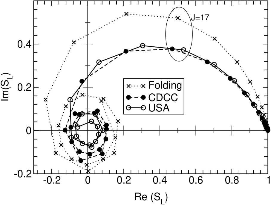
Figure 1: Argand plot for the CDCC (filled circles), USA (open circles) and cluster-folded (crosses) calculations, corresponding to the d+⁵⁸Ni elastic scattering at $E_{d}$=80 MeV.

The differential elastic angular distributions derived from the above $S$-matrices are shown in Fig. 2, along with the data of Stephenson et al. [13]. The dotted line represents the folding calculation, which clearly overestimates the data, particularly at intermediate angles. Inclusion of the continuum within the CDCC scheme (dashed line), produces a significant reduction of the elastic cross section and improves significantly the agreement with the data. Notice that, despite this improvement, the data are still somewhat overestimated at angles around 60^∘. Two different USA calculations are presented in Fig. 2. The first one, represented in the graph by the dotted–dashed line, was performed with a maximum hyperangular momentum $K_{m}$=30. This calculation agrees fairly well with the data in the whole angular range. Note that for $\theta_{\mathrm{c.m.}}<25^{\circ}$ the agreement with the data is excellent. At intermediate angles, the USA reproduces well the interference pattern, although the absolute normalization is somewhat underestimated. This suggests that the method will overestimate the breakup cross sections, as it will be discussed below. For c.m. angles above 80^∘ the USA calculation shows some oscillations, which are not present on neither the CDCC calculation nor the experimental data. These spurious wiggles are partially suppressed when the cutoff hyperangular momentum is increased to $K_{m}$=40, as shown by the solid line. We found that for higher values of $K_{m}$ the angular distribution remains basically unchanged. Thus, we can conclude that for $K_{m}$=40 we have convergence of the USA calculation.

Figure 2: Elastic scattering angular distribution for the d+⁵⁸Ni reaction at $E_{d}$=80 MeV. The meaning of the curves are indicated by the labels.

3.2 Breakup reaction

We next analyse the breakup channel for the same reaction. Due to the absence of experimental data, we will compare our model directly with CDCC.

We first study the integrated breakup cross section, as a function of the total angular momentum $J$. In the USA calculation, we can make use of the closed expression (33). The results are shown in Fig. 3. It can be seen that the USA calculation (solid line) reproduces the qualitative behaviour of the CDCC (dashed-line). In particular, both distributions predict a maximum of the breakup cross section at $J=17$. However, our model yields significantly more breakup than the CDCC, as we anticipated from the behaviour of the elastic angular distribution.

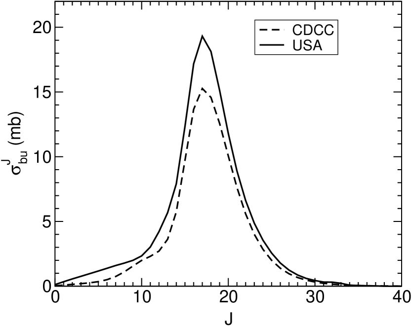
Figure 3: Integrated breakup cross section, as a function of the total angular momentum, $J$ for the reaction d+⁵⁸Ni at 80 MeV. The dashed and solid line correspond to the CDCC and USA calculations, respectively.

As described in the previous section, the method here developed provides also compact expressions for the partial integrated cross sections leading to continuum states with definite values of {$L^{\prime}$,$I^{\prime}$,$J$}, according to Eq. (32). Using the same physical ingredients as in the elastic scattering, we have applied this formula to calculate the integrated breakup cross section for $I^{\prime}$=0–12. The results are displayed by open circles in Fig. 4. It becomes clear that the main contribution to the breakup cross sections comes from the partial waves $I^{\prime}$=0 and $I^{\prime}$=2. Also included in this figure are the CDCC results (filled circles). Note that within CDCC these integrated cross sections are obtained as a result of large set of coupled equations, in which all possible values of $L^{\prime}$ and $I^{\prime}$ need to be coupled simultaneously. From this figure it becomes apparent that the discrepancy of the breakup cross section between the two methods is mainly due to the components $I^{\prime}$=0 and $I^{\prime}$=2. For $I^{\prime}>2$ the two methods are in excellent agreement. This result becomes more notable if one compares the simplicity of Eq. (32) with the large set of coupled-channels equations involved in the CDCC. Furthermore, when high excitation energies and angular momenta are to be included, convergence problems typically arise in CDCC. This is in contrast with Eq. (32), which allows one to calculate the breakup to highly excited states and large values of $I^{\prime}$ in a simple way without the numerical difficulties involved in a CDCC calculation.

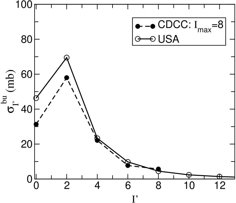
Figure 4: Integrated breakup cross section, as a function of the final p-n angular momentum, $I^{\prime}$. The filled circles (joined with dashed lines to guide the eye) correspond to the converged CDCC calculation ($I_{\max}=8$), while the open circles joined by solid lines are the USA prediction obtained with the closed expression (32).

Besides the integrated breakup cross sections, we can also calculate the breakup to specific states of the continuum. The $S$-matrix element describing the transition from the ground state to a continuum state with asymptotic linear momentum $p$ and angular momenta {$L^{\prime},I^{\prime},J$} is given by Eq. (30). Two different models where used to describe the continuum states within the USA method. In the first one, we used a discretized continuum in terms of continuum bins, as in the CDCC calculation. Since these bins are normalizable the overlaps $\langle\phi_{f}|K\rangle_{LI}$ appearing in Eq. (30) are calculated in exactly the same way as for the ground state. In a second calculation we used for the final states the true scattering wavefunctions, calculated at a given excitation energy. Note that these states are no longer normalizable and so special care has to be taken in order to calculate their overlaps with the hyperspherical basis. Details of the evaluation of these overlaps can be found in Appendix A. In this calculation, we found convenient, although not essential, to work with analytic expressions for the wavefunctions. In particular, for the ground state we used the Hulthèn wavefunction:

$$\phi_{0}(r)=\sqrt{\frac{\alpha\beta(\alpha+\beta)}{2\pi(\beta-\alpha)^{2}}}\frac{e^{-\alpha r}-e^{-\beta r}}{r},$$ (34)

with $\alpha=0.2317\,\mathrm{fm}^{-1}$ and $\beta=7\alpha$. For the continuum states, we used the solution of a separable potential, whose ground state coincides with the Hulthèn wave function, thus guaranteeing the orthogonality with the ground state wavefunction. These are explicitly given by

$$\phi^{(-)}_{\mathbf{p}}(\mathbf{r})=\frac{1}{(2\pi)^{3}}\left\{e^{i\mathbf{pr}}+f(p)\frac{e^{-ipr}-e^{-\beta r}}{r}\right\}\,,$$ (35)

with

$$f(p)=-\left[\beta-\frac{\beta^{2}+p^{2}}{2\beta}-\frac{(\beta^{2}+p^{2})^{2}}{2\beta(\alpha+\beta)^{2}}+ip\right]^{-1},$$ (36)

where $\alpha$ and $\beta$ are the same as for the ground state. These wavefunctions are normalized as $\langle\phi_{\mathbf{p}^{\prime}}|\phi_{\mathbf{p}}\rangle=\delta(\mathbf{p}^{\prime}-\mathbf{p})$. Note also that this potential acts only on the $s$-waves; for $I\neq 0$, the continuum sates are simply given by planes waves.

In Fig. 5, we compare the modulus of the breakup $S$-matrix for a total angular momentum $J=17$ which, according to Fig. 3, corresponds to the maximum of the breakup distribution. The continuum states with $I^{\prime}=0$ and $I^{\prime}=2$ have been considered for the comparison. In the latter, the separated contributions for $L^{\prime}$=15, 17 and 19 are shown. Two different CDCC calculations are presented. The first one, represented by open circles, uses a model space with $I=0,2$ only. However, this model space is not enough to achieve convergence of the $S$-matrix elements. In analogy with [10], we had to include partial waves up to $I_{\max}$=8. The results of this CDCC calculation in the augmented space is shown by the filled circles in Fig. 5. The USA calculations with the Hulthèn potential are represented in Fig. 5 by the solid lines. Finally, the USA calculation performed with the continuum bins is represented with a histogram, to emphasize the fact that this calculation uses a discretized continuum. Both calculations used a maximum hyperangular momentum $K_{m}$=30. With $K_{m}$=40 the results are only slightly changed. In general, we find a good global agreement between USA and CDCC. For small values of $p$ (i.e. low excitation energies) the two methods yield very similar results. On the contrary, for large values of $p$ all our calculations tend to predict more breakup than the CDCC. Interestingly, the USA distributions exhibit a bump at $p\approx$1 fm^-1 (i.e. $\epsilon\approx 41$ MeV), which is not observed in the converged CDCC with $I_{\max}$=8, but appears nevertheless in the CDCC with $I_{\max}$=2. The major disagreement between the USA and CDCC occurs for the breakup to $s$ states. In this case, the two methods give very different predictions for $p>0.3$ fm^-1.

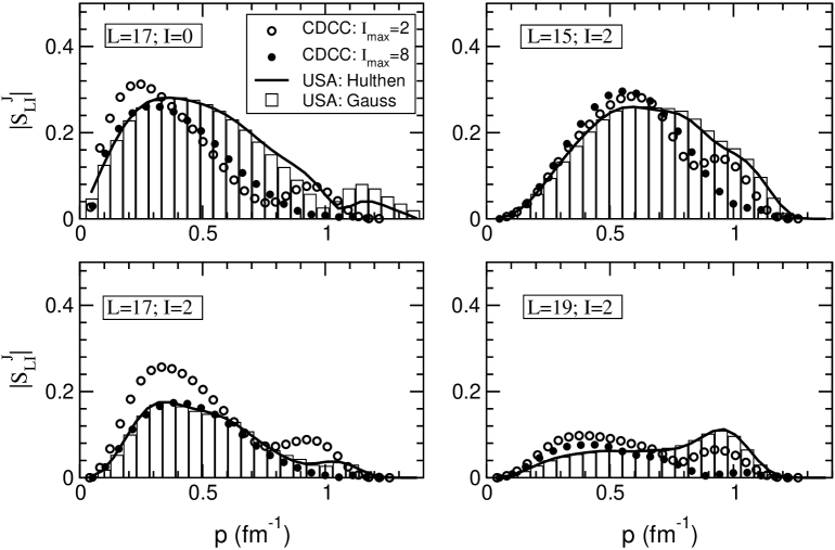
Figure 5: Breakup $S$-matrix elements for a total angular momentum $J=17$ and final p-n relative angular momentum $I^{\prime}$=0 and 2. The filled circles correspond to the CDCC calculation with $s$ and $d$ waves only, whereas the open circles are the CDCC calculations with the model space $I=0,2,4,6,8$. The solid line is the USA calculation with analytic wavefunctions derived from a separable potential. The histogram correspond to the USA calculation using the bins constructed with Gaussian potential.

The differential breakup cross section is readily calculated from the above $S$-matrix elements using Eq. (31), and summing upon $L^{\prime}$ and $J$. The results are displayed in Fig. 6. The filled circles correspond to the CDCC calculation in the model space with $I_{\max}$=8. The solid line is the USA calculation with the p-n separable interaction. The histogram corresponds to the USA calculation in the discretized continuum, generated with the Gaussian potential. We see that, at small excitation energies, the USA and CDCC calculations are in very good agreement. At higher excitation energies, the USA predicts systematically more breakup, as expected from the behaviour of the $S$-matrices analysed above. For $I^{\prime}=6$, the USA calculations obtained with the continuum bins agree nicely with the CDCC. In the cases $I^{\prime}$=0 and $I^{\prime}$=2 we show also the adiabatic coupled–channels calculation by Amakawa and Tamura [16]. This calculation follows a similar trend to that of the CDCC, which is understood by recalling that the adiabatic approximation can be regarded to an approximated CDCC calculation in which the internal Hamiltonian is replaced by a constant [9].

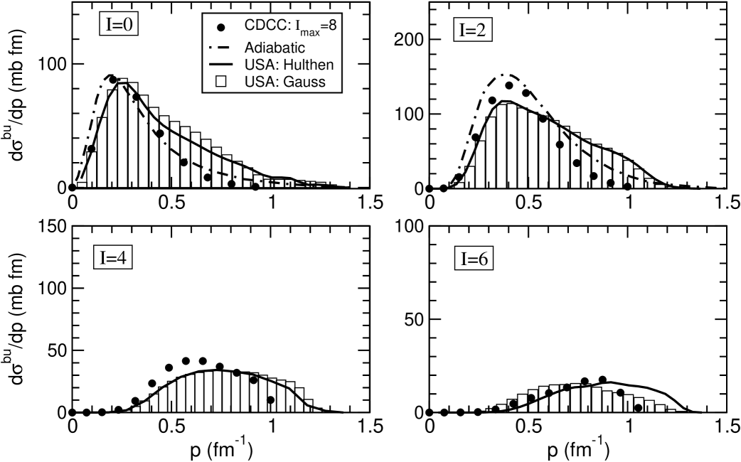
Figure 6: Breakup excitation function for the reaction d+⁵⁸Ni at $E_{d}$=80 MeV. The filled circles represent the CDCC calculations. The solid lines are the USA calculations with the Hulthèn wavefunctions. The histogram is the USA calculation obtained with a Gaussian potential and a discretized continuum. The dotted-dashed lines are the adiabatic calculation of Amakawa and Tamura [16].

From the analysis performed in this section, we conclude that, despite its formal simplicity, the model developed in this work provides a good description of the reaction observables. In particular, we have shown that the method describes fairly well the elastic and breakup scattering of d+$\@@nuc{58}{Ni}$ at $E_{d}$=80 MeV. Our comparison with the CDCC calculations suggests that the USA tends to overestimate breakup to highly excited states on the continuum.

In comparing the CDCC calculation with the USA results, it should be taken into account that the USA approach is not simply an approximation to the CDCC calculation. The latter is performed assuming that the interactions between fragments and target, that are complex, can be approximated by local potentials. This determines the off-shell behaviour of the interaction and, in particular, prevents coupling to highly excited states of the projectile. In contrast, the USA approximation relies on the fact that off-shell matrix elements of the interaction are substituted by on-shell ones. This seems to be the reason behind the larger breakup cross sections to highly excited states.

4 Summary and conclusions

In this paper we have revisited the uncorrelated scattering approximation (USA) originally introduced in Ref. [6]. We reviewed the basic assumptions involved within the USA approach and analyzed its capability to describe elastic and breakup scattering reactions. In what follows we summarize the main ingredients and results obtained in this work.

The description of the scattering reaction mechanism provided by the USA model is based on three basic approximations. First, in the case of a weakly bound system interacting with a heavy target, we ignore the interaction between the fragments in the three-body $T$-matrix propagator. Thus, the operator $T(E)$ may be replaced by $\bar{T}(E)/\lambda$, being $\bar{T}(E)$ the uncorrelated $T$-matrix for a renormalized interaction. This has the property to conserve the angular momentum of each fragment of the projectile with respect to the target. However, it results essential to conserve the interaction in the asymptotic states, which are eigenstates of the Hamiltonian $H_{0}$. Expanding these states into eigenstates of $\bar{H}_{0}$ (Hamiltonian containing only kinetic energy terms), one finally ends up with the evaluation of the off–shell $\bar{T}(E)$ matrix elements.

The second approximation involved is to replace the off–shell matrix elements of $\bar{T}(E)$ by the on-shell ones. This is justified because the range of off-shellness in the matrix element is small compared with the energy range of the operator. However, a direct substitution of the off shell matrix element by on-shell ones may lead to the breakdown of the unitarity property. Thus, in this work we have made use of a renormalization operator, which is formally equivalent to the Democratic Mapping procedure described in [17]. The matrix elements of $\bar{T}(E)$ between eigenstates of $\bar{H}_{0}$ can be evaluated using an expansion in hyperspherical harmonics. This allows us to transform analytically the asymptotic states into states with definite values of the angular momenta $L_{A}$ and $L_{B}$ of each fragment with respect to the target, and take advantage of the fact that these magnitudes are conserved by the interaction.

The third approximation is to expand up to third order the three-body operator $\bar{T}(E)$ in terms of the three-body operators $T_{A}(E)$ and $T_{B}(E)$ which contain only the interaction of one of the particles with the target. Then the on-shell matrix elements of $\bar{T}(E)$ can be evaluated, and the result shows that the operator $\bar{T}(E)$ does not connect states in which the total energy $E$ is distributed differently between particles $A$ and $B$. Moreover, the matrix element of $\bar{T}(E)$ is completely determined by the on-shell matrix elements of the two-body operators ${\mathbf{t}}_{A}(e_{A})$ and ${\mathbf{t}}_{B}(e_{B})$ evaluated at the corresponding energies of the two particles.

Our analysis shows that the $S$-matrix describing the scattering of a composite system by a target, in the uncorrelated scattering approximation, is given as a combination of products of the $S$-matrices describing the scattering of the fragments evaluated at the corresponding energies and angular momenta. The renormalization factor $\lambda$ can be obtained for each $J$ value to ensure that, in the weak coupling limit, the USA reproduces the elastic scattering calculated with the folding interaction. This renormalization factor allows us to include the effect of excitation of the target and/or the fragments of the projectile, which is essential in nuclear collisions, in a way which is fully consistent with a complex folding interaction.

The USA keeps also some resemblance with other impulse approximations recently applied to the scattering of weakly bound nuclei [18, 19]. In analogy with the multiple scattering of the $T$-matrix method presented in [19], we start with an approximated expansion of the few–body $T$-matrix, in which the inter-cluster interaction is neglected in the propagator. However, while in [19] the derivation is performed in a linear momentum representation, we choose a partial wave description. Moreover, although both methods express the total $T$-matrix in terms of two-body amplitudes, the approximations that lead to the two–body $T$-matrices are quite different.

There exists also some formal analogy between our main result, Eq. (LABEL:norts), and the semiclassical Glauber approximation [3], in the sense that in both methods the scattering amplitude depends on a superposition of the product of the individual $S$-matrices of the fragments. However, despite this apparent similitude, we stress that the approximations involved in both approaches are very different. First, unlike the Glauber model, the USA does not make any semiclassical assumption. Furthermore, the Glauber model is based on the frozen halo or adiabatic approximation (i.e., it neglects the excitation energies of the internal Hamiltonian), while the USA neglects the inter-cluster potential (the so called impulse approximation), but retains the full kinetic energy operator.

Finally, it should be stressed that the main differences found between the USA and the CDCC calculations arise from the fact that the USA calculation gives rise to larger breakup cross sections to states with high excitation energies. This result might be related to limitations of the USA approach, but it could also be due to the fact that the CDCC calculations assume local interactions between the fragments of the projectile and the target, and this determines the off-shell nature of the interactions. Accurate experimental measurements of breakup cross sections at high excitation energies would surely help to draw more definite conclusions on the validity of the local, momentum independent, complex interactions used in the CDCC approach or, by contrast, on the reliability of the presence of relevant off-shell components in the interaction as suggested by the USA calculations.

Appendix A Expansion of the channel wavefunctions in terms of the hyperangle

The bound states of the projectile, as well as the normalizable bins of continuum states, can be expressed in momentum representation as

$$|\phi_{i};IM_{I}\rangle=\int dq\phi_{i}(q)|q;IM_{I}\rangle\,,$$ (37)

where the state $|q;IM_{I}\rangle$ is normalized so that $\langle q^{\prime};IM_{I}|q;IM_{I}\rangle=\delta(q-q^{\prime})$. The corresponding channel states can be written as

$$|\phi_{i},k_{i};I,L,J\rangle=\int dq\phi_{i}(q)|q,k_{i};I,L,J\rangle\,.$$ (38)

It is convenient to write this state in terms of states with given hyperangle $\alpha$ and kinetic energy $E_{i}(\alpha)$, which are given by

$$\tan(\alpha)={q\over k_{i}}\sqrt{M\over\mu},\quad E_{i}(\alpha)={\hbar^{2}q^{2}\over 2\mu}+{\hbar^{2}k_{i}^{2}\over 2M}\,,$$ (39)

which leads to

$$|\phi_{i},k_{i};L;I,J\rangle = \int d\alpha g_{i}(\alpha)|\alpha,E(i,\alpha);L;I,J\rangle$$ (40)

$$g_{i}(\alpha) = \phi_{i}(q(k_{i},\alpha))\left({dq(k_{i},\alpha)\over d\alpha}\right)^{1/2}\,.$$ (41)

The last term arises from the normalization $\langle\alpha^{\prime},E|\alpha,E\rangle=\delta(\alpha^{\prime}-\alpha)$.

The continuum states with asymptotic momentum $p$ are given by

$$|\phi(p),k(p);I,L,J\rangle=|p,k(p);I,L,J\rangle+\int dqg^{(}-)(p,q)|q,k(p);I,L,J\rangle\,,$$ (42)

where the first term in the RHS represents the plane wave and the second term represents incoming waves. The integral has a pole at $q=p$, with a residue $R(p)$ and a principal part, so

$$|\phi(p),k(p);I,L,J\rangle = [1+i\pi R(p)]|p,k(p);I,L,J\rangle$$ (43)

$$+ {\mathcal{P}}\int dqg^{(}-)(p,q)|q,k(p);I,L,J\rangle\,.$$

This state can be written in terms of the hyperangle as

$$|\phi(p),k(p);I,L,J\rangle = [1+i\pi R(p)]\left({dp\over d\alpha_{p}}\right)^{1/2}|\alpha_{p},E;I,L,J\rangle$$

$$+ {\mathcal{P}}\int d\alpha g^{(}-)(p,q(\alpha))\left({dq\over d\alpha}\right)^{1/2}|\alpha,E(p,\alpha);I,L,J\rangle\,,$$

where

$$\tan(\alpha_{p})={p\over k(p)}\sqrt{M\over\mu}, E={\hbar^{2}p^{2}\over 2\mu}+{\hbar^{2}k(p)^{2}\over 2M}\,,$$ (45)

$$\tan(\alpha)={q\over k(p)}\sqrt{M\over\mu}, \quad E(p,\alpha)={\hbar^{2}q^{2}\over 2\mu}+{\hbar^{2}k(p)^{2}\over 2M}\,.$$ (46)

Appendix B On-shell matrix elements in the hyperspherical basis

In this appendix we show in detail the procedure used to evaluate the on-shell matrix elements of the operator $\bar{T}(E)$. First, we make use of an expansion in hyperspherical harmonics which allows us to write down

$$\int d\alpha g^{I}_{i}(\alpha)A^{i}(\alpha)|\alpha,E;L,I,J\rangle=\sum_{K}\langle K|\phi_{i}\rangle_{LI}|K,E;L,I,J\rangle\,,$$ (47)

where we introduce the states

$$|K,E;L,I,J\rangle=\int_{0}^{\pi/2}d\alpha f^{K}_{L,I}(\alpha)|\alpha,E;L,I,J\rangle.$$ (48)

The functions $f^{K}_{L,I}(\alpha)$ are given by

$$f_{L,I}^{K}(\alpha)=N^{LI}_{K}(\cos\alpha)^{L+1}(\sin\alpha)^{I+1}P^{(I+\frac{1}{2},L+\frac{1}{2})}_{(K-L-I)/2}(\cos 2\alpha),$$ (49)

where $P^{(I+\frac{1}{2},L+\frac{1}{2})}_{n}$ are the Jacobi polynomials of degree $n$ and $N^{LI}_{K}$ are some normalization constants, whose explicit expressions can be found in [6].

The coefficients $\langle K|\phi_{i}\rangle_{LI}$ are explicitly given by

$$\langle K|\phi_{i}\rangle_{LI} = \sum_{K^{\prime}}c^{i}_{LI}(K^{\prime})A^{i}_{LI}(K^{\prime},K)$$ (50)

$$c^{i}_{LI}(K^{\prime}) = \int d\alpha f^{K^{\prime}}_{L,I}(\alpha)g^{I}_{i}(\alpha)$$ (51)

$$A^{i}_{LI}(K^{\prime},K) = \int d\alpha f^{K^{\prime}}_{L,I}(\alpha)A^{i}(\alpha)f^{K}_{L,I}(\alpha)\,.$$ (52)

To get these expressions we have made use of the closure property of the hyperspherical harmonics

$$\sum_{K}f^{K}_{L,I}(\alpha)f^{K}_{L,I}(\alpha^{\prime})=\delta(\alpha-\alpha^{\prime})\,.$$ (53)

Then, we end up with the following expression for the $T$-matrix elements

$$\langle\phi_{f},k_{f};L^{\prime},I^{\prime},J|T(E)|\phi_{g},k_{g};L,I,J\rangle\simeq$$

$$\sum_{K^{\prime},K}\langle\phi_{f}|K^{\prime}\rangle_{L^{\prime}I^{\prime}}\langle K|\phi_{g}\rangle_{LI}\langle K^{\prime},E;L^{\prime},I^{\prime},J|\bar{T}(E)|K,E;L,I,J\rangle\,.$$ (54)

The requirement that the approximated expression preserves unitarity for hermitian interactions leads to

$$\sum_{i}\langle K^{\prime}|\phi_{i}\rangle_{LI}\langle\phi_{i}|K\rangle_{LI}=\delta_{K,K^{\prime}}\,.$$ (55)

On the other hand, if the interaction is constant, the matrix elements of $\bar{T}(E)$ will be diagonal and independent on $K$. In this case, the $T$-matrix should not couple different internal states. This leads to

$$\sum_{K}\langle K|\phi_{g}\rangle_{LI}\langle\phi_{f}|K\rangle_{LI}=\delta_{g,f}\,.$$ (56)

These conditions can be achieved by an adequate choice of $A^{i}_{LI}(K^{\prime},K)$. In what follows we shall assume, for definiteness, that in each spin channel $I$ there is at most one bound state, while the rest of the states correspond to the continuum. So, for the bound state in channel $I$ we take

$$A^{b}_{LI}(K,K^{\prime}) = \delta_{K,K^{\prime}}/\sqrt{P^{b}_{LI}}\,,$$ (57)

with $P^{b}_{LI}=\sum_{K}|c^{b}_{LI}(K)|^{2}$, while for the rest of the states in channel $I$ we consider a unique symmetric matrix $A^{c}_{LI}(K^{\prime},K)$ which fulfils

$$\sum_{K^{\prime}}A^{c}_{LI}(K,K^{\prime})c^{b}_{LI}(K^{\prime})=0\,,$$ (58)

$$\sum_{K_{1},K^{\prime}_{1}}A^{c}_{LI}(K,K_{1})A^{c}_{L,I}(K^{\prime},K^{\prime}_{1})\sum_{i\neq b}c^{i*}_{LI}(K_{1})c^{i}_{LI}(K^{\prime}_{1})=\delta_{K,K^{\prime}}-\frac{c^{b}_{LI}(K)c^{b}_{LI}(K^{\prime})}{P^{b}_{LI}}\,.$$

Note that this procedure is equivalent to orthogonalize all the continuum states with respect to the ground state, and then apply the “democratic mapping” procedure to the continuum states.

It should be noticed that the sum in $K$ is extended in principle up to infinity. Note that in this case $P^{b}_{L,I}=1$. In practice, the sum is taken up to a maximum value $K_{m}$, which is obtained to get convergence in the calculations. So, in general, $P^{b}_{L,I}\leq 1$, specially for the higher partial waves, for which $L$ is close to $K_{m}$. Note that, in contrast to what was done in Ref. [6, 20], no physical meaning is attached to the parameter $K_{m}$, which should be taken as large as possible, until convergence is achieved.

In order to make use of the fact that $\bar{T}(E)$ conserves the angular momenta of the fragments, one can use the Raynal-Revai transformation [7]:

$$|K,E;L,I,J\rangle=\sum_{L_{A},L_{B}}|K,E;L_{A},L_{B},J\rangle\langle L_{A},L_{B}|L,I\rangle_{KJ}\,.$$ (60)

The states with different $K$ values can be expanded to get states with definite values of the kinetic energy of each fragment. We can write, in terms of the hyperangle,

$$|K,E;L_{A},L_{B},J\rangle=\int d\beta f^{K}_{L_{A},L_{B}}(\beta)|\beta,E;L_{A},L_{B},J\rangle\,.$$ (61)

This state can be characterized in terms of a product state of particles $A$ and $B$ with energies $e_{A}=E\cos^{2}(\beta)$ and $e_{B}=E\sin^{2}(\beta)$.

Appendix C Multiple scattering expansion of the $\bar{T}$ operator

In this appendix we evaluate the on-shell matrix elements $\langle\beta^{\prime},E|\bar{T}(E)|\beta,E\rangle$, where the state $|\beta,E\rangle$ is an eigenstate of $\bar{H}_{0}=K_{A}+K_{B}$, corresponding to energies $e_{A}=E\cos^{2}\beta$ and $e_{B}=E\sin^{2}\beta$. Analogously, the state $|\beta^{\prime},E\rangle$ corresponds to $e^{\prime}_{A}=E\cos^{2}\beta^{\prime}$ and $e^{\prime}_{B}=E\sin^{2}\beta^{\prime}$. Note that $E=e_{A}+e_{B}=e^{\prime}_{A}+e^{\prime}_{B}$. We can write explicitly

$$|\beta,E\rangle=N(\beta)|e_{A},e_{B}\rangle\,,$$ (62)

where $N(\beta)=\sqrt{E\sin(2\beta)}$ is the square root of the Jacobian of the transformation from $\{e_{A},e_{B}\}$ to $\{\beta,E\}$.

We consider the multiple scattering expansion of the operator $\bar{T}(E)$ up to third order

$$\bar{T}(E) = T_{A}(E)+T_{B}(E)$$

$$+ T_{A}(E)\bar{G}_{0}(E)T_{B}(E)+T_{B}(E)\bar{G}_{0}(E)T_{A}(E)$$

$$+ T_{A}(E)\bar{G}_{0}(E)T_{B}(E)\bar{G}_{0}(E)T_{A}(E)+T_{B}(E)\bar{G}_{0}(E)T_{A}(E)\bar{G}_{0}(E)T_{B}(E)\,,$$

where $\bar{G}_{0}(E)=(E^{+}-K_{A}-K_{B})^{-1}$ is the free 3-body propagator and

$$T_{A}(E)=\lambda v_{AT}+\lambda v_{AT}\bar{G}_{0}(E)T_{A}(E)\,.$$ (64)

The matrix operator $T_{A}(E)$ can change the kinetic energy of particle $A$, through its off–shell components, but it can not modify the kinetic energy of $B$. Hence, we can write

$$\langle\beta^{\prime},E|T_{A}(E)|\beta,E\rangle=\delta(\beta-\beta^{\prime})\langle e_{A}|{\bf t}_{A}(e_{A})|e_{A}\rangle\,,\\$$ (65)

where we have introduced the operator

$${\bf t}_{A}(e_{A})=\lambda v_{AT}+\lambda v_{AT}g_{A}(e_{A}){\bf t}_{A}(E),$$ (66)

with $g_{A}(e)=(e^{+}-K_{A})$ the free 2-body propagator. Note that the operators $T_{A}$ and ${\bf t}_{A}$ differ on the kinetic operator appearing in the propagator. While $T_{A}$ is defined with the full kinetic energy operator, i.e., $K_{A}+K_{B}$, the propagator in ${\bf t}_{A}$ contains only the kinetic energy operator associated with particle $A$, $K_{A}$. Therefore, $T_{A}$ should be understood as a three-body operator, whereas ${\bf t}_{A}$ corresponds to a two-body operator. For simplicity, in the following, we drop the energy argument of the three-body operators $T_{A},T_{B},\bar{G}_{0}$, which is in all cases $E$, but we retain it in the two-body operators.

The contribution of the second order terms can be expressed as the sum of a pole term and a principal part

$$\langle\beta^{\prime},E|T_{A}\bar{G}_{0}T_{B}|\beta,E\rangle = i\pi\delta(\beta-\beta^{\prime})t_{A}(e_{A})t_{B}(e_{B})$$ (67)

$$+ {\langle e_{A}^{\prime}|{\bf t}_{A}(e^{\prime}_{A})|e_{A}\rangle\langle e^{\prime}_{B}|{\bf t}_{B}(e_{B})|e_{B}\rangle\over E-e^{\prime}_{B}-e_{A}}N(\beta)N(\beta^{\prime})\,,$$

$$\langle\beta^{\prime},E|T_{B}\bar{G}_{0}T_{A}|\beta,E\rangle = i\pi\delta(\beta-\beta^{\prime})t_{A}(e_{A})t_{B}(e_{B})$$ (68)

$$+ {\langle e^{\prime}_{B}|{\bf t}_{B}(e^{\prime}_{B})|e_{B}\rangle\langle e^{\prime}_{A}|{\bf t}_{A}(e_{A})|e_{A}\rangle\over E-e^{\prime}_{A}-e_{B}}N(\beta)N(\beta^{\prime})\,,\$$

where we have introduced the short notation $t_{A}(e_{A})$ and $t_{B}(e_{B})$ for the on-shell matrix elements $\langle e_{A}|{\bf t}_{A}(e_{A})|e_{A}\rangle$ and $\langle e_{B}|{\bf t}_{B}(e_{B})|e_{B}\rangle$, respectively.

As for the third order terms we have

$$\langle\beta^{\prime},E|T_{A}\bar{G}_{0}T_{B}\bar{G}_{0}T_{A}|\beta,E\rangle$$ (69)

$$= \int de^{\prime\prime}_{A}\langle e^{\prime}_{A}|t_{A}(e^{\prime}_{A})|e^{\prime\prime}_{A}\rangle\frac{1}{E^{+}-e^{\prime\prime}_{A}-e^{\prime}_{B}}\langle e^{\prime}_{B}|t_{B}(E-e^{\prime\prime}_{A})|e_{B}\rangle$$

$$\times \frac{1}{E^{+}-e^{\prime\prime}_{A}-e_{B}}\langle e^{\prime\prime}_{A}|t_{A}(e_{A})|e_{A}\rangle N(\beta)N(\beta^{\prime})\,.$$

To evaluate this contribution we make use of the following identities

$$g_{A}(e^{\prime})g_{A}(e) = \frac{1}{e-e^{\prime}}\Big{(}g_{A}(e^{\prime})-g_{A}(e)\Big{)}$$ (70)

$$t_{A}(e^{\prime})-t_{A}(e) = t_{A}(e^{\prime})\Big{(}g_{A}(e^{\prime})-g_{A}(e)\Big{)}t_{A}(e)\,.$$ (71)

The second of these expressions indicates that the operator $t_{B}(E-e^{\prime\prime}_{A})$ can be approximated by $t_{B}(e_{B})$, and the difference would be of higher order in the $T$-matrix expansion. Thus, one may write

$$\langle\beta^{\prime},E|T_{A}\bar{G}_{0}T_{B}\bar{G}_{0}T_{A}|\beta,E\rangle$$

$$\simeq\langle e^{\prime}_{B}|{\bf t}_{B}(e_{B})|e_{B}\rangle\langle e^{\prime}_{A}|{\bf t}_{A}(e^{\prime}_{A})g_{A}(e^{\prime}_{A})g_{A}(e_{A}){\bf t}_{A}(e_{A})|e_{A}\rangle N(\beta)N(\beta^{\prime})\,.$$ (72)

Making use of the above identities, one gets

$$\langle\beta^{\prime},E|T_{A}\bar{G}_{0}T_{B}\bar{G}_{0}T_{A}|\beta,E\rangle$$ (73)

$$\simeq \langle e^{\prime}_{B}|{\bf t}_{B}(e_{B})|e_{B}\rangle\frac{\langle e^{\prime}_{A}|{\bf t}_{A}(e^{\prime}_{A})|e_{A}\rangle-\langle e^{\prime}_{A}|{\bf t}_{A}(e_{A})|e_{A}\rangle}{e_{A}-e^{\prime}_{A}}N(\beta)N(\beta^{\prime})\,.$$

A similar derivation for the other third order term gives

$$\langle\beta^{\prime},E|T_{B}\bar{G}_{0}T_{A}\bar{G}_{0}T_{B}|\beta,E\rangle$$ (74)

$$\simeq \langle e^{\prime}_{A}|{\bf t}_{A}(e_{A})|e_{A}\rangle\frac{\langle e^{\prime}_{B}|{\bf t}_{B}(e^{\prime}_{B})|e_{B}\rangle-\langle e^{\prime}_{B}|{\bf t}_{B}(e_{B})|e_{B}\rangle}{e_{B}-e^{\prime}_{B}}N(\beta)N(\beta^{\prime})\,.$$

So, the sum of the two third order contributions reduces to

$$\langle\beta^{\prime},E|T_{A}\bar{G}_{0}T_{B}\bar{G}_{0}T_{A}|\beta,E\rangle+\langle\beta^{\prime},E|T_{B}\bar{G}_{0}T_{A}\bar{G}_{0}T_{B}|\beta,E\rangle$$

$$=\frac{\langle e^{\prime}_{B}|{\bf t}_{B}(e_{B})|e_{B}\rangle\langle e^{\prime}_{A}|{\bf t}_{A}(e^{\prime}_{A})|e_{A}\rangle}{e_{A}-e^{\prime}_{A}}N(\beta)N(\beta^{\prime})$$

$$+\frac{\langle e^{\prime}_{A}|{\bf t}_{A}(e_{A})|e_{A}\rangle\langle e^{\prime}_{B}|{\bf t}_{B}(e^{\prime}_{B})|e_{B}\rangle}{e_{B}-e^{\prime}_{B}}N(\beta)N(\beta^{\prime})\,,$$ (75)

which cancels exactly the principal value part of the second order terms, Eqs. (67) and (68). Therefore, collecting these results, we have that the on-shell matrix elements of the $\bar{T}$ operator up to third order can be written as

$$\langle\beta^{\prime},E|\bar{T}(E)|\beta,E\rangle=\delta(\beta-\beta^{\prime})\Big{\{}t_{A}(e_{A})+t_{B}(e_{B})+2i\pi t_{A}(e_{A})t_{B}(e_{B})\Big{\}}\,.$$

References

- [1] P. G. Hansen, A. Jensen, B. Jonson, Ann. Rev. Nucl. Part. Sci. 45 (1995) 591.
- [2] M. Zhukov et al., Phys. Rep. 231 (1993) 151.
- [3] R. Glauber, in: Lectures in Theoretical Physics, Edited by W.E. Brittin, Interscience, New York, 1959, p. 315.
- [4] R. C. Johnson, Proceedings of the European Conference on Advances in Nuclear Physics and Related Areas, Thessaloniki, Greece, 1997 (unpublished).
- [5] R. C. Johnson, J. S. Al-Khalili, J. A. Tostevin, Phys. Rev. Lett. 79 (1997) 2771.
- [6] A. M. Moro, J. A. Caballero, J. Gómez-Camacho, Nucl. Phys. A 695 (2001) 143.
- [7] J. Raynal, J. Revai, Nuovo Cim. 68A (1970) 612.
- [8] A. M. Moro, Ph.D. Thesis, University of Sevilla. Unpublished.
- [9] N. Austern, Y. Iseri, M. Kamimura, M. Kawai, G. Rawitscher, M. Yahiro, Phys. Rep. 154 (1987) 125.
- [10] R. Piyadasa, M. Kawai, M. Kamimura, M. Yahiro, Phys. Rev. C 60 (1999) 044611.
- [11] Y. Iseri, M. Yahiro, M. Kamimura, Prog. Theor. Phys. Suppl. 89 (1986) 84.
- [12] M. Yahiro, Y. Iseri, H. Kameyama, M. Kamimura, M. Kawai, Prog. Theor. Phys. Suppl. 89 (1986) 32.
- [13] E. J. Stephenson et al., Phys. Rev. C 28 (1983) 134.
- [14] F. Becchetti, G. Greenlees, Phys. Rev. 182 (1969) 1190.
- [15] I. J. Thompson, Comp. Phys. Rep. 7 (1988) 167.
- [16] H. Amakawa, T. Tamura, Phys. Rev. C 26 (1982) 904.
- [17] L. D. Skouras et al., Nucl. Phys. A 516 (1990) 255.
- [18] R. Crespo, R. C. Johnson, Phys. Rev. C 60 (1999) 034007.
- [19] R. Crespo, I. J. Thompson, Phys. Rev. C 63 (2001) 044003.
- [20] A. M. Moro, J. A. Caballero, J. Gómez-Camacho, Nucl. Phys. A689 (2001) 547c.