Covariant Effective Field Theory for Nuclear Structure
and Nuclear Currents

1 Introduction

The fundamental theory of the strong interaction is quantum chromodynamics (QCD), which is a relativistic field theory with local gauge invariance, whose elementary constituents are colored quarks and gluons. In principle, QCD should provide a complete description of nuclear structure and dynamics. Unfortunately, QCD predictions at nuclear length scales with the precision of existing (and anticipated) experimental data are not available, and this state of affairs will probably persist for some time. Even if it becomes possible to use QCD to describe nuclei directly, this description is likely to be cumbersome and inefficient, since quarks cluster into hadrons at low energies.

How can we simplify this problem to make progress? We will employ a framework based on Lorentz-covariant, effective quantum field theory and density functional theory. Effective field theory (EFT) embodies basic principles that are common to many areas of physics, such as the natural separation of length scales in the description of physical phenomena. In EFT, the long-range dynamics is included explicitly, while the short-range dynamics is parametrized generically; all of the dynamics is constrained by the symmetries of the interaction. When based on a local, Lorentz-invariant Lagrangian (density), EFT is the most general way to parametrize observables consistent with the principles of quantum mechanics, special relativity, unitarity, gauge invariance, cluster decomposition, microscopic causality, and the required internal symmetries.

Density functional theory (DFT), which has been widely used in atomic and condensed-matter physics, allows us to describe the nuclear many-body system with a universal energy functional that depends on nuclear densities and four-vector currents. In principle, knowledge of the full energy functional allows us to calculate any observable for the (zero-temperature) many-body system; moreover, a simplified treatment of the functional based on quasi-particle orbitals still provides an exact description of bulk nuclear properties and some single-particle observables. The great advantage of DFT is that calculations of this subset of properties can be made without knowledge of the many-body wave function, or with a simple one. Finally, if relevant expansion parameters can be found, the energy functional can be truncated to a manageable size, and the accuracy of the truncation can be tested quantitatively for the observables in question.

The basic properties of nuclei provide stringent constraints on any nuclear theory. An accurate description of these properties is necessary for any useful predictions or extrapolations. We certainly want to reproduce the observed shapes of nuclei: the interior density of a heavy nucleus should be relatively constant, there should be a well-defined surface, and because of nuclear “saturation”, the radius $R$ of a nucleus should scale according to $R\propto B^{1/3}$, where $B=N+Z$ is the total number of neutrons and protons. Moreover, the total energy $E$ of the nucleus should agree with the “liquid drop” formula

$$E=-{a_{1}}B+{a_{2}}B^{2/3}+{a_{3}}Z^{2}/B^{1/3}+{a_{4}}(N-Z)^{2}/B+\cdots\ ,$$ (1)

where typical values for the $a_{i}$ coefficients are given in [1, 2, 3].

The particle spectrum is determined by the qualitative features of the single-particle potential. In nonrelativistic (Schrödinger) terminology, the central potential is midway between a harmonic oscillator and a square well; this shape determines the ordering of the levels as a function of the orbital angular momentum. (See [1], Figs. 57.1 and 57.2.) In addition, the spin-orbit potential is strong, which is instrumental in determining the major shell closures and, hence, the nuclear shell model. We will see later how these features are easily reproduced in a description based on the Dirac equation.

These simple nuclear features are the ones we will focus on. We expect that they can be adequately described by a single-particle equation with an effective, one-body interaction. Such an approach has many names, depending on the system being studied and on the practitioner: “shell model”, “mean-field theory”, “Kohn–Sham” DFT, etc. Our goal is to correlate (fit) a modest number of nuclear bulk and single-particle data and then to predict other, similar data as well as possible.

1.1 Why Use Hadrons?

Well, why not? Our focus is on low-energy, long-range nuclear characteristics, and all measured observables are colorless. (In fact, most of the observables of interest to us are dominated by the isoscalar part of the interaction.) Moreover, hadronic variables (baryons and mesons) are efficient, since hadrons are the particles that are observed in experiments. Colored quarks and gluons participate only in intermediate states, and such “off-shell behavior” is unobservable; by using hadrons, we expend no theoretical effort combining quarks and gluons into color singlets that can actually be observed.

So we pick the most efficient degrees of freedom by choosing hadrons. We will have to parametrize the nuclear EFT Lagrangian anyway, since we cannot compute its true form from QCD, and hadronic variables, if combined in all forms consistent with the underlying symmetries, provide sufficient flexibility for our parametrization. We cannot guarantee that a single-particle hadronic approach will be successful in describing all of the observables of interest, but we want to see how well we can do.

1.2 Why Use the Dirac Equation?

To motivate the Dirac equation as straightforwardly as possible, compare the particle spectrum (and fine structure) in a light atom with the spectrum in a heavy nucleus. An example of the former is given in [4], while an early example of the latter is given in [5], which is reproduced in Fig. 57.3 of [1]. The most striking result is that it is impossible to draw the atomic fine structure to scale, since the splittings are roughly 1/10,000 as large as the major-level splittings (at least for the deeply bound atomic levels). In contrast, the nuclear spectrum shows that the “fine” structure is really “gross”; the spin-orbit splittings are as large as the major-level splittings to within a factor of two!

The implication is that there must be some relativistic effects that are important in nuclei (unlike light atoms), and thus it is much more natural to use the Dirac equation to describe the quasi-particle nucleon wave functions.

1.3 Quantum Hadrodynamics (QHD)

We will refer to Lorentz-covariant, meson–baryon, effective field theories of the nuclear many-body problem as “quantum hadrodynamics” or QHD [3, 6, 7, 8, 9, 10, 11, 12, 13]. When QHD is applied within the framework of modern EFT and DFT, it provides a quantitative description of bulk nuclear properties and the spin-orbit force throughout the Periodic Table [9, 14, 11]. This success arises from the presence of large Lorentz scalar and vector mean fields, which imply that there are large relativistic interaction effects in nuclei under normal conditions [12]. There is evidence from QCD sum rules that these large fields are dynamical consequences of the underlying chromodynamics [15, 16]. Moreover, similar relativistic effects are responsible for the efficient description of spin observables in medium-energy proton–nucleus scattering using the Relativistic Impulse Approximation [17], and they are consistent with the major role played by scalar and vector meson exchange in modern boson-exchange models of the nucleon–nucleon (NN) interaction [18]. All of these features motivate further investigation into the application of QHD to the nuclear many-body problem.

2 Effective Field Theory

A modern discussion of QHD begins by interpreting the Lagrangian as defining a nonrenormalizable, effective field theory (EFT) [19, 9]. An effective Lagrangian consists of known long-range interactions constrained by symmetries and a complete, non-redundant set of generic short-range interactions (i.e., “contact” and “gradient” terms). The division between “long” and “short” is characterized by the breakdown scale $\Lambda$ of the EFT. While it is not possible at present to derive an effective hadronic theory directly from the underlying QCD, the EFT perspective implies that this is not necessary. If one constructs a general Lagrangian that respects the symmetries of QCD: Lorentz covariance, parity conservation, time-reversal and charge-conjugation invariance, (approximate) isospin symmetry, and spontaneously broken chiral symmetry, then the EFT is a general parametrization of observables below the breakdown scale.

For QHD, we identify $\Lambda$ with the mass scale of physics beyond the Goldstone bosons (pions); we will see that $\Lambda\approx 600\,\mathrm{MeV}$. At momenta small compared to $\Lambda$, short-distance physics (such as the substructure of nucleons) is only partially resolved and so may be incorporated into the coefficients of field operators organized as a derivative expansion. The coefficients of these short-range terms may eventually be derived from QCD, but at present, they must be fitted by matching calculated and experimental observables. In principle, there are an infinite number of (nonrenormalizable) terms, but in practice, the Lagrangian or energy functional can be truncated to work to a given precision [8]. The EFT is useful if this truncation can be made at low enough order that the number of free parameters is not prohibitive.

The EFT perspective, with the freedom to redefine and transform fields, implies that there are infinitely many representations of low-energy QCD physics. But they are not all equally efficient or physically transparent. One of the possible choices is between Lorentz-covariant and nonrelativistic formulations. Recent developments in baryon chiral perturbation theory support the consistency (and utility) of a covariant EFT, with Dirac nucleon fields in a Lorentz-invariant, effective Lagrangian density [20, 21, 22]. A similar framework underlies QHD approaches to nuclei.

In QHD, the only essential degrees of freedom are the nucleons and pions. Only these stable particles can appear on external lines with timelike four-momenta. The long-range pion–pion and pion–nucleon interactions are included in a nonlinear realization of the spontaneously broken $\mathrm{SU(2)}_{L}\times\mathrm{SU(2)}_{R}$ chiral symmetry, which avoids dynamical assumptions inherent in linear representations. These interactions can be written down systematically, given an appropriate power-counting scheme, to be discussed shortly [8]. Low-mass vector mesons are typically included for phenomenological reasons, but are not required, since their masses are roughly equal to the breakdown scale $\Lambda$; they are absent from point-coupling Lagrangians, for example [23, 24]. In descriptions of NN scattering and of nuclear structure and reactions, the heavy, non-Goldstone bosons appear only on internal lines (with spacelike four-momenta) and allow us to parametrize the medium- and short-range parts of the NN interaction, as well as the electromagnetic form factors of the hadrons [19, 8]. The heavy bosons are also convenient degrees of freedom for describing nonvanishing expectation values of bilinear nucleon operators, such as ${{\overline{N\mkern 3.0mu}\mkern-3.0mu}{}}N$ and ${{\overline{N\mkern 3.0mu}\mkern-3.0mu}{}}\gamma^{\mu}N$, which are important in nuclear many-body systems [6, 3, 9]. This explains why it is useful to introduce collective degrees of freedom with other quantum numbers, such as a $\Delta$ baryon to incorporate important pion–nucleon interactions [21, 25]. Because one must always truncate the EFT Lagrangian, these degrees of freedom can be efficient in the many-body problem whether or not they are actually observed as hadronic resonances.

A Lorentz scalar, isoscalar mean field in nuclei is an efficient way to include implicitly the effects of pion exchange that are the most important for describing bulk nuclear properties. Because the chiral symmetry is realized nonlinearly, one can add to the theory a light scalar, isoscalar, chiral-singlet field with a Yukawa coupling to the nucleon, just as in the original Walecka model [6]. Nonlinear self-interactions of this new scalar must be included, with adjustable couplings that arise in part from the nucleon substructure. Since the expectation value of the pion field in nuclear matter vanishes at the mean-field level, one makes the remarkable observation that the mean-field theory (MFT) of the Walecka model is consistent with chiral symmetry, provided we think in terms of a nonlinear realization of the symmetry. The light scalar, isoscalar field, which is not the chiral partner of the pion, plays the same role in the EFT as it does in the Walecka model: it simulates important $\pi\pi$ and NN interactions that must be included from the outset to generate a realistic description of nuclear matter and nuclei.

To make systematic calculations, the EFT approach exploits the separation of scales in physical systems, with the ratios of scales providing expansion parameters. A connection between appropriate QCD scales and nuclear phenomenology is made by applying Georgi and Manohar’s naive dimensional analysis (NDA) [26, 27] and naturalness, namely, that all appropriately defined, dimensionless couplings are of order unity. With this input, the nonlinear chiral Lagrangian can be organized in increasing powers of the fields and their derivatives. To each interaction term we assign an index

$$\nu=d+\frac{n}{2}+b\ ,$$ (2)

where $d$ is the number of derivatives, $n$ is the number of nucleon fields, and $b$ is the number of non-Goldstone boson fields in the interaction term. Derivatives on the nucleon fields are not counted in $d$ because they will typically introduce powers of the nucleon mass $M$, which will not lead to small expansion parameters.

It was shown in [19, 28, 8] that for finite-density applications at and below nuclear matter equilibrium density, one can truncate the effective Lagrangian to terms with $\nu\leq 4$. It was also argued that by making suitable definitions of the nucleon and meson fields, it is possible to write the Lagrangian in a “canonical” form containing familiar noninteracting terms for all fields, Yukawa couplings between the nucleon and meson fields, and nonlinear meson interactions [29]. See [8, 9] for a more complete discussion.

If we keep terms with $\nu\leq 4$, the chirally invariant Lagrangian can be written as^,

$${\cal L}_{\mathrm{EFT}} \equiv {\cal L}_{N}+{\cal L}_{4}+{\cal L}_{M}$$ (3)

$$= {{\overline{N\mkern 3.0mu}\mkern-3.0mu}{}}\left(i{\gamma}^{\mu}\left[{\partial}_{\mu}+iv_{\mu}+ig_{\rho}{\rho}_{\mu}+ig_{{\rm v}}V_{\mu}\right]+{g_{A}}\mkern 2.0mu{\gamma}^{\mu}{\gamma}_{5}a_{\mu}-M+g_{{\rm s}}\phi\right)N$$

$$\quad{}-{{f_{\rho}g_{\rho}}\over{4M}}{{\overline{N\mkern 3.0mu}\mkern-3.0mu}{}}{\rho}_{\mu\nu}{\sigma}^{\mu\nu}N-{{f_{{\rm v}}g_{{\rm v}}}\over{4M}}{{\overline{N\mkern 3.0mu}\mkern-3.0mu}{}}\,{V}_{\mu\nu}{\sigma}^{\mu\nu}N$$

$$\quad{}-{{{\kappa}_{\pi}}\over M}{{\overline{N\mkern 3.0mu}\mkern-3.0mu}{}}\,{v}_{\mu\nu}{\sigma}^{\mu\nu}N+{{4{\beta}_{\pi}}\over M}{{\overline{N\mkern 3.0mu}\mkern-3.0mu}{}}N\,{\rm Tr}\left(a_{\mu}a^{\mu}\right)+{\cal L}_{4}$$

$$\quad{}+{1\over 4}f^{2}_{\pi}\,{\rm Tr}\left({\partial}_{\mu}U{\partial}^{\mu}U^{\dagger}\right)+{1\over 2}\,\left(1+\alpha_{1}\frac{g_{{\rm s}}\phi}{M}\right){\partial}_{\mu}\phi\,{\partial}^{\mu}\phi$$

$$\quad{}-{1\over 4}\,\left(1+\alpha_{2}\frac{g_{{\rm s}}\phi}{M}\right){V}_{\mu\nu}{V}^{\mu\nu}-{1\over 2}\,{\rm Tr}\left({\rho}_{\mu\nu}{\rho}^{\mu\nu}\right)$$

$$\quad{}-g_{\rho\pi\pi}{{2f^{2}_{\pi}}\over{m^{2}_{\rho}}}\,{\rm Tr}\left({\rho}_{\mu\nu}{v}^{\mu\nu}\right)+{1\over 2}\left(1+{\eta}_{1}{{g_{{\rm s}}\phi}\over M}+{{\eta}_{2}\over 2}{{g^{2}_{s}{\phi}^{2}}\over{M^{2}}}\right)m_{{\rm v}}^{2}V_{\mu}V^{\mu}$$

$$\quad{}+{1\over{4!}}\,{\zeta}_{0}g_{{\rm v}}^{2}{\left(V_{\mu}V^{\mu}\right)}^{2}+\left(1+{\eta}_{\rho}\,{{g_{{\rm s}}\phi}\over M}\right)m^{2}_{\rho}\,{\rm Tr}\left({\rho}_{\mu}{\rho}^{\mu}\right)$$

$$\quad{}-m_{{\rm s}}^{2}{\phi}^{2}\left({1\over 2}+{{{\kappa}_{3}}\over{3!}}{{g_{{\rm s}}\phi}\over M}+{{{\kappa}_{4}}\over{4!}}{{g^{2}_{s}{\phi}^{2}}\over{M^{2}}}\right),$$

where the nucleon, pion, sigma, omega, and rho fields are denoted by $N$, $\pi$, $\phi$, $V_{\mu}$, and $\rho_{\mu}\equiv{1\over 2}\,\mbox{\boldmath$\tau\!\cdot\!\rho$}_{\mu}$, respectively, $V_{\mu\nu}\equiv\partial_{\mu}V_{\nu}-\partial_{\nu}V_{\mu}$, and ${\sigma}^{\mu\nu}\equiv{i\over 2}[{\gamma}^{\mu},{\gamma}^{\nu}]$. The trace “Tr” is in the $2\times 2$ isospin space. The pion field enters through the combinations

$$U \equiv \exp(i\mbox{\boldmath$\tau\!\cdot\!\pi$}/f_{\pi})\ ,\qquad\qquad\xi\equiv\exp(i\mbox{\boldmath$\tau\!\cdot\!\pi$}/2f_{\pi})\ ,$$ (4)

$$a_{\mu} \equiv -{i\over 2}\left({\xi}^{{\dagger}}{\partial}_{\mu}{\xi}-\xi{\partial}_{\mu}{\xi}^{{\dagger}}\right)=a_{\mu}^{\dagger}\ ,$$ (5)

$$v_{\mu} \equiv -{i\over 2}\left({\xi}^{{\dagger}}{\partial}_{\mu}{\xi}+\xi{\partial}_{\mu}{\xi}^{{\dagger}}\right)=v_{\mu}^{\dagger}\ ,$$ (6)

$$v_{\mu\nu} \equiv \partial_{\mu}v_{\nu}-\partial_{\nu}v_{\mu}+i[v_{\mu},v_{\nu}]=-i[a_{\mu},a_{\nu}]\ .$$ (7)

The rho meson enters through the chirally covariant field tensor

$${\rho}_{\mu\nu}=D_{\mu}{\rho}_{\nu}-D_{\nu}{\rho}_{\mu}+i\,g_{\rho}[{\rho}_{\mu},{\rho}_{\nu}]\ ,$$ (8)

where the covariant derivative is defined by

$$D_{\mu}{\rho}_{\nu}\equiv{\partial}_{\mu}{\rho}_{\nu}+i[v_{\mu},{\rho}_{\nu}]\ .$$ (9)

The antisymmetric combination of derivatives in ${\rho}_{\mu\nu}$ implies that the timelike components $\rho^{a}_{0}$ of the rho field have no conjugate momenta and are thus determined by equations of constraint, as appropriate for a massive vector field with three dynamical degrees of freedom. The final term in (8) has the usual form for a nonabelian vector field and enables the rho meson to couple to a conserved isovector current [3, 30]. ${\cal L}_{4}$ contains $\pi\pi$ and $\pi$N interactions of order $\nu=4$ that are not needed in this work. Numerically insignificant $\nu=4$ terms proportional to $\phi^{2}\,{\rm Tr}\left({\rho}_{\mu}{\rho}^{\mu}\right)$ and $V_{\nu}V^{\nu}\,{\rm Tr}\left({\rho}_{\mu}{\rho}^{\mu}\right)$ have been omitted.

To exhibit the chiral invariance of ${\cal L}_{\mathrm{EFT}}$ explicitly, we follow CCWZ [31, 32, 9]. A nonlinear realization of the chiral group $\mathrm{SU(2)}_{L}\times\mathrm{SU(2)}_{R}$ is defined such that for arbitrary global matrices $L\in\mathrm{SU(2)}_{L}$ and $R\in\mathrm{SU(2)}_{R}$, there is a mapping

$$L\otimes R:\quad(\xi,\rho_{\mu},N)\longrightarrow(\xi^{\prime},\rho^{\prime}_{\mu},N^{\prime})\ .$$ (10)

Because of the parity operation ${\cal P}$, which produces the transformation

$${\cal P}:\quad L\longleftrightarrow R\ ,\quad\pi^{a}(t,{\bf x})\longrightarrow-\pi^{a}(t,-{\bf x})\ ,\quad\xi(t,{\bf x})\longrightarrow\xi^{\dagger}(t,-{\bf x})\ ,$$ (11)

the chiral mapping (10) can be written as [31]

$$\xi^{\prime}(x) = L\xi(x)h^{\dagger}(x)=h(x)\xi(x)R^{\dagger}\ ,$$ (12)

$$\rho^{\prime}_{\mu}(x) = h(x)\rho_{\mu}(x)h^{\dagger}(x)\ ,$$ (13)

$$N^{\prime}(x) = h(x)N(x)\ .$$ (14)

The second equality in (12) defines $h(x)$ as a function of $L$, $R$, and the local pion fields: $h(x)=h(L,R,\mbox{\boldmath$\pi$}(x)).$ It follows from (12) that $h(x)$ is invariant under the parity operation (11), that is,

$$h(x)\in\mathrm{SU(2)}_{V}\ ,$$ (15)

where $\mathrm{SU(2)}_{V}$ is the unbroken vector subgroup of $\mathrm{SU(2)}_{L}\times\mathrm{SU(2)}_{R}$. Note that the matrix $h(x)$ becomes a constant only when $L=R$, so that $h=L=R$. Equations (13) and (14) then ensure that the rho and nucleon fields transform linearly under global $\mathrm{SU(2)}_{V}$, in accordance with their isospins. The isoscalar fields $V_{\mu}(x)$ and $\phi(x)$ are chiral scalars and are unaffected by both chiral and isospin transformations.

For discussing purely pionic interactions, it is convenient to use the matrix $U(x)$ of (4), since the transformation law (12) then implies

$$U(x)\longrightarrow U^{\prime}(x)=LU(x)R^{\dagger}\ ,$$ (16)

so that $U(x)$ always transforms globally. Thus derivatives of $U(x)$ transform the same way as $U(x)$, and chirally invariant interactions involving pions alone can be constructed from products of $U(x)$, $U^{\dagger}(x)$, and their derivatives. As is well known, these terms can be organized according to the number of derivatives, resulting in the Lagrangian of chiral perturbation theory [2, 33]. We will return to this later when we discuss electroweak interactions with nuclei.

For describing the interactions of pions with other particles, $U(x)$ is not convenient, because other fields transform with the local functions $h(x)$ of the unbroken isovector subgroup $\mathrm{SU(2)}_{V}$. It follows from the transformation laws given earlier that interaction terms that are invariant under local isospin rotations will be invariant under global transformations of the full group $\mathrm{SU(2)}_{L}\times\mathrm{SU(2)}_{R}$. Thus, to form chirally invariant interactions involving pions and other fields, we need functions of the pion field that transform with $h(x)$ only.

The desired functions involving one derivative of the pion field are given in (5) and (6). The parity transformation (11) implies that $a_{\mu}$ is an axial vector and $v_{\mu}$ is a polar vector. Moreover, under a chiral transformation, (12) implies

$$a_{\mu} \longrightarrow a^{\prime}_{\mu}=ha_{\mu}h^{\dagger}\ ,$$ (17)

$$v_{\mu} \longrightarrow v^{\prime}_{\mu}=hv_{\mu}h^{\dagger}-ih\partial_{\mu}h^{\dagger}=hv_{\mu}h^{\dagger}+i(\partial_{\mu}h)h^{\dagger}\ .$$ (18)

Thus $a_{\mu}$ transforms homogeneously under the local $\mathrm{SU(2)}_{V}$ group and can be interpreted as a covariant derivative of the pion-field matrix $\xi(x)$. In contrast, the inhomogeneous transformation law for $v_{\mu}$ resembles that of a gauge field, so that $v_{\mu}$ allows us to construct chirally covariant derivatives of the other fields. For example, it is straightforward to verify that the covariant derivatives (9) and

$$D_{\mu}N\equiv(\partial_{\mu}+iv_{\mu})N$$ (19)

transform homogeneously with $h(x)$ under the full group:

$$(D_{\mu}N)^{\prime}=h(D_{\mu}N)\ ,\quad(D_{\mu}\rho_{\nu})^{\prime}=h(D_{\mu}\rho_{\nu})h^{\dagger}\ .$$ (20)

The covariant tensor for the pion field is $v_{\mu\nu}$ [see (7)], which transforms homogeneously with $h$, as does ${\rho}_{\mu\nu}$. This allows us to produce a chirally invariant $\rho\pi\pi$ coupling through an interaction of the form ${\rm Tr}\,(\rho_{\mu\nu}v^{\mu\nu})$.

Electromagnetic interactions can be included by adding a chirally noninvariant Lagrangian [we exhibit terms of $O(e)$ only]

$${\cal L}_{\rm EM} = -\frac{1}{4}\,F_{\mu\nu}F^{\mu\nu}-2ef_{\pi}^{2}A^{\mu}\,{\rm Tr}\left(v_{\mu}\tau_{3}\right)-\frac{e}{2g_{\gamma}}\,F_{\mu\nu}\left[{\rm Tr}\left(\rho^{\mu\nu}\tau_{3}\right)+\textstyle{\frac{1}{3}}V^{\mu\nu}\right]$$ (21)

$$\quad{}-{1\over 2}\,eA^{\mu}{{\overline{N\mkern 3.0mu}\mkern-3.0mu}{}}(1+\tau_{3})\gamma_{\mu}N-{e\over 4M}\,F^{\mu\nu}\,{{\overline{N\mkern 3.0mu}\mkern-3.0mu}{}}\left(\lambda^{(0)}+\lambda^{(1)}\tau_{3}\right)\sigma_{\mu\nu}N$$

$$\quad{}-{e\over 2M^{2}}\,\partial_{\nu}F^{\mu\nu}\,{{\overline{N\mkern 3.0mu}\mkern-3.0mu}{}}\left[\left(\beta^{(0)}+\beta^{(1)}\tau_{3}\right)\gamma_{\mu}\right]N\ ,$$

where $A^{\mu}$ is the photon field and $F_{\mu\nu}\equiv\partial_{\mu}A_{\nu}-\partial_{\nu}A_{\mu}$ is the usual Faraday tensor. The constants $e$, $\lambda^{(t)}$, and $\beta^{(t)}$ in (21) (where $t=0,1$ denotes the isospin), together with the tensor couplings $f_{{\rm v}}$ and $f_{\rho}$ in (3), are sufficient to parametrize the empirical nucleon charge $e$, the anomalous moments $\lambda_{\mathrm{p,n}}$, and the charge and magnetic radii $(r_{\mathrm{rms}})^{(t)}_{1,2}$ at low momentum transfer [8]. The expansion can be extended to include higher derivatives of the photon field if greater accuracy is needed [24].

Similarly, the free parameter $g_{A}$ in the pion–nucleon interaction [see (3)] allows us to normalize the one-body, axial-vector nuclear current so that the Goldberger–Treiman relation is satisfied at the tree level [34].

To summarize the important points of the full Lagrangian ${\cal L}_{\mathrm{QHD}}\equiv{\cal L}_{\mathrm{EFT}}+{\cal L}_{\rm EM}$ [recall (3) and (21)]:

• The noninteracting hadron terms take their standard canonical forms.

• The generalized coordinates (fields) have been chosen so that the meson–nucleon couplings have a simple Yukawa form.

• The pion–nucleon and pion–meson interactions enforce the nonlinear realization of chiral symmetry.

• The nonlinearities involving chiral singlet fields are obviously invariant, and fitting their coefficients to data will implicitly include short-range dynamics from many-nucleon forces, fluctuations of the quantum vacuum, and hadron substructure.

• The nucleon electromagnetic (and weak) structure $(g_{A},\lambda,\mathrm{etc.})$ is included to the desired accuracy using a derivative expansion of the fields.

3 Density Functional Theory

The successes of QHD mean-field phenomenology are, at first, rather mysterious from the EFT perspective alone, since the Hartree approximation is just the finite-density counterpart of the Born approximation at zero density. The density functional theory (DFT) perspective explains the successes of mean-field approaches and provides a new context for EFT power counting.

We begin with a discussion of nonrelativistic DFT and generalize later to include relativity. The basic idea behind DFT is to compute the energy $E$ of the many-fermion system (or, at finite temperature, the grand potential $\Omega$) as a functional of the particle density [35]. DFT is therefore a successor to Thomas–Fermi theory [36, 37], which uses a crude energy functional, but eliminates the need to calculate the many-fermion wave function.

The strategy behind DFT can be seen most easily by working in analogy to thermodynamics [38]. For a uniform system in a box of volume $V$ at temperature $T$, one first computes the grand potential $\Omega(\mu,T,V)$, where $\mu$ is the chemical potential. It then follows that the number of particles $N$ is determined by [1]

$$N=\langle{\widehat{N}}\mkern 2.0mu\rangle={}-\left(\frac{\partial\Omega}{\partial\mu}\right)_{T,V}\ .$$ (22)

According to Gibbs, thermodynamic equilibrium is defined by the condition

$$(\delta\Omega)_{\mu,T,V}\geq 0\ ;$$ (23)

an assembly minimizes its grand potential at fixed $\mu$, $V$, and $T$. Thus the convexity of $\Omega$ implies that $N$ is a monotonically increasing function of $\mu$, so the relation (22) can be inverted for $\mu(N)$. Finally, one makes a Legendre transformation to the Helmholtz free energy

$$F(N,T,V)\equiv\Omega(\mu(N),T,V)+\mu(N)N$$ (24)

to discuss systems with a fixed density $n\equiv N/V$.

For a self-bound, finite system, we replace the chemical potential with an external, single-particle potential $\sum_{i}v({\mathbf{r}}_{i})$. The grand potential is now a functional: $\Omega[v({\mathbf{r}});T)$, and a functional derivative with respect to $v$ gives the particle density:

$$n({\mathbf{r}})=\langle{\hat{n}}({\mathbf{r}})\rangle=\frac{\delta\Omega}{\delta v({\mathbf{r}})}\ .$$ (25)

The convexity of $\Omega$ allows us to invert this relation (in principle) and to find $v({\mathbf{r}})$ as a (complicated) functional of $n({\mathbf{r}})$:

$$v({\mathbf{r}})=v[n({\mathbf{r}})]\ .$$ (26)

($T$ is suppressed.) Thus there is a one-to-one relation between the external potential and the particle density. Needless to say, the possibility of this complicated inversion is a matter of great technical interest, and the reader is referred to [35] for a discussion.

Finally, we make a functional Legendre transformation to define the Hohenberg–Kohn free energy, which is a functional of $n({\mathbf{r}})$:

$$F_{{\rm HK}}[n({\mathbf{r}})]=\Omega\left[v[\,n({\mathbf{r}})]\,\right]-\int{\mathrm{d}}{\mathbf{r}}\ n({\mathbf{r}})v({\mathbf{r}})\ .$$ (27)

The variational derivative of this free-energy functional with respect to $n$ now gives

$$\frac{\delta F_{{\rm HK}}[n]}{\delta n({\mathbf{r}})}=-v({\mathbf{r}})\ ,$$ (28)

where we have used (25).

If we now restrict consideration to $T=0$ and $v({\mathbf{r}})=0$, the free energy becomes simply the energy: $F_{{\rm HK}}[n]\longrightarrow E_{{\rm HK}}[n]$, and the Hohenberg–Kohn theorem follows [9, 39]: If the functional form of $E_{{\rm HK}}[n({\mathbf{r}})]$ is known exactly, the ground-state expectation value of any observable is a unique functional of the exact ground-state density. Moreover, it follows immediately from (28) that the exact ground-state density can be found by minimizing the energy functional. Although we have assumed here that the ground state is non-degenerate, this assumption can be easily relaxed [39].

Significant progress in solving these equations was made by Kohn and Sham [40], who introduced a complete set of single-particle wave functions. The exact Hohenberg–Kohn free energy for an inhomogeneous (finite) many-body system in an external potential takes the form

$$F_{{\rm HK}}[n({\mathbf{r}})]=F_{{\rm ni}}[n({\mathbf{r}})]+E_{{\rm int}}[n({\mathbf{r}})]\ ,$$ (29)

where the subscripts “ni” and “int” denote noninteracting and interacting, respectively. $F_{{\rm ni}}[n({\mathbf{r}})]$ represents the kinetic energy contribution. The interaction energy $E_{{\rm int}}[n({\mathbf{r}})]$ is some functional of the density (and its derivatives); in the many-body problem, it contains a Hartree term, an exchange-correlation (“xc”) contribution, etc. [1]:

$$E_{{\rm int}}[n]=E_{\mathrm{Hartree}}[n]+E_{{\rm xc}}[n]+\cdots\ .$$ (30)

Note that $E_{{\rm xc}}$ is generally a nonlocal and nonanalytic functional of the density that contains both many-body and short-distance physics, including vacuum fluctuations and hadron substructure.

Now consider the (nonrelativistic) Schrödinger equation in a potential $v_{{\rm eff}}({\mathbf{r}})$, which is designed to give the exact density $n({\mathbf{r}})$:

$$\Bigl{(}-\frac{\hbar^{2}}{2m}\nabla^{2}+v_{\rm eff}({\mathbf{r}})\Bigr{)}\psi_{i}({\mathbf{r}}) = \epsilon_{i}\psi_{i}({\mathbf{r}})\ ,$$ (31)

$$n({\mathbf{r}}) = \sum_{i\,=\,1}^{N}|\psi_{i}({\mathbf{r}})|^{2}\ .$$ (32)

In this problem, $v_{{\rm eff}}$ plays exactly the same role as the previous $v$, and thus the Hohenberg–Kohn equation (28) gives

$$\frac{\delta F_{{\rm ni}}[n]}{\delta n({\mathbf{r}})}=-v_{{\rm eff}}({\mathbf{r}})\ .$$ (33)

By taking the variational derivative of (29) with respect to $n({\mathbf{r}})$, using (28), and rearranging terms, we find

$$v_{{\rm eff}}({\mathbf{r}})=v({\mathbf{r}})+\frac{\delta E_{{\rm int}}[n]}{\delta n({\mathbf{r}})}\ .$$ (34)

Upon setting the external $v({\mathbf{r}})=0$, we obtain the effective potential to be used in the Kohn–Sham (KS) equations (31):

$$v_{{\rm eff}}({\mathbf{r}})=\frac{\delta E_{{\rm int}}[n]}{\delta n({\mathbf{r}})}\ .$$ (35)

Thus, if we know the exact interacting energy as a functional of the density, we can reproduce the exact interacting density using a set of single-particle wave functions. Kohn calls these the “density-optimal” single-particle wave functions [39] (as opposed to Hartree–Fock wave functions, which are “total-energy optimal”).

The generalization of DFT to relativistic systems is straightforward [41]. The energy $E_{{\rm HK}}$ now becomes a functional of both the ground-state scalar density $\rho_{{\scriptstyle\rm s}}$ and the baryon four-current density $B_{\mu}$. Extremization of the functional gives rise to variational equations that determine the ground-state densities $\rho_{{\scriptstyle\rm s}}$ and $\rho_{{\scriptscriptstyle\rm B}}=B_{0}$.

These equations can again be simplified by following the Kohn–Sham approach. In the relativistic case, the complete set of single-particle wave functions allows us to recast the variational equations as Dirac equations for occupied orbitals. The single-particle Hamiltonian contains local, density-dependent, Lorentz scalar and vector potentials, even when the exact energy functional is used. Moreover, one can introduce auxiliary (scalar and vector) fields $\Phi({\mathbf{r}})$ and $W({\mathbf{r}})$, which correspond to the local potentials and can therefore be identified as relativistic KS potentials. The auxiliary fields are determined by extremizing the energy functional, which gives rise to a Dirac single-particle Hamiltonian. The isoscalar part (for spherical nuclei) looks like

$$h_{0}=-i\mbox{\boldmath$\alpha\cdot\nabla$}+\beta[M-\Phi(r)]+W(r)\ ,$$ (36)

where $M$ is the nucleon mass and we define $M^{*}\equiv M-\Phi$. The resulting coupled differential equations resemble those in a relativistic MFT calculation [8, 9]. Note that $\Phi$ need not be simply proportional to the isoscalar, scalar field $\phi$. In fact, $\Phi$ could be proportional to $\phi$ (as in the Walecka model), or could be expressed as a sum of scalar and vector densities (as in relativistic point-coupling theories), or could be a nonlinear function of $\phi$ (as in modern chiral EFT’s).

The strength of the KS approach rests on the following theorem:

The exact ground-state scalar and vector densities, energy, and chemical potential for the fully interacting many-fermion system can be reproduced by a collection of (quasi)fermions moving in appropriately defined, self-consistent, local, classical fields.

The proof is again straightforward [39]. Start with a collection of noninteracting fermions moving in an externally specified, local, one-body potential. The exact ground state for this system is known: just calculate the lowest-energy orbitals and fill them up. Therefore, if one can find a suitable local, one-body potential based on an exact energy functional, the exact ground state of that system can be determined. But this potential is precisely the $v_{{\rm eff}}({\mathbf{r}})$ discussed above, which is obtained by differentiating the interaction parts of $F_{{\rm HK}}$ with respect to the various densities. The resulting one-body potential will generally be density dependent and thus must be determined self-consistently.

Several points are noteworthy. Since the single-particle basis constructed as described above is again “density optimal”, the exact scalar and vector densities are given by sums over the squares of the Dirac wave functions, with unit occupation probability. Moreover, since these densities are guaranteed to make the energy functional stationary [the external $v({\mathbf{r}})=0$], the exact ground-state energy is also obtained. The proof that the eigenvalue of the least-bound state is exactly the Fermi energy is given in [42]. Note, however, that aside from this association, the exact Kohn–Sham wave functions (and remaining eigenvalues) have no known, directly observable meaning.

If one knows the exact functional form of the energy on the densities, one can describe the observables noted in the theorem exactly (and easily) in terms of the Kohn–Sham basis. Observables of this type are typically the ones calculated in relativistic MFT’s [43, 44, 8]. Moreover, it has been known for many years [3, 45] that the mean-field contributions dominate the single-particle potentials at ordinary densities. Thus, by parametrizing the energy functional in a mean-field (or “factorized”) form, and by fitting the parameters to empirical bulk and single-particle nuclear data, one should obtain an excellent approximation to the exact energy functional in the relevant density regime. This is the key to the success of relativistic MFT calculations, as we will verify below, using the effective chiral Lagrangian constructed in Sect. 2.

4 Naive Dimensional Analysis

There is still an important point to be addressed: we must understand how to extract the dimensional scales of each term in the Lagrangian, so that the remaining dimensionless constants can be checked for naturalness. A naive dimensional analysis (NDA) for assigning a coefficient of the appropriate size to any term in the effective Lagrangian has been proposed by Georgi and Manohar [26, 27]. This allows for a determination of both the dimensional scales associated with each term and for the inclusion of an overall dimensionless constant that can be used to adjust the strength. The basic idea of naturalness is that once the appropriate dimensional scales have been extracted, the overall dimensionless coefficients should all be of order unity.

The NDA rules for a given term in the Lagrangian density are [27]:

1. Include a factor of $1/f_{\pi}$ for each strongly interacting field.

2. Assign an overall factor of $f_{\pi}^{2}\Lambda^{2}$.

3. Multiply by factors of $1/\Lambda$ to achieve dimension (mass)⁴.

4. Include appropriate counting factors (such as $1/n!$ for $\phi^{n}$).

Here $f_{\pi}\approx 93\,\mathrm{MeV}$ is the pion-decay constant, and the breakdown scale $\Lambda\approx 600\,\mathrm{MeV}$ is taken as the generic large-momentum-cutoff scale, which characterizes the mass scale of physics beyond the Goldstone bosons.

As noted by Georgi [27], rule (1) simply assumes that the amplitude for producing any strongly interacting particle is proportional to the amplitude $f_{\pi}$ for emitting a Goldstone boson. This is a reasonable assumption, since $f_{\pi}$ is the only natural scale. Thus, by dividing each field by $f_{\pi}$, we should arrive at a factor of $O(1)$. Rule (2) can be understood as an overall normalization factor that arises from the standard way of writing the mass terms of non-Goldstone bosons. For example, one may write the mass term of a isoscalar, scalar field $\phi(x)$ as

$${1\over 2}\,m_{{\rm s}}^{2}\phi^{2}={1\over 2}\,f_{\pi}^{2}\Lambda^{2}{m_{{\rm s}}^{2}\over\Lambda^{2}}{\phi^{2}\over f_{\pi}^{2}}\ ,$$ (37)

where the scalar mass $m_{{\rm s}}$ is treated as roughly the same size as $\Lambda$. By applying rule (1) and extracting the overall factor of $f_{\pi}^{2}\Lambda^{2}$, the remaining ratios are of $O(1)$. Since all terms will have the same overall scale factor $f_{\pi}^{2}\Lambda^{2}$, higher-order terms or terms with gradients of fields will be suppressed by powers of $1/\Lambda$ relative to the leading mass terms, as a result of “integrating out” physics above the scale $\Lambda$. (A simple example is the low-momentum expansion of a tree-level propagator for a heavy meson of mass $m_{H}$, which leads to terms with powers of $\partial^{2}/m^{2}_{H}$.) It is precisely because of these $1/\Lambda$ suppression factors and dimensional analysis that one arrives at rule (3). The origin of the combinatorial factors in rule (4) is discussed in [8].

Applying these rules to a generic term in an effective Lagrangian involving the isoscalar fields and the nucleon field leads to (the generalization to include the pion, rho, and photon is straightforward) [46, 8]

$${\cal L}\sim C\,\frac{1}{m!}\,\frac{1}{n!}\,\left({{\overline{\psi}}\Gamma\psi\over f_{\pi}^{2}\Lambda}\right)^{\mkern-2.0mu\ell}\left({\phi\over f_{\pi}}\right)^{\mkern-2.0mum}\left({V\over f_{\pi}}\right)^{\mkern-2.0mun}\left({\partial\ \mathrm{or}\ m_{\pi}\over\Lambda}\right)^{\mkern-2.0mup}f_{\pi}^{2}\Lambda^{2}\ ,$$ (38)

where $\psi$ is a baryon field, $\Gamma$ is any Dirac matrix, derivatives are denoted generically by $\partial$, and we have allowed for the possibility of chiral-symmetry-violating terms that contain the small parameter $m_{\pi}/\Lambda$. The product of all the dimensional factors then sets the scale in terms of the pion-decay constant $f_{\pi}$ and the EFT breakdown scale $\Lambda$. The overall coupling constant $C$ is dimensionless and of $O(1)$ if naturalness holds.

These scaling rules imply that a general potential for the scalar meson can be expanded as

$$V_{\rm S}=m_{{\rm s}}^{2}\phi^{2}\left({1\over 2}+{\kappa_{3}\over 3!}\,{g_{{\rm s}}\phi\over M}+{\kappa_{4}\over 4!}\,{g_{{\rm s}}^{2}\phi^{2}\over M^{2}}+\cdots\right)\ ,$$ (39)

in agreement with the corresponding term in (3). Here we have included a factor of $1/f_{\pi}$ for each power of $\phi$; these factors are then eliminated in favor of $g_{{\rm s}}\approx M/f_{\pi}$, which is basically the Goldberger–Treiman relation [2]. Factorial counting factors are also included, since the NDA rules are actually meant to apply to the tree-level scattering amplitude generated by the corresponding vertex [47, 8].

The naturalness hypothesis states that after the dimensional factors and appropriate combinatorial factors are extracted, the overall dimensionless coefficients [$\mkern 2.0muC$ in (38) and $\kappa_{3}$, $\kappa_{4}$, … in (39)] should be of order unity. It should be clear, however, that the preceding arguments are not a proof of naturalness, since unknown physical scales could generate unnaturally large coefficients. Moreover, some fitted constants may be unnaturally small, which often signals a symmetry of the theory that has not yet been identified. These caveats notwithstanding, without the naturalness hypothesis it is basically impossible to construct an effective Lagrangian with any predictive power. Until one can derive the effective hadronic Lagrangian from QCD, the naturalness hypothesis must be checked by fitting to experimental data, as we will do in the following section.

If truncations of the EFT Lagrangian determined by NDA and naturalness are valid, it should also be possible to determine the level of truncation that exhausts the information content of the input data. In other words, we should be able to verify that adding terms with higher values of $\nu$ does not improve the fits to the empirical observables of interest. To this end, it is useful to consider the $\nu=5$ interactions

$${\cal L}_{5}=-{1\over 5!}\kappa_{5}{g_{{\rm s}}^{3}\phi^{3}\over M^{3}}m_{{\rm s}}^{2}\phi^{2}+{1\over 3!}\eta_{3}{g_{{\rm s}}^{3}\phi^{3}\over M^{3}}\cdot{1\over 2}\,m_{{\rm v}}^{2}V_{\mu}V^{\mu}+{1\over 4!}\zeta_{1}{g_{{\rm s}}\phi\over M}g_{{\rm v}}^{2}(V_{\mu}V^{\mu})^{2}\ ,$$ (40)

to check that their contributions are either negligible or can be absorbed into slight modifications of the parameters in the $\nu\leq 4$ Lagrangian ${\cal L}_{\mathrm{QHD}}$.

5 Mean-Field Theory of Nuclear Structure

The mean-field equations and energy resulting from ${\cal L}_{\mathrm{QHD}}$ in (3) and (21) can be derived straightforwardly. The interested reader is referred to [8], where the procedures and results are discussed thoroughly. One important result is that due to the additional nonrenormalizable interactions in ${\cal L}_{\mathrm{EM}}$ between the nucleon and the electromagnetic field, and also due to vector-meson dominance, the computed nuclear charge density automatically contains the effects of nucleon structure, and it is unnecessary to introduce an ad hoc form factor.

As we will show in Sect. 6, the full MFT Lagrangian derived from ${\cal L}_{\mathrm{QHD}}$ has more than enough parameters to accurately describe the desired nuclear properties discussed in Sect. 1. The more important question is whether the parameters fitted to nuclei are natural. In [8], the parameters were determined by calculating a set of observables {$X_{\rm th}^{(i)}$} for several spherical nuclei and by adjusting the parameters to minimize a generalized $\chi^{2}$ defined by [23]:

$$\chi^{2}=\sum_{i}\sum_{X}\left[{X_{\rm exp}^{(i)}-X_{\rm th}^{(i)}\over W_{X}^{(i)}X_{\rm exp}^{(i)}}\right]^{2}\ ,$$ (41)

where $i$ runs over the set of nuclei, $X$ runs over the set of observables, the subscript “exp” indicates the experimental value of the observable, and $W_{X}^{(i)}$ are the relative weights. The weights were chosen to be the expected accuracy for the given observable in a good fit. In practice, a reasonable range of weights was tested, and the qualitative conclusions discussed below were always reproduced. Some of the considerations relevant to the choice of weights are discussed in [8, 9].

The relativistic mean-field equations are solved self-consistently for the closed-shell nuclei ¹⁶O, ⁴⁰Ca, ⁴⁸Ca, ⁸⁸Sr, and ²⁰⁸Pb, and also in the nuclear matter limit. The parameters are then fitted to empirical properties of the charge densities, the binding energies, and various splittings between energy levels near the Fermi surface using the figure of merit $(\chi^{2})$ in (41). The full set of $\{X^{(i)}\}$ comprised 29 calculated and empirical values. When working at the highest order of truncation (essentially $\nu=4$), the calculated results are very accurate, as we illustrate shortly, but they are too numerous to reproduce here [8, 24, 10]. Some of the fitted parameters at various levels of truncation are given in Table 1.

Table 1: Parameter sets from fits to finite nuclei, as described in the text. The parameters in the lower portion of the table are fitted to the (free) nucleon charge and magnetic form factors, and the proton charge $e$ and the anomalous moments $\lambda_{\mathrm{p}}$ and $\lambda_{\mathrm{n}}$ are given their empirical values [8].

	$\nu$	$\quad W1$	$\quad C1$	$\quad Q1$	$\quad Q2$	$\quad G1$	$\quad G2$
$m_{\rm s}/M$	2	0.60305	0.53874	0.53735	0.54268	0.53963	0.55410
$g_{\rm s}/4\pi$	2	0.93797	0.77756	0.81024	0.78661	0.78532	0.83522
$g_{{\rm v}}/4\pi$	2	1.13652	0.98486	1.02125	0.97202	0.96512	1.01560
$g_{\rho}/4\pi$	2	0.77787	0.65053	0.70261	0.68096	0.69844	0.75467
$\eta_{1}$	3		0.29577			0.07060	0.64992
$\kappa_{3}$	3		1.6698	1.6582	1.7424	2.2067	3.2467
$\eta_{\rho}$	3					$-$0.2722	0.3901
$\eta_{2}$	4					$-$0.96161	0.10975
$\kappa_{4}$	4			$-$6.6045	$-$8.4836	$-$10.09000	0.63152
$\zeta_{0}$	4				$-$1.7750	3.5249	2.6416
$\alpha_{1}$	5					1.8549	1.7234
$\alpha_{2}$	5					1.7880	$-$1.5798
$f_{{\rm v}}/4$	3					0.1079	0.1734
$f_{\rho}/4$	3	0.9332	1.1159	1.0332	1.0660	1.0393	0.9619
$\beta^{(0)}$	4	$-$0.38482	$-$0.01915	$-$0.10689	0.01181	0.02844	$-$0.09328
$\beta^{(1)}$	4	$-$0.54618	$-$0.07120	$-$0.26545	$-$0.18470	$-$0.24992	$-$0.45964

To simplify the initial discussion, we restrict consideration to infinite nuclear matter. For symmetric matter $(N=Z)$, the energy density through order $\nu=4$ is given by [8]

$${\cal E}_{\rm MFT}[\Phi,W;\rho_{{\scriptscriptstyle\rm B}}] = W\rho_{{\scriptscriptstyle\rm B}}+{4\over(2\pi)^{3}}\!\int_{0}^{k_{\scriptscriptstyle\rm F}}{\kern-1.00006pt}{\rm d}^{3}{\kern-1.00006pt}{k}\,\sqrt{{\bf k}^{2}+{M^{*}}^{2}}$$ (42)

$$\quad{}+{1\over g_{{\rm s}}^{2}}\left({1\over 2}+{\kappa_{3}\over 3!}{\Phi\over M}+{\kappa_{4}\over 4!}{\Phi^{2}\over M^{2}}\right)m_{{\rm s}}^{2}\Phi^{2}$$

$$\quad{}-{1\over 2g_{{\rm v}}^{2}}\left(1+\eta_{1}{\Phi\over M}+{\eta_{2}\over 2}{\Phi^{2}\over M^{2}}\right)m_{{\rm v}}^{2}W^{2}-{1\over 4!g_{{\rm v}}^{2}}\zeta_{0}W^{4},\qquad$$

where $k_{\scriptscriptstyle\rm F}$ is the Fermi wavenumber, $\rho_{{\scriptscriptstyle\rm B}}\equiv 2k_{\scriptscriptstyle\rm F}^{3}/3\pi^{2}$, and $\Phi\equiv g_{{\rm s}}\phi_{0}=M-M^{*}$ and $W\equiv g_{{\rm v}}V_{0}$ are the scaled fields defined earlier in terms of the scalar and vector mean fields $\phi_{0}$ and $V_{0}$. For readers who are familiar with the corresponding result in the Walecka model (Eq. (3.53) in [3]), one sees that the MFT nuclear matter energy has been generalized to include additional nonlinearities that are not allowed in the renormalizable Walecka model. The fields $\Phi$ and $W$ are determined by extremization of ${\cal E}$.

What causes the nuclear matter saturation and the relatively small binding energy? Let’s expand $\mathcal{E}_{\rm MFT}/\rho_{{\scriptscriptstyle\rm B}}$ from (42) in powers of $k_{\scriptscriptstyle\rm F}$ [9] and suppress the nonlinear meson terms for clarity:

$$\mathcal{E}_{\rm MFT}/\rho_{{\scriptscriptstyle\rm B}} = M+\left[\frac{3k_{{\scriptscriptstyle\rm F}}^{2}}{10M}-\frac{3k_{{\scriptscriptstyle\rm F}}^{4}}{56M^{3}}+\frac{k_{{\scriptscriptstyle\rm F}}^{6}}{48M^{5}}-\cdots\right]+\frac{g_{{\rm v}}^{2}}{2m_{{\rm v}}^{2}}\,\rho_{{\scriptscriptstyle\rm B}}-\frac{g_{{\rm s}}^{2}}{2m_{{\rm s}}^{2}}\,\rho_{{\scriptscriptstyle\rm B}}$$ (43)

$$\quad{}+\frac{g_{{\rm s}}^{2}}{m_{{\rm s}}^{2}}\,\frac{\rho_{{\scriptscriptstyle\rm B}}}{M}\left[\frac{3k_{{\scriptscriptstyle\rm F}}^{2}}{10M}-\frac{36k_{{\scriptscriptstyle\rm F}}^{4}}{175M^{3}}+\cdots\right]+\left(\frac{g_{{\rm s}}^{2}\rho_{{\scriptscriptstyle\rm B}}}{m_{{\rm s}}^{2}M}\right)^{\mkern-3.0mu2}\left[\frac{3k_{{\scriptscriptstyle\rm F}}^{2}}{10M}-\cdots\right]$$

$$\quad{}+\left(\frac{g_{{\rm s}}^{2}\rho_{{\scriptscriptstyle\rm B}}}{m_{{\rm s}}^{2}M}\right)^{\mkern-3.0mu3}\left[\frac{3k_{{\scriptscriptstyle\rm F}}^{2}}{10M}-\cdots\right]+\cdots$$

The lowest-order Lorentz scalar and vector contributions (which are proportional to $\rho_{{\scriptscriptstyle\rm B}}$) set the scale for the large mean fields $\Phi$ and $W$. This scale is consistent with chiral QCD counting rules [8, 10], but these two terms cancel almost exactly in the binding energy, leading to an anomalously small remainder. However, they add constructively in the spin-orbit interaction, leading to appropriately large spin-orbit splittings in nuclei [48, 43, 14].

It is important to notice the different behavior of the vector and scalar interaction terms in (43). Whereas the vector interaction enters at only linear order in $\rho_{{\scriptscriptstyle\rm B}}$, the scalar interaction enters at all orders; moreover, the leading scalar term at every order in $\rho_{{\scriptscriptstyle\rm B}}$ looks exactly the same, and they all add constructively. These terms are precisely what one gets by shifting the nucleon mass in the nonrelativistic kinetic energy term $3k_{{\scriptscriptstyle\rm F}}^{2}/10M$ from $M\rightarrow M^{*}\approx M-g_{{\rm s}}^{2}\rho_{{\scriptscriptstyle\rm B}}/m_{{\rm s}}^{2}$. These additional, repulsive, velocity-dependent interactions reduce the strength of the lowest-order, attractive scalar contribution and are crucial for establishing the location of the equilibrium point of nuclear matter. Thus the different behavior of the vector and scalar interactions leads to large relativistic interaction effects in the nuclear matter energy density. In contrast, the relativistic corrections to the kinetic energy (the nonleading terms in the first pair of square brackets) are indeed small; this is not where the important “relativity” is.

Figure 1: Nuclear matter energy/particle for two QHD parameter sets, one on the left (G1) and one on the right (G2) of the error bars. The power of fields is $b\equiv j+\ell$ for a term of the form $\Phi^{\mkern 2.0muj}W^{\ell}$ ($\ell$ is even). The boxes denote terms with $j=0$, the circles denote terms with $\ell=0$, and absolute values are shown. The crosses with error bars are estimates based on (38), with $1/2\leq C\leq 2$. The arrow indicates the total binding energy $\epsilon_{0}=16.0\,\mathrm{MeV}$.

Figure 2: $\chi^{2}$ values for QHD parameter sets, as a function of the level of truncation. The power $\nu=2$ corresponds to set W1, $\nu=3$ is for set C1, the $\nu=4$ square is for set Q1, the $\nu=4$ diamond is for set Q2, and the circle is for the full set of parameters G1. The $\nu=5$ results include the terms from ${\cal L}_{5}$ in (40).

The critical question is whether the hierarchal organization of interaction terms is actually observed. This is illustrated in Fig. 1, where the nuclear matter energy/particle is shown as a function of the power of the mean fields, which is called $b$ in (2). (There are no gradient contributions in nuclear matter and $\langle\hat{\mbox{\boldmath$\pi$}}\rangle=0$.) The crosses and error bars are estimates based on NDA and naturalness, that is, overall coefficients are of order unity. It is clear that each successive term in the hierarchy is reduced by roughly a factor of five, which implies a value of $\Lambda\approx 600\,\mathrm{MeV}$. Thus for any reasonable desired accuracy, the Lagrangian can be truncated at a low value of $\nu$. In fact, contributions to the energy/particle that are smaller than roughly $1\,$MeV are below the level of resolution and can be eliminated in favor of small adjustments of the remaining parameters. Derivative terms and other coupling terms will be discussed later.

The quality of the fits to finite nuclei and the appropriate level of truncation is illustrated in Fig. 2 [10], where the figure of merit is plotted as a function of truncation order and of various combinations of terms retained in ${\cal L}_{\mathrm{QHD}}$. The full calculations ($\bullet$) retain all allowed terms at a given level of $\nu$, while the other two choices keep only the indicated subset. There is clearly a great improvement in the fit (more than a factor of 35) in going from $\nu=2$ to $\nu=4$, but there is no further improvement in going to $\nu=5$, using the extra interactions contained in (40). Speaking chronologically, the $\nu=2$ results show the level of accuracy obtained more than 20 years ago [43], while the $\nu=4$ results were obtained seven years ago [8]. Moreover, the “$\phi^{n}$ only” results at $\nu=4$ (   ) show the state of the situation in the late 1980s, as discussed in [49, 7]. Recent work [10] shows that the full complement of parameters at order $\nu=4$ is underdetermined, and that only six or seven are determined by this data set, which explains the success of the earlier MFT’s with a restricted set of parameters [44]. We will review this analysis in the next section.

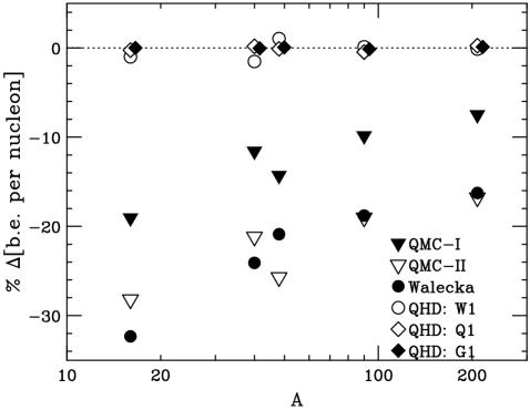
Figure 3: The deviations (in percent) between the calculated binding energy/nucleon and the empirical values for five doubly-magic nuclei. The different calculations and parameter sets are discussed in the text. For orientation, the Walecka-model results are underbound.

As a further example of the quality of the fits, and for some additional historical perspective, Fig. 3 shows the percent deviation between the calculated and empirical binding energies for the five closed-shell nuclei listed earlier. The results labeled “Walecka” are from [43], those labeled “QMC” are from recent quark–meson models of nuclear structure [50, 51, 52], and those labeled “QHD” follow from the present EFT for various parameter sets listed in Table 1. It is obvious that the modern EFT approach improves the quality of the fits by roughly two orders of magnitude and establishes a new standard of accuracy that must be attained for any modern approaches to nuclear structure to be considered viable.

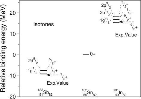
Figure 4: Binding energy of even-even ${}^{\mkern 5.0muA}_{50}$Sn isotopes calculated using the MFT of ${\cal L}_{\mathrm{QHD}}$ with parameter set G2 from Table 1 [53].

Figure 5: Calculated level spectrum of isotones of ${}^{132}_{\phantom{0}50}$Sn₈₂ differing by one proton compared with empirical results (dashed lines with arrows) [53].

Finally, to illustrate the power of the EFT approach to nuclear many-body physics, we show two recent results of Huertas [53]. The calculations use the MFT of ${\cal L}_{\mathrm{QHD}}$ with parameters fitted to closed-shell nuclei along the “valley of stability”, namely, set G2 in Table 1. The resulting self-consistent, relativistic Kohn–Sham and meson field equations are solved to calculate the properties of Sn isotopes out to doubly-magic values of $N$ and $Z$ far from stability. These results are therefore true predictions of the EFT, since no adjustments were made to previously determined parameters. Figure 5 shows the predicted binding energies of the even-even isotopes from ${}^{100}_{\phantom{0}50}$Sn to ${}^{132}_{\phantom{0}50}$Sn compared with measured experimental results. The theoretical values are accurate to better than 1% throughout. (Similar accuracy is obtained for parameter set G1; see Fig. 4 in [53].)

Figure 5 shows the predicted ground-state energies, spins, and parities of the neighboring single-particle and single-hole nuclei ${}^{133}_{\phantom{0}51}$Sb and ${}^{131}_{\phantom{0}49}$In relative to ${}^{132}_{\phantom{0}50}$Sn. The energy differences are just the chemical potentials, which should be accurately reproduced, according to the discussion of Kohn–Sham theory in Sect. 3. The excellent agreement provides compelling evidence that QHD is indeed an EFT for low-energy QCD that can be used to describe nuclear many-body physics. This recent work has been extended to semi-magic nuclei with $N=28,50,82,126\>$ and $Z=28,50,82\>$ in [54].

How can we understand the excellent accuracy of the preceding MFT results? As discussed in Sect. 3, the exact energy functional has kinetic-energy and Hartree parts (which are combined in a relativistic formulation) plus an exchange-correlation functional, which is generally a nonlocal, nonanalytic functional of the densities that contains all the other many-body, relativistic, and short-range effects [49, 55]. The basic idea behind the relativistic MFT (RMFT) is to approximate the functional using an expansion in classical meson fields (or nucleon densities) and their derivatives, based on the observation that the ratios of these quantities to the nucleon mass are small, at least up to moderate density. The parameters introduced in the expansion are fitted to experiment, and if we have a systematic way to truncate the expansion, the framework is predictive. Moreover, if the RMFT energy functional is sufficiently general, it will automatically incorporate effects beyond the Hartree approximation, such as those due to short-range physics and many-body correlations.

But why should we expect an approximate, mean-field energy functional to work so well? We observe that while the mean scalar and vector potentials $\Phi$ and $W$ are small compared to the nucleon mass, they are large on nuclear energy scales [56, 19]. Moreover, as illustrated in Dirac–Brueckner–Hartree–Fock (DBHF) calculations [45, 57, 18], the scalar and vector potentials (or self-energies) are nearly state independent and are almost equal to those obtained in the Hartree approximation. Thus the Hartree contributions to the energy functional should dominate, and an expansion of the exchange-correlation functional in terms of mean fields should be reasonable. This “Hartree dominance” also implies that it should be a good approximation to associate the single-particle Dirac eigenvalues with the empirical nuclear energy levels, at least for states near the Fermi surface [35].

We also observe that the nuclear properties of interest discussed in Sect. 1 include: 1) nuclear shape properties, such as charge radii and charge densities, 2) nuclear binding-energy systematics, and 3) single-particle properties such as level spacings and orderings, which reflect spin-orbit splittings and shell structure. Since the Kohn–Sham approach is formulated to reproduce exactly the ground-state energy and density, and the Hartree contributions are expected to dominate the Dirac single-particle potentials, these observables are indeed the ones for which meaningful comparisons with experiment should be possible.

As discussed above, an RMFT energy functional of the form in (42), extended to include low-order derivatives of the meson fields, successfully reproduces these nuclear observables with parameters of natural size (see Table 1). This justifies a truncation of the energy functional at the first few powers of the fields and their derivatives, as is evident from Fig. 1. Moreover, the full complement of parameters is underdetermined, so keeping only a subset does not preclude a realistic fit to nuclei. Both the early RMFT calculations mentioned above and the newer calculations based on chiral EFT should be interpreted within the context of this Kohn–Sham approach to DFT.

6 Analysis of Mean-Field-Theory Parameters

Although we could use meson–nucleon EFT’s as done historically, the analysis is more transparent with point-coupling theories, which contain only nucleon fields in a local Lagrangian. Because of the freedom to perform field redefinitions, a general point-coupling Lagrangian is equivalent to a general meson–nucleon Lagrangian [8, 24, 29].

An energy functional of nucleon densities can be constructed by starting with a general point-coupling effective Lagrangian, consistent with the symmetries of QCD, and by evaluating the corresponding one-loop energy functional. As discussed above, this approach approximates a general DFT functional that incorporates many-body effects beyond the Hartree level when the parameters are determined from finite-density data.

To arrive at a suitable truncation scheme, we again rely on NDA and naturalness. The two relevant mass scales are $f_{\pi}$ and $\Lambda$, and for closed-shell nuclei, the energy functional is an expansion in powers of the nucleon scalar, vector, isovector-vector, tensor, and isovector-tensor densities, which are defined as $\rho_{{\scriptstyle\rm s}}\equiv\langle{\overline{\psi}}\psi\rangle$, $\rho_{{\scriptscriptstyle\rm B}}\equiv\langle\psi^{\dagger}\psi\rangle$, $\rho_{3}\equiv{1\over 2}\langle\psi^{\dagger}\tau_{3}\psi\rangle$, ${{s}}_{i}\equiv\langle{\overline{\psi}}\sigma^{0i}\psi\rangle$, and ${{s}}_{3i}\equiv{1\over 2}\langle{\overline{\psi}}\sigma^{0i}\tau_{3}\psi\rangle$, respectively, where $\psi$ is the nucleon field.

We can then define scaled densities and their derivatives as [see (38)]

$$\widetilde{\rho}_{{\scriptstyle\rm s}}\equiv\frac{\rho_{{\scriptstyle\rm s}}}{f_{\pi}^{2}\Lambda}\ ,\quad{\widetilde{\mbox{\boldmath$\nabla$}}}\widetilde{\rho}_{{\scriptstyle\rm s}}\equiv\frac{{\mbox{\boldmath$\nabla$}}\rho_{{\scriptstyle\rm s}}}{f_{\pi}^{2}\Lambda^{2}}\ ,\quad\mathrm{etc.}$$ (44)

NDA also provides numerical estimates for the scaled densities that will allow us to estimate terms in the energy functional. For example, each additional power of $\rho_{{\scriptstyle\rm s}}$ is accompanied by a factor of $f_{\pi}^{2}\Lambda$. The ratios of scalar and vector densities to this factor at nuclear matter equilibrium density are between 1/4 and 1/7 [58], which serves as an expansion parameter. Similarly, one can anticipate good convergence for gradients of the densities, since the relevant scale for derivatives in finite nuclei is the nuclear surface thickness $\sigma$, and so the dimensionless expansion parameter is $1/\Lambda\sigma\leq 1/5$. The expansion is useful because the coefficients have been shown empirically to be natural, that is, of order unity [9, 24].

The energy functional is dominated by the isoscalar terms, but we also include the isovector and tensor terms for completeness. To nominal order $\nu=4$ (all densities and gradients count as $\nu=1$, except the three-vector tensor densities $\widetilde{{s}}$, which have $\nu\approx 2$; see also footnote 3 on p. 3), we obtain

$$E = \sum_{\alpha}^{\rm occ}\int\!{\mathrm{d}}^{3}x\;{\overline{\psi}}_{\alpha}(-i\beta\,\mbox{\boldmath$\alpha\,\cdot\,$}{\mbox{\boldmath$\nabla$}}+M)\psi_{\alpha}$$ (45)

$${}+f_{\pi}^{2}\Lambda^{2}\!\!\int\!{\mathrm{d}}^{3}x\,\bigg{\{}\widetilde{\kappa}_{2}\widetilde{\rho}_{{\scriptstyle\rm s}}^{\kern 2.0pt2}-\widetilde{\kappa}_{\rm d}({\widetilde{\mbox{\boldmath$\nabla$}}}\widetilde{\rho}_{{\scriptstyle\rm s}})^{2}+\widetilde{\kappa}_{3}\widetilde{\rho}_{{\scriptstyle\rm s}}^{\kern 2.0pt3}+\widetilde{\kappa}_{4}\widetilde{\rho}_{{\scriptstyle\rm s}}^{\kern 2.0pt4}+\widetilde{\eta}_{1}\widetilde{\rho}_{{\scriptscriptstyle\rm B}}^{\kern 2.0pt2}\widetilde{\rho}_{{\scriptstyle\rm s}}+\widetilde{\eta}_{2}\widetilde{\rho}_{{\scriptscriptstyle\rm B}}^{\kern 2.0pt2}\widetilde{\rho}_{{\scriptstyle\rm s}}^{\kern 2.0pt2}$$

$$\qquad\qquad\qquad\ {}+\widetilde{\zeta}_{2}\widetilde{\rho}_{{\scriptscriptstyle\rm B}}^{\kern 2.0pt2}-\widetilde{\zeta}_{\rm d}({\widetilde{\mbox{\boldmath$\nabla$}}}\widetilde{\rho}_{{\scriptscriptstyle\rm B}})^{2}+\widetilde{\zeta}_{4}\widetilde{\rho}_{{\scriptscriptstyle\rm B}}^{\kern 2.0pt4}-\widetilde{\alpha}_{1}\widetilde{\rho}_{{\scriptstyle\rm s}}({\widetilde{\mbox{\boldmath$\nabla$}}}\widetilde{\rho}_{{\scriptstyle\rm s}})^{2}-\widetilde{\alpha}_{2}\widetilde{\rho}_{{\scriptstyle\rm s}}({\widetilde{\mbox{\boldmath$\nabla$}}}\widetilde{\rho}_{{\scriptscriptstyle\rm B}})^{2}$$

$$\qquad\qquad\qquad\ {}+\widetilde{\xi}_{2}\widetilde{\rho}_{3}^{\kern 2.0pt2}-{\widetilde{\xi}}_{\rm d}({\widetilde{\mbox{\boldmath$\nabla$}}}\widetilde{\rho}_{3})^{2}+\widetilde{\eta}_{\rho}\widetilde{\rho}_{3}^{\kern 2.0pt2}\widetilde{\rho}_{{\scriptstyle\rm s}}+\widetilde{f}_{\rm v}{\widetilde{\mbox{\boldmath$\nabla$}}}\widetilde{\rho}_{{\scriptscriptstyle\rm B}}\mbox{\boldmath$\,\cdot\,\widetilde{{s}}$}+\widetilde{f}_{\rho}{\widetilde{\mbox{\boldmath$\nabla$}}}\widetilde{\rho}_{3}\mbox{\boldmath$\,\cdot\,{\widetilde{s}}_{{\mbox{\boldmath$\tau$}}}$}$$

$$\qquad\qquad\qquad\ {}+\ \mbox{electromagnetic\ and\ higher-order\ terms}\bigg{\}}\ ,\qquad$$

where the notation of [24] is used. The sum runs over occupied nucleon states.

In Fig. 6, the small symbols show the NDA estimates (with associated error bars) for the various energy contributions in ¹⁶O and ²⁰⁸Pb. The magnitudes of energy contributions in (45) from two representative RMF point-coupling models (i.e., two different parameter sets) are shown as larger unfilled symbols (one model on each side of the error bars). These models provide very accurate predictions of bulk nuclear properties [24]. The energy contributions are determined for each nucleus by making multiple runs while varying each parameter slightly around its optimized value, which enables us to deduce the logarithmic derivative with respect to each parameter. The filled symbols denote the sum of the values for each power of the density. The binding energy/nucleon in equilibrium nuclear matter is denoted by $\epsilon_{0}$.

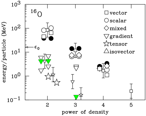
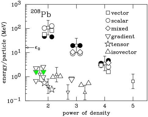
Figure 6: Contributions to the energy/particle in ¹⁶O and ²⁰⁸Pb determined by logarithmic derivatives with respect to the model parameters (see text) for two RMF point-coupling models [24]. Absolute values are shown. The filled symbols are net values. The small symbols indicate estimates based on NDA [10], with the error bars corresponding to natural coefficients from 1/2 to 2.

The two representative point-coupling models validate the isoscalar estimates (small open squares), and the resulting hierarchy of isoscalar contributions is quite clear. How far down in the hierarchy can we reliably determine contributions and their associated parameters? In Fig. 2, the impact of different truncations of RMF meson–nucleon models is shown by plotting the figure of merit against the maximum power of fields. We have also performed this test with point-coupling models, with similar conclusions. The “full” models (which include all nonredundant terms at a given order) show that one needs to go to the fourth power of the fields to get the best fits, but going further yields no improvement. Analogous behavior is found for RMF point-coupling models with powers of densities replacing powers of fields [24]. Thus contributions to the energy/particle at the level of roughly 1 MeV are at the limit of resolution. Fifth-order isoscalar contributions to the energy/particle, which are predicted to be less than 1 MeV, are simply not determined by the optimization.

The variation in coefficient values in (45) provides a measure of how well the parameters are actually determined by the data. Figure 7 shows the seven coefficients of isoscalar non-gradient terms from four point-coupling models. Note that all coefficients are natural, i.e., of order unity. However, the spread in coefficient values is significant and does not correspond well to the power-counting order. We conclude that different linear combinations of the coefficients must be considered to draw reliable conclusions about how many are determined by the data.

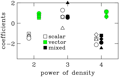
Figure 7: Coefficients for four accurately fit RMF point-coupling models from [24]. Each model is represented by a different shape, and the shading shows the type of term (scalar, vector, or mixed).

Table 2: Improved coefficients for point-coupling RMF models (Table VI of [24]).

	linear	density	deduced
coefficient	combination	scaling	value
$\widetilde{\Omega}_{1}$	$\widetilde{\kappa}_{2}+\widetilde{\zeta}_{2}$	$\rho_{+}$	$-0.51\pm 0.01$
$\widetilde{\Omega}_{3}$	$\widetilde{\kappa}_{3}+\widetilde{\eta}_{1}$	$\rho_{+}^{2}$	$+1.3\pm 0.1$
$\widetilde{\Omega}_{2}$	$\widetilde{\kappa}_{2}-\widetilde{\zeta}_{2}$	$\rho_{-}$	$-2.0\pm 0.4$
$\widetilde{\Omega}_{5}$	$\widetilde{\kappa}_{4}+\widetilde{\zeta}_{4}+\widetilde{\eta}_{2}$	$\rho_{+}^{3}$	$-2.4\pm 0.7$
$\widetilde{\Omega}_{4}$	$\widetilde{\kappa}_{3}-\widetilde{\eta}_{1}/3$	$\rho_{+}\rho_{-}$	$+0.2\pm 1.0$
$\widetilde{\Omega}_{6}$	$\widetilde{\kappa}_{4}-\widetilde{\zeta}_{4}$	$\rho_{+}^{2}\rho_{-}$	$-2.6\pm 0.8$
$\widetilde{\Omega}_{7}$	$\quad\widetilde{\kappa}_{4}+\widetilde{\zeta}_{4}-2\kern 1.0pt\widetilde{\eta}_{2}/3\quad$	$\quad\rho_{+}\rho_{-}^{2}\quad$

Can we find a more systematic power counting scheme? The similar size of the scalar density $\rho_{{\scriptstyle\rm s}}$ and the vector density $\rho_{{\scriptscriptstyle\rm B}}$ suggests that we count instead powers of $\rho_{+}\equiv(\rho_{{\scriptstyle\rm s}}+\rho_{{\scriptscriptstyle\rm B}})/2$ and $\rho_{-}\equiv(\rho_{{\scriptstyle\rm s}}-\rho_{{\scriptscriptstyle\rm B}})/2$. The corresponding “improved” coefficients are listed in Table 2 [see (45)]. The spread in these coefficients for four RMF point-coupling models from [24] is shown in Fig. 8. The terms are organized according to the powers of $\rho_{+}$ and $\rho_{-}$, with $\rho_{-}$ scaling as $\rho_{+}^{8/3}$.

The leading orders are very well determined, with a systematic increase in uncertainty. Even the sign is undetermined for the parameter $\widetilde{\Omega}_{4}$, which is shown with unfilled symbols, but the next parameter ($\widetilde{\Omega}_{6}$) appears to be reasonably well determined. Higher-order terms are not determined by the optimizations. Deduced values and uncertainties based on this sample of models are given in Table 2. We see that of the seven isoscalar non-gradient parameters in (45), four linear combinations are clearly determined by bulk nuclear observables, with probably a fifth combination as well.

Figure 8: Improved coefficients for the same four models as in Fig. 7. The “order” is determined by counting powers of $\rho_{+}$ and $\rho_{-}$.

The isovector terms appear only on the graphs for ²⁰⁸Pb. The factor $(N-Z)/2B$, which is only 10% even for Pb, severely limits the sensitivity to isovector terms (especially since the factor must appear with even powers). The magnitude of the leading isovector term ($\propto\widetilde{\xi}_{2}\widetilde{\rho}_{3}^{\kern 2.0pt2}\,$) is comparable to the fourth-order isoscalar term, which is at the limit of what can be determined reliably from fitting the binding energy. We conclude that only one isovector parameter is determined by the bulk observables. For a further discussion of the isovector terms, see [59].

The energy estimates for isoscalar, tensor terms imply that only one parameter, at best, can be determined. Higher-spin terms, which will require more gradients and have smaller average densities, are not at all constrained. The tensor terms are interesting because a fraction of the spin-orbit force can be generated by including an isoscalar, tensor coupling of the vector field to the nucleon [14]. Nevertheless, the spin-orbit potential arises predominantly from the large scalar and vector fields; attributing more than one-third of the potential to the tensor coupling produces unrealistic surface systematics [60].

Finally, gradient terms follow the same pattern in the energy: the leading term is barely above the limit of resolution. In fact, there are two isoscalar gradient terms at leading order (scalar and vector), but only their sum is well determined. The sum of the subleading-order contributions almost vanishes. We conclude that only one gradient parameter can be determined [59].

The handful of parameters that are well determined by the usual bulk nuclear observables (binding energies, charge density distributions, and spin-orbit splittings in doubly magic nuclei) can be associated with an equal number of nuclear properties and general features of RMFT’s. In particular,

1. Two isoscalar non-gradient parameters are very well determined. These correspond to the highly constrained values for the equilibrium density ($k_{\scriptscriptstyle\rm F}\approx 1.30\pm 0.01\,\mbox{fm}^{-1}$) and binding energy ($16.0\pm 0.1\,\mbox{MeV}$) of nuclear matter.

2. An additional isoscalar constraint is that $M^{*}\approx 0.61\pm 0.03$, if the isoscalar, tensor term is set to zero. This range ensures an accurate reproduction of spin-orbit splittings in finite nuclei. Small increases in $M^{*}$ without changing the splittings can be accomplished by including an isoscalar, tensor term; an analysis using a simple local-density approximation is discussed in [14].

3. A fourth isoscalar constraint comes from the nuclear matter compressibility. The constraint is much weaker, in the range of $K\approx 250\pm 50\,$MeV.

4. The possibility of a fifth isoscalar constraint has been considered by Gmuca [61], who argued that separate scalar and vector fourth-order terms were necessary to tune the density dependence of the scalar and vector parts of the baryon self-energy. This would correspond to constraining $\widetilde{\Omega}_{6}$ from Table 2. Moreover, some form of isoscalar nonlinear vector interaction is needed to soften the high-density equation of state to be consistent with observed neutron star masses [55].

5. Since only one isoscalar gradient parameter is determined, it is not useful to allow the scalar and vector masses (or their equivalents in a point-coupling theory) to vary independently. Thus it is convenient to fix the vector mass at a natural size, such as the experimental mass for the $\omega$. A scalar mass of $500\pm 20\,$MeV is then required.

6. The one isovector parameter can be fixed by the surface-corrected volume symmetry energy [62], which falls in the range $34\pm 4\,$MeV [43]. Since no isovector gradient is determined, setting the isovector, vector meson mass to the experimental $\rho$ meson mass is adequate.

To ensure a reasonable (if not optimal) description of finite nuclei, it is sufficient to reproduce the nuclear matter properties given above, but note that all calculated properties must be accurate, and the resulting parameters must be natural. One cannot justify the underlying physics of a model if it reproduces only a subset of the nuclear calibration data.

7 Weak Nuclear Currents

A desirable theory of nuclear currents should satisfy the following three criteria:

• It should use the same degrees of freedom to describe the currents and the strong-interaction dynamics.

• It should respect the same internal symmetries, both discrete and continuous, as the underlying theory of QCD.

• Its parameters can be calibrated using strong-interaction phenomena, like $\pi$N scattering and the properties of finite nuclei. This is especially important in EFT’s, as they contain all (non-redundant) interaction terms that are consistent with the underlying symmetries [63, 9].

The QHD framework described so far embodies these three desirable features.

The weak currents arise from Noether’s theorem applied directly to ${\cal L}_{\mathrm{QHD}}$ and contain the pion field to all orders. The leading-order (in $\nu$) vector and axial-vector currents are given by ($a$ is the isospin index)

$$V^{a\mu} = -i\,{{f_{\pi}^{2}}\over 4}\,{\rm Tr}\left\{{\tau}^{a}\left(U{\partial}^{\mu}U^{{\dagger}}+U^{{\dagger}}{\partial}^{\mu}U\right)\right\}+{{1}\over{4}}\,{{\overline{N\mkern 3.0mu}\mkern-3.0mu}{}}{\gamma}^{\mu}\left[{\xi}{\tau}^{a}{\xi}^{{\dagger}}+{\xi}^{{\dagger}}{\tau}^{a}{\xi}\right]N$$ (46)

$$\quad{}+{{1}\over{4}}\,g_{A}{{\overline{N\mkern 3.0mu}\mkern-3.0mu}{}}{\gamma}^{\mu}{\gamma}_{5}\left[{\xi}{\tau}^{a}{\xi}^{{\dagger}}-{\xi}^{{\dagger}}{\tau}^{a}{\xi}\right]N\ ,$$

$$A^{a\mu} = -i\,{{f_{\pi}^{2}}\over 4}\,{\rm Tr}\left\{{\tau}^{a}\left(U{\partial}^{\mu}U^{{\dagger}}-U^{{\dagger}}{\partial}^{\mu}U\right)\right\}-{{1}\over{4}}\,{{\overline{N\mkern 3.0mu}\mkern-3.0mu}{}}{\gamma}^{\mu}\left[{\xi}{\tau}^{a}{\xi}^{{\dagger}}-{\xi}^{{\dagger}}{\tau}^{a}{\xi}\right]N$$ (47)

$$\quad{}-{{1}\over{4}}\,g_{A}{{\overline{N\mkern 3.0mu}\mkern-3.0mu}{}}{\gamma}^{\mu}{\gamma}_{5}\left[{\xi}{\tau}^{a}{\xi}^{{\dagger}}+{\xi}^{{\dagger}}{\tau}^{a}{\xi}\right]N\ .$$

As discussed in [34], the Feynman rules for the lowest-order $\pi$N vertices can be determined from (3), and in the presence of an external axial-vector source, one can compute the one- and two-nucleon amplitudes for the axial-vector current. The amplitude for axial-current pion production on a single nucleon is represented by the diagrams of Fig. 9 and can be written as

$$2f_{\pi}\>M^{ab\,\mu}(\pi) = \bar{u}(p^{\prime})\left\{g^{2}_{A}\left[\not\!q\,{\gamma}_{5}\,{1\over{(\not\!p^{\mkern 2.0mu\prime}\,+\not\!q)-M}}\,{\gamma}_{5}\left({\gamma}^{\mu}-\not\!k{{{k}^{\mu}}\over{k^{2}-m_{\pi}^{2}}}\right){{{\tau}^{b}{\tau}^{a}}\over 2}\right.\right.$$ (48)

$$\qquad\qquad+\left.\left({\gamma}^{\mu}-\not\!{k}{{k^{\mu}}\over{k^{2}-m_{\pi}^{2}}}\right){\gamma}_{5}{1\over{(\not\!p\;-\not\!q)-M}}\,{\gamma}_{5}\!\not\!q\,{{{\tau}^{a}{\tau}^{b}}\over 2}\right]$$

$$\qquad\qquad+\left.i{\epsilon}^{abc}\,{{{\tau}^{c}}\over 2}\left[(\not\!k\,-\!\not\!q){{k^{\mu}}\over{k^{2}-m_{\pi}^{2}}}-2{\gamma}^{\mu}\right]\right\}u(p)\ ,$$

where $q^{\mu}$ is the outgoing four-momentum of the emitted pion, and $p^{\mu}$ and ${p^{\prime}}^{\mu}$ are the initial and final nucleon four-momenta, respectively.

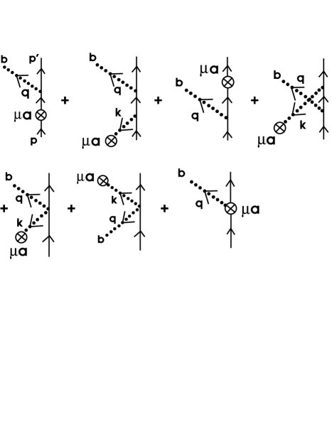
Figure 9: The amplitude for axial-current pion production on a single nucleon [Eq. (48)]. Note that momentum $k^{\mu}$ is extracted by the external source (which is denoted by $\otimes$), so that $p^{\mu}={p^{\prime}}^{\mu}+k^{\mu}+q^{\mu}$.

The two-nucleon amplitude for the axial current, to this order in $\nu$, is given in Fig. 10. It is easy to verify that this amplitude satisfies PCAC (for on-shell nucleons).

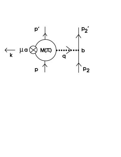
Figure 10: Two-nucleon contributions to the axial current. Here the vertex $M(\pi)$ [Eq. (48)] represents all possible ways that the external source can couple to the left-hand nucleon line (to the order we are working), as illustrated in Fig. 9. There are also contributions from the right-hand nucleon line, as well as exchange terms.

One can also determine the vector and axial-vector currents arising from the $\nu=3$ and $\nu=4$ terms in the QHD Lagrangian (3). These additional contributions take the form

$$\delta V^{a\mu} = {-{i{\kappa}_{\pi}}\over{2M}}\,{{\overline{N\mkern 3.0mu}\mkern-3.0mu}{}}{\sigma}^{\mu\nu}\left[{\xi}^{{\dagger}}{\tau}^{a}\xi-\xi{\tau}^{a}{\xi}^{{\dagger}},\>a_{\nu}\right]N-{{2{\beta}_{\pi}}\over{M}}\,{{\overline{N\mkern 3.0mu}\mkern-3.0mu}{}}N\,{\rm Tr}\left[({\xi}^{{\dagger}}{\tau}^{a}\xi-\xi{\tau}^{a}{\xi}^{{\dagger}})\,a^{\mu}\right]$$ (49)

$$\quad{}-{\epsilon}^{abc}{\rho}^{b}_{\nu}\left\{{{f_{\rho}g_{\rho}}\over{4M}}\,{{\overline{N\mkern 3.0mu}\mkern-3.0mu}{}}{\sigma}^{\mu\nu}{\tau}^{c}N+\left({\partial}^{\mu}{\rho}^{\nu}_{c}-{\partial}^{\nu}{\rho}^{\mu}_{c}\right)+O({\pi}^{2})\right\}$$

and

$$\delta A^{a\mu} = {-{i{\kappa}_{\pi}}\over{2M}}\,{{\overline{N\mkern 3.0mu}\mkern-3.0mu}{}}{\sigma}^{\mu\nu}\left[{\xi}^{{\dagger}}{\tau}^{a}\xi+\xi{\tau}^{a}{\xi}^{{\dagger}},\>a_{\nu}\right]N-{{2{\beta}_{\pi}}\over{M}}\,{{\overline{N\mkern 3.0mu}\mkern-3.0mu}{}}N\,{\rm Tr}\left[({\xi}^{{\dagger}}{\tau}^{a}\xi+\xi{\tau}^{a}{\xi}^{{\dagger}})\,a^{\mu}\right]$$ (50)

$$\quad{}+\left\{g_{\rho\pi\pi}\,{{2f_{\pi}}\over{m_{\rho}^{2}}}\,{\epsilon}^{abc}\,{\partial}_{\nu}{\pi}^{b}\left({\partial}^{\mu}{\rho}^{\nu}_{c}-{\partial}^{\nu}{\rho}^{\mu}_{c}\right)+O(\rho^{2}\pi,\,\rho\pi^{3})\right\}\ .$$

The terms proportional to $\kappa_{\pi}$ and $\beta_{\pi}$ produce the two-nucleon amplitudes shown in Fig. 11. The corresponding amplitudes involving rho meson exchange are illustrated in Fig. 12, and there are also amplitudes with isoscalar scalar and vector meson exchange that resemble the first two diagrams in this figure. Analytical expressions for all of these two-nucleon amplitudes are given in [34].

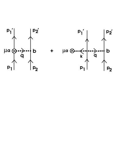
Figure 11: Two-nucleon, axial-current amplitudes originating from the $\nu=3$ pion–nucleon terms in the effective Lagrangian. There is one pair of diagrams proportional to $\kappa_{\pi}$ and another pair proportional to $\beta_{\pi}$.

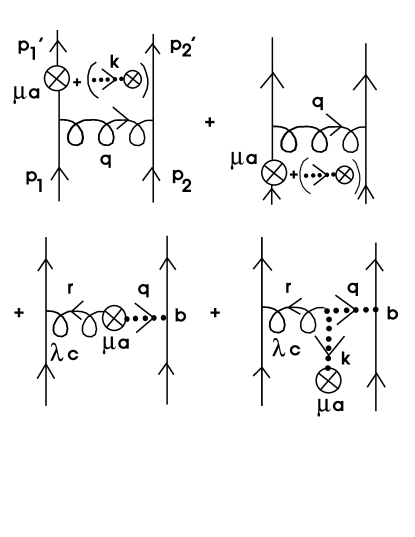
Figure 12: Two-nucleon, axial-current amplitudes containing rho meson exchange. The notation in the first two diagrams implies that the external source can couple to the nucleon line in two ways, as in Fig. 11.

The scattering amplitudes constructed from the currents listed above satisfy CVC, PCAC (when $m_{\pi}\not=0$), and the Goldberger–Treiman relation (with $g_{A}\not=1$) automatically. Moreover, the chiral charges $Q^{a}$ and $Q_{5}^{a}$ derived from these currents satisfy the familiar chiral charge algebra to all orders in the pion field [34]. In [64], these currents are used to study beta decay in ^131,133Sn.

8 Summary

In this work, I discussed recent progress in Lorentz-covariant quantum field theories of the nuclear many-body problem, often called quantum hadrodynamics (QHD). QHD is a local, nonrenormalizable, effective Lagrangian field theory with baryons and mesons as the generalized coordinates (fields). An effective Lagrangian consists of known long-range interactions constrained by symmetries and a complete, non-redundant set of short-range interactions. By simply looking at the spectra of massive nuclei, it is obvious that some relativistic effects must be important in nuclei; thus, it is most convenient to use a Lorentz-covariant theory.

The effective field theory studied here contains nucleons, pions, isoscalar scalar ($\sigma$) and vector ($\omega$) fields, and isovector vector ($\rho$) fields. The heavy mesons are introduced as collective, effective degrees of freedom to simplify the description of the medium- and short-range nucleon–nucleon interaction and to conveniently parametrize ground-state expectation values of nucleon bilinears, which are important for the description of bulk nuclear properties. The QHD theory exhibits a nonlinear realization of spontaneously broken $\mathrm{SU(2)}_{L}\times\mathrm{SU(2)}_{R}$ chiral symmetry and has three desirable features: it uses the same degrees of freedom to describe the nuclear currents and the strong-interaction dynamics, it respects the symmetries of the underlying theory of QCD, and its parameters can be calibrated using strong-interaction phenomena. Moreover, the electromagnetic structure of the nucleon can be included straightforwardly in a derivative expansion of the fields.

Although the QHD Lagrangian in principle contains an infinite number of terms, naive dimensional analysis and naturalness allow one to identify suitable expansion parameters and to estimate the sizes of various terms in the Lagrangian. Thus, for any desired accuracy, the Lagrangian can be truncated to a finite number of terms. In particular, for normal nuclear systems, it is possible to expand the QHD effective Lagrangian systematically in powers of the meson fields (and their derivatives) and to truncate the expansion reliably after the first few orders.

Using density functional theory, I showed that the mean-field approximation produces an energy functional whose parameters can be determined by fitting bulk and single-particle properties of nuclei. The framework of Kohn–Sham theory allows the ground state to be constructed from (quasi)particle orbitals with unit occupation number. Since the mean-field energy functional is a good approximation to the exact energy functional over the relevant range of density, it is possible to reproduce nuclear densities, binding energies, and single-particle spectra near the Fermi surface very accurately. Because the parameters are fitted to nuclear properties, the energy functional implicitly contains effects that go beyond a simple Hartree approximation, such as short-range physics, hadron substructure, and many-body correlations.

The numerical parameters of QHD were studied using an effective, point-coupling Lagrangian that contains nucleon fields only. Because of the freedom to redefine the fields (or coordinates), a general point-coupling theory is equivalent to a general baryon–meson theory. By examining the contributions to the energy/nucleon in doubly magic nuclei, it was found that only a small number of parameters (roughly seven) can be calibrated by the nuclear data input. New ways to calibrate additional parameters will play an important role in the construction of the next generation of QHD Lagrangians. Finally, the weak vector and axial-vector currents, and the corresponding two-nucleon, axial-current amplitudes, were discussed in the QHD framework.

Nuclear physics is the study of strongly interacting hadronic matter, and the only consistent theoretical framework we have for describing such a relativistic, interacting, quantum-mechanical, many-body system is relativistic quantum field theory based on a local Lagrangian density. Although QCD of quarks and gluons provides the basic underlying theory, Lagrangians comprised of hadronic degrees of freedom (QHD) provide the most efficient description of the physics in the strong-coupling domain. In the modern effective field theory perspective of QCD, one incorporates only the underlying symmetries of QCD into the QHD Lagrangian. By interpreting the mean-field approximation in the context of density functional theory, one can understand the numerous successes of the QHD description of nuclear properties. Nevertheless, finding an efficient, tractable, nonperturbative way to match the QCD Lagrangian to the long-range, strong-coupling, effective field theory of QHD is still a major goal for the future.

References

- [1] A. L. Fetter and J. D. Walecka: Quantum Theory of Many-Particle Systems (McGraw–Hill, New York 1971), chaps. 11 and 15. Reprinted by Dover Publications, Mineola, New York (2003).
- [2] J. D. Walecka: Theoretical Nuclear and Subnuclear Physics (Oxford Univ. Press, New York 1995); second ed. (World Scientific, Singapore 2004), part 1.
- [3] B. D. Serot and J. D. Walecka: Adv. Nucl. Phys. 16, 1 (1986), and references therein.
- [4] J. D. Bjorken and S. D. Drell: Relativistic Quantum Mechanics (McGraw–Hill, New York 1964, 1998), Fig. 4–2.
- [5] M. G. Mayer and J. H. D. Jensen: Elementary Theory of Nuclear Shell Structure (Wiley, New York 1955), p. 58.
- [6] J. D. Walecka: Ann. Phys. (New York) 83, 491 (1974).
- [7] B. D. Serot: Rep. Prog. Phys. 55, 1855 (1992).
- [8] R. J. Furnstahl, B. D. Serot, and H.-B. Tang: Nucl. Phys. A615, 441 (1997); A640, 505 (1998) (E).
- [9] B. D. Serot and J. D. Walecka: Int. J. Mod. Phys. E 6, 515 (1997), and references therein.
- [10] R. J. Furnstahl and B. D. Serot: Nucl. Phys. A671, 447 (2000).
- [11] R. J. Furnstahl and B. D. Serot: Nucl. Phys. A673, 298 (2000).
- [12] R. J. Furnstahl and B. D. Serot: Comments Mod. Phys. 2, A23 (2000).
- [13] B. D. Serot and J. D. Walecka, in: 150 Years of Quantum Many-Body Theory, ed. by R. F. Bishop, K. A. Gernoth, and N. R. Walet (World Scientific, Singapore 2001), pp. 203–211.
- [14] R. J. Furnstahl, J. J. Rusnak, and B. D. Serot: Nucl. Phys. A632, 607 (1998).
- [15] T. D. Cohen, R. J. Furnstahl, and D. K. Griegel: Phys. Rev. Lett. 67, 961 (1991).
- [16] R. J. Furnstahl, D. K. Griegel, and T. D. Cohen: Phys. Rev. C 46, 1507 (1992).
- [17] B. C. Clark, S. Hama, R. L. Mercer, L. Ray, and B. D. Serot: Phys. Rev. Lett. 50, 1644 (1983).
- [18] R. Machleidt: Adv. Nucl. Phys. 19, 189 (1989).
- [19] R. J. Furnstahl, H.-B. Tang, and B. D. Serot: Phys. Rev. C 52, 1368 (1995).
- [20] H.-B. Tang: hep-ph/9607436, unpublished.
- [21] P. J. Ellis and H.-B. Tang: Phys. Rev. C 57, 3356 (1998).
- [22] T. Becher and H. Leutwyler: Eur. Phys. J. C 9, 643 (1999).
- [23] B. A. Nikolaus, T. Hoch, and D. G. Madland: Phys. Rev. C 46, 1757 (1992).
- [24] J. J. Rusnak and R. J. Furnstahl: Nucl. Phys. A627, 495 (1997).
- [25] H.-B. Tang and P. J. Ellis: Phys. Lett. B387, 9 (1996).
- [26] H. Georgi and A. Manohar: Nucl. Phys. B234, 189 (1984).
- [27] H. Georgi: Phys. Lett. B298, 187 (1993).
- [28] R. J. Furnstahl, B. D. Serot, and H.-B. Tang: Nucl. Phys. A598, 539 (1996).
- [29] R. J. Furnstahl, H.-W. Hammer, and N. Tirfessa: Nucl. Phys. A689, 846 (2001).
- [30] B. D. Serot: Phys. Lett. 86B, 146 (1979); 87B, 403 (1979) (E).
- [31] S. Coleman, J. Wess, and B. Zumino: Phys. Rev. 177, 2239 (1969).
- [32] C. G. Callan, Jr., S. Coleman, J. Wess, and B. Zumino: Phys. Rev. 177, 2247 (1969).
- [33] U. van Kolck: Prog. Part. Nucl. Phys. 43, 337 (1999).
- [34] S. M. Ananyan, B. D. Serot, and J. D. Walecka: Phys. Rev. C 66, 055502 (2002).
- [35] R. M. Dreizler and E. K. U. Gross: Density Functional Theory (Springer, Berlin Heidelberg New York 1990).
- [36] L. H. Thomas: Proc. Cambridge Phil. Soc. 23, 542 (1927).
- [37] E. Fermi: Z. Phys. 48, 73 (1928).
- [38] N. Argaman and G. Makov: Am. J. Phys. 68, 69 (2000).
- [39] W. Kohn: Rev. Mod. Phys. 71, 1253 (1999).
- [40] W. Kohn and L. J. Sham: Phys. Rev. A140, 1133 (1965).
- [41] A. H. MacDonald and S. H. Vosko: J. Phys. C 12, 2977 (1979).
- [42] C. O. Almbladh and U. von Barth: Phys. Rev. B 31, 3231 (1985).
- [43] C. J. Horowitz and B. D. Serot: Nucl. Phys. A368, 503 (1981).
- [44] P. Ring: Prog. Part. Nucl. Phys. 37, 193 (1996), and references therein.
- [45] C. J. Horowitz and B. D. Serot: Nucl. Phys. A464, 613 (1987); A473, 760 (1987) (E).
- [46] J. L. Friar, D. G. Madland, and B. W. Lynn: Phys. Rev. C 53, 3085 (1996).
- [47] S. Weinberg: Phys. Lett. B251, 288 (1990).
- [48] W. H. Furry: Phys. Rev. 50, 784 (1936).
- [49] R. J. Furnstahl, C. E. Price, and G. E. Walker: Phys. Rev. C 36, 2590 (1987).
- [50] K. Saito and A. W. Thomas: Phys. Lett. B327, 9 (1994).
- [51] K. Saito, K. Tsushima, and A. W. Thomas: Nucl. Phys. A609, 339 (1996).
- [52] K. Saito, K. Tsushima, and A. W. Thomas: Phys. Rev. C 55, 2637 (1997).
- [53] M. A. Huertas: Phys. Rev. C 66, 024318 (2002); 67, 019901 (2003) (E).
- [54] M. A. Huertas: Acta Phys. Polon. B 35, 837 (2004).
- [55] H. Müller and B. D. Serot: Nucl. Phys. A606, 508 (1996).
- [56] A. R. Bodmer: Nucl. Phys. A526, 703 (1991).
- [57] B. ter Haar and R. Malfliet: Phys. Rep. 149, 207 (1987).
- [58] J. L. Friar: Few Body Sys. 99, 1 (1996).
- [59] R. J. Furnstahl: Nucl. Phys. A706, 85 (2002).
- [60] G. Hua, T. v. Chossy, and W. Stocker: Phys. Rev. C 61, 014307 (2000).
- [61] S. Gmuca: Z. Phys. A342, 387 (1992); Nucl. Phys. A547, 447 (1992).
- [62] P. A. Seeger and W. M. Howard: Nucl. Phys. A238, 491 (1975).
- [63] S. Weinberg: The Quantum Theory of Fields, vol. I: Foundations (Cambridge Univ. Press, Cambridge, UK 1995).
- [64] M. A. Huertas: Acta Phys. Polon. B 34, 4269 (2003).