Fluctuations from Thermalization at RHIC

Abstract

The centrality dependence of dynamic fluctuations of the transverse momentum and the net charge can signal the approach to local thermal equilibrium in nuclear collisions. I explore this signal by comparing transport-theory calculations to STAR and PHENIX data at a range of energies. In particular, I find that this model can describe PHENIX data on the dependence of fluctuations on the $p_{t}$ range in which they are measured.

1 Introduction

Measurements of the event-by-event fluctuations of the mean transverse momentum exhibit substantial dynamic contributions [1]. PHENIX and STAR data for Au+Au collisions show that such fluctuations increase as centrality increases [2, 3]. In addition, the measured dynamic net-charge fluctuations may show an analogous behavior [3]. Importantly, the event-averaged transverse momentum $\langle p_{t}\rangle$ – a quantity unaffected by fluctuations – exhibits a strikingly similar behavior [4, 5].

I ask whether the onset of local thermal equilibrium can explain the common centrality dependence of these quantities. I seek a nonequilibrium explanation because the strongest observed changes occur in peripheral collisions, where equilibrium is not expected. This is important because similar behavior can accompany the hadronization of quark-gluon plasma, but only if the matter is thermalized [6]. My discussion follows the transport-theory formulation in ref. [7]. Here, I present work in progress confronting new measurements of the variation of $p_{t}$ fluctuations as a function of the observed $p_{t}$ region [2]; see fig. 2.

Dynamic fluctuations are generally determined from the measured fluctuations by subtracting the statistical value expected, e.g., in equilibrium [8]. For particles of momenta $\mathbf{p}_{1}$ and $\mathbf{p}_{2}$, dynamic multiplicity fluctuations are characterized by the robust variance

$$R_{AA}={{\langle N^{2}\rangle-\langle N\rangle^{2}-\langle N\rangle}\over{\langle N\rangle^{2}}}={{1}\over{\langle N\rangle^{2}}}\int\!d\mathbf{p}_{1}d\mathbf{p}_{2}\,r(\mathbf{p}_{1},\mathbf{p}_{2}),$$ (1)

where $\langle\cdots\rangle$ is the event average. This quantity depends only on the two-body correlation function $r(\mathbf{p}_{1},\mathbf{p}_{2})=N(\mathbf{p}_{1},\mathbf{p}_{2})-N(\mathbf{p}_{1})N(\mathbf{p}_{2})$, see also [9]. It is obtained from the multiplicity variance by subtracting its Poisson value $\langle N\rangle$. To make $R_{AA}$ robust, we divide by $\langle N\rangle^{2}$ to minimized the effect of experimental efficiency [8]. For dynamic $p_{t}$ fluctuations one similarly finds

$$\langle\delta p_{t1}\delta p_{t2}\rangle=\int\!d\mathbf{p}_{1}d\mathbf{p}_{2}\,{{r(\mathbf{p}_{1},\mathbf{p}_{2})}\over{\langle N(N-1)\rangle}}\delta p_{t1}\delta p_{t2},$$ (2)

where $\delta p_{ti}=p_{ti}-\langle p_{t}\rangle$; STAR measures this observable. The observable measured by PHENIX satisfies $F_{p_{t}}\approx N\langle\delta p_{t1}\delta p_{t2}\rangle/2\sigma^{2}$ when dynamic fluctuations are small compared to statistical fluctuations $\sigma^{2}=\langle p_{t}^{2}\rangle-\langle p_{t}\rangle^{2}$.

Thermalization occurs as scattering drives the phase space distribution within a small fluid cell toward a Boltzmann distribution, which varies in space through the temperature $T(\mathbf{x},t)$. The time scale for this process is the relaxation time $\nu^{-1}$. In contrast, density differences between fluid cells must be dispersed by transport from cell to cell. The time needed for diffusion to disperse a dense fluid “clump” of size $L\sim(|\nabla n|/n)^{-1}$ is $t_{\rm d}\sim\nu L^{2}/v_{\rm th}^{2}$, where $v_{\rm th}\sim 1$ is the thermal speed of particles. This time can be much larger than $\nu^{-1}$ for a sufficiently large clumps. Global equilibrium, in which the system is uniform, can be only obtained for $t\gg t_{\rm d}$. However, the rapid expansion of the collision system prevents inhomogeneity from being dispersed prior to freeze out.

Dynamic fluctuations depend on the number of independent particle “sources.” This number changes as the system evolves. Initially, these sources are the independent strings formed as the nuclei collide. The system is highly correlated along the string, but is initially uncorrelated in the transverse plane. As local equilibration proceeds, the clumps become the sources. The fluctuations at this stage depend on number of clumps as determined by the clump size, i.e., the correlation length in the fluid. Dynamic fluctuations would eventually vanish if the system were to reach global equilibrium, where statistical fluctuations would be determined by the total number of particles.

2 Mean $p_{t}$ and its Fluctuations

Fig. 1.: Mean $p_{t}$ (left) and its fluctuations (right) vs. centrality with data [5, 2]. Preliminary $\Lambda$ data is from [4]. Centrality in all figures is determined by the number of participants relative to the b=0 value.

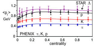
In [7] I use the Boltzmann transport equation to show that thermalization alters the average transverse momentum following

$$\langle p_{t}\rangle=\langle p_{t}\rangle_{o}S+\langle p_{t}\rangle_{e}(1-S),$$ (3)

where $S\equiv e^{-{\mathcal{N}}}$ is the probability that a particle escapes the collision volume without scattering. The initial value $\langle p_{t}\rangle_{o}$ is determined by the particle production mechanism. If the number of collisions $\mathcal{N}$ is small, $S\approx 1-\mathcal{N}$ implies the random-walk-like increase of $\langle p_{t}\rangle$ relative to $\langle p_{t}\rangle_{o}$. For a longer-lived system, energy conservation limits $\langle p_{t}\rangle$ to a local equilibrium value $\langle p_{t}\rangle_{e}$ fixed by the temperature.

As centrality is increased, the system lifetime increases, eventually to a point where local equilibrium is reached. Correspondingly, the survival probability $S$ in (3) decreases with increasing centrality. The average $p_{t}$ peaks for impact parameters near the point where equilibrium is established. The behavior in events beyond that centrality depends on how the subsequent hydrodynamic evolution changes $\langle p_{t}\rangle_{e}$ as the lifetime increases. Systems formed in the most central collisions experience a cooling that reduces (3) with proper time $\tau$ as $\langle p_{t}\rangle_{e}\propto\tau^{-\gamma}$ [7].

Thermalization can explain the behavior in fig. 1. The survival probability is $S=\exp\{-\int_{\tau_{0}}^{\tau_{F}}\nu(\tau)d\tau\}\approx(\tau_{0}/\tau_{F})^{\alpha}$, where $\nu=\langle\sigma v_{\rm rel}\rangle n(\tau)$ for $\sigma$ the scattering cross section, $v_{\rm rel}$ the relative velocity, and $\tau_{0,F}$ the formation and freeze out times. Longitudinal expansion implies $n(\tau)\propto\tau^{-1}$, yielding the power law with $\alpha=\nu_{0}\tau_{0}$. To fit the measured centrality dependence, I assume $\alpha=4$ and $\gamma=0.15$ in central collisions, and parameterize $S(N_{\rm part})$ by taking $\alpha\propto N_{\rm part}^{1/2}$ and $\tau_{F}-\tau_{0}\propto N_{\rm part}$, where $N_{\rm part}$ is the number of participants. I take the same $\alpha$ for all species, as appropriate for parton scattering.

Dynamic fluctuations depend on two-body correlations and, correspondingly, are quadratic in the survival probability. In [7] I add Langevin noise terms to the Boltzmann equation to describe the fluctuations of the phase space distribution. A simple limit is obtained when the initial correlations are independent of those near local equilibrium, $\langle\delta p_{t1}\delta p_{t2}\rangle=\langle\delta p_{t1}\delta p_{t2}\rangle_{o}S^{2}+\langle\delta p_{t1}\delta p_{t2}\rangle_{e}(1-S)^{2}$; this form was used in [7]. Alternatively, if the initial correlations are not far from the local equilibrium value, I find

$$\langle\delta p_{t1}\delta p_{t2}\rangle=\langle\delta p_{t1}\delta p_{t2}\rangle_{o}S^{2}+\langle\delta p_{t1}\delta p_{t2}\rangle_{e}(1-S^{2}).$$ (4)

Here I use (4), which provides somewhat better agreement with the latest STAR data in the peripheral region where thermalization is incomplete (and my model assumptions most applicable). As before, the initial quantity $\langle\delta p_{t1}\delta p_{t2}\rangle_{o}$ is determined by the particle production mechanism, while $\langle\delta p_{t1}\delta p_{t2}\rangle_{e}$ describes the system near local equilibrium.

To estimate $\langle\delta p_{t1}\delta p_{t2}\rangle_{o}$ for nuclear collisions, I apply the wounded nucleon model to describe the soft production that dominates $\langle p_{t}\rangle$ and $\langle\delta p_{t1}\delta p_{t2}\rangle$, to find

$$\langle\delta p_{t1}\delta p_{t2}\rangle_{o}={{2\langle\delta p_{t1}\delta p_{t2}\rangle_{pp}}\over{N_{\rm part}}}\left({{1+R_{pp}}\over{1+R_{AA}}}\right)$$ (5)

[7]. The pre-factor is expected because (2) measures relative fluctuations and, therefore, should scale as $N_{\rm part}^{-1}$. The term in parentheses accounts for the normalization of (2) to $\langle N(N-1)\rangle$; $R_{AA}$ scales as $N_{\rm part}^{-1}$ [8]. ISR measurements imply $\langle\delta p_{t1}\delta p_{t2}\rangle_{pp}/\langle p_{t}\rangle_{pp}^{2}\approx 0.015$. I use HIJING to estimate $R_{pp}$ and $R_{AA}$.

Near local equilibrium, spatial correlations occur because the fluid is inhomogeneous – it is more likely to find particles near a dense clump. These spatial correlations fully determine the momentum correlations since the distribution at each point is thermal. The mean $p_{t}$ at each point is proportional to the temperature $T(\mathbf{x})$, so that $\langle\delta p_{t1}\delta p_{t2}\rangle_{e}\sim\int r(\mathbf{x}_{1},\mathbf{x}_{2}){\delta T}(\mathbf{x}_{1}){\delta T}(\mathbf{x}_{2})$, where $r(\mathbf{x}_{1},\mathbf{x}_{2})$ is the spatial correlation function, $\delta T=T-\overline{T}$, and $\overline{T}$ is a density-weighted average. I take $n$ ($\propto T^{3}$) and $r$ to be Gaussian with the transverse widths $R_{t}$ and $\xi_{t}$, respectively the system radius and correlation length. In [7] I obtain

$$\langle\delta p_{t1}\delta p_{t2}\rangle_{e}=F{{\langle p_{t}\rangle^{2}R_{AA}}\over{1+R_{AA}}}$$ (6)

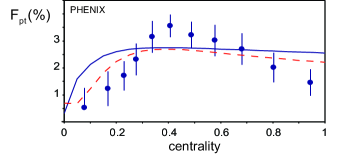
where $R_{AA}$ is given by (1) [7]. The dimensionless quantity $F$ depends on $\xi_{t}/R_{t}$. I compute $F$ assuming $R_{t}\propto N_{\rm part}^{1/2}$; $F=0.046$ for $\xi_{t}/R_{t}=1/6$. I again use HIJING to estimate $R_{AA}$. Calculations are compared to PHENIX data in fig. 1 (right), and agree within the large uncertainties.

Fig. 2.: Dynamic $p_{t}$ fluctuations with PHENIX data for central Au+Au as a function of the acceptance 0.2 GeV $<p_{t}<p_{t,\,{\rm max}}$ [2].

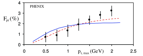
PHENIX also reports $F_{p_{t}}$ in the acceptance region $0.2$ GeV $<p_{t}<p_{t,\,{\rm max}}$ as a function of $p_{t,\,{\rm max}}$, with the intent of identifying the role of jets in producing fluctuations [2]. To exhibit the acceptance dependence of $F_{p_{t}}$, I use (1) and (2) to estimate $\langle\delta p_{t1}\delta p_{t2}\rangle\approx\sigma^{2}R_{AA}$, where $\sigma^{2}=\langle p_{t}^{2}\rangle-\langle p_{t}\rangle^{2}$. This result is exact for short range transverse correlations. I then write the observed quantity $F_{p_{t},\,{\rm obs}}\approx(\langle N\rangle\langle\delta p_{t1}\delta p_{t2}\rangle/2\sigma^{2})_{\rm obs}\propto\langle N\rangle_{\rm obs}R_{AA,\,{\rm obs}}$. The observed multiplicity grows strongly as $p_{t,\,{\rm max}}$ is increased, since $\langle N\rangle_{\rm obs}$ is the integral of the $p_{t}$ distribution over the acceptance. To determine the $p_{t,\,{\rm max}}$ dependence of $R_{AA,\,{\rm obs}}$, let the probability that an individual particle falls in the acceptance region be $a$. The average number of detected particles is $\langle N\rangle_{\rm obs}=a\langle N\rangle$. For a binomial distribution, one has $\langle N^{2}\rangle_{\rm obs}=a^{2}\langle N^{2}\rangle+a(1-a)\langle N\rangle$, so that (1) implies $R_{AA,\,{\rm obs}}=R_{AA}$, the value for full acceptance. It follows that

$$F_{p_{t},\,{\rm obs}}\approx F_{p_{t}}{{\langle N\rangle_{\rm obs}}\over{\langle N\rangle}}$$ (7)

where $F_{p_{t}}$ and $\langle N\rangle$ are for full acceptance. I emphasize that this estimate only includes trivial acceptance effects. I omit contributions to the $p_{t,\,{\rm max}}$ dependence from the onset of jets, as well as changes in the correlations due to restricting $p_{t}$.

The estimated $p_{t,\,{\rm max}}$ dependence of $F_{p_{t}}$ accounts for the data in fig. 2. The solid curve is computed for $\langle N\rangle_{\rm obs}\propto 1-e^{-p_{t,\,{\rm max}}/T}(1+{{p_{t,\,{\rm max}}}/{T}})$ for a thermal distribution at the freeze out temperature obtained from the measured $\langle p_{t}\rangle$; the dashed curve for $T=600$ MeV is included to show the $T$ dependence. These curves are arbitrarily normalized, since my computed values in fig. 1 fall above the most central PHENIX data (but below STAR, see fig. 3). Jets may account for the discrepancy at the highest $p_{t,\,{\rm max}}$.

The agreement in figs. 1 and 2 is excellent – and therefore somewhat puzzling – since I have neglected collective flow [10]. Flow must contribute to fluctuations at some level. However, thermalization and radial flow are manifestations of multiple scattering in different regimes; the flow velocity is uniquely defined only when local equilibrium is established. Both effects enhance $p_{t}$, so that the flow contribution may be partly concealed by my parameter choices.

Preliminary STAR $p_{t}$ and net charge fluctuation data in fig. 3 show fluctuations at 20, 130 and 200 GeV beam energies. To compute this energy dependence, I assume $\alpha\propto N$, $R_{AA}\propto N^{-1}$ and take $N$ from data. The $p_{t}$ fluctuation data show a tantalizing similarity to the calculations, although the experimental uncertainty must be reduced to firmly establish the behavior at high multiplicity.

Fig. 3.: Dynamic $p_{t}$ (left) and net charge (right) fluctuations with STAR data [3]. The curves and data are for beam energies 20, 130, and 200 GeV. The behavior of $\nu_{\rm dyn}$ appears inverted because this quantity is negative.

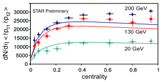
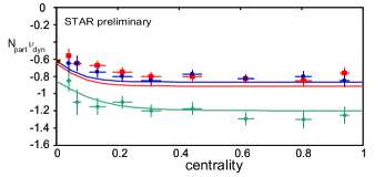
Net charge fluctuations in fig. 3 (right) are characterized by $\nu_{dyn}=R^{++}+R^{--}-2R^{+-}$ for $R^{ab}$ given by (1) [12]. I therefore expect $\nu_{dyn}$ to satisfy $\nu_{dyn}=\nu_{o}S^{2}+\nu_{e}(1-S^{2})$. I use pp data to fix $\nu_{0}$ and compute $\nu_{e}/\nu_{0}$ assuming the longitudinal narrowing of the correlation length seen in balance function data [11]. The agreement of in-progress calculations with preliminary data [3, 12] is encouraging.

Deviations of the calculated fluctuations from data in central collisions at the highest energies are expected due to flow [10] and jets [1]. Such deviations may be seen in fig. 3. Nevertheless, I stress that hard scattering effects – including jet quenching – are incorporated in my calculations via the HIJING $R_{AA}$ in (6). HIJING alone does not describe the data discussed here [11].

Thermalization is consistent with the acceptance dependence in fig. 2. I surmise that (7) holds for a range of models, since my argument was rather general. That said, precise measurements may yet reveal jet and flow contributions [1, 10]. I find that $\nu_{\rm dyn}$ and $\langle\delta p_{t1}\delta p_{t2}\rangle/\langle p_{t}\rangle^{2}$ minimize trivial acceptance effects and are correspondingly less ambiguous.