Incorporation of three–nucleon force in the effective interaction hyperspherical harmonic approach

Abstract

It is shown how a bare three–nucleon force is incorporated into the formalism of the effective interaction approach for hyperspherical harmonics. As a practical example we calculate the ground state properties of ³H and ³He using the Argonne V18 nucleon–nucleon potential and the Urbana IX three–nucleon force. A very good convergence of binding energies and matter radii is obtained. We also find a very good agreement of our results compared to other high precision calculations.

I Introduction

It is well known that the binding energies of the three–body nuclei cannot be obtained with NN forces only and thus also three–nucleon (3N) forces have to be included. This makes realistic calculations for systems with more than two nucleons more difficult. Nonetheless such calculations have been carried out in three– and four–nucleon systems by various groups using different theoretical methods: Green Function Monte Carlo GFMC (also for $A>4$) as well as hyperspherical harmonics (HH) expansions and Faddeev techniques (see e.g. ELOT ; ELOT2 ; BoPi ; Nogga ). It would be very desirable to extend such an exact treatment of 3N forces to methods based on effective interaction approaches, since they are very suitable to treat also systems with $A>4$. In case of the effective interaction approach within the No Core Shell Model (NCSM) such calculations have already been performed. Rather good results have been obtained NCSM , though without reaching a convergence as excellent as in other methods. For the effective interaction hyperspherical harmonics (EIHH) technique EIHH1 an inclusion of bare 3N forces had not yet been accomplished. In fact the aim of the present paper is to show how such a 3N force is incorporated in the EIHH formalism. A further aim is to check whether a comparably good convergence as with methods, which do not use effective interaction approaches, can be reached. To this end results of a calculation of three–nucleon groundstate properties using the AV18 NN potential AV18 and the UrbIX 3N force UrbIX are presented.

The paper is organized as follows. In section II the EIHH method is briefly outlined, while the incorporation of the 3N force in the EIHH method is described in section III. Results for the three–nucleon groundstate properties are discussed in section IV. Details for the calculation of the 3N force matrix elements are given in the Appendix.

II Brief outline of the EIHH method

To apply an effective interaction method to an $A$–body Hamiltonian of the form

$$H^{[A]}=H_{0}+V$$ (1)

one divides the Hilbert space of $H^{[A]}$ into a model space P and a residual space Q with eigenprojectors $P$ and $Q$ of $H_{0}$. The Hamiltonian $H^{[A]}$ is then replaced by an effective model–space Hamiltonian

$$H^{[A]eff}=PH_{0}P+PV^{[A]eff}P\;$$ (2)

that by construction has the same energy levels as the low–lying states of $H^{[A]}$. To find $V^{[A]eff}$, however, is as difficult as seeking the full–space solutions. In the EIHH method, as in the NCSM method, one approximates $V^{[A]eff}$ in such a way that it coincides with $V$ for P$\longrightarrow 1$, so that an enlargement of P leads to a convergence of the eigenenergies to the true values.

Considering a Hamiltonian that contains besides the kinetic energy $T$ only a two–body interaction $v^{[2]}_{ij}$,

$$H^{[A]}=T+\sum_{i<j}^{A}v^{[2]}_{ij}\,,$$ (3)

one can rewrite $H$ in the hyperspherical formalism as

$$H^{[A]}=T_{\rho}+T_{K}(\rho)+V^{[A]}(\rho,\Omega_{A})\,,$$ (4)

where

$$V^{[A]}(\rho,\Omega_{A})\equiv\sum_{i<j}^{A}v^{[2]}_{ij}\,,\,\,\,\,\,T_{\rho}=-\frac{1}{2m}\Delta_{\rho}\,,\,\,\,\,\,T_{K}(\rho)=\frac{1}{2m}\frac{\hat{K}_{A}^{2}}{\rho^{2}}$$ (5)

are the bare two–body potential and the hyperradial/hypercentrifugal kinetic energies, respectively, $m$ is the particle mass, $\hat{K}_{A}$ is the hyperspherical grand angular momentum operator and $\Omega_{A}$ are the $(3A-4)$–dimensional hyperangles, while $\Delta_{\rho}$ denotes the Laplace operator with respect to the hyperradial coordinate

$$\rho=\sqrt{\sum_{j=1}^{N}\vec{\eta}_{j}^{\,2}}\,\,\,\,\,\,\,\,\,{\rm with}\,\,\,\,\,\,\,\,\,\vec{\eta}_{i}=\sqrt{\frac{A-i}{A+1-i}}\left(\vec{r}_{i}-\frac{1}{A-i}\sum_{j=i+1}^{A}\vec{r}_{j}\right)\;.$$ (6)

Here $\vec{\eta}_{i}$ are the $N=A-1$ Jacobi vectors in the reversed order and $\vec{r}_{j}$ are the position vectors of $A$ particles. In the EIHH method one takes the so called adiabatic Hamiltonian as a starting point,

$${\cal H}^{[A]}(\rho)\equiv T_{K}(\rho)+V^{[A]}(\rho,\Omega_{A})\,,$$ (7)

and the unperturbed Hamiltonian $H_{0}$ is chosen to be $T_{K}(\rho)$, which has the HH basis functions ${\cal Y}_{[K_{A}]}$ as eigenfunctions, where $[K_{A}]$ stands for the appropriate set of quantum numbers (see EIHH1 ). The P–space is defined as the complete set of HH basis functions with generalized angular momentum quantum number $K_{A}\leq K_{P}$ and correspondingly the Q–space with $K_{A}>K_{P}$.

For each hyperradius $\rho$ an effective adiabatic Hamiltonian is constructed

$${\mathcal{H}}^{[A]eff}(\rho,\Omega_{A})=PT_{K}(\rho)P+P\,V^{[A]eff}(\rho,\Omega_{A})\,P\,,$$ (8)

where $V^{[A]eff}$ is approximated by a sum of two–body terms

$$V^{[A]eff}\simeq\,\,\sum_{i<j}^{A}v^{[2]eff}_{i,j}\,.$$ (9)

Due to the use of antisymmetric wave functions one needs to calculate $v^{[2]eff}_{i,j}$ only relative to one pair, since

$$\langle\,V^{[A]eff}\,\rangle\simeq\langle\,\sum_{i<j}^{A}v^{[2]eff}_{i,j}\,\rangle=\frac{A(A-1)}{2}\langle\,v^{[2]eff}_{A,(A-1)}\,\rangle\;.$$ (10)

For the determination of $v^{[2]eff}_{A,(A-1)}$ one takes a $\rho$–dependent quasi two–body adiabatic Hamiltonian

$${\mathcal{H}}^{[2]}(\rho\,;\theta_{N},\hat{\eta}_{N})=T_{K}(\rho)+v^{[2]}_{A,(A-1)}(\sqrt{2}\rho\sin\theta_{N}\cdot\hat{\eta}_{N})\,,$$ (11)

where the unit vector $\hat{\eta}_{N}$ and the hyperangle $\theta_{N}$ are defined by

$$\hat{\eta}_{N}=\frac{\vec{\eta}_{N}}{\eta_{N}}\,,\,\,\,\,\,\vec{\eta}_{N}=\sqrt{\frac{1}{2}}(\vec{r}_{A-1}-\vec{r}_{A})\,,\,\,\,\,\,\eta_{N}=\rho\sin\theta_{N}\;.$$ (12)

The Hamiltonian of Eq. (11) is diagonalized on the $A$–body HH basis, which then allows to apply the Lee–Suzuki LS similarity transformation to ${\mathcal{H}}^{[2]}(\rho\,;\theta_{N},\hat{\eta}_{N})$. This finally leads to an expression for a $\rho$–dependent two–body effective interaction $v^{[2]eff}(\rho\,;\theta_{N},\hat{\eta}_{N})$ (for details see EIHH1 ), and thus the $A$–body problem can be solved in the P–space with the following effective Hamiltonian

$$H^{[A]eff}=T_{\rho}+{\mathcal{H}}^{[A]eff}\simeq T_{\rho}+T_{K}+\sum_{i<j}v^{[2]eff}_{ij}\,.$$ (13)

One repeats the procedure enlarging the P–space up to a convergence of the low–lying energies of an $A$–body system. As shown in EIHH2 the EIHH method leads to a very fast convergence for the binding energies of few–nucleon systems with realistic NN potential models.

In EIHH3 we could show that the convergence is even further improved if one goes beyond the adiabatic approximation taking into account also an effective hyperradial kinetic energy $\Delta T^{eff}_{\rho}$. This leads to the following nonadiabatic two–body effective interaction

$$\tilde{v}^{[2]eff}_{A,A-1}={\mathcal{H}}^{[2]eff}-T_{K}(\rho)-T_{\rho}=v^{[2]eff}_{A,A-1}+\Delta T^{eff}_{\rho}\;.$$ (14)

For explicit expressions of $\Delta T^{eff}_{\rho}$ we refer to EIHH3 .

III Incorporation of three–nucleon force

The inclusion of a bare three–body interaction $v^{[3]}_{ijk}$ leads to the following HH $A$–body Hamiltonian

$$H^{[A]}=T_{\rho}+T_{K}(\rho)+\sum_{i<j}^{A}v^{[2]}_{ij}+\sum_{i<j<k}^{A}v^{[3]}_{ijk}\,.$$ (15)

While for the two–body interaction one needs to consider only the hyperspherical coordinates connected to the $A$-$(A-1)$ pair explicitly, for the three–body interaction one has to take into account additional coordinates. We were confronted with the same problem when deriving in EIHH3 a three–body effective interaction from a bare two–nucleon potential. Thus we can proceed here in the same manner.

In order to focus on the interacting three–body subsystem we transform the $(3A-4)$ hyperangular coordinates $\Omega_{A}=(\theta_{2},\ldots,\theta_{A-1},\hat{\eta}_{1},\ldots,\hat{\eta}_{A-1})$ into a new set of hyperangles

$$\Omega_{3,A-3}=(\theta_{2},\ldots,\theta_{A-3},\Theta^{3,A-3},\theta^{3}_{int},\hat{\eta}_{1},\ldots,\hat{\eta}_{A-1})\,.$$ (16)

The new hyperangles reflect the splitting of the $A$–body system into 3– and $(A-3)$–body subsystems. The hyperangles $\Omega_{3,A-3}$ can be written as

$$\Omega_{3,A-3}=(\Theta^{[3,A-3]},\Omega^{[3]}_{int},\Omega^{[A-3]}_{res})$$ (17)

with the hyperangles of the interacting three–body subsystem $(\Omega^{[3]}_{int})$ and those of the residual system $(\Omega^{[A-3]}_{res})$ defined as

$$\Omega^{[3]}_{int}=(\theta^{[3]}_{int},\hat{\eta}_{A-2},\hat{\eta}_{A-1})\,,\,\,\,\,\,\,\,\,\,\Omega^{[A-3]}_{res}=(\theta_{2},\ldots,\theta_{A-3},,\hat{\eta}_{1},\ldots,\hat{\eta}_{A-3})\,.$$ (18)

The two new angles $\Theta^{[3,A-3]}$ and $\theta^{[3]}_{int}$, replacing $\theta_{A-2}$ and $\theta_{A-1}$, are given by the relations

$$\rho^{[3]}_{int}\equiv\sqrt{\eta_{A-1}^{2}+\eta_{A-2}^{2}}=\rho\,\sin\Theta^{[3,A-3]}\,,\,\,\,\,\,\,\,\,\,\,\rho_{A-3}=\rho\,\cos\Theta^{[3,A-3]}$$ (19)

and

$$\eta_{A-1}=\rho^{[3]}_{int}\,\sin\theta^{[3]}_{int}\,,\,\,\,\,\,\,\,\,\,\,\eta_{A-2}=\rho^{[3]}_{int}\,\cos\theta^{[3]}_{int}\,.$$ (20)

The new coordinates $(\rho^{[3]}_{int},\Omega^{[3]}_{int})$ form a complete set for the three–body problem and thus matrix elements of 3N forces can be calculated for such a system.

The calculation proceeds as follows. In a first step one solves the $A$–body Schrödinger equation with the Hamiltonian of Eq. (11) and constructs the nonadiabatic two–body effective interaction $\tilde{v}^{[2]eff}$. As next step one has two alternatives. One of them is to solve the Schrödinger equation with the Hamiltonian

$$H^{[A]eff}\simeq T_{\rho}+T_{K}+\sum_{i<j}\tilde{v}^{[2]eff}_{ij}+\sum_{i<j<k}v^{[3]}_{ijk}\,.$$ (21)

This is the effective Hamiltonian, which is used in the three-nucleon calculations presented in section IV.

The other alternative (meaningful for $A>3$ only) is to solve first the adiabatic quasi three–body Hamiltonian

$${\mathcal{H}}^{[3]}(\rho) = T_{K}(\rho)+v^{[2]eff}_{A,(A-1)}+v^{[2]eff}_{(A-1),(A-2)}+v^{[2]eff}_{(A-2),A}+v^{[3]}_{(A-2),(A-1),A}$$ (22)

$$\equiv T_{K}(\rho)+V^{[3]}(\rho^{3}_{int},\Omega^{3}_{int})\,.$$ (23)

The so defined $V^{[3]}$ contains all three effective pair interactions $v^{[2]eff}_{ij}$ and different from EIHH3 also the bare 3N interaction $v^{[3]}_{ijk}$. Then one can proceed further in complete analogy to EIHH3 , i.e. along the same lines as for the construction of $\tilde{v}^{[2]eff}$ applying the Lee–Suzuki similarity transformation in order to obtain $\tilde{v}^{[3]eff}$. Finally one solves the $A$–body Schrödinger equation

$$H^{[A]eff}=T_{\rho}+{\mathcal{H}}^{[A]eff}\simeq T_{\rho}+T_{K}+\sum_{i<j<k}\tilde{v}^{[3]eff}_{ijk}$$ (24)

taking into account that

$$\langle\,\tilde{V}^{[A]eff}\,\rangle\simeq\langle\,\sum_{i<j<k}^{A}\tilde{v}^{[3]eff}_{i,j,k}\,\rangle=\frac{A(A-1)(A-2)}{6}\langle\,\tilde{v}^{[3]eff}(A,A-1,A-2)\,\rangle\,.$$ (25)

IV Discussion of results

In order to check the convergence behavior of the EIHH method in presence of 3N forces we choose as test cases the ground states of ³H and ³He. We use the AV18 NN potential AV18 including the electromagnetic corrections of the NN force, but neglecting the isospin mixing. As 3N force we take the UrbIX model UrbIX . The calculation of the 3N force matrix elements is described in the Appendix.

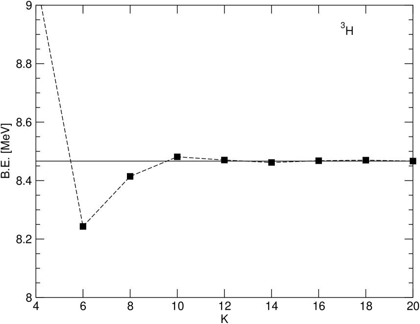
Figure 1: Triton binding energy with AV18+UrbIX (no isospin mixing) as function of grand angular momentum quantum number $K$.

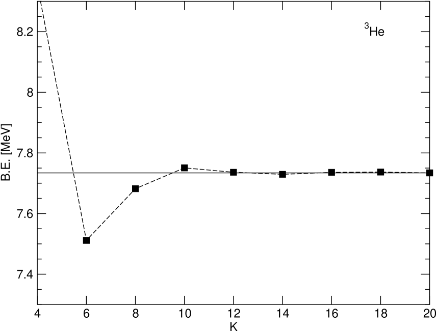
Figure 2: Same as Fig. 1 but for ³He.

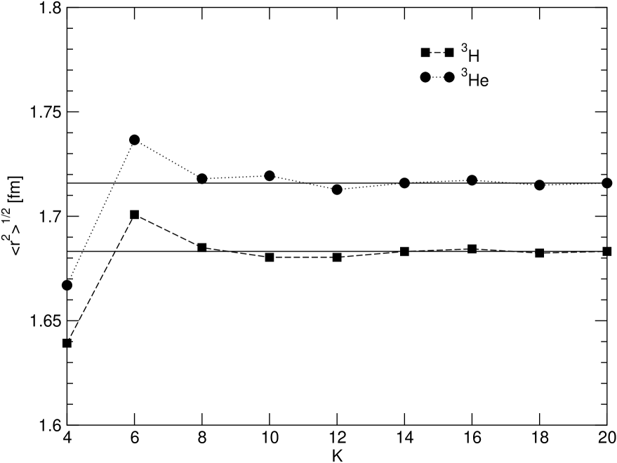
Figure 3: ³H and ³He matter radii with AV18+UrbIX (no isospin mixing) as function of grand angular momentum quantum number $K$.

In Fig. 1 we show the binding energy of the triton as function of the grand angular momentum quantum number $K$. One observes a very good convergence pattern. In fact already with $K=8$ one has only a difference of about 50 keV with the value of $K=20$. This difference is further reduced to about 20 keV with $K=10$, while with $K=12$ one has essentially the final result. In Fig. 2 we show the corresponding results for ³He. One finds a very similar picture as in Fig. 1, i.e. again an excellent convergence. In Fig. 3 we illustrate the results for the matter radii of ³H and ³He. Also in these cases a very good convergence is evident with almost identical convergence patterns for ³H and ³He.

In Table I we list our results for the triton binding energy and the probabilities for the different angular momentum components together with those of Table I in ELOT2 , where the inelastic longitudinal electron scattering form factors of the three–nucleon systems were calculated (for this comparison the electromagnetic part of AV18 is not included). There is a good agreement for the various probabilities and a small difference of about 40 keV for the binding energy.

With an inclusion of the electromagnetic interaction of AV18 we obtain the results given in Table II, which are compared to those of BoPi . The comparison of the various results reveals an excellent agreement for the various ground state properties obtained in the different calculations, e.g., the maximal difference for the binding energy is 6 keV for both three–body nuclei. Thus we may conclude that 3N forces can be included in the EIHH formalism with high precision. This is an important finding opening up the way to include 3N forces also for systems with $A>3$ in this approach.

Appendix: Multipole expansion and matrix elements of 3N forces

We consider the Urbana UrbIX and Tucson-Melbourne TM versions of 3N forces. To calculate their matrix elements (ME) we first represent the 3N force operators as expansions over irreducible space tensors. We shall list these expansions in two different forms.

The Urbana or Tucson-Melbourne 3N forces $v_{123}^{[3]}$ are given by a sum $\sum_{cyc}V_{ijk}$ taken over cyclic permutations of particles 1,2,3. Each of the three terms in the sum gives the same contribution to ME between states antisymmetric with respect to nucleon permutations. Each of the terms $V_{ijk}$ is also symmetric with respect to interchange of two of the three nucleons (in our notation they are nucleons $i$ and $j$). When Jacobi vectors are constructed in the natural order the spatial components of basis states are chosen to be symmetric or antisymmetric with respect to the interchange of nucleons 1 and 2. Then it is convenient to use the $V_{123}$ component of the force for the calculation of ME. The expression for this component is of the form carlsonetal83

$$V_{123}=\bigl{(}A_{2\pi}\{x_{13},x_{23}\}+B_{123}\{z_{13},z_{23}\}\bigr{)}\{{\vec{\tau}}_{1}\cdot{\vec{\tau}}_{3},{\vec{\tau}}_{2}\cdot{\vec{\tau}}_{3}\}$$ (A.1)

$$+C_{2\pi}[x_{13},x_{23}][{\vec{\tau}}_{1}\cdot{\vec{\tau}}_{3},{\vec{\tau}}_{2}\cdot{\vec{\tau}}_{3}]+U_{0}\left(T_{13}T_{23}\right)^{2}.$$ (A.2)

Here $[\ldots\,,\,\ldots]$ and $\{\ldots\,,\,\ldots\}$ mean commutator and anticommutator, respectively, while

$$x_{ij}={\vec{\sigma}}_{i}\cdot{\vec{\sigma}}_{j}Y_{ij}+S_{ij}T_{ij},\qquad z_{ij}={\vec{\sigma}}_{i}\cdot{\vec{\sigma}}_{j}+S_{ij},$$

where $Y_{ij}\equiv Y(r_{ij})$ and $T_{ij}\equiv T(r_{ij})$ are the regularized Yukawa and tensor functions, respectively. As customary $S_{ij}$ is the tensor operator, and $A_{2\pi}$, $C_{2\pi}$, and $U_{0}$ are the strength constants (for the Urbana models $C_{2\pi}=(1/4)A_{2\pi}$). The numerical values of $A_{2\pi}$ and $U_{0}$ that correspond to the Urbana IX model are listed in UrbIX . The quantity $B_{ijk}\equiv B(r_{ik},r_{jk})$ is different from zero only in the Tucson-Melbourne model TM .

In what follows we use the notation $\vec{\sigma}_{i}$ and $\vec{\tau}_{i}$ for nucleon spin and isospin operators. We use the following notation for tensor products of irreducible tensor operators

$$(A_{a}\otimes B_{b})_{\lambda\mu} = \sum_{\alpha+\beta=\mu}\langle a\alpha b\beta|\lambda\mu\rangle A_{a\alpha}B_{b\beta},\qquad(A_{a}\cdot B_{a})=\sum_{\alpha}A_{a\alpha}B_{a,-\alpha}(-1)^{\alpha},$$

$$(A_{a}\otimes B_{b})_{\lambda\mu}^{C} = \sum_{\alpha+\beta=\mu}\langle{a\alpha b\beta}|{\lambda\mu}\rangle[A_{a\alpha},B_{b\beta}],\qquad(A_{a}\otimes B_{b})_{\lambda\mu}^{A}=\sum_{\alpha+\beta=\mu}\langle{a\alpha b\beta}|{\lambda\mu}\rangle\{A_{a\alpha},B_{b\beta}\},$$

and also the notation for irreducible spin tensors

$$\Sigma_{ij}^{\lambda\mu}=(\vec{\sigma}_{i}\otimes\vec{\sigma}_{j})_{\lambda\mu}\,,\,\,\,\,\,\,\,\Sigma_{ij,k}^{\lambda,\Lambda M}=\left(\vec{\sigma}_{k}\otimes(\vec{\sigma}_{i}\otimes\vec{\sigma}_{j})_{\lambda}\right)_{\Lambda M}.$$ (A.3)

Use of spherical harmonics and their tensor products as irreducible space tensors gives the expansion of $V_{123}$ in the form

$$V_{123}=W_{0}+\left(Y_{2}(\hat{r}_{13})\cdot W_{2}^{TY}\right)+\left(Y_{2}(\hat{r}_{23})\cdot W_{2}^{YT}\right)+\sum_{\lambda=0}^{3}\left(Y_{\lambda}^{22}(\hat{r}_{13},\hat{r}_{23})\cdot W_{\lambda}^{TT}\right),$$ (A.4)

where $Y_{\lambda\mu}^{22}(\hat{r}_{13},\hat{r}_{23})=\left(Y_{2}(\hat{r}_{13})\otimes Y_{2}(\hat{r}_{23})\right)_{\lambda\mu}$, $\hat{r}_{ij}$ stands for the unit relative vector of nucleons $i$ and $j$ ($\vec{r}_{ij}=\vec{r}_{i}-\vec{r}_{j}$). The quantities $W_{0}$, $W_{2\mu}^{TY}$, $W_{2\mu}^{YT}$ and $W_{\lambda\mu}^{TT}$ are irreducible tensors with respect to spin variables of the ranks 0, 2, and $\lambda$, respectively. One has

$$W_{0} = U_{0}(T_{13}T_{23})^{2}+(A_{2\pi}Y_{13}Y_{23}+B_{123})\{{\vec{\tau}}_{1}\cdot{\vec{\tau}}_{3},{\vec{\tau}}_{2}\cdot{\vec{\tau}}_{3}\}\{{\vec{\sigma}}_{1}\cdot{\vec{\sigma}}_{3},{\vec{\sigma}}_{2}\cdot{\vec{\sigma}}_{3}\}$$

$$+C_{2\pi}Y_{13}Y_{23}[{\vec{\tau}}_{1}\cdot{\vec{\tau}}_{3},{\vec{\tau}}_{2}\cdot{\vec{\tau}}_{3}][{\vec{\sigma}}_{1}\cdot{\vec{\sigma}}_{3},{\vec{\sigma}}_{2}\cdot{\vec{\sigma}}_{3}],$$

$$W_{2\mu}^{TY} = \sqrt{\frac{24\pi}{5}}\left[(A_{2\pi}T_{13}Y_{23}+B_{123})\{{\vec{\tau}}_{1}\cdot{\vec{\tau}}_{3},{\vec{\tau}}_{2}\cdot{\vec{\tau}}_{3}\}\{\Sigma^{2\mu}_{13},{\vec{\sigma}}_{2}\cdot{\vec{\sigma}}_{3}\}\right.$$

$$+\left.C_{2\pi}T_{13}Y_{23}[{\vec{\tau}}_{1}\cdot{\vec{\tau}}_{3},{\vec{\tau}}_{2}\cdot{\vec{\tau}}_{3}][\Sigma^{2\mu}_{13},{\vec{\sigma}}_{2}\cdot{\vec{\sigma}}_{3}]\right],$$

$$W_{\lambda\mu}^{TT} = \frac{24\pi}{5}(-1)^{\lambda}\left[(A_{2\pi}T_{13}T_{23}+B_{123})\{{\vec{\tau}}_{1}\cdot{\vec{\tau}}_{3},{\vec{\tau}}_{2}\cdot{\vec{\tau}}_{3}\}(\Sigma^{2}_{13}\otimes\Sigma^{2}_{23})_{\lambda\mu}^{A}\right.$$ (A.5)

$$\left.+C_{2\pi}T_{13}T_{23}[{\vec{\tau}}_{1}\cdot{\vec{\tau}}_{3},{\vec{\tau}}_{2}\cdot{\vec{\tau}}_{3}](\Sigma^{2}_{13}\otimes\Sigma^{2}_{23})_{\lambda\mu}^{C}\right],$$

and $W_{2\mu}^{YT}$ = (${\hat{12}})W_{2\mu}^{TY}$. The formulae above are obtained using the following expression for the tensor operator

$$S_{ij}\equiv 3({\vec{\sigma}}_{i}\cdot{\hat{r}}_{ij})({\vec{\sigma}}_{j}\cdot{\hat{r}}_{ij})-({\vec{\sigma}}_{i}\cdot{\vec{\sigma}}_{j})=\sqrt{\frac{24\pi}{5}}(Y_{2}({\hat{r}}_{ij})\cdot\Sigma^{2}_{ij})$$

and the recoupling

$$(Y_{2}({\hat{r}}_{13})\cdot\Sigma^{2}_{13})(Y_{2}({\hat{r}}_{23})\cdot\Sigma^{2}_{23})=\sum_{\lambda=0}^{3}(-1)^{\lambda}\bigl{(}Y_{\lambda}^{22}({\hat{r}}_{13},{\hat{r}}_{23})\cdot(\Sigma^{2}_{13}\otimes\Sigma^{2}_{23})_{\lambda}\bigl{)}$$

(for $\lambda=4$ the quantity $(\Sigma^{2}_{13}\otimes\Sigma^{2}_{23})_{\lambda\mu}$ vanishes).

The ME of the scalar products entering (A.4) are expressed in the standard way in terms of spatial reduced ME and spin–isospin ME reduced with respect to spin. The latter ME may be calculated directly writing down all the quantities depending on spin and isospin in terms of $\sigma_{i;0,\pm}$ and $\tau_{i;0,\pm}$. One may also employ the expansions over the tensors of Eq. (A.3) form with subsequent use of the ME (A.40), (A.48). To obtain these expansions we perform recouplings, make use of the values of $\{\sigma_{3\mu},\sigma_{3\nu}\}$ and $[\sigma_{3\mu},\sigma_{3\nu}]$ Varshalovich and also perform simple summations of Clebsch–Gordan coefficients Varshalovich . As a result we get the following expression for the 3N force

$$V_{123} = 4\sqrt{3}(\vec{\tau}_{1}\otimes\vec{\tau}_{2})_{0}\Big{\{}(A_{2\pi}Y_{13}Y_{23}+B_{123})\sqrt{3}\Sigma_{12}^{0}$$ (A.18)

$$\hskip 59.75095pt-\sqrt{\frac{24\pi}{5}}\left(1+(\hat{12})\right)(A_{2\pi}T_{13}Y_{23}+B_{123})(Y_{2}(\hat{r}_{13})\cdot\Sigma_{12}^{2})$$

$$+5\frac{24\pi}{5}(A_{2\pi}T_{13}T_{23}+B_{123})\sum_{\lambda=0}^{3}\sqrt{3(2\lambda+1)}\left\{\begin{array}[]{ccc}1&1&2\\ 1&1&2\\ \lambda&0&\lambda\end{array}\right\}(Y_{\lambda}^{22}(\hat{r}_{13},\hat{r}_{23})\cdot\Sigma_{12}^{\lambda})\Big{\}}$$

$$+4\sqrt{3}C_{2\pi}\left(\vec{\tau}_{3}\otimes(\vec{\tau}_{1}\otimes\vec{\tau}_{2})_{1}\right)_{0}\Big{\{}2\sqrt{3}Y_{13}Y_{23}\Sigma_{12,3}^{1,0}$$

$$\hskip 59.75095pt+\left(1+(\hat{12})\right)T_{13}Y_{23}\left(Y_{2}(\hat{r}_{13})\cdot(\Sigma_{12,3}^{1,2}+\sqrt{3}\Sigma_{12,3}^{2,2})\right)$$

$$-10\sqrt{3}T_{13}T_{23}\sum_{\Lambda=0}^{3}\Bigl{(}Y_{\Lambda}^{22}(\hat{r}_{13},\hat{r}_{23})\cdot\sum_{\lambda}(-1)^{\lambda+\Lambda}\sqrt{2\lambda+1}\left\{\begin{array}[]{ccc}1&1&2\\ 1&1&2\\ \lambda&1&\Lambda\end{array}\right\}\Sigma^{\lambda,\Lambda}_{12,3}\Bigl{)}\Big{\}}$$

$$+U_{0}(T_{12}T_{13})^{2}.$$

Another multipole expansion of the force is obtained when the quantities

$$X_{ij}^{\lambda\mu}=(\hat{r}_{1i}\otimes\hat{r}_{1j})_{\lambda\mu}\,,\,\,\,\,\,\,X_{ij,kl}^{(\lambda,\lambda^{\prime})\Lambda M}=\left((\hat{r}_{1i}\otimes\hat{r}_{1j})_{\lambda}\otimes(\hat{r}_{1k}\otimes\hat{r}_{1l})_{\lambda^{\prime}}\right)_{\Lambda M}\,.$$ (A.19)

are used as spatial tensors and, moreover, an expansion of spin–isospin operators over the tensors of Eq. (A.3) form is performed. In this case we assume use of Jacobi vectors constructed in the reversed order and for the calculation of ME we employ the component $V_{231}$ of the force. We rewrite it in the following form:

$$V_{231} = A_{2\pi}(2{\vec{\tau}}_{2}\cdot{\vec{\tau}}_{3})\big{(}F_{TT}(\vec{\sigma}_{2}\cdot\hat{r}_{12})(\vec{\sigma}_{3}\cdot\hat{r}_{13})(\hat{r}_{12}\cdot\hat{r}_{13})+F_{YY}({\vec{\sigma}}_{2}\cdot{\vec{\sigma}}_{3})$$ (A.23)

$$\hskip 28.45274pt+F_{TY}(\vec{\sigma}_{2}\cdot\hat{r}_{12})(\vec{\sigma}_{3}\cdot\hat{r}_{12})+F_{YT}(\vec{\sigma}_{2}\cdot\hat{r}_{13})(\vec{\sigma}_{3}\cdot\hat{r}_{13})\big{)}$$

$$-C_{2\pi}(2\vec{\tau}_{1}\cdot\vec{\tau}_{2}\times\vec{\tau}_{3})\big{(}F_{TT}(\vec{\sigma}_{2}\cdot\hat{r}_{12})(\vec{\sigma}_{3}\cdot\hat{r}_{13})(\vec{\sigma}_{1}\cdot\hat{r}_{12}\times\hat{r}_{13})+F_{YY}(\vec{\sigma}_{1}\cdot\vec{\sigma}_{2}\times\vec{\sigma}_{3})$$

$$\hskip 28.45274pt+F_{TY}(\vec{\sigma}_{2}\cdot\hat{r}_{12})(\vec{\sigma}_{3}\cdot\vec{\sigma}_{1}\times\hat{r}_{12})+F_{YT}(\vec{\sigma}_{3}\cdot\hat{r}_{13})(\vec{\sigma}_{1}\cdot\vec{\sigma}_{2}\times\hat{r}_{13})\big{)}$$

$$+ B_{231}(2{\vec{\tau}}_{2}\cdot{\vec{\tau}}_{3})18(\vec{\sigma}_{2}\cdot\hat{r}_{12})(\vec{\sigma}_{3}\cdot\hat{r}_{13})(\hat{r}_{12}\cdot\hat{r}_{13})+U_{0}(T_{12}T_{13})^{2}$$ (A.24)

with $F_{TT}=18T_{12}T_{13}$ and

$$F_{YY}=2(Y_{12}-T_{12})(Y_{13}-T_{13})\,,\,\,\,F_{TY}=6T_{12}(Y_{13}-T_{13})\,,\,\,\,F_{YT}=6(Y_{12}-T_{12})T_{13}\,.$$ (A.25)

After a recoupling of the various operators one obtains

$$V_{231} = -2\sqrt{3}A_{2\pi}(\vec{\tau}_{2}\otimes\vec{\tau}_{3})_{0}\Big{\{}\Sigma_{23}^{0}\cdot[-\sqrt{3}(F_{TT}+18\frac{B_{231}}{A_{2\pi}})X_{23}^{0}X_{23}^{0}-\frac{1}{\sqrt{3}}(3F_{YY}+F_{TY}+F_{YT})]$$ (A.39)

$$\hskip 88.2037pt+\Sigma_{23}^{1}\cdot[\sqrt{3}(F_{TT}+18\frac{B_{231}}{A_{2\pi}})X_{23}^{0}X_{23}^{1}]$$

$$\hskip 88.2037pt+\Sigma_{23}^{2}\cdot[-\sqrt{3}(F_{TT}+18\frac{B_{231}}{A_{2\pi}})X_{23}^{0}X_{23}^{2}+(F_{TY}X_{22}^{2}+F_{YT}X_{33}^{2})]\Big{\}}$$

$$-4\sqrt{3}C_{2\pi}\left(\vec{\tau}_{1}\otimes(\vec{\tau}_{2}\otimes\vec{\tau}_{3})_{1}\right)_{0}\Big{\{}\Sigma_{23,1}^{1,0}\cdot\sqrt{3}[\left\{\begin{array}[]{ccc}1&1&1\\ 1&0&1\end{array}\right\}(F_{TY}+F_{YT})-F_{YY}-\frac{F_{TT}}{\sqrt{3}}X_{23,23}^{(1,1)0}]$$

$$\hskip 122.34692pt+\Sigma_{23,1}^{0,1}\cdot[F_{TT}X_{23,23}^{(1,0)1}]+\Sigma_{23,1}^{2,1}\cdot[F_{TT}X_{23,23}^{(1,2)1}]$$

$$\hskip 122.34692pt+\Sigma_{23,1}^{1,2}\cdot[-3\left\{\begin{array}[]{ccc}1&1&1\\ 1&2&1\end{array}\right\}(F_{TY}X_{22}^{2}+F_{YT}X_{33}^{2})-F_{TT}X_{23,23}^{(1,1)2}]$$

$$\hskip 122.34692pt+\Sigma_{23,1}^{2,2}\cdot[\sqrt{15}\left\{\begin{array}[]{ccc}1&1&2\\ 1&2&1\end{array}\right\}(F_{TY}X_{22}^{2}-F_{YT}X_{33}^{2})-F_{TT}X_{23,23}^{(1,2)2}]$$

$$\hskip 122.34692pt+\Sigma_{23,1}^{2,3}\cdot[F_{TT}X_{23,23}^{(1,2)3}]\Big{\}}+U_{0}(T_{12}T_{13})^{2}.$$

For the spin operators of Eq. (A.3) one finds the following reduced matrix elements

$$\langle(s_{1};(s_{2};s_{3})S_{23})S_{123}||(\vec{\sigma}_{2}\otimes\vec{\sigma}_{3})_{\lambda}||(s_{1};(s_{2};s_{3})S^{\prime}_{23})S^{\prime}_{123}\rangle$$ (A.40)

$$= 6(-)^{1/2+\lambda+S^{\prime}_{23}+S_{123}}\sqrt{(2S_{123}+1)(2S^{\prime}_{123}+1)}\left\{\begin{array}[]{ccc}S_{23}&S_{123}&\frac{1}{2}\\ S^{\prime}_{123}&S^{\prime}_{23}&\lambda\end{array}\right\}$$ (A.47)

$$\times\sqrt{(2S_{23}+1)(2S^{\prime}_{23}+1)(2\lambda+1)}\left\{\begin{array}[]{ccc}\frac{1}{2}&\frac{1}{2}&S_{23}\\ \frac{1}{2}&\frac{1}{2}&S^{\prime}_{23}\\ 1&1&\lambda\end{array}\right\}\,,$$

$$\langle(s_{1};(s_{2};s_{3})S_{23})S_{123}||(\vec{\sigma}_{1}\otimes(\vec{\sigma}_{2}\otimes\vec{\sigma}_{3})_{\lambda})_{\Lambda}||(s_{1};(s_{2};s_{3})S^{\prime}_{23})S^{\prime}_{123}\rangle$$ (A.48)

$$= 6^{\frac{3}{2}}\sqrt{(2S_{123}+1)(2S^{\prime}_{123}+1)(2\Lambda+1)}\left\{\begin{array}[]{ccc}\frac{1}{2}&S_{23}&S_{123}\\ \frac{1}{2}&S^{\prime}_{23}&S^{\prime}_{123}\\ 1&\lambda&\Lambda\end{array}\right\}$$ (A.56)

$$\times\sqrt{(2S_{23}+1)(2S^{\prime}_{23}+1)(2\lambda+1)}\left\{\begin{array}[]{ccc}\frac{1}{2}&\frac{1}{2}&S_{23}\\ \frac{1}{2}&\frac{1}{2}&S^{\prime}_{23}\\ 1&1&\lambda\end{array}\right\}\,.$$

The isospin operators of Eqs. (A.39) and (A.18) lead to corresponding expressions for the reduced matrix elements.

For the calculation of the spatial matrix elements one has to perform a six–dimensional integration. For this integration we use the same technique as first used in ELOT and explicitly described in Efros . For the Jacobi vectors (see section III)

$${\vec{\eta}}_{A-1}=\rho^{[3]}_{int}\,\sin\theta^{[3]}_{int}\,{\hat{\eta}}_{A-1}\,,\,\,\,\,\,\,\,\,\,\,\,{\vec{\eta}}_{A-2}=\rho^{[3]}_{int}\,\cos\theta^{[3]}_{int}\,{\hat{\eta}}_{A-2}$$ (A.57)

one chooses a special reference frame in which ${\hat{\eta}}_{A-1}$ turns into a vector ${\hat{\zeta}}_{A-1}=\hat{z}$ and ${\hat{\eta}}_{A-2}$ turns into a vector ${\hat{\zeta}}_{A-2}$ that lies in the ($x$-$z$) plane. Then one replaces the angles $\theta^{[3]}_{int}$, ${\hat{\eta}}_{A-1}$, and ${\hat{\eta}}_{A-2}$ by

$$x=cos(2\theta^{[3]}_{int})\,,\hskip 56.9055pty={\hat{\eta}}_{A-1}\cdot{\hat{\eta}}_{A-2}\,,$$ (A.58)

and the three Euler angles $\omega$. This leads to the following volume element

$$d{\vec{\eta}}_{A-1}d{\vec{\eta}}_{A-2}=(\rho^{[3]}_{int})^{5}d\rho^{[3]}_{int}\frac{1}{8}\sqrt{1-x^{2}}dxd{\hat{\eta}}_{A-1}d{\hat{\eta}}_{A-2}=(\rho^{[3]}_{int})^{5}d\rho^{[3]}_{int}\frac{1}{8}\sqrt{1-x^{2}}dxdyd\omega\,.$$ (A.59)

With this parametrization one obtains for the three–body HH functions

$$Y_{KLM}^{\ell_{1}\ell_{2}}(\Omega) = \psi_{K}^{\ell_{1}\ell_{2}}(x)[Y_{\ell_{1}m_{1}}({\hat{\eta}}_{A-1})\otimes Y_{\ell_{2}m_{2}}({\hat{\eta}}_{A-2})]_{LM}$$ (A.60)

$$= \psi_{K}^{\ell_{1}\ell_{2}}(x)\sum_{M^{\prime}}D^{(L)}_{M^{\prime}M}(\omega)[Y_{\ell_{1}m_{1}}({\hat{\zeta}}_{A-1})\otimes Y_{\ell_{2}m_{2}}({\hat{\zeta}}_{A-2}]_{LM^{\prime}}$$ (A.61)

$$= \sum_{M^{\prime}}D^{(L)}_{M^{\prime}M}(\omega)Y_{KLM^{\prime}}^{\ell_{1}\ell_{2}}(x,y)\,.$$ (A.62)

The five–dimensional integration in $dxdyd\omega$ can be reduced to a two–dimensional one. In fact after some algebra one finds for a coordinate space operator $V_{\lambda\mu}(\rho^{[3]}_{int},\Omega^{[3]}_{int})$ of rank $\lambda$ and projection $\mu$ the following reduced matrix element

$$\langle KL\ell_{1}\ell_{2}||V_{\lambda}(\rho^{[3]}_{int},\Omega^{[3]}_{int})||K^{\prime}L^{\prime}\ell^{\prime}_{1}\ell^{\prime}_{2}\rangle = \sum_{MM^{\prime}\mu}(-)^{L+M}\left(\begin{array}[]{ccc}L&\lambda&L^{\prime}\\ -M&\mu&M^{\prime}\end{array}\right)$$ (A.66)

$$\times\pi^{2}\int dx\sqrt{1-x^{2}}dyY_{KLM}^{\;\ell_{1}\ell_{2}*}(x,y)V_{\lambda\mu}(\rho^{[3]}_{int},x,y)Y_{K^{\prime}L^{\prime}M^{\prime}}^{\ell^{\prime}_{1}\ell^{\prime}_{2}}(x,y)\,.$$

Acknowledgments

The work of N.B. was supported by the ISRAEL SCIENCE FOUNDATION (grant no. 202/02), V.D.E. acknowledges the support of the Russian Ministry of Industry and Science, grant NS–1885.2003.2.

Table 1: ³H ground state properties with AV18+UrbIX (no electromagnetic interaction, no isospin mixing) for binding energy BE and probabilities of total orbital angular momentum components in %

	this work	CHH ELOT2
BE [MeV]	8.508	8.47
S-wave	89.504	89.55
S′-wave	1.061	1.05
P-wave	0.135	0.13
D-wave	9.300	9.27

Table 2: Same as Table I but with inclusion of electromagnetic interaction (no isospin mixing)

	this work	Bochum BoPi	Pisa BoPi
BE [MeV]	8.468	8.470	8.474
S-wave	89.516	89.512	89.509
S′-wave	1.059	1.051	1.055
P-wave	0.135	0.135	0.135
D-wave	9.291	9.302	9.301

Table 3: Same as Table II but for ³He

	this work	Bochum BoPi	Pisa BoPi
BE [MeV]	7.736	7.738	7.742
S-wave	89.385	89.391	89.378
S′-wave	1.246	1.229	1.242
P-wave	0.132	0.132	0.131
D-wave	9.238	9.248	9.249

References

• (1) Steven C. Pieper and R.B. Wiringa, Ann. Rev. Nucl. Part. Sci. 51 (2001) 53.
• (2) V.D. Efros, W. Leidemann, G. Orlandini and E.L. Tomusiak, Phys. Lett. B484, 223 (2000).
• (3) V.D. Efros, W. Leidemann, G. Orlandini and E.L. Tomusiak, Phys. Rev. C69, 044001 (2004).
• (4) A. Nogga, A. Kievsky, H. Kamada, W. Glöckle, L.E. Marcucci, S. Rosati and M. Viviani, Phys. Rev. C 67, 034004 (2003).
• (5) A. Nogga, H. Kamada, W. Glöckle and B.R. Barrett, Phys. Rev. C65, 054003 (2002).
• (6) D.C.J. Marsden, P. Navrátil, S.A. Coon and B.R. Barrett, Phys. Rev. C66, 044007 (2002); P. Navrátil and W.E. Ormand, $ibid$ C68, 034305 (2003).
• (7) N. Barnea, W. Leidemann and G. Orlandini, Phys. Rev. C61, 054001 (2000).
• (8) R.B. Wiringa, V.G.J. Stoks and R. Schiavilla, Phys. Rev. C51, 38 (1995).
• (9) B.S. Pudliner, V.R. Pandharipande, J. Carlson, S.C. Pieper and R.B. Wiringa, Phys. Rev. C56, 1720 (1997).
• (10) K. Suzuki and S.Y. Lee, Prog. Theor. Phys. 64, 2091 (1980); K. Suzuki, $ibid$ 68, 246 (1982); K. Suzuki and R. Okamoto, $ibid$ 70, 439 (1983).
• (11) N. Barnea, W. Leidemann and G. Orlandini, Nucl. Phys. A693, 565 (2001).
• (12) N. Barnea, W. Leidemann and G. Orlandini, Phys. Rev. C67, 054003 (2003).
• (13) S.A. Coon, M.D. Scadron, P.C. McNamee, B.R. Barrett, D.W.E. Blatt and B.H.J. McKellar, Nucl. Phys. A317, 242 (1979); S.A. Coon and W. Glöckle, Phys. Rev. C23, 1790 (1981).
• (14) J. Carlson, V.R. Pandharipande and R.B. Wiringa, Nucl. Phys., A401, 59 (1983).
• (15) D.A. Varshalovich, A.N. Moskalev and V.K. Khersonskii, Quantum Theory of Angular Momentum, World Scientific, Singapore, 1988.
• (16) V.D. Efros, Few-Body Syst. 32, 169 (2002).