Parity-Violating Interaction Effects in the System
Abstract
We investigate parity-violating observables in the system, including the longitudinal asymmetry and neutron-spin rotation in elastic scattering, the photon asymmetry in radiative capture, and the asymmetries in deuteron photo-disintegration in the threshold region and electro-disintegration in quasi-elastic kinematics. To have an estimate of the model dependence for the various predictions, a number of different, latest-generation strong-interaction potentials—Argonne , Bonn 2000, and Nijmegen I—are used in combination with a weak-interaction potential consisting of -, -, and -meson exchanges—the model known as DDH. The complete bound and scattering problems in the presence of parity-conserving, including electromagnetic, and parity-violating potentials is solved in both configuration and momentum space. The issue of electromagnetic current conservation is examined carefully. We find large cancellations between the asymmetries induced by the parity-violating interactions and those arising from the associated pion-exchange currents. In the capture, the model dependence is nevertheless quite small, because of constraints arising through the Siegert evaluation of the relevant matrix elements. In quasi-elastic electron scattering these processes are found to be insignificant compared to the asymmetry produced by - interference on individual nucleons. These two experiments, then, provide clean probes of different aspects of weak-interaction physics associated with parity violation in the system. Finally, we find that the neutron spin rotation in elastic scattering and asymmetry in deuteron disintegration by circularly-polarized photons exhibit significant sensitivity both to the values used for the weak vector-meson couplings in the DDH model and to the input strong-interaction potential adopted in the calculation. This reinforces the conclusion that these short-ranged meson couplings are not in themselves physical observables, rather the parity-violating mixings are the physically relevant parameters.
pacs:
21.30.+y, 24.80.-x, 25.40.CmI Introduction
A new generation of experiments have recently been completed, or are presently under way or in their planning phase to study the effects of parity-violating (PV) interactions in elastic scattering [1], radiative capture [2] and deuteron electro-disintegration [3] at low energies. There is also considerable interest in determining the extent to which hadronic weak interactions can affect the longitudinal asymmetry measured by the SAMPLE collaboration in quasi-elastic scattering of polarized electrons off the deuteron [4], and therefore influence the extraction from these data (and those on the proton [5]) of the nucleon’s strange magnetic and axial-vector form factors at four-momentum transfers squared of and (GeV/c)2.
The present is the third in a series of papers dealing with the theoretical investigation of PV interaction effects in two-nucleon systems. The first [6] was devoted to elastic scattering, and presented a calculation of the longitudinal asymmetry induced by PV interactions in the lab-energy range 0–350 MeV. The second [7] provided a rather cursory account of a study of the PV asymmetries in radiative capture at thermal neutron energies and in deuteron electro-disintegration at quasi-elastic kinematics. This work further extends that of Ref. [7] by investigating the neutron spin rotation at zero energy and the longitudinal asymmetry in elastic scattering at lab energies between 0 and 350 MeV, and the photon-helicity dependence of the cross-section from threshold up to energies of 20 MeV. It also provides a thorough analysis of the results already presented in Ref. [7].
We adopt the PV potential developed by Desplanques et al. [8] over twenty years ago, the so-called DDH model. In the sector, it is conveniently parameterized in terms of -, -, and -meson exchanges. In Ref. [8] the pion and vector-meson weak coupling constants were estimated within a quark model approach incorporating symmetry techniques like SU(6)W and current algebra requirements. Due to limitations inherent to such an analysis, however, the coupling constants so determined had rather wide ranges of allowed values.
Our prime motivations are to develop a systematic and consistent framework for studying PV observables in the few-nucleon systems, where accurate microscopic calculations are feasible, and to use available and forthcoming experimental data on these observables to constrain the strengths of the short- and long-range parts of the two-nucleon weak interaction. Indeed, in Ref. [6] we showed, for the case of the longitudinal asymmetry measured in elastic scattering, how available experimental data provide strong constraints on allowable combinations of - and -meson weak coupling constants.
The remainder of the present paper is organized as follows. In Sec. II the PV potential as well as the parity-conserving strong-interaction potentials used in this work are briefly discussed, while in Sec. III the model for the nuclear electro-weak currents is described, including the electromagnetic two-body terms induced by the presence of PV interactions. In Sec. IV a self-consistent treatment of the bound- and scattering-state problems in both configuration and momentum spaces is provided, patterned after that of Ref. [6], and in Sec. V explicit expressions are derived for the longitudinal asymmetry and spin rotation in elastic scattering, the photon asymmetry in radiative capture, and the asymmetries in deuteron photo- and electro-disintegration. In Sec. VI the techniques used to calculate the PV observables are briefly reviewed, while in Sec. VII a fairly detailed analysis of the results is offered. Finally, Sec. VIII contains some concluding remarks.
II Parity-Conserving and Parity-Violating Potentials
The parity-conserving (PC), strong-interaction potentials used in the present work are the Argonne (AV18) [9], Nijmegen I (NIJM-I) [10], and CD-Bonn (BONN) [11] models. They were discussed in Ref. [6] in connection with the calculation of the longitudinal asymmetry in elastic scattering. Here, we briefly summarize a few salient points.
The AV18 and NIJM-I potentials were fitted to the Nijmegen database of 1992 [12, 13], consisting of 1787 and 2514 scattering data, and both produced per datum close to one. The latest version of the charge-dependent Bonn potential, however, has been fit to the 1999 database, consisting of 2932 and 3058 data, for which it gives per datum of 1.01 and 1.02, respectively [11]. The substantial increase in the number of data is due to the development of novel experimental techniques—internally polarized gas targets and stored, cooled beams. Indeed, using this technology, IUCF has produced a large number of spin-correlation parameters of very high precision, see for example Ref. [14]. It is worth noting that the AV18 potential, as an example, fits the post-1992 and both pre- and post-1992 () data with ’s of 1.74 (1.02) and 1.35 (1.07), respectively [11]. Therefore, while the quality of their fits (to the data) has deteriorated somewhat in regard to the extended 1999-database, the AV18 and NIJM-I models can still be considered “realistic”.
As already mentioned in Sec. I, the form of the parity-violating (PV) weak-interaction potential was derived in Ref. [8]—the DDH model. In the isospin space of the pair it is expressed as
| (1) |
where =0 or 1. The diagonal and off-diagonal terms are then obtained as
| (2) | |||||
| (3) |
| (4) | |||||
| (5) |
and =. In the equations above the relative position and momentum are defined as and , respectively, denotes the anticommutator, and , , , and are the proton, pion, -meson, -meson masses, respectively. The Yukawa function , suitably modified by the inclusion of monopole form factors, is given by
| (6) |
where . Note that denotes , and that the terms proportional to in Eqs. (3) and (5) are usually written in the form of a commutator, since
| (7) |
Finally, the values for the strong-interaction -meson pseudoscalar coupling constant , and - and -meson vector and tensor coupling constants and , as well as for the cutoff parameters , are taken from the BONN model [11], and are listed in Table I. The weak-interaction vector-meson coupling constants and correspond to the following combinations of DDH parameters
| (8) | |||||
| (9) |
where =0,1. The values for these and for , , and are listed in Table I. Note that we have taken the linear combination of - and -meson weak coupling constants corresponding to elastic scattering from the earlier analysis [6] of these experiments. The remaining couplings are the “best value” estimates, suggested in Ref. [8].
III Electromagnetic and Neutral Weak Current Operators
The electromagnetic current and charge operators, respectively and , are expanded into a sum of one- and two-body terms
| (10) |
and similarly for . The one-body terms have the standard expressions obtained from a non-relativistic reduction of the covariant single-nucleon current [15]. The two-body charge operators are those derived in Ref. [16]; they only enter in the calculation of the asymmetry in the deuteron electro-disintegration at quasi-elastic kinematics, and will not be discussed further here.
The two-body currents have terms associated with the parity-conserving (PC) and parity-violating (PV) components of the interaction, respectively and . The operators were derived explicitly in Ref. [17], and a complete listing of those relative to the Argonne (AV18) interaction [9] has been given most recently in Ref. [15]. Only the two-body currents associated with - and -exchange are retained in the case of the Bonn (BONN) [11] and Nijmegen-I (NIJM-I) [10] interactions.
In addition to these, the purely transverse two-body currents associated with the excitation of -isobars and the and mechanisms are included in all calculations. Again explicit expressions for these operators can be found in Ref. [15]. Note, however, that the -isobar degrees of freedom are treated in perturbation theory rather than with the transition-correlation-operator method [18], and that only effects due to single excitation are considered, according to Eqs. (2.15) and (3.4) in Ref. [15].
Before moving on to a discussion of the PV currents, we briefly review, for later reference, the question of conservation of the electromagnetic current for the case of the AV18. As pointed out in Ref. [15], the currents from its part (specifically, its isospin-dependent central, spin-spin, and tensor components) are strictly conserved. In a one-boson-exchange model, which the AV18 is not, these interaction components arise from - and -exchange.
The currents from the AV18 momentum-dependent (-dependent) components—the spin-orbit, , and quadratic-spin-orbit terms—are also included. In Ref. [19] and later papers, the currents from the spin-orbit term were derived by generalizing the procedure used to obtain the currents. It was assumed that the isospin-independent (isospin-dependent) central and spin-orbit interactions were due to and exchanges ( exchange), and the associated two-body currents were constructed by considering corresponding -pair diagrams involving these meson exchanges. The currents from the and quadratic-spin-orbit interactions were obtained, instead, by minimal substitution [15, 17].
The currents from the -dependent interactions are strictly not conserved, as one can easily surmise by considering their commutator with the charge density operator. For example, in the case of the isospin-dependent and interactions, this commutator requires the presence of currents with the isospin structure , which cannot be generated by minimal substitution [17].
We will return to this issue in Sec. VII B. Here, we only want to emphasize that the currents from the -dependent terms in the AV18 are short-ranged. Their contributions to isovector observables, such as, for example, the magnetic form factors of the trinucleons [20], are found to be numerically much smaller than those due to the leading currents. These currents also lead to small, although non-negligible, corrections to isoscalar observables, such as the deuteron magnetic moment and structure function [21]. However, in the case of the PV asymmetry in the radiative capture at thermal energies under consideration in the present study, they will turn out to play an important role (see Sec. VII B).
A Parity-violating currents
The DDH PV interaction [8] is parameterized in terms of -, -, and -meson exchanges. The meson-nucleon phenomenological Lagrangian densities have been given most recently in Ref. [22]. We adopt here the notation and conventions of that work, except that we use pseudo-vector coupling for the interaction Lagrangian, i.e.
| (11) |
with =. The resulting coupling is given by
| (12) |
and the current is then obtained from the Feynman amplitude in Fig. 2, panel (a). The complete PV -exchange current is derived from a non-relativistic reduction of both amplitudes in Fig. 2, and to leading order reads:
| (13) | |||||
| (14) |
where is defined as
| (15) |
= is the fractional momentum delivered to nucleon (with these definitions =), and is a short-range cutoff. In the limit of point-like couplings, the current above is identical to that listed in Eqs. (A7a) and (A9a) of Ref. [22]. -pair terms arising from the photon coupling to the nucleon line containing a PV vertex do not contribute to leading order. Lastly, we note that satisfies current conservation with the PV -exchange interaction, given in momentum space by
| (16) |
since
| (17) | |||||
| (18) |
which is easily seen to be the same as . Here denotes the isospin projection operator
| (19) |
In the present work, the PV currents induced by - and -meson exchanges have been neglected, since, due their short-range character, the associated contributions are expected to be tiny. We note, however, that in Eq. (A5) of Ref. [22] a contact term, originating from gauging the tensor coupling, has been ignored. It is given by
| (20) |
and leads, in leading order, to an additional term in Eq. (A7c) of Ref. [22] of the form
| (21) |
with defined similarly as in Eq. (15). The term above, when combined with that having the same structure in the second line of Eq. (A7c), generates a contribution proportional to which, in view of the large value of the tensor coupling constant (=6.6), is expected to be dominant in the PV -exchange current.
Finally, there is a PV one-body current originating from the nucleon’s anapole moment. It can be derived, for example, by considering pion-loop diagrams where one of the vertices involves a PV coupling; it has the structure, to leading order, given by
| (22) |
where is the four-momentum transfer, =, and the isoscalar and isovector anapole form factors are normalized as
| (23) |
with =1.6 and =0.4 from a calculation of pion-loop contributions [23]. More recent estimates of the nucleon anapole form factors predict [24, 25, 26] somewhat different values for . A complete treatment would require estimates of short-distance contributions [27] and electroweak radiative corrections. Thus, in view of the uncertainties in the quantitative estimate of these effects, we will continue to use the values above in the present study (see also Sec. VII D). Note that vanishes for real-photon transitions.
B Neutral weak currents
In the Standard Model the vector part of the neutral weak current, , is related to the isoscalar () and isovector () components of the electromagnetic current, denoted respectively as and , via
| (24) |
where is the Weinberg angle, and therefore the associated one- and two-body weak charge and current operators are easily obtained from those given in Sec III. The axial charge and current operators too have one- and two-body terms. Only the axial current
| (25) |
is needed in the present work. The one- and two-body operators are essentially those listed in Ref. [28], except for obvious changes in the isospin structure having to do with the fact that we are dealing here with neutral rather than charge-raising/lowering weak currents, and for the inclusion of nucleon and axial form factors—the parameterization adopted for these is given in Ref. [29]. Note that in Ref. [31] the relativistic corrections in and two-body axial currents were neglected, in line with the expectation, confirmed in the present study, that the associated contributions were small.
Finally, the neutral weak currents given above are at tree-level, electro-weak radiative corrections as well as strange-quark contributions to the vector and axial-vector currents [30] have been ignored. These effects have been taken into account in recent calculations of the longitudinal asymmetry in at quasi-elastic kinematics [32], however, they will not be discussed further here.
IV Formalism
In this section we discuss the scattering- and bound-state problems in the presence of a potential given by
| (26) |
where and denote the parity-conserving (PC) and parity-violating (PV) components induced by the strong (including electromagnetic) and weak interactions, respectively. The formalism and notation are similar to those developed in Ref. [6].
A Partial-wave expansions of scattering state, - and -matrices
The Lippmann-Schwinger equation for the scattering state , where is the relative momentum, , , , and =0 specify the pair spin, spin-projection, isospin, and isospin-projection states (note that the label =0 is unnecessary, since is diagonal in ), can be written as [33]
| (27) |
where is the free Hamiltonian, and are the eigenstates of , namely plane waves,
| (28) | |||||
| (29) | |||||
| (30) |
Here denotes the regular spherical Bessel function, and the following definitions have been introduced:
| (31) |
| (32) |
The factor ensures that the plane waves are properly antisymmetrized.
The -matrix corresponding to the potential is defined as [33]
| (33) |
Insertion of the plane-wave states into the right-hand-side of the Lippmann-Schwinger equation leads to
| (34) | |||||
| (35) |
from which the partial wave expansion of the scattering state is easily obtained by first noting that the potential, and hence the -matrix, can be expanded as
| (37) | |||||
with
| (38) |
After insertion of the corresponding expansion for the -matrix into Eq. (35) and a number of standard manipulations, the scattering-state wave function can be written as
| (40) | |||||
with
| (41) |
where the label () stands for the set of quantum numbers (). The (complex) radial wave function behaves in the asymptotic region as
| (42) |
where the on-shell () -matrix has been introduced,
| (43) |
and the functions are defined in terms of the regular and irregular () spherical Bessel functions as
| (44) |
B Schrödinger equation, phase-shifts, mixing angles, and the scattering amplitude
The coupled-channel Schrödinger equations for the radial wave functions read:
| (45) |
with
| (46) |
where, because of time reversal invariance, the matrix can be shown to be real and symmetric (this is the reason for the somewhat unconventional phase factor in Eq. (46); in order to maintain symmetry for both the - and -matrices, and hence the -matrix, the states used here differ by a factor from those usually used in nucleon-nucleon scattering analyses). The asymptotic behavior of the ’s is given in Eq. (42), while explicit expressions for the radial functions can be found in Ref. [6]—those associated with are well known.
There are two coupled channels for =0, and four coupled channels for . The situation is summarized in Table III. Again because of the invariance under time-inversion transformations of , the -matrix is symmetric (apart from also being unitary), and can therefore be written as [33]
| (47) |
where is a real orthogonal matrix, and is a diagonal matrix of the form
| (48) |
Here is the (real) phase-shift in channel , which is function of the energy with . The mixing matrix can be written as
| (49) | |||||
| (50) |
where is the or orthogonal matrix, that includes the coupling between channels and only, for example
Note that no coupling is allowed between channels 3 and 4 in the notation of Table III, and hence . Thus, for =0 there are two phase-shifts and a mixing angle, while for there are four phase-shifts and five mixing angles. Of course, since , the mixing angles induced by are , a fact already exploited in the last expression above for . Given the channel ordering in Table III, Table IV specifies which of the channel mixings are induced by and which by .
The reality of the potential matrix elements makes it possible to construct real solutions of the Schrödinger equation (45). The problem is reduced to determining the relation between these solutions and the complex ’s functions. Using Eq. (47) and , the ’s can be expressed in the asymptotic region as
| (51) | |||||
| (52) |
The expression above is real apart from the . To eliminate this factor, the following linear combinations of the ’s are introduced
| (53) | |||||
| (54) |
and the ’s are then the sought real solutions of Eq. (45).
The asymptotic behavior of the ’s can now be read off from Eq. (54) once the -matrices above have been constructed. The latter can be written, up to linear terms in the “small”mixing angles induced by , as
Inverting the first line of Eq. (54),
| (55) |
and inserting the resulting expressions into Eq. (45) leads to the Schrödinger equations satisfied by the (real) functions . They are identical to those of Eq. (45), but for the ’s being replaced by the ’s. These equations are then solved by standard numerical techniques. Note that: i) , since the diagonal matrix elements of vanish because of parity selection rules; ii) terms of the type involving the product of a PV potential matrix element with a -induced wave function are neglected.
Finally, the physical amplitude for elastic scattering from an initial state with spin projections , to a final state with spin projections , is given by
| (57) | |||||
where the amplitude is related to the -matrix defined in Eq. (33) via
| (58) |
and the factor comes from the Clebsch-Gordan coefficients combining the neutron and proton states to total initial (final) isospin (). Note that the direction of the initial momentum has been taken to define the spin quantization axis (the -axis), is the angle between and , the direction of the final momentum, and the energy (). Using the expansion of the -matrix, Eq. (37) with replaced by , and the relation between the - and -matrices, Eq. (43), the amplitude induced by can be expressed as
| (60) | |||||
where again .
C Momentum-space formulation
In order to consider the PC momentum-space Bonn (BONN) [11] and Nijmegen (NIJM-I) [10] potentials, it is useful to formulate the scattering problem in -space. One way to accomplish this is to solve for the -matrix [33]
| (61) | |||||
| (62) |
where denotes a principal-value integration, and the -space matrix elements of the potential are defined in Eq. (38). The integral equations (62) are discretized, and the resulting systems of linear equations are solved by direct numerical inversion. The principal-value integration is eliminated by a standard subtraction technique [34]. Once the -matrices in the various channels have been determined, the corresponding (on-shell) -matrices are obtained from
| (63) |
and from these the amplitudes , Eq. (60), are constructed.
Some of the studies of PV effects in the system of interest here, specifically those relative to the radiative capture, photo-disintegration at threshold and electro-disintegration in quasi-elastic kinematics are more conveniently carried out in -space, and therefore require -space wave functions. To this end, one first re-writes Eq. (41) in a compact notation as
| (64) | |||||
| (65) |
where the matrices and have been introduced for ease of presentation. Then, by making use of the following relation between the off-shell - and -matrices
| (66) |
which on-shell leads to
| (67) |
one can simply express the matrix of solutions in terms of the previously determined -matrix as
| (68) | |||||
| (69) |
The Bessel transforms above are carried out numerically by Gaussian integration over a uniform -grid extending up to momenta 125 fm-1. The computer programs have been successfully tested by comparing, for the PC Argonne (AV18) [9] and PV DDH [8] potentials, -space wave functions as obtained from Eq. (69) and by direct solution of the Schrödinger equations, Eq. (45).
D The deuteron wave function
The deuteron state has =1 and its normalized wave function is written in -space as
| (70) |
It has PC components with =010 and 210, the standard 3S1 and 3D1 waves (however, note again the unconventional phase factor , which makes the sign of the D-wave opposite to that of the S-wave), and PV components with =100 and 111, the 1P1 and 3P1 waves (which are real functions because of the phase choice above). The radial functions are determined by solving the Schrödinger equation (45) in =1 channel with the boundary conditions in the limit and
| (71) | |||||
| (72) | |||||
| (73) |
in the asymptotic region. The asymptotic behavior of is identical to that of above, and the constant denotes the combination , where is the deuteron binding energy (2.225 MeV).
In -space the deuteron wave function is obtained from solutions of the homogeneous integral equations
| (74) |
and from these
| (75) |
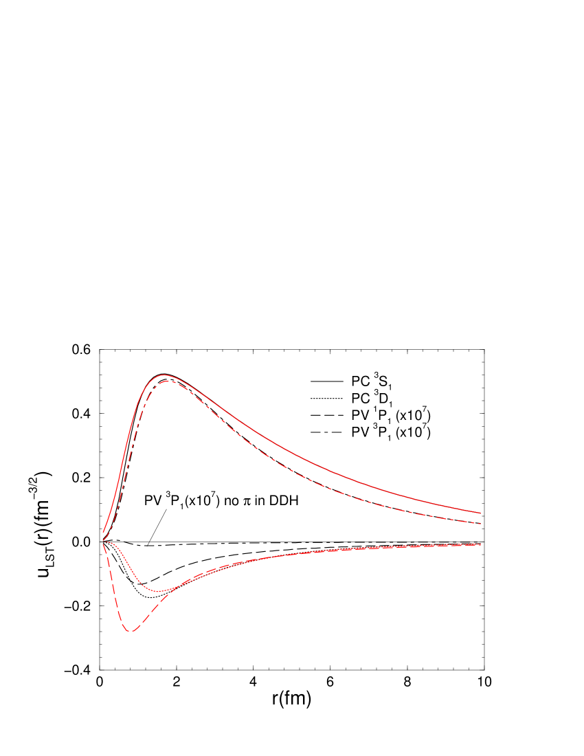
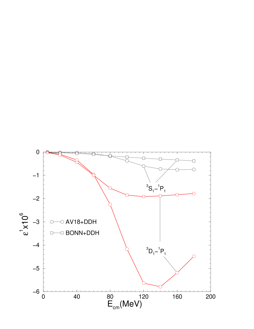
Figure 1 displays the functions obtained with the PC AV18 [9] (BONN [11]) and PV DDH [8] potentials (the values for the coupling constants and cutoff parameters in the DDH potential are those listed in Table I). The PC 3S1 and 3D1 components are not very sensitive to the input PC potential. For example, most of the difference between the AV18 and BONN 3D1 waves is due to non-localities present in the one-pion-exchange (OPE) part of the BONN potential. In fact, it has been known for over two decades [35], and recently re-emphasized by Forest [36], that the local and non-local OPE interactions are related to each other by a unitary transformation. Therefore the differences between local and non-local OPE cannot be of any consequence for the prediction of observables, such as binding energies and electromagnetic form factors, provided, of course, that three-body interactions and/or two-body currents generated by the unitary transformation are also included—see Ref. [37] for a recent demonstration of this fact within the context of a calculation of the deuteron structure function and tensor observable based on the local AV18 and non-local BONN potentials and associated (unitarily consistent) electromagnetic currents. This point was also stressed in Ref. [6].
The PV 3P1 component is, in magnitude, much larger than the 1P1. This is easily understood, since the long-range -exchange term in the DDH potential is non-vanishing only for transitions in which =1, and therefore does not contribute in the 1P1 channel. In this channel, however, the DDH - and -exchange terms play a role. Note that, because of the short-range character of the associated dynamics, the AV18 and BONN 1P1 waves show considerably more model-dependence than the corresponding 3P1 waves.
Finally, in Fig. 1 the PV 3P1 wave obtained with the AV18 and a truncated DDH potential, retaining only the short-range - and -exchanges, is also shown. The comparison between the 3P1 waves corresponding to the full and truncated DDH potentials demonstrates that this channel is indeed dominated by the -exchange term in the DDH.
V Parity-Violating Observables
In this section we give explicit expressions for parity-violating (PV) observables in the system, including the longitudinal asymmetry and spin rotation in elastic scattering, the photon asymmetry in radiative capture, and the asymmetries in deuteron photo-disintegration in the threshold region and electro-disintegration in quasi-elastic kinematics.
A Longitudinal asymmetry and spin rotation in elastic scattering
The differential cross section for scattering of a neutron with initial polarization is given by
| (76) |
and the longitudinal asymmetry is defined as
| (77) |
where denote the initial polarizations . The total asymmetry , integrated over the solid angle, then reads
| (78) |
where is the spin-averaged differential cross section. The optical theorem allows to be simply expressed as
| (79) | |||||
| (80) |
where in the equation above use has been made of the symmetry property
| (81) |
It is clear that the numerator of would vanish in the absence of PV interactions, since , in contrast to , cannot change the total spin or isospin of the pair. In particular, the long-range part of due to pion exchange can only contribute to the first term in the numerator of Eq. (80), since it is diagonal in , but non-vanishing for transitions =1.
The transmission of a low-energy neutron beam through matter is described in terms of an index of refraction. A heuristic argument, outlined in Ref. [38], and the more rigorous—although less transparent—derivation presented in Ref. [33] show that a neutron with spin projection , after traversing a slab of width of matter, is described by an asymptotic wave function given by
| (82) |
where = is the initial relative momentum (assumed along the -axis), and the index of refraction is related to the density of scattering centers in matter and the forward scattering amplitude. For the specific case under consideration here—neutron scattering from hydrogen—this relation reads:
| (83) |
Thus a neutron, initially polarized in the -direction,
| (84) |
having traversed a slab of matter, is described in the asymptotic region by a wave function given by
| (85) |
In the absence of , the difference vanishes, since it is proportional to the sum over in the numerator of Eq. (80), while
| (86) |
where is the spin-averaged cross section introduced above, and hence there will be an attenuation in the beam flux proportional to exp(). The real part of instead generates an un-observable phase factor.
B Photon asymmetry in radiative capture
In the center-of-mass (CM) frame, the radiative transition amplitude between an initial continuum state with neutron and proton in spin-projection states and , respectively, and in relative momentum , and a final deuteron state in spin-projection state , recoiling with momentum , is given by
| (88) |
where is the momentum of the emitted photon and , , are the spherical components of its polarization vector, and is the nuclear electromagnetic current operator. Note that has been taken along the -axis, the spin-quantization axis.
The initial continuum state, satisfying outgoing-wave boundary conditions, is related to that constructed in Sec. IV A via
| (89) | |||||
| (90) |
where in the first line the factor is from a Clebsch-Gordan coefficient combining the neutron and proton states to total isospin , and in the second line and the states have wave functions
| (91) |
with = and similarly for . The quantum numbers and characterize the incoming and outgoing waves, respectively.
The CM differential cross-section for capture of a neutron with spin projection is then written as
| (92) |
where is the angle between and and
| (93) |
Here is the fine-structure constant, is the deuteron mass, is the relative velocity, , and the photon energy is given by
| (94) |
The photon asymmetry is defined as in Eq. (77) with replaced by . By expanding the matrix elements of the current operator in terms of reduced matrix elements (RMEs) of electric () and magnetic () multipole operators as [28]
| (96) | |||||
with
| (97) |
and = or , one finds, by retaining the 1S0 and 3S1 channels in the sum over in Eq. (90), the only relevant incoming waves in the energy regime of interest here (fractions of eV),
| (98) |
where is given by
| (99) |
and in Eq. (96) the are standard rotation matrices [42]. The and RMEs should carry a superscript ; it has been dropped for ease of presentantion.
Several comments are now in order. Firstly, the photon asymmetry has the expected dependence on , since . Note that the contributions of higher order multipole operators with =2 have been ignored in the equation above.
Secondly, because of the definition of the states in Eq. (91), a generic RME is expressed as
| (100) |
namely as a sum over the contributions of outgoing channels corresponding to an incoming channel ; for example,
| (101) |
Thirdly, in the absence of parity-violating interactions, the only surviving RMEs are the , , and , and therefore the parameter vanishes. Furthermore, the RME also vanishes due to orthogonality of the initial and final states (in the limit in which isoscalar two-body currents are neglected), while the RME is suppressed in the energy regime of interest here. Thus, the standard result for the spin-averaged radiative capture cross-section, integrated over the solid angle, follows:
| (102) |
Lastly, when PV interactions are present, the analysis is more delicate, since then, in addition to ad-mixing small opposite-parity components into the wave functions corresponding to , these interactions also induce two-body terms in the electromagnetic current operator, as discussed in Sec. III. Thus, =, where includes the convection and spin-magnetization currents of single nucleons as well as the two-body currents associated with , while includes those terms generated by . The multipole operators can then be written as =, and those constructed from have un-natural parities, namely for and for . Therefore, for example, the RMEs and connect the PC 1S0 state to, respectively, the PC and PV components of the deuteron. A straight-forward analysis then shows that, up to linear terms in effects induced by either in the wave functions or currents, the parameter is given by
| (103) |
where again terms containing the RMEs and have been neglected. In the expression above, the RME has also been neglected, since transitions induced by the isoscalar electric dipole operator are strongly suppressed [43, 44]. Thus, the only relevant transitions are those connecting the 3P1 PV state to the PC deuteron component and the 3S1 and 3D1 PC states to the 3P1 PV deuteron component.
C Helicity-dependent asymmetry in photo-disintegration
The relevant matrix element in the photo-disintegration of a deuteron initially at rest in the laboratory is
| (104) |
in the notation of Sec. V B above. Here represents an scattering state with total momentum and relative momentum , satisfying incoming wave boundary conditions. Its (internal) wave function has the same partial wave expansion given in Eq. (40), except for the replacement .
The cross section for absorption of a photon of helicity , summed over the final states and averaged over the initial spin projections of the deuteron, reads:
| (105) | |||||
| (106) |
where is the energy of the final state,
| (107) |
and
| (108) |
Note that the factor 1/2 above is introduced to avoid double-counting the final states, and that the dependence upon the boundary condition of the continuum wave functions, the superscript , has been reinserted in the RMEs of the electric and magnetic multipoles, namely
| (109) |
and = or .
The resulting PV asymmetry, defined as , is expressed as
| (110) |
and therefore vanishes unless (i) the initial and/or final states do not have definite parity (as is the case here because of the presence of PV interactions) and/or (ii) the electric and magnetic multipole operators have unnatural parities and , respectively, because of two-body PV electromagnetic currents associated with PV interactions [7].
It is easily shown that in the inverse process the expression for the photon circular polarization parameter is identical to that given above, but for the RMEs and being replaced by the corresponding and , defined in the previous section. Indeed, by making use of the transformation properties of the states and electric and magnetic multipole operators under time reversal ,
| (111) | |||||
| (112) | |||||
| (113) |
one finds the following relation for the RMEs:
| (114) |
and similarly for the ’s. Hence, the circular polarizations measured in the direct and inverse processes are the same.
D Longitudinal asymmetry in electro-disintegration
The longitudinal asymmetry in the inclusive scattering of polarized electrons off a nuclear target results from the interference of amplitudes associated with photon and exchanges as well as from the presence of parity-violating components in the nucleon-nucleon interaction. For completeness, we summarize below the relevant formulae. The initial and final electron (nucleus) four-momenta are labeled by and ( and ), respectively, while the four-momentum transfer is defined as . The amplitudes for the - and -exchange processes are then given by [45]
| (115) | |||||
| (116) | |||||
| (117) |
where is the Fermi constant for muon decay, and are the Standard Model values for the neutral-current couplings to the electron given in terms of the Weinberg angle , and are the initial and final electron spinors, and and denote matrix elements of the electromagnetic and weak neutral currents, i.e.
| (118) |
and similarly for . Here and represent the initial deuteron state and final scattering state with incoming-wave boundary conditions (the solution), respectively. Note that in the amplitude the dependence of the propagator has been ignored, since .
The parity-violating asymmetry is given by the ratio of the difference over the sum of the inclusive cross sections for incident electrons with helicities . It depends on the three-momentum and energy transfers, and , and scattering angle, , of the electron and conveniently expressed
| (119) |
Standard manipulations then lead to the following expression for the asymmetry in the extreme relativistic limit for the electron [31, 45]
| (120) | |||||
| (121) |
where the ’s are defined in terms of electron kinematical variables,
| (122) | |||||
| (123) | |||||
| (124) |
The ’s are the nuclear electro-weak response functions, which depend on and , to be defined below. To this end, it is first convenient to separate the weak current into its vector and axial-vector components, and to write correspondingly
| (125) |
The response functions can then be expressed as
| (126) | |||||
| (127) | |||||
| (128) |
where is the ground-state energy of the deuteron (assumed at rest in the laboratory), is the energy of the final scattering state, and in Eqs. (126) and (127) [Eq. (128)] the superscript () is either or ( or 5). Note that there is a sum over the final states and an average over the initial spin projections of the deuteron. In the expressions above for the ’s, it has been assumed that the three-momentum transfer is along the -axis, which defines the spin quantization axis for the nuclear states.
The asymmetry induced by hadronic weak interactions, , is easily seen to be proportional to the interference of electric and magnetic multipole contributions as in Eq. (110), indeed
| (129) |
namely is related, of course for =, to the difference of helicity-dependent photo-disintegration cross sections. Similar considerations to those in Sec. V C allow one to conclude that this response would vanish in the absence of PV interactions (note, however, that in the present case there is, in addition to two-body PV currents, also a one-body PV term originating from radiative electro-weak corrections, the anapole current [23]).
VI Calculation
In this section we briefly review the techniques used to calculate the PV observables in the system—these are similar to those discussed most recently in Ref. [31].
The deuteron wave function in Eq. (70) is written, for each spatial configuration , as a vector in the spin-isospin space of the two nucleons,
| (130) |
where and are the components of in this basis. The scattering wave function in Eq. (40) is first approximated by retaining PC and PV interaction effects in all channels up to a certain pre-selected and by using spherical Bessel function for channels with , and is then expanded, for any given , in the same basis defined above. The radial functions are obtained with the methods discussed in Sec. IV C.
Matrix elements of the electromagnetic (and neutral-weak) current operators are written schematically as
| (131) |
The spin-isospin algebra is performed exactly with techniques similar to those developed in Ref. [17], while the -space integrations are carried out efficiently by Gaussian quadratures. Note that no multipole expansion of the transition operators is required.
Extensive and independent tests of the computer programs have been completed successfully.
VII Results and Discussion
In this section we present results for the longitudinal asymmetry and spin rotation in elastic scattering, the photon asymmetry in the radiative capture at thermal energies, and the asymmetries in the threshold photo-disintegration and quasi-elastic electro-disintegration of the deuteron. To provide an estimate for the model dependence of these results, we consider several different high-quality interactions fit to strong-interaction data, the Argonne (AV18) [9], Bonn (BONN) [11] and Nijmegen-I (NIJM-I) [10] interactions. We adopt the standard DDH [8] one-boson exchange model of the parity-violating (PV) interaction, and solve the Schrödinger equation for the scattering state and deuteron bound state with the methods discussed in Sec. IV. The values for the meson-nucleon coupling constants and cutoff parameters in the DDH model are those listed in Table I. Note that we have taken the linear combination of - and -meson weak coupling constants corresponding to elastic scattering from an earlier analysis [6] of these experiments. The remaining couplings are the DDH “best value” estimates. As in the earlier analysis of scattering, the cutoff values in the meson-exchange interaction are taken from the BONN potential.
It is also useful to introduce here some of the notation adopted in the following subsections to denote variations on the DDH model defined above. The PV interaction denoted as DDHb corresponds to a DDH model with , and weak coupling constants as specified by the “best value” set of Ref. [8], while the PV interaction denoted as DDH includes only the -exchange term in the DDH model with the “best value” for the weak coupling constant. The remaining pion and vector-meson strong interaction coupling constants and short-range cutoff parameters are as given in Table II for the DDHb model and are the same as in Table I for the DDH model.
Finally, while the short-range contributions to the PV interaction should not be viewed as resulting solely from the exchange of single mesons, the six parameters of the DDH model are still useful in characterizing all the low-energy PV mixings. For example, two-pion exchange could play a role [46], however we assume that its effects can be included, at least at low energy, through the present combination of pion- and short-range terms.
A Longitudinal asymmetry and neutron spin rotation
In this section we present results for the longitudinal asymmetry and neutron spin rotation in elastic scattering.
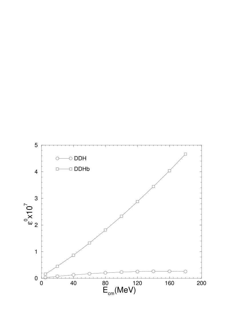
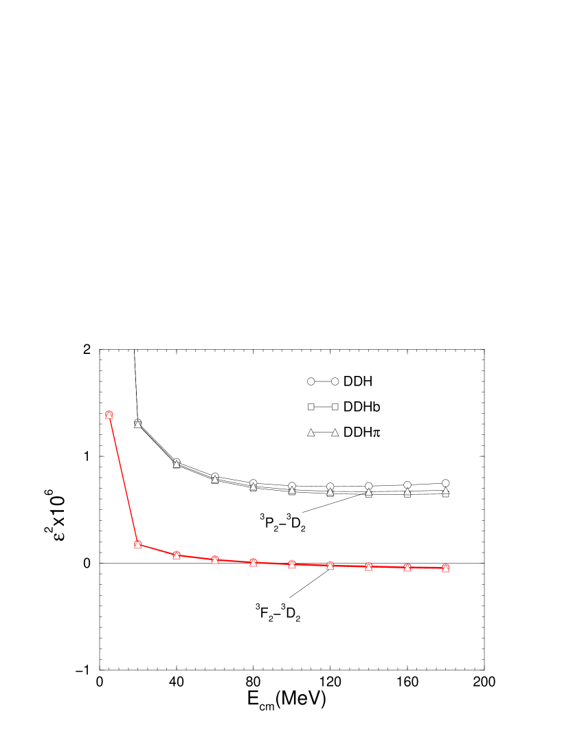
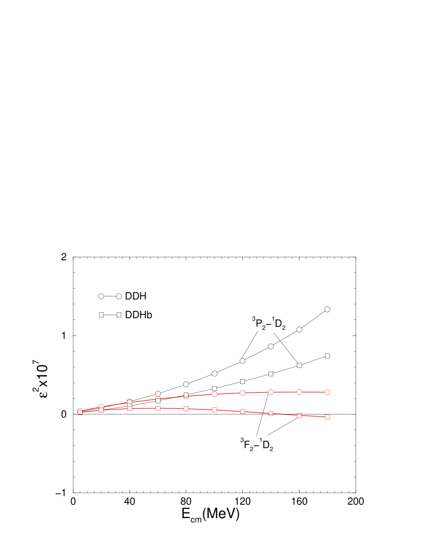
Figures 3–7 show the mixing parameters induced by AV18 model in combination with the DDH, DDHb, and DDH interactions. Only those induced by the PV interaction are displayed, namely for =0 and for with =1,2 and =3,4 in the notation of Tables III and IV.
The definitions adopted for the phase-shifts and mixing parameters are those introduced in Sec. IV B. Up to linear terms in , the and values are not affected by weak interactions, and are determined solely by the strong interaction. They are identical to those listed in Ref. [9], but for two differences. Firstly, the Blatt-Biedenharn parameterization is used here for the -matrix [47] rather than the bar-phase parameterization of it [48] employed in Ref. [9]. Secondly, because of the phase choice in the potential components (see Eq. (46) and comment below it), the mixing parameters have opposite sign relative to those listed in Ref. [9].
The coupling between channels with the same pair isospin is induced by the short-range part of the DDH interaction, associated with vector-meson exchanges; its long-range component, due to pion exchange, vanishes in this case. As a result, the mixing parameters in Figs. 3, 5, and 7, calculated with the DDH and DDHb models, are rather different, reflecting the large differences in the values for the some of the strong and weak coupling constants and short-range cutoffs between these two models, see Tables I and II.
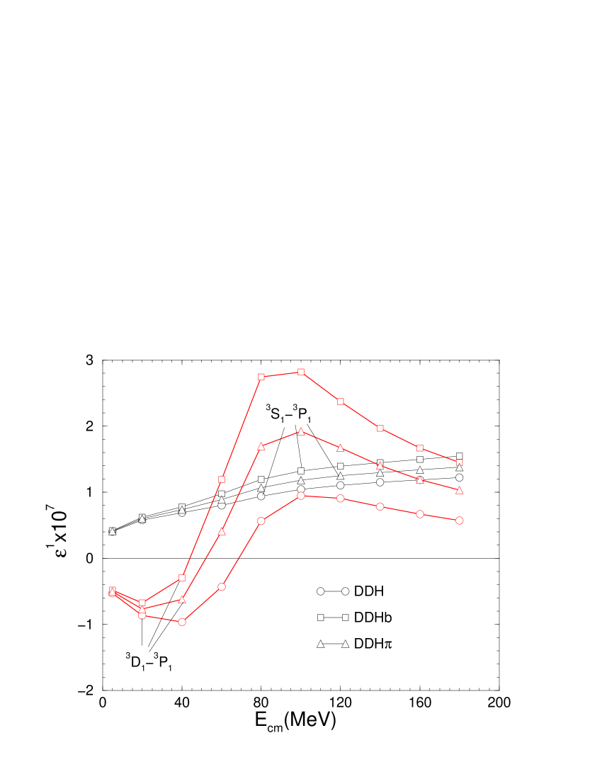
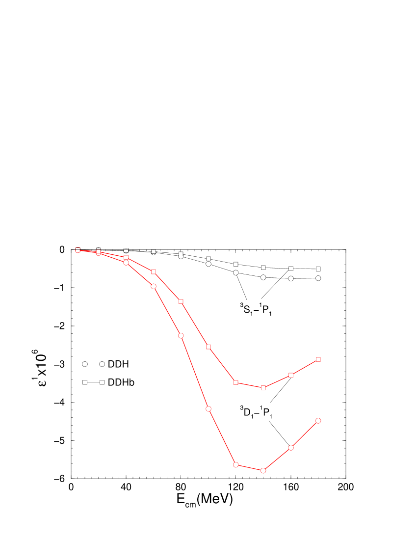
The mixing parameters between channels with =1, Figs. 4 and 6, in which the pion-exchange term is present, are still rather sensitive to the short-range behavior of the PV interaction, as reflected again by the differences in the DDH and DDHb predictions. However, this sensitivity is much reduced for the more peripheral waves, such as the 3P2-3D2 and 3F2-3D2 channels.
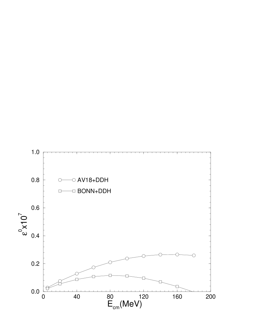
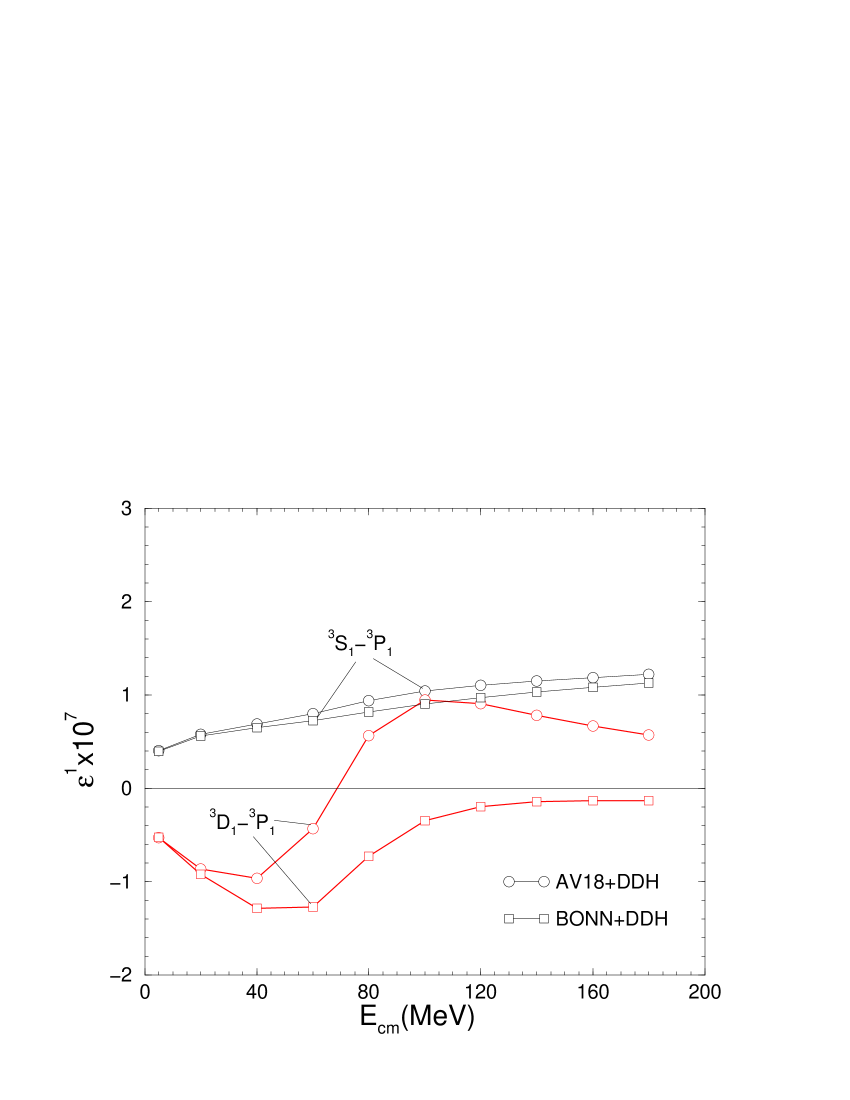
Figures 8–10 are meant to illustrate the sentitivity of the mixing angles to the input strong-interaction potential, which can be quite large, particularly in channels, such as the 3D1-1P1.
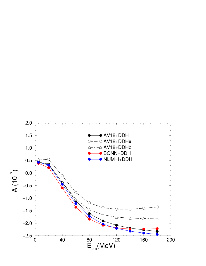
The total longitudinal asymmetry, defined in Eq. (78), is shown in Fig. 11 for a number of combinations of strong- and weak-interaction potentials. The asymmetries were calculated by retaining in the partial wave expansion for the amplitude, Eq. (60), all channels with up to =6. There is very little sensitivity to the input strong-interaction potential. As also remarked in Ref. [6], this reduced sensitivity is undoutbly a consequence of the fact that present potentials are fitted to extended and databases with high accuracy.
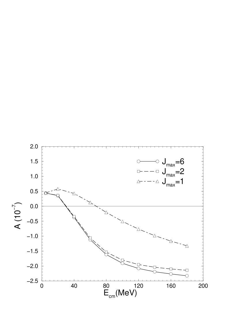
Figure 12 shows that the total asymmetries obtained by including only the =0 and 1 channels (1S0-3P0, 3S1-3P1, 3D1-3P1, 3S1-1P1, and 3D1-1P1) and, in addition, the =2 channels, and finally all channels up to =6. In the energy range (0–200) MeV the asymmetry is dominated by the =0–2 contributions.
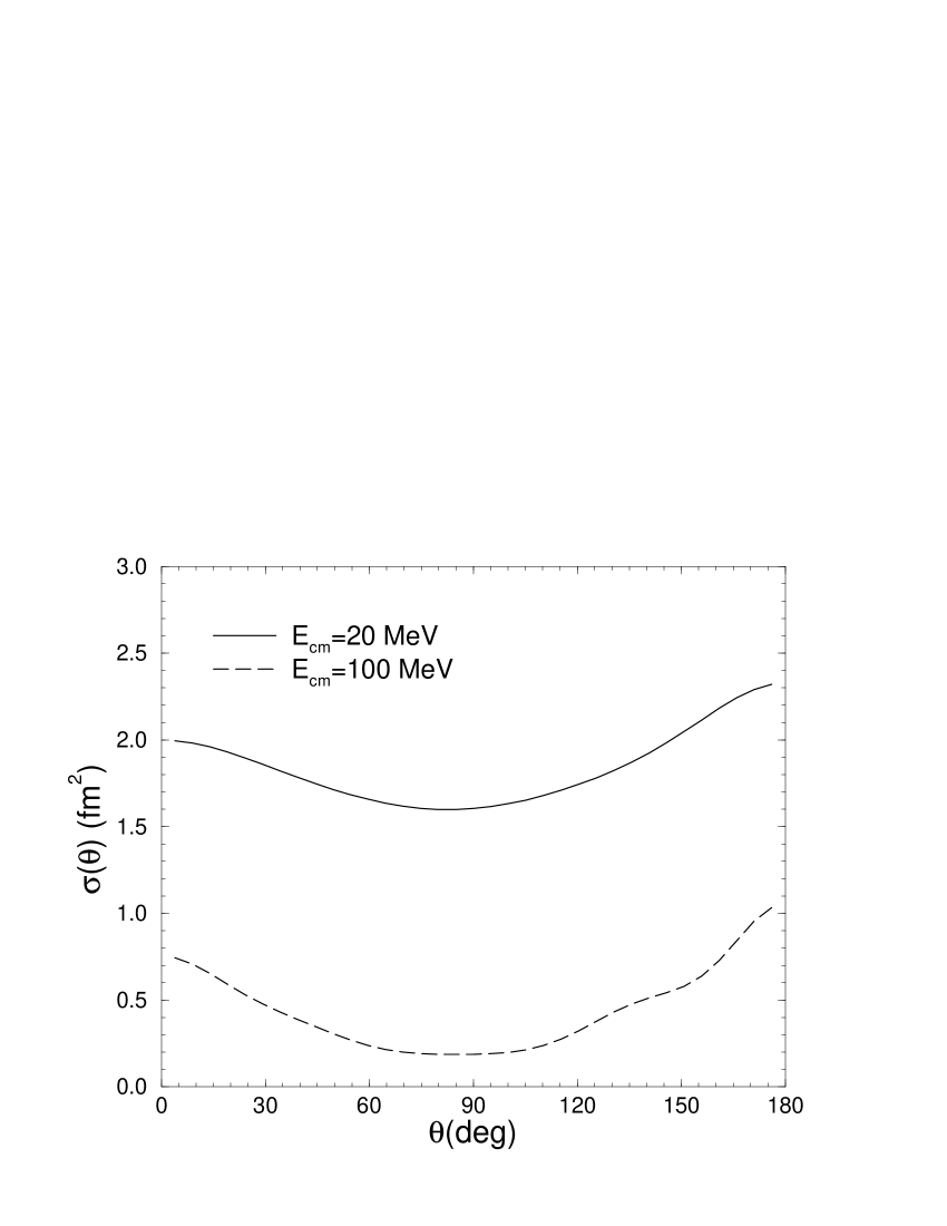
For completeness, we present in Figs. 13 and 14 results for the angular distributions of the (PC) spin-averaged differential cross section and (PV) longitudinal asymmetry at center-of-mass energies of 20 MeV and 100 MeV. The asymmetry is defined in Eq. (77).
The predictions for the neutron spin rotation per unit length, with defined in Eq. (87), are listed in Table V in the limit of vanishing incident neutron energy. The density of liquid hydrogen is taken as = atoms-cm-3.
While results corresponding to different input strong interactions are within 10% of each other, the calculated values show significant sensitivity to the short-range bahavior of the PV interaction, columns labeled DDH and DDHb. It is worth re-emphasizing that the longitudinal asymmetry in elastic scattering predicted by the DDHb model is at variance with that observed experimentally [6]. The short-range cutoff parameters and combinations of - and -meson PV coupling constants in =11, respectively and , were constrained, in the DDH model, to reproduce this (measured) asymmetry [6]. An additional difference between the DDH and DDHb models is in the values adopted for the (PC) -meson tensor coupling to the nucleon, 6.1 in the DDH (from the BONN interaction) and 3.7 in the DDHb (consistent with estimates from vector-meson dominance). Hence, the DDHb results are not realistic. Comparison between the DDH and DDH predictions, however, indicates that the neutron spin rotation is sensitive to the long-range part of , and therefore a measurement of this observable would be useful in constraining the PV coupling constant.
Finally, there is a sign difference between the present results and those reported in Ref. [41]. It is not due to the different strong interaction potential used in that calculation. Indeed, with the Paris potential [49] in combination with the DDHb model we obtain = rad-cm-1, the same magnitude but opposite sign than given in Ref. [41].
In order to understand this discrepancy, we have carried out a calculation of the neutron spin rotation, which ignores strong-interaction effects. It is equivalent to a first-order (in ) perturbative estimate of this observable, and the corresponding results, listed in the last row of Table V (row labeled “plane waves”), demonstrate that strong-interaction distorsion effects are crucial, in fact they are responsible for flipping the sign of . This is in contradiction with the statement reported in the first paragraph after Eq. (6) of Ref. [41]: Avishai and Grange claim that the “plane-wave” prediction with the DDHb model is rad-cm-1, namely it has the same sign as in their full calculation.
The sign difference between the predictions obtained by either including or neglecting strong-interaction distorsion effects can easily be understood. For simplicity, consider the DDH model, in which case the relevant matrix element contributing to is PS, connecting the continuum =0 3S1 and =1 3P1 channels. The essential difference between the un-distorted and distorted 3S1 wave functions is the presence of a node in the latter, thus ensuring its orthogonality to the deuteron 3S1 component. It is this node that causes the sign flip.
B Photon asymmetry in radiative capture at low energies
The PV asymmetry in the 1H(,)2H reaction at thermal neutron energies is calculated for the AV18, BONN and NIJM-I interactions. The asymmetry is expected to be constant for low-energy neutrons up to energies well beyond the 1–15 meV averaged in the experiment currently running at the LANSCE facility [50]. Each strong interaction model has associated two-body currents. For the AV18 we consider the currents from the momentum-independent terms—the - and -exchange currents from its part—as well as from the momentum-dependent terms, as reviewed in Sec. III. Further discussion of the AV18 currents is given below. For the BONN and NIJM-I interactions, we retain only the - and -exchange currents with cutoff parameters taken from the BONN model (=1.72 GeV and =1.31 GeV), while we neglect contributions from other meson exchanges. In all calculations, however, the currents associated with the excitation and transition have been included.
The total cross section is due to the well-known transition connecting the PC 1S0 state to the PC deuteron state. The calculated values for each model are given in Table VI, both for one-body (impulse) currents alone and for the one- and two-body currents. In each case the largest two-body contribution, approximately two-thirds of the total, comes from the currents associated with pion exchange. The total cross section is in good agreement with experimental results, which are variously quoted as 334.2(0.5) mb [51] or 332.6(0.7) mb [52]. It would be possible to adjust, for example, the transition magnetic moment of the -excitation current to precisely fit one of these values, here we simply choose a of 3 n.m., which is consistent with an analysis of - data at resonance.
As discussed Sec. V B, the PV asymmetry arises from an interference between the term above and the transition, connecting the 3P1 PV state to the PC deuteron state and the 3S1 PC state to the 3P1 PV deuteron state. The transitions proceeding through the PV 1P1 or deuteron states are suppressed, because of an isospin selection rule forbidding isoscalar electric-dipole transitions and also because of spin-state orthogonality. In principle, there is a relativistic correction to the electric dipole operator, associated with the definition of the center-of-energy [44]. However, its contribution in transitions proceeding through the 1P1 channel vanishes too, since the associated operator is diagonal in the pair spin.
The calculated asymmetries are listed in Table VI. The results are consistent with earlier [53, 54] and more recent [55, 56] estimates, and are in agreement with each other at the few-per-cent level, which is also the magnitude of the contributions from the short-range terms. In particular, they show that this observable is very sensitive to the weak PV coupling constant, while it is essentially unaffected by short-range contributions (in this context, see also Fig. 1). The transition has been calculated in the long-wavelength approximation (LWA) with the Siegert form of the operator (see, for example, Eq. (4.5) of Ref. [43]), thus eliminating many of the model dependencies and leaving only simple (long-range) matrix elements. In the notation of Sec. V B, the associated reduced matrix elements (RMEs) are explicitly given by
| (132) | |||||
| (133) |
where the ’s and ’s denote the continuum and deuteron radial wave functions defined, respectively, as in Secs. IV A and IV D (only the outgoing channel quantum numbers are displayed for the ’s). Corrections beyond the LWA terms in transitions have been found to be quite small. For completeness, we also give the well known expression for the RME, as calculated to leading order in and in the limit in which only one-body currents are retained,
| (134) |
where the combination =4.706 n.m. is the nucleon isovector magnetic moment.
We have also calculated the contributions with the full current density operator , namely by evaluating matrix elements of
| (135) |
where are standard vector spherical harmonics. To the extent that retardation corrections beyond the LWA of the operator are negligible [43], this should produce identical results provided the current is exactly conserved. In order to satisfy current conservation, currents from both the strong (PC) and weak (PV) interactions are required, as discussed in Sec. III. In the following we keep only the -exchange term in the DDH interaction (with their “best guess” for the weak coupling constant), and use the AV18 strong-interaction model.
As reviewed in Sec. III, the PC two-body currents constructed from the part of the AV18 interaction (the - and -exchange currents) exactly satisfy current conservation with it. The same holds true for the PV -exchange currents derived from the DDH interaction in Sec. III A. However, the PC two-body currents originating from the isospin- and momentum-dependent terms of the AV18 are strictly not conserved (see below). The associated contributions, while generally quite small, play here a crucial role because of the large cancellation between the (PC) currents from the AV18 and the (PV) -currents from the DDH. This point is illustrated in Table VII. Note that the PC currents from -excitation and transition are transverse and therefore do not affect the matrix element. However, they slightly reduce the PV asymmetry, since their contributions increase the matrix element by %. They are not listed in Table VII.
The asymmetry is given by the sum of the two columns in Table VII, namely (last row). This value should be compared to , obtained with the Siegert form of the operator for the same interactions (and currents for the matrix element). As already mentioned, we have explicitly verified that retardation corrections in the operator are too small to account for the difference. Thus the latter is to be ascribed to the lack of current conservation, originating from the isospin- and momentum-dependent terms of the AV18.
To substantiate this claim, we have carried out a calculation based on a reduction [57] of the AV18 (denoted as AV8), constrained to reproduce the binding energy of the deuteron and the isoscalar combinations of the S- and P-wave phase shifts (note, however, that we do include in the AV8 the electromagnetic terms from the AV18, omitted in Ref. [57]). For the AV8 model, the - and -exchange currents from the isospin-dependent central, spin-spin, and tensor interaction components are constructed as for the AV18, and therefore are exactly conserved. However, the currents from the isospin-independent interaction, , are derived by minimal substitution,
| (136) |
where and are the electric charge and vector potential, respectively, and is the proton projection operator. The linear terms in are written as , and the resulting spin-orbit current density—or, rather, its Fourier transform—reads
| (137) |
In the case of the isospin-dependent terms, after symmetrizing , one obtains
| (138) |
where
| (139) |
While minimal substitution ensures that the current is indeed conserved for the isospin-independent interaction, i.e.
| (140) |
this prescription does not lead to a conserved current for the isospin-dependent one, since the commutator above generates an isovector term of the type
| (141) |
Physically, this corresponds to the fact that isospin-dependent interactions are associated with the exchange of charged particles, which an electromagnetic field can couple to. One can enforce current conservation by introducing an additional term [58], which in the case of is taken as
| (142) |
The results obtained for the total cross section and PV asymmetry with the AV8 and pion-only DDH interactions and associated (exactly conserved) currents are listed in Table VIII. A few comments are in order. Firstly, the cross section in impulse approximation is 30% smaller than predicted with the AV18 interaction. This is due to the fact that the singlet scattering length obtained with the AV8 (truncated) model is –19.74 fm, and so is about 15% smaller in magnitude than its physical value, –23.75 fm, reproduced by the AV18 within less than 0.1% [9].
Secondly, the enhancement of the cross section in impulse approximation due to (PC) two-body currents, 9.3%, is essentially consistent with that predicted with the AV18.
Lastly, the PV asymmetry obtained with the full currents is close to that calculated with the Siegert form of the operator. The remaning % difference is due to numerical inaccuracies as well as additional corrections from retardation terms and higher order multipoles. Both of these effects are included in the full-current calculation. Note the crucial role played by the spin-orbit currents constructed above.
C Deuteron threshold disintegration with circularly polarized photons
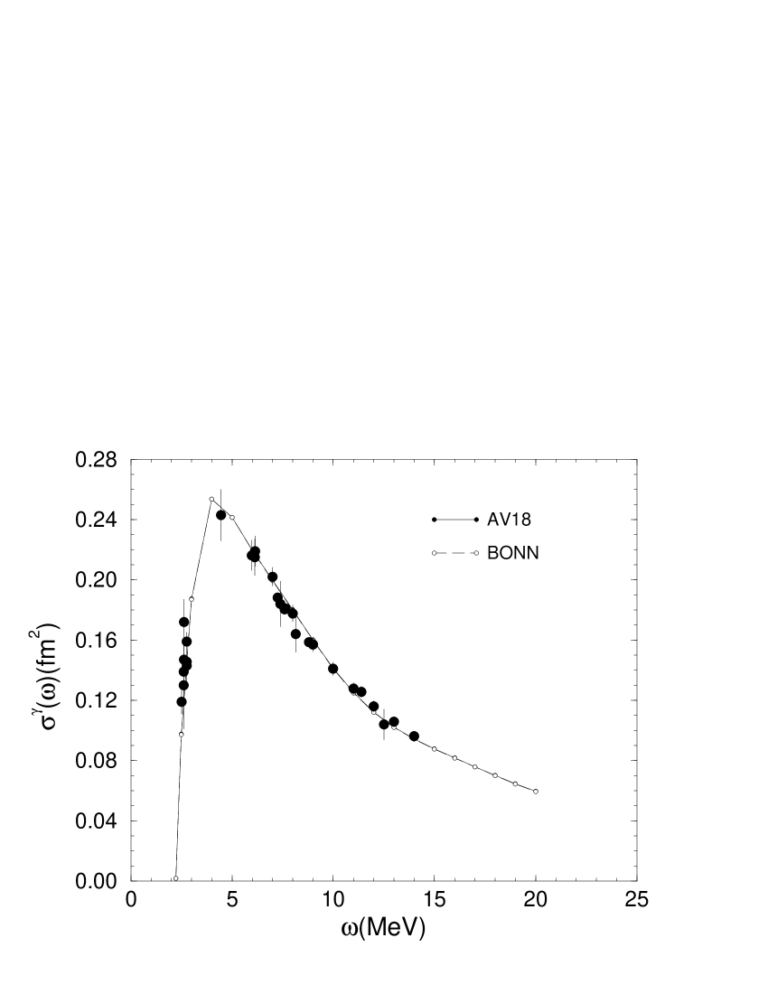
The photo-disintegration cross sections calculated with the AV18 and BONN models from threshold to 20 MeV photon energies are in excellent agreement with data [59]–[65], see Fig. 15. The model dependence between the AV18 and BONN results is negligible. In the calculations the final states include interaction effects in all channels up to =5 and spherical Bessel functions for , as discussed in the next section.
In the energy regime of interest here, the (total) cross section is dominated by the contributions of transitions connecting the deuteron to the triplet P-waves. The Siegert form is used for the operator. Because of the way the calculations are carried out (see Sec. VI), it is conveniently implemented by making use of the following identity for the current density operator , or rather its Fourier transform ,
| (143) | |||||
| (144) |
where in the first line the volume integral of has been re-expressed in terms of the divergence of the current, ignoring vanishing surface contributions, and in the second line use has been made of the continuity equation. Here is the charge density operator. In evaluating the matrix elements in Eq. (104) the commutator term reduces to
| (145) |
where is the proton projection operator introduced earlier, and relativisitc corrections to , such as those associated with spin-orbit and pion-exchange contributions [43, 44], have been neglected.
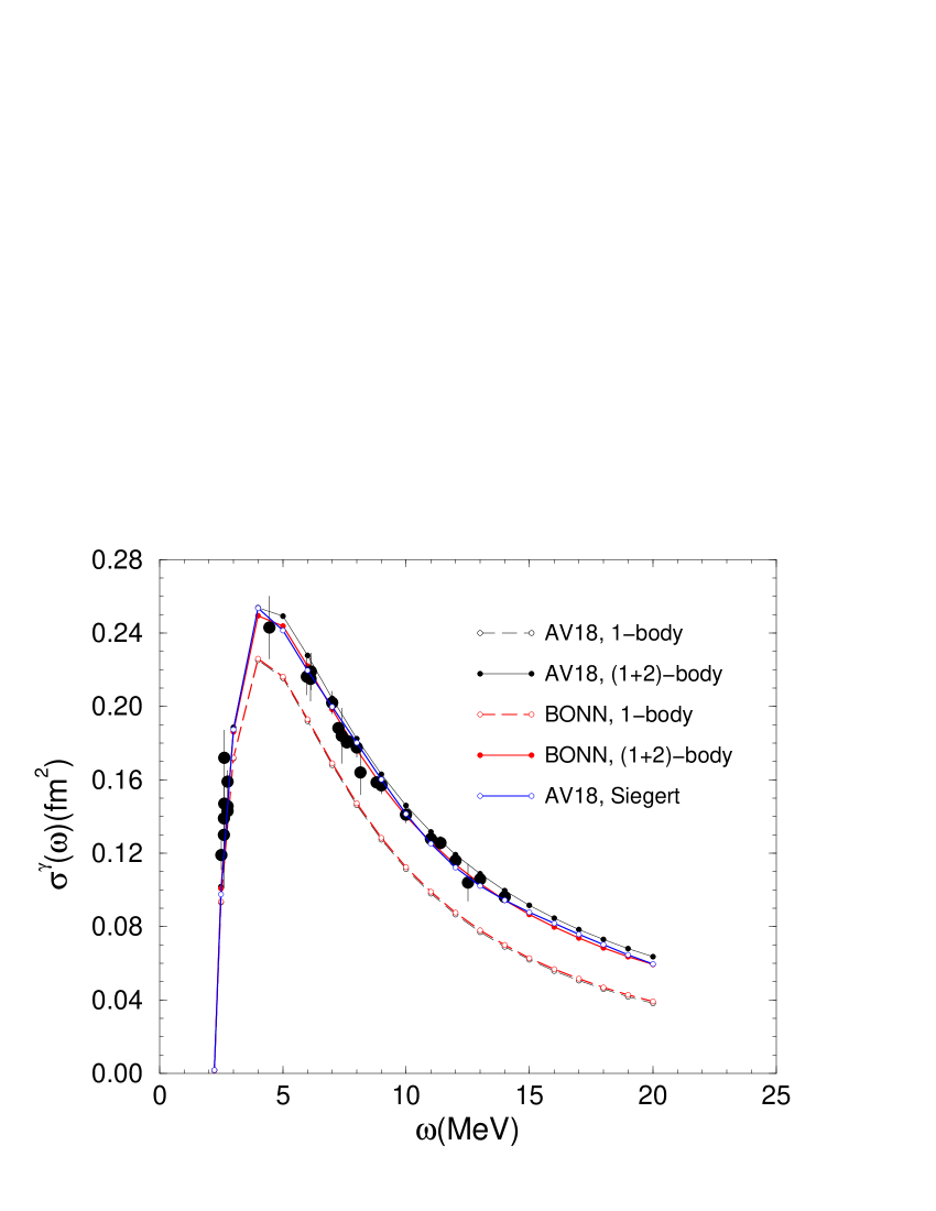
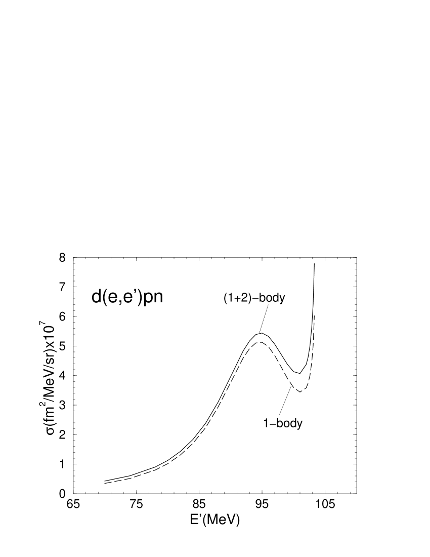
We have also calculated the photo-disintegration cross section by using the expression given in Eq. (135) for the operator, or equivalently by calculating matrix elements of the current without resorting to the identity in Eq. (144). The results obtained by including only the one-body terms and both the one- and two-body terms in are compared with those obtained in the Siegert-based calculation (as well as with data) in Fig. 16. The same conclusions as in the previous section remain valid here. Had the current been exactly conserved, then the Siegert-based and full calculations would have produced identical results. The small differences in the case of the AV18 model, as an example, are to be ascribed to missing isovector currents associated with its momentum-dependent interaction components (see previous section).
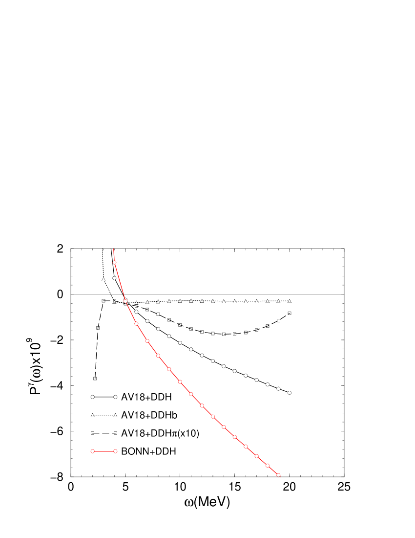
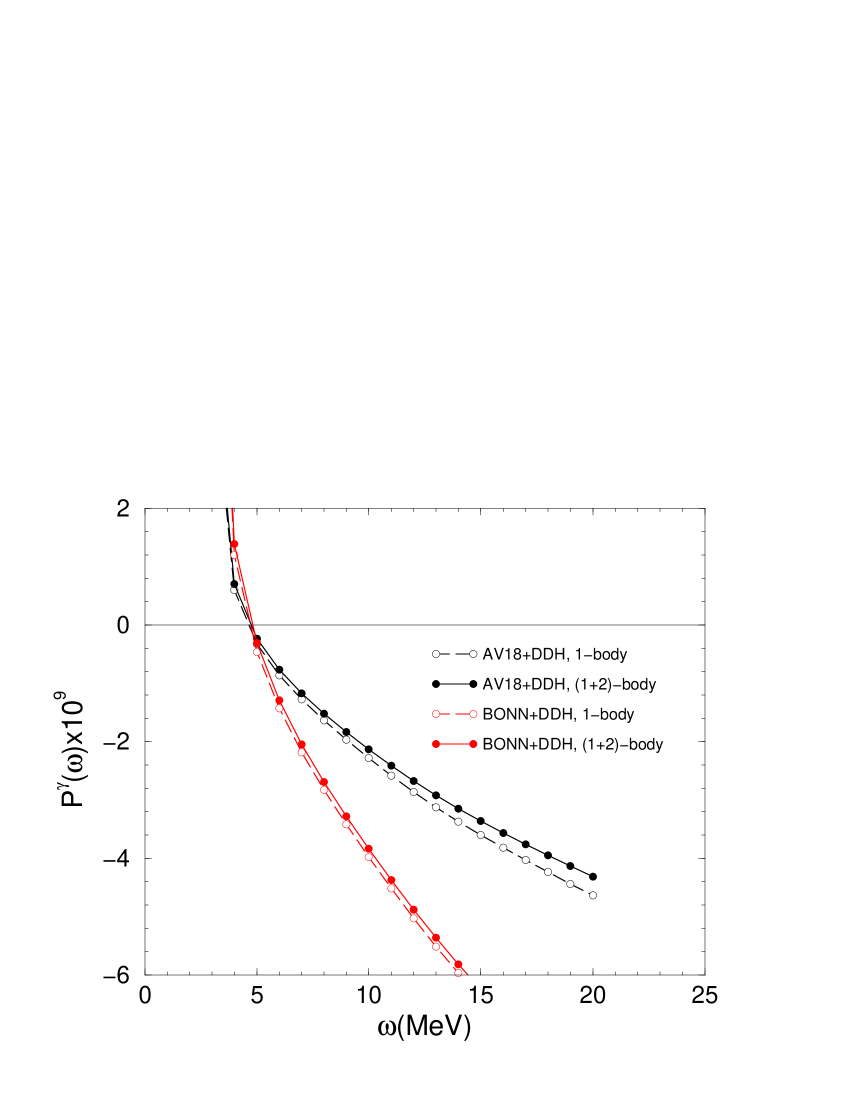
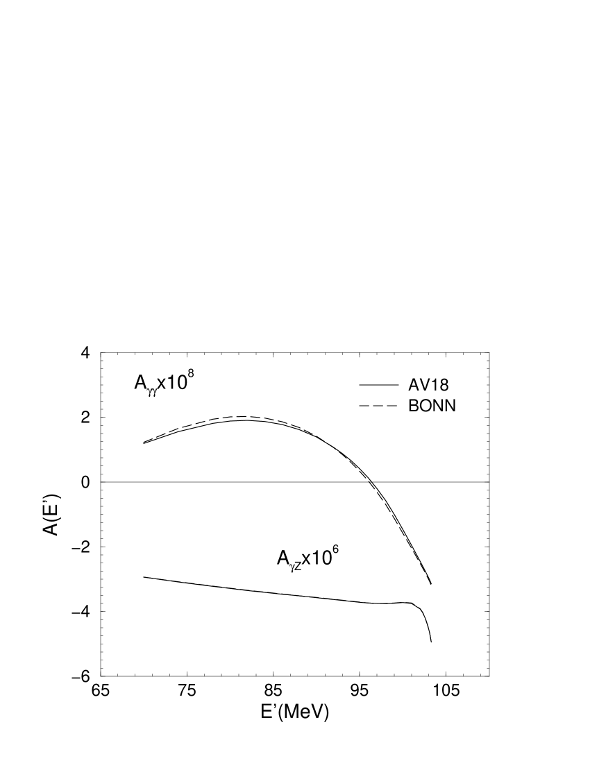
The PV photon polarization parameter , obtained with various combinations of PC and PV interactions, is displayed in Fig. 17, while its value at a photon energy 1.3 keV above breakup threshold is listed in Table IX. All results presented below use the current operator in the form given on the right-hand-side of Eq. (144). Note that, as discussed in Sec. V C, the parameters for the direct and inverse processes are the same. In the threshold region, a few keV above breakup, the expression for reduces to
| (146) |
where, in the notation of the previous section, the RME is defined as in Eq. (101) and similarly for . In this energy region, the only relevant channel in the final state has =0, see discussion at the end of Sec. V B. Note that the combination of RMEs occurring in is different from that in , the photon angular asymmetry parameter measured in radiative capture. Indeed, in contrast to , the photon polarization parameter is almost entirely determined by the short-range part of the DDH interaction, mediated by vector-meson exchanges (and having isoscalar and isotensor character [66]), see Table IX and Fig. 17. This is easily understood, since in the 1S0-3P0 channel the pion-exchange component of the DDH interaction vanishes. Furthermore, the transition connecting the 1S0 continuum state to the PV 3P1 component of the deuteron, which is predominantly induced by the pion-exchange interaction, is strongly suppressed, to leading order, by spin-state othogonality. Higher order corrections, associated with retardation effects and relativistic contribution to the electric dipole operator, were estimated in Ref. [67] and were found to be of the order of a few % of the leading result arising from vector-meson exchanges. Some of these corrections are retained in the present study.
The predictions in Table IX and in Fig. 17 display great sensitivity both to the strengths of the PV vector-meson couplings to the nucleon and to differences in the short-range behavior of the strong-interaction potentials, thus reinforcing the conclusion that these short-ranged meson couplings are not in themselves physical observables, rather the parity-violating mixings are the physically relevant parameters.
Note that the 5% decrease in values between the rows labelled “impulse” and “full” is due to the corresponding 5% enhancement of the transition connecting the PC 1S0 and deuteron states, due to two-body terms in the electromagnetic current included in the “full” calculation.
The results in Table IX are consistent both in sign and order of magnitude with those of ealier studies [68, 69, 70, 71], remaining numerical differences are to be ascribed to different strong- and weak-interaction potentials adopted in these earlier works. Indeed, we have explicitely verified that by using the PC AV18 potential and the Cabibbo model for the PV potential [72] we obtain values close to those reported in Ref. [70, 71]. However, our results seem to be at variance with those of Ref. [73] at photon energies a few MeV above above the breakup threshold. In particular, Table II in that paper suggests that at 10 and 20 MeV the dominant contribution to is from the PV pion-exchange interaction and that has the values and , respectively. This is in contrast to what reported in Fig. 17 of the present work, curves labelled AV18+DDHb and AV18+DDH. There is a two-order of magnitude difference between the values referred to above and those obtained here. It is not obvious whether this is due to the use in Ref. [73] of the Hamada-Johnston [74] PC potential—a PV potential “close” to our model DDHb is adopted.
The results in Table IX are consistent with the latest experimental determination, = [75], but about two orders of magnitude smaller than an earlier measurement [76].
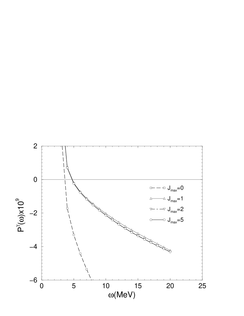
Figure 18 shows the photon-polarization parameter obtained by including PV admixtures in the continuum wave functions of all channels with and =0, 1, 2 and 5. In the energy range explored so far, is essentially given by the contributions of the =0 and 1 channels.
D Deuteron electro-disintegration at quasi-elastic kinematics
In this section we present results for the asymmetries and obtained by including one- and two-body terms in the electromagnetic and neutral-weak currents. Note, however, that only the PV two-body terms associated with -exchange in the DDH interaction are considered in the present calculations (in addition, of course, to the PC terms discussed in Sec. III). The PV currents from - and -exchange have been neglected, since they are expected to play a minor role due to their short-range character. One should also observe that at the higher momentum transfers of interest here, 100–300 MeV/c, relevant for the SAMPLE experiments [4, 77], it is not possible to include the contributions of electric multipole operators through the Siegert theorem, these must be calculated explicitly from the full current.
The contribution was recently studied in Ref. [31], where it was shown that two-body terms in the nuclear electromagnetic and weak neutral currents only produce (1–2)% corrections to the asymmetry due to the corresponding single-nucleon currents. The present study—a short account of which has been published in Ref. [7]—investigates the asymmetry originating from hadronic weak interactions. It updates and sharpens earlier predictions obtained in Refs. [78, 79]—for example, these calculations did not include the effects of two-body currents induced by PV interactions.
The present calculation proceeds as discussed in Sec. VI. We have used the AV18 or BONN models (and associated currents) in combination with the full DDH interaction (with coupling and cutoff values as given in Table I). The final state, labeled by the relative momentum , pair spin and -projection , and pair isospin (=0), is expanded in partial waves; PC and PV interaction effects are retained in all partial waves with , while spherical Bessel functions are employed for . In the quasi-elastic regime of interest here, it has been found that interaction effects are negligible for .
In Figs. 20 and 21 we show, respectively, the inclusive cross section and the asymmetries and , obtained with the AV18 and DDH interactions, for one of the two SAMPLE kinematics, corresponding to a three-momentum transfer range between 176 MeV and 206 MeV at the low and high ends of the spectrum in the scattered electron energy , the four-momentum transfer at the top of the quasi-elastic peak is 0.039 GeV2. The rise in the cross section at the high end of the spectrum—the threshold region—is due to the transition connecting the deuteron to the (quasi-bound) 1S0 state. Note that, because of the well-known destructive interference between the one-body current contributions originating from the deuteron S- and D-wave components, two-body current contributions are relatively large in this threshold region. However, they only amount to a 5% correction in the quasi-elastic peak region.
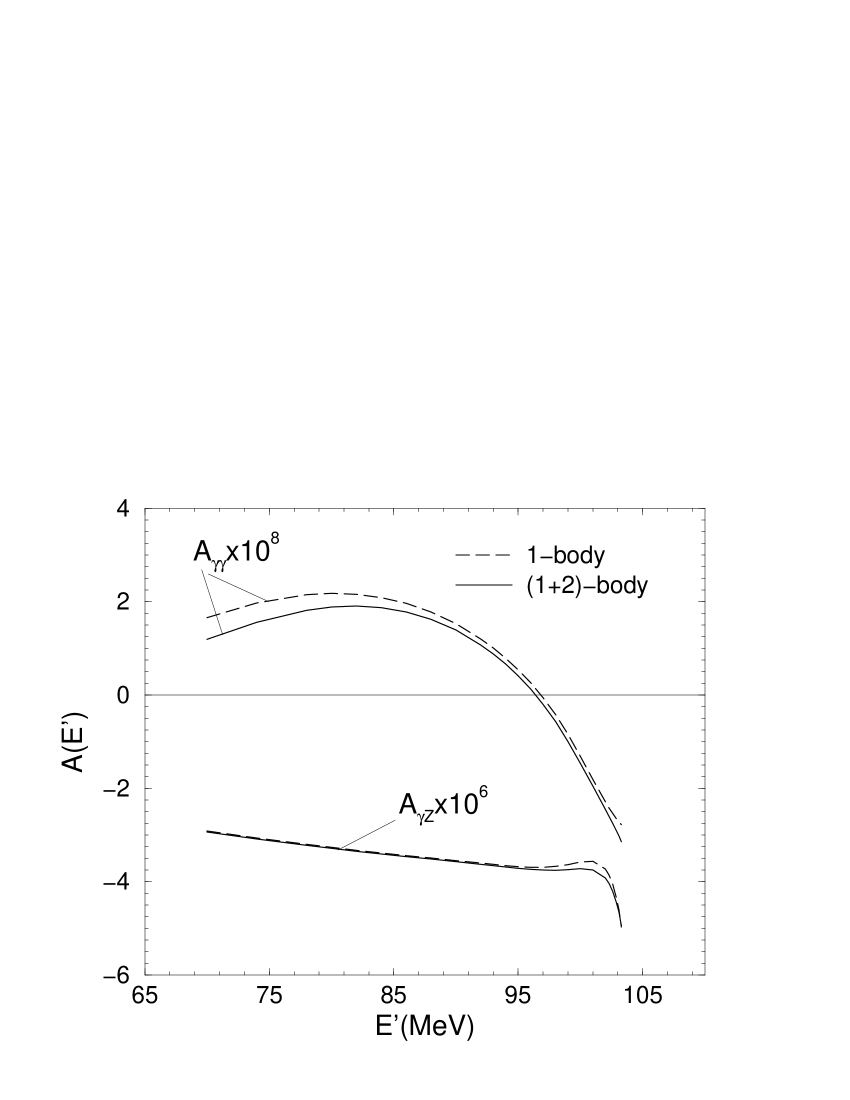
In Fig. 21 the asymmetry labeled (1+2)-body— is defined in Eq. (121)—includes, in addition to one-body, two-body terms in the electromagnetic and neutral weak currents (in both the vector and axial-vector components of the latter). These two-body contributions are negligible over the whole spectrum. However, the (PC and PV) two-body electromagnetic currents play a relatively more significant role in the asymmetry , Eq. (120).
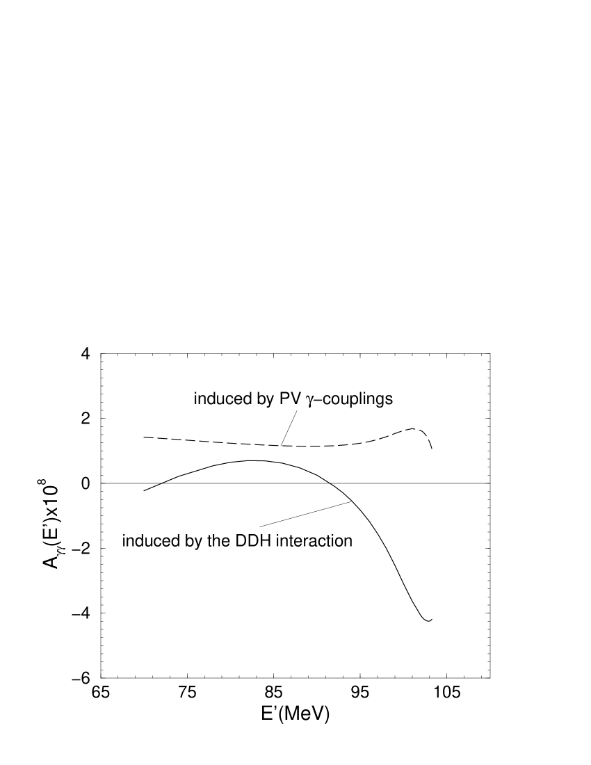
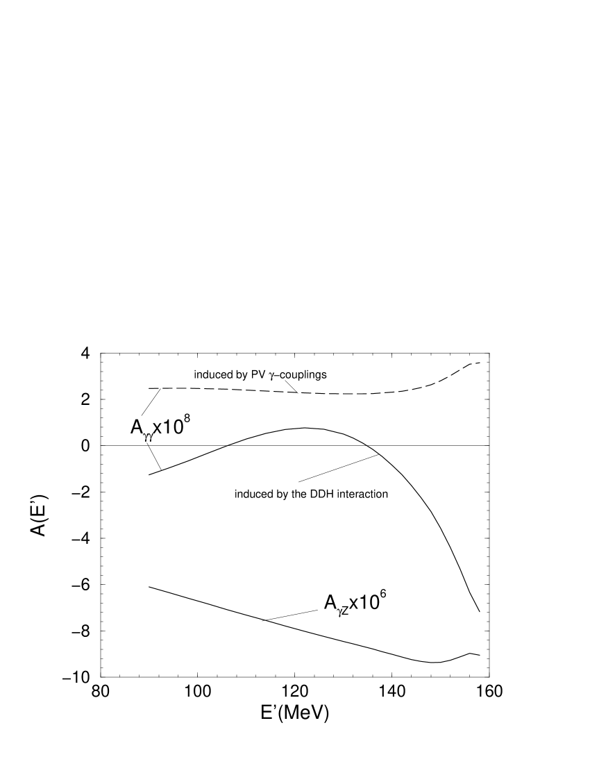
In Fig. 22 we display separately, for the asymmetry , the contributions originating from i) the presence in the wave functions of opposite-parity components induced by the DDH interaction (solid curve) and ii) the anapole current and the PV two-body current associated with -exchange (dashed curve). The latter are positive and fairly constant as function of , while the former exhibit a pronounced dependence upon . Note that, up to linear terms in the effects induced by PV interactions, the asymmetry is obtained as the sum of these two contributions.
The BONN model leads to predictions for the inclusive cross section and asymmetries, that are very close to those obtained with the AV18, as shown for and in Fig. 23. Thus the strong-interaction model dependence is negligible for these observables.
In Fig. 24 we present results for the asymmetries corresponding to a four-momentum transfer at the top of the quasi-elastic peak of about 0.094 GeV2, the three-momentum transfer values span the range (266–327) MeV over the spectrum shown. The calculations are based on the AV18 model and include one- and two-body currents. The asymmetry from - interference scales with and therefore is, in magnitude, about a factor of two larger than calculated in Fig. 21 where 0.039 GeV2. The contributions to exhibit, as functions of , a behavior qualitatively similar to that obtained at the lower value, see Fig. 22.
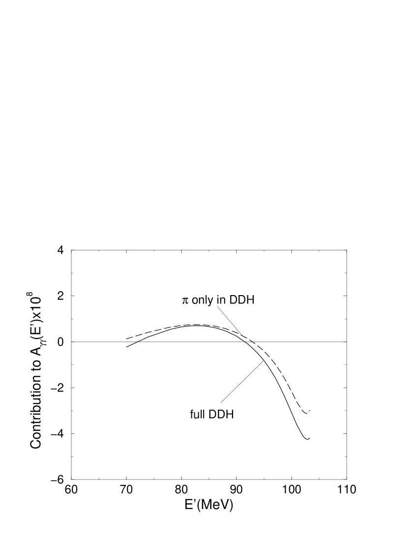
In Fig. 25 we compare results for the contribution to due to the presence in the wave function of opposite-parity components induced by the full DDH and a truncated version of it, including only the pion-exchange term. Note that, up to linear terms in the effects produced by PV interactions, the other contribution to , namely that originating from (PV) one- and two-body currents, remains the same as in Fig. 22, since—as mentioned earlier—only the (PV) two-body currents associated with pion-exchange are considered in the present work. Figure 25 shows that the asymmetry is dominated by the long-range pion-exchange contribution. Hence, will scale essentially linearly with the PV coupling constant.
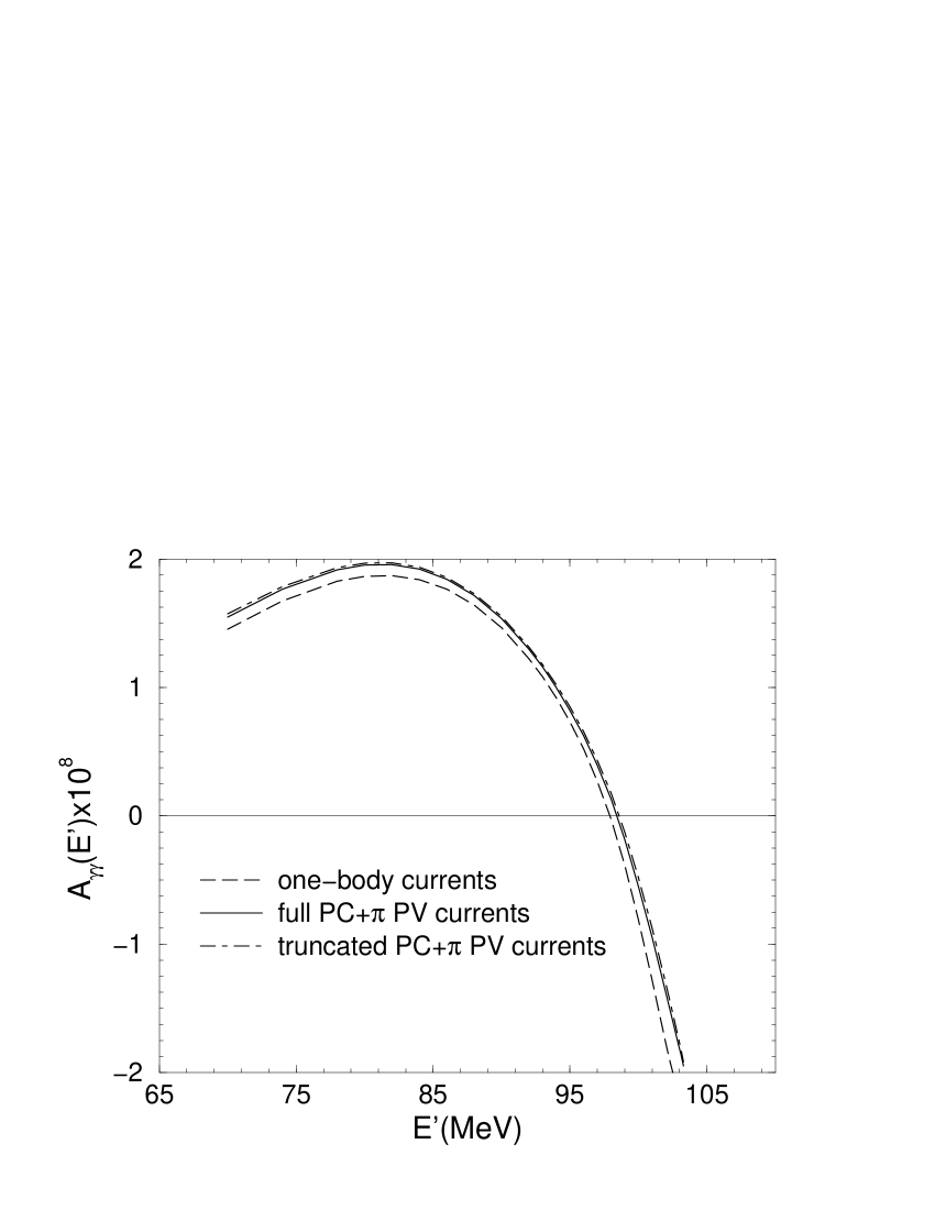
Finally, Fig. 26 is meant to illustrate the sensitivity of the asymmetry to those PC two-body currents derived from the momentum-dependent interaction components of the AV18 model (i.e., the spin-orbit, , and quadratic spin-orbit terms), see Sec. III and VII B. While these currents play a crucial role in the photon asymmetry in the radiative capture at thermal neutron energy, they give negligible contributions to the present observable at quasi-elastic kinematics.
These results demonstrate that, in the kinematics of the SAMPLE experiments [4, 77], the asymmetry from - interference is dominated by one-body currents, and that it is two-orders of magnitude larger than that associated with the PV hadronic weak interaction. Hence even the largest estimates of the weak coupling constant will not affect extractions of single-nucleon matrix elements. These conclusions corroborate those of the authors of Ref. [80], who have carried out a similar study of the impact of hadronic weak interaction on quasi-elastic electro-deuteron scattering.
VIII Conclusions
A systematic study of parity-violating (PV) observables in the system, including the asymmetries in radiative capture and photo-disintegration, the spin rotation and longitudinal asymmetry in elastic scattering, and the asymmetry in electro-disintegration of the deuteron by polarized electrons at quasi-elastic kinematics, has been carried out by using a variety of latest-generation, strong-interaction potentials in combination with the DDH model of the PV hadronic weak interaction. We find that the model dependence of the -capture asymmetry is quite small, at a level similar to the expected contributions of the short-range parts of the interaction. This process is in fact dominated by the long-range interaction components associated with pion exchange. A measurement of the -capture asymmetry is then a clean probe of that physics.
Similarly, we find that the asymmetry in the reaction at quasi-elastic kinematics is a very clean probe of the electro-weak properties of individual nucleons. The processes associated with two nucleons, including PV admixtures in the deuteron and scattering wave functions and electromagnetic two-body currents induced by hadronic weak interactions, play a very small role at the values of momentum transfers explored so far [4, 77].
We also find that the neutron spin rotation is sensitive to both the pion and vector-meson PV couplings to the nucleon, while exhibiting a modest model dependence, at the level of 5-10%, due to the input strong-interaction potential adopted in the calculation. Thus a measurement of this observable [81], when combined with measurements of the asymmetries in radiative capture [2] and elastic scattering [1], could provide useful constraints for some of these PV amplitudes.
The asymmetry in the deuteron disintegration by circularly polarized photons from threshold up to 20 MeV energies is dominated by the short-range components of the DDH interaction. However, it also displays enhanced sensitivity to the short-range behavior in the strong-interaction potentials. Indeed, predictions for the asymmetry at threshold differ by almost a factor of two, depending on whether the Argonne or Bonn 2000 interactions are used in the calculations. Therefore, this observable cannot provide an unambiguous value of short-range weak meson nucleon couplings; however, they would be valuable in placing constraints on the hadronic weak mixing angles.
Finally, the issue of electromagnetic current conservation in the presence of parity-conserving (PC) and PV potetials has been carefully investigated. In particular, in the case of the and processes dramatic cancellations occur betweeen the contributions associated with the two-body currents induced, respectively, by the PC and PV potentials.
Acknowledgments
The authors wish to thank L.E. Marcucci and M. Viviani for interesting discussions and illuminating correspondence, and G. Hale for making available to them experimental data sets of the deuteron photo-disintegration. The work of J.C. and M.P. was supported by the U.S. Department of Energy under contract W-7405-ENG-36, and the work of R.S. was supported by DOE contract DE-AC05-84ER40150 under which the Southeastern Universities Research Association (SURA) operates the Thomas Jefferson National Accelerator Facility. Finally, some of the calculations were made possible by grants of computing time from the National Energy Research Supercomputer Center.
REFERENCES
- [1] A.R. Berdoz et al., Phys. Rev. Lett. 87, 272301 (2001).
- [2] W.M. Snow et al., Nucl. Instrum. and Methods Phys. Res. A 440 729 (2000).
- [3] B. Wojtsekhowski and W.T.H. van Oers (spokespersons), JLAB letter-of-intent 00-002.
- [4] R. Hasty et al., Science 290, 2117 (2000).
- [5] D.T. Spayde et al., Phys. Rev. Lett. 84, 1106 (2000).
- [6] J. Carlson, R. Schiavilla, V.R. Brown, and B.F. Gibson, Phys. Rev. C 65, 035502 (2002).
- [7] R. Schiavilla, J. Carlson, and M. Paris, Phys. Rev. C 67, 032501 (2003).
- [8] B. Desplanques, J.F. Donoghue, and B.R. Holstein, Ann. Phys. (N.Y.) 124, 449 (1980).
- [9] R.B. Wiringa, V.G.J. Stoks, and R. Schiavilla, Phys. Rev. C 51, 38 (1995).
- [10] V.G.J. Stoks, R.A.M. Klomp, C.P.F. Terheggen, and J.J. de Swart, Phys. Rev. C 49, 2950 (1994).
- [11] R. Machleidt, Phys. Rev. C 63, 024001 (2001).
- [12] J.R. Bergervoet et al., Phys. Rev. C 41, 1435 (1990).
- [13] V.G.J. Stoks, R.A.M. Klomp, M.C.M. Rentmeester, and J.J. de Swart, Phys. Rev. C 48, 792 (1993).
- [14] B.v. Przewoski et al., Phys. Rev. C 58, 1897 (1998).
- [15] M. Viviani, R. Schiavilla, and A. Kievsky, Phys. Rev. C 54, 534 (1996).
- [16] R. Schiavilla, V.R. Pandharipande, and D.O. Riska, Phys. Rev. C 41, 309 (1990).
- [17] R. Schiavilla, V.R. Pandharipande, and D.O. Riska, Phys. Rev. C 40, 2294 (1989).
- [18] R. Schiavilla, R.B. Wiringa, V.R. Pandharipande, and J. Carlson, Phys. Rev. C 45, 2628 (1992).
- [19] J. Carlson, D.O. Riska, R. Schiavilla, and R.B. Wiringa, Phys. Rev. C 42, 830 (1990).
- [20] L.E. Marcucci, D.O. Riska, and R. Schiavilla, Phys. Rev. C 58, 3069 (1998).
- [21] R. Schiavilla and D.O. Riska, Phys. Rev. C 43, 437 (1991).
- [22] W.C. Haxton, C.-P. Liu, and M.J. Ramsey-Musolf, Phys. Rev. C 65, 045502 (2002).
- [23] W.C. Haxton, E.M. Henley, and M.J. Musolf, Phys. Rev. Lett. 63, 949 (1989).
- [24] M.J. Musolf and B.R. Holstein, Phys. Rev. D 43, 2956 (1991).
- [25] D.O. Riska, Nucl. Phys. A 678, 79 (2000).
- [26] C.M. Maekawa and U. van Kolck, Phys. Lett. B478, 73 (2000).
- [27] S.L. Zhu, S.J. Puglia, B.R. Holstein, M.J. Ramsey-Musolf, Phys. Rev. D 62, 033008 (2000).
- [28] L.E. Marcucci, R. Schiavilla, M. Viviani, A. Kievsky, S. Rosati, and J.F. Beacom, Phys. Rev. C 63, 015801 (2000).
- [29] L.E. Marcucci, R. Schiavilla, S. Rosati, A. Kievsky, and M. Viviani, Phys. Rev. C 66, 054003 (2002).
- [30] M.J. Musolf, T.W. Donnelly, J. Dubach, S.J. Pollock, S. Kowalski, and E.J. Beise, Phys. Rep. 239, 1 (1994).
- [31] L. Diaconescu, R. Schiavilla, and U. van Kolck, Phys. Rev. C 63, 044007 (2001).
- [32] T.M. Ito et al., in preparation.
- [33] M.L. Goldberger and K.M. Watson, Collision Theory (Wiley, New York, 1964).
- [34] W. Glöckle, The Quantum Mechanical Few-Body Problem (Springer-Verlag, Berlin, 1983).
- [35] J.L. Friar, Ann. Phys. (N.Y.) 104, 380 (1977).
- [36] J.L. Forest, Phys. Rev. C 61, 034007 (2000).
- [37] R. Schiavilla, Nucl. Phys. A 689, 84c (2001).
- [38] E. Fermi, Nuclear Physics (The University of Chicago Press, Chicago, 1950).
- [39] F.C. Michel, Phys. Rev. 133, B329 (1964).
- [40] L. Stodolsky, Phys. Lett. 50B, 352 (1974); Phys. Lett. 96B, 127 (1980).
- [41] Y. Avishai and P. Grange, J. Phys. G 10, L263 (1984).
- [42] A.R. Edmonds, Angular Momentum in Quantum Mechanics (Princeton University Press, Princeton, 1957).
- [43] M. Viviani, A. Kievsky, L.E. Marcucci, S. Rosati, and R. Schiavilla, Phys. Rev. C 61, 064001 (2000).
- [44] K.M. Nollett, R.B. Wiringa, and R. Schiavilla, Phys. Rev. C 63, 024003 (2001).
- [45] M.J. Musolf and T.W. Donnelly, Nucl. Phys. A546, 509 (1992).
- [46] H.J. Pirner and D.O. Riska, Phys. Lett. B44, 151 (1973).
- [47] J.M. Blatt and L.C. Biedenharn, Phys. Rev. 86, 399 (1952).
- [48] H.P. Stapp, T.J. Ypsilantis, and N. Metropolis, Phys. Rev. 105, 302 (1957).
- [49] M. Lacombe, B. Loiseau, J.-M. Richard, R. Vinh Mau, P. Pireraud, and R. de Toureil, Phys. Rev. C 21, 861 (1980).
- [50] D. Bowman, private communication.
- [51] A.E. Cox, S.A.R. Wynchank, and C.H. Collie, Nucl. Phys. 74, 497 (1965).
- [52] S.F. Mughabghab, M. Divadeenam, and N.E. Holden, Neutron Cross Sections from Neutron Resonance Parameters and Thermal Cross Sections (Academic Press, London, 1981), http://isotopes.lbl.gov/ngdata/sig.htm.
- [53] B. Desplanques, Nucl. Phys. A242, 423 (1975); ibidem A335, 147 (1980).
- [54] B.H.J. McKellar, Nucl. Phys. A254, 147 (1975).
- [55] B. Desplanques, Phys. Lett. B512, 305 (2001).
- [56] C.H. Hyun, T.-S. Park, and D.-P. Min, Phys. Lett. B516, 321 (2001).
- [57] R.B. Wiringa and S.C. Pieper, Phys. Rev. Lett. 89, 182501 (2002).
- [58] L.E. Marcucci, A. Kievsky, S. Rosati, R. Schiavilla, and M. Viviani, private communication.
- [59] G.R. Bishop et al., Phys. Rev. 80, 211 (1950).
- [60] A.H. Snell, E.C. Barker, and R.L. Sternberg, Phys. Rev. 80, 637 (1950).
- [61] S.A. Colgate, Phys. Rev. 83, 1262 (1951).
- [62] J.H. Carver et al., Nature 167, 154 (1951).
- [63] Y. Birenbaum, S. Kahane, and R. Moreh, Phys. Rev. C 32, 1825 (1985).
- [64] R. Moreh, T.J. Kennett, and W.V. Prestwich, Phys. Rev. C 39, 1247 (1989).
- [65] A. De Graeve et al., Phys. Rev. C 45, 860 (1992).
- [66] G.S. Danilov, Phys. Lett. 18, 40 (1965).
- [67] J.L. Friar and B.H.J. McKellar, Phys. Lett. 123B, 284 (1983).
- [68] E. Hadjimichael and E. Fischbach, Phys. Rev. D 3, 755 (1971).
- [69] K.R. Lassey and B.H.J. McKellar, Phys. Rev. C 11, 349 (1975) and 12, 721 (E) (1975).
- [70] B.A. Craver, E. Fischbach, Y.E. Kim, and A. Tubis, Phys. Rev. D 13, 1376 (1976).
- [71] H.C. Lee, Phys. Rev. Lett. 41, 843 (1978).
- [72] E.M. Henley, Ann. Rev. Nucl. Sci. 19, 367 (1969).
- [73] T. Oka, Phys. Rev. D 27, 523 (1983).
- [74] T. Hamada and I.D. Johnston, Nucl. Phys. 34, 382 (1962).
- [75] V.A. Knyaz’kov et al., Nucl. Phys. A417, 209 (1984).
- [76] V.M. Lobashov et al., Nucl. Phys. A197, 241 (1972).
- [77] D.H. Beck and R.D. McKeown, Ann. Rev. Nucl. Part. Sci. 51, 189 (2001).
- [78] W.-Y. P. Hwang and E.M. Henley, Ann. Phys. (N.Y.) 129, 47 (1980).
- [79] W.-Y. P. Hwang, E.M. Henley, and G.A. Miller, Ann. Phys. (N.Y.) 137, 378 (1981).
- [80] C.-P. Liu, G. Prezeau, and M.J. Ramsey-Musolf, Phys. Rev. C 67, 035502 (2003).
- [81] W.M. Snow, private communication.
| 1 | 2 | 3 | 4 | |
|---|---|---|---|---|
| 0 | 1S0 | 3P0 | ||
| 1 | 3S1 | 3D1 | 1P1 | 3P1 |
| 2 | 3P2 | 3F2 | 1D2 | 3D2 |
| 3 | 3D3 | 3G3 | 1F3 | 3F3 |
| coupling | |||||
|---|---|---|---|---|---|
| 12 | 13 | 14 | 23 | 24 | |
| 0 | PV | ||||
| 1 | PC | PV | PV | PV | PV |
| 2 | PC | PV | PV | PV | PV |
| PC | PV | PV | PV | PV | |
| AV18 | |||
|---|---|---|---|
| NIJM-I | |||
| BONN | |||
| Plane waves |
| (mb) | ||||
|---|---|---|---|---|
| Interaction | ||||
| AV18 | ||||
| NIJM-I | ||||
| BONN | ||||
| Impulse | ||
|---|---|---|
| -dependent |
| (mb) | ||||
|---|---|---|---|---|
| Impulse | ||||
| Siegert | ||||
| Impulse | |||
|---|---|---|---|
| Full |