Abstract

We perform a study of infinite hadronic matter, finite nuclei and hypernuclei with an improved method of calculating the effective baryon mass. A detailed study of the predictions of the model is made in comparison with the available data and the level of agreement is generally very good. Comparison with an earlier treatment shows relatively minor differences at or below normal nuclear matter density, while at high density the improved calculation is quite different. In particular, we find no phase transition corresponding to chiral symmetry restoration in high density nuclear matter.

PACS number(s): 21.65.+f; 21.10-k; 21.80+a; 12.39.-x

Keywords: Hadronic Matter, Finite Nuclei, Hypernuclei, Effective Mass,

Chiral Symmetry, Quark Mean Field

I Introduction

The complex action of QCD at finite chemical potential makes it difficult to study finite-density QCD properties directly from first principle lattice calculations. There are many phenomenological models based on hadron degrees of freedom, such as the Walecka model [1], the Zimanyi-Mozkovski model [2] and the nonlinear $\sigma-\omega$ model [3], as well as models which explicitly include quark degrees of freedom, for example, the quark meson coupling model [4], the cloudy bag model [5], the quark mean field model [6] and the NJL model [7]. With the development of these phenomenological models, the interactions between hadrons become more and more complex. The symmetries of QCD can be used to determine largely how the hadrons should interact with each other. With this in mind, the chiral $SU(2)$ $\times$ $SU(2)$ effective quark model was proposed. It has been used widely to investigate nuclear matter and finite nuclei at both zero and finite temperature [8]-[15].

In the last twenty years, exploring systems with strangeness, especially with a large strangeness fraction, has attracted a lot of interest. Therefore, a model which includes strange quarks or hyperons is needed. Papazoglou $et$ $al$. [16, 17] proposed a chiral $SU(3)$ model which extended the $SU(2)$ chiral symmetry to $SU(3)$$\times$$SU(3)$. Recently, a chiral $SU(3)$ quark mean field model based on quark degrees of freedom was proposed by Wang $et$ $al$. [18, 19]. In this model, quarks are confined in the baryons by an effective potential. The quark-meson interaction and meson self-interaction are based on $SU(3)$ chiral symmetry. Through the mechanism of spontaneous symmetry breaking the resulting constituent quarks and mesons (except for the pseudoscalars) obtain masses. The introduction of an explicit symmetry breaking term in the meson self-interaction generates the masses of the pseudoscalar mesons which satisfy the relevant PCAC relations. The explicit symmetry breaking term in the quark-meson interaction gives reasonable hyperon potentials in hadronic matter. This chiral $SU(3)$ quark mean field model has been applied to investigate nuclear matter [20], strange hadronic matter [18], finite nuclei, hypernuclei [19], and quark matter [21]. By and large the results are in reasonable agreement with existing experimental data.

A surprising result, which is quite different from most other models is that at some critical density the effective baryon mass drops to zero [22]. There is a first order phase transition around this critical density where the physical quantities change discontinuously. We will see later that this behavior is primarily a consequence of the nonlinear ansatz for the effective baryon mass which is related to the subtraction of the centre of mass (c.m.) motion. In Ref. [23], the authors provided an exact solution of the effect of c.m. motion and found that it was only very weakly dependent on the external field strength for the densities of interest. As a result, the c.m. correction can be included in the zero point energy. In this paper, we will use this alternative definition of the effective baryon mass in medium to reexamine the properties of hadronic matter.

The paper is organized as follows. The model is introduced in section II. In section III, we study infinite hadronic matter, finite nuclei, and hypernuclei with the improved treatment of the centre of mass correction to the baryon mass in medium. The numerical results are presented in section IV and section V is the summary.

II The model

Our considerations are based on the chiral $SU(3)$ quark mean field model (for details see Refs. [18, 19]), which contains quarks and mesons as basic degrees of freedom. In the chiral limit, the quark field $q$ can be split into left and right-handed parts $q_{L}$ and $q_{R}$: $q\,=\,q_{L}\,+\,q_{R}$. Under $SU(3)$${}_{L}\times$ $SU(3)$_R they transform as

$$q_{L}\rightarrow q_{L}^{\prime}\,=\,L\,q_{L},~{}~{}~{}~{}~{}q_{R}\rightarrow q_{R}^{\prime}\,=\,R\,q_{R}\,.$$ (1)

The spin-0 mesons are written in the compact form

$$M(M^{+})=\Sigma\pm i\Pi=\frac{1}{\sqrt{2}}\sum_{a=0}^{8}\left(s^{a}\pm ip^{a}\right)\lambda^{a},$$ (2)

where $s^{a}$ and $p^{a}$ are the nonets of scalar and pseudoscalar mesons, respectively, $\lambda^{a}(a=1,...,8)$ are the Gell-Mann matrices, and $\lambda^{0}=\sqrt{\frac{2}{3}}\,I$. The alternatives, plus and minus signs correspond to $M$ and $M^{+}$. Under chiral $SU(3)$ transformations, $M$ and $M^{+}$ transform as $M\rightarrow M^{\prime}=LMR^{+}$ and $M^{+}\rightarrow M^{+^{\prime}}=RM^{+}L^{+}$. The spin-1 mesons are arranged in a similar way as

$$l_{\mu}(r_{\mu})=\frac{1}{2}\left(V_{\mu}\pm A_{\mu}\right)=\frac{1}{2\sqrt{2}}\sum_{a=0}^{8}\left(v_{\mu}^{a}\pm a_{\mu}^{a}\right)\lambda^{a}$$ (3)

with the transformation properties: $l_{\mu}\rightarrow l_{\mu}^{\prime}=Ll_{\mu}L^{+}$, $r_{\mu}\rightarrow r_{\mu}^{\prime}=Rr_{\mu}R^{+}$. The matrices $\Sigma$, $\Pi$, $V_{\mu}$ and $A_{\mu}$ can be written in a form where the physical states are explicit. For the scalar and vector nonets, we have the expressions

$$\Sigma=\frac{1}{\sqrt{2}}\sum_{a=0}^{8}s^{a}\,\lambda^{a}=\left(\begin{array}[]{lcr}\frac{1}{\sqrt{2}}\left(\sigma+a_{0}^{0}\right)&a_{0}^{+}&K^{*+}\\ a_{0}^{-}&\frac{1}{\sqrt{2}}\left(\sigma-a_{0}^{0}\right)&K^{*0}\\ K^{*-}&\bar{K}^{*0}&\zeta\end{array}\right),$$ (7)

$$V_{\mu}=\frac{1}{\sqrt{2}}\sum_{a=0}^{8}v_{\mu}^{a}\,\lambda^{a}=\left(\begin{array}[]{lcr}\frac{1}{\sqrt{2}}\left(\omega_{\mu}+\rho_{\mu}^{0}\right)&\rho_{\mu}^{+}&K_{\mu}^{*+}\\ \rho_{\mu}^{-}&\frac{1}{\sqrt{2}}\left(\omega_{\mu}-\rho_{\mu}^{0}\right)&K_{\mu}^{*0}\\ K_{\mu}^{*-}&\bar{K}_{\mu}^{*0}&\phi_{\mu}\end{array}\right).$$ (11)

Pseudoscalar and pseudovector nonet mesons can be written in a similar fashion.

The total effective Lagrangian is written:

$${\cal L}_{{\rm eff}}\,=\,{\cal L}_{q0}\,+\,{\cal L}_{qM}\,+\,{\cal L}_{\Sigma\Sigma}\,+\,{\cal L}_{VV}\,+\,{\cal L}_{\chi SB}\,+\,{\cal L}_{\Delta m_{s}}\,+\,{\cal L}_{h},+\,{\cal L}_{c},$$ (12)

where ${\cal L}_{q0}=\bar{q}\,i\gamma^{\mu}\partial_{\mu}\,q$ is the free part for massless quarks. The quark-meson interaction ${\cal L}_{qM}$ can be written in a chiral $SU(3)$ invariant way as

$${\cal L}_{qM}=g_{s}\left(\bar{\Psi}_{L}M\Psi_{R}+\bar{\Psi}_{R}M^{+}\Psi_{L}\right)-g_{v}\left(\bar{\Psi}_{L}\gamma^{\mu}l_{\mu}\Psi_{L}+\bar{\Psi}_{R}\gamma^{\mu}r_{\mu}\Psi_{R}\right)~{}~{}~{}~{}~{}~{}~{}~{}~{}~{}~{}~{}~{}~{}~{}~{}~{}~{}~{}~{}~{}~{}~{}$$ (13)

$$=\frac{g_{s}}{\sqrt{2}}\bar{\Psi}\left(\sum_{a=0}^{8}s_{a}\lambda_{a}+i\gamma^{5}\sum_{a=0}^{8}p_{a}\lambda_{a}\right)\Psi-\frac{g_{v}}{2\sqrt{2}}\bar{\Psi}\left(\gamma^{\mu}\sum_{a=0}^{8}v_{\mu}^{a}\lambda_{a}-\gamma^{\mu}\gamma^{5}\sum_{a=0}^{8}a_{\mu}^{a}\lambda_{a}\right)\Psi.$$ (14)

In the mean field approximation, the chiral-invariant scalar meson ${\cal L}_{\Sigma\Sigma}$ and vector meson ${\cal L}_{VV}$ self-interaction terms are written as [18, 19]

$${\cal L}_{\Sigma\Sigma} = -\frac{1}{2}\,k_{0}\chi^{2}\left(\sigma^{2}+\zeta^{2}\right)+k_{1}\left(\sigma^{2}+\zeta^{2}\right)^{2}+k_{2}\left(\frac{\sigma^{4}}{2}+\zeta^{4}\right)+k_{3}\chi\sigma^{2}\zeta$$ (16)

$$-k_{4}\chi^{4}-\frac{1}{4}\chi^{4}\ln\frac{\chi^{4}}{\chi_{0}^{4}}+\frac{\delta}{3}\chi^{4}\ln\frac{\sigma^{2}\zeta}{\sigma_{0}^{2}\zeta_{0}},$$

$${\cal L}_{VV} = \frac{1}{2}\,\frac{\chi^{2}}{\chi_{0}^{2}}\left(m_{\omega}^{2}\omega^{2}+m_{\rho}^{2}\rho^{2}+m_{\phi}^{2}\phi^{2}\right)+g_{4}\left(\omega^{4}+6\omega^{2}\rho^{2}+\rho^{4}+2\phi^{4}\right),$$ (17)

where $\delta=6/33$; $\sigma_{0}$, $\zeta_{0}$ and $\chi_{0}$ are the vacuum expectation values of the corresponding mean fields $\sigma$, $\zeta$ and $\chi$.

From the quark-meson interaction, the coupling constants between scalar mesons, vector mesons and quarks have the following relations:

$$\frac{g_{s}}{\sqrt{2}} = g_{a_{0}}^{u}=-g_{a_{0}}^{d}=g_{\sigma}^{u}=g_{\sigma}^{d}=\ldots=\frac{1}{\sqrt{2}}g_{\zeta}^{s},~{}~{}~{}~{}~{}g_{a_{0}}^{s}=g_{\sigma}^{s}=g_{\zeta}^{u}=g_{\zeta}^{d}=0\,,$$ (18)

$$\frac{g_{v}}{2\sqrt{2}} = g_{\rho^{0}}^{u}=-g_{\rho^{0}}^{d}=g_{\omega}^{u}=g_{\omega}^{d}=\ldots=\frac{1}{\sqrt{2}}g_{\phi}^{s},~{}~{}~{}~{}~{}g_{\omega}^{s}=g_{\rho^{0}}^{s}=g_{\phi}^{u}=g_{\phi}^{d}=0.$$ (19)

Note, the values of $\sigma_{0}$, $\zeta_{0}$ and $\chi_{0}$ are determined from a minimization of the thermodynamic potential. On the other hand, the parameters $\sigma_{0}$ and $\zeta_{0}$ are constrained by the spontaneous breaking of chiral symmetry and are expressed by the pion ($F_{\pi}$ = 93 MeV) and the kaon ($F_{K}$ = 115 MeV) leptonic decay constants as:

$$\sigma_{0}=-F_{\pi}\hskip 28.45274pt\hskip 28.45274pt\zeta_{0}=\frac{1}{\sqrt{2}}(F_{\pi}-2F_{K})$$ (20)

The Lagrangian ${\cal L}_{\chi SB}$ generates the nonvanishing masses of pseudoscalar mesons

$${\cal L}_{\chi SB}=\frac{\chi^{2}}{\chi_{0}^{2}}\left[m_{\pi}^{2}F_{\pi}\sigma+\left(\sqrt{2}\,m_{K}^{2}F_{K}-\frac{m_{\pi}^{2}}{\sqrt{2}}F_{\pi}\right)\zeta\right],$$ (21)

leading to a nonvanishing divergence of the axial currents which in turn satisfy the partial conserved axial-vector current (PCAC) relations for $\pi$ and $K$ mesons. Pseudoscalar, scalar mesons and also the dilaton field $\chi$ obtain mass terms by spontaneous breaking of chiral symmetry in the Lagrangian (16). The masses of $u$, $d$ and $s$ quarks are generated by the vacuum expectation values of the two scalar mesons $\sigma$ and $\zeta$. To obtain the correct constituent mass of the strange quark, an additional mass term has to be added:

$${\cal L}_{\Delta m_{s}}=-\Delta m_{s}\bar{q}Sq$$ (22)

where $S\,=\,\frac{1}{3}\,\left(I-\lambda_{8}\sqrt{3}\right)={\rm diag}(0,0,1)$ is the strangeness quark matrix. Based on these mechanisms, the quark constituent masses are finally given by

$$m_{u}=m_{d}=-\frac{g_{s}}{\sqrt{2}}\sigma_{0}\hskip 14.22636pt\mbox{and}\hskip 14.22636ptm_{s}=-g_{s}\zeta_{0}+\Delta m_{s}.$$ (23)

The parameters $g_{s}=4.76$ and $\Delta m_{s}=29$ MeV are chosen to yield the constituent quark masses $m_{q}=313$ MeV and $m_{s}=490$ MeV. In order to obtain reasonable hyperon potentials in hadronic matter, we include an additional coupling between strange quarks and the scalar mesons $\sigma$ and $\zeta$ [18]. This term is expressed as

$${\cal L}_{h}\,=\,(h_{1}\,\sigma\,+\,h_{2}\,\zeta)\,\bar{s}s\,.$$ (24)

In the quark mean field model, quarks are confined in baryons by the Lagrangian ${\cal L}_{c}=-\bar{\Psi}\,\chi_{c}\,\Psi$ (with $\chi_{c}$ given in Eq. (25), below). The Dirac equation for a quark field $\Psi_{ij}$ under the additional influence of the meson mean fields is given by

$$\left[-i\vec{\alpha}\cdot\vec{\nabla}+\chi_{c}(r)+\beta m_{i}^{*}\right]\Psi_{ij}=e_{i}^{*}\Psi_{ij},$$ (25)

where $\vec{\alpha}=\gamma^{0}\vec{\gamma}$ , $\beta=\gamma^{0}$ , the subscripts $i$ and $j$ denote the quark $i$ ($i=u,d,s$) in a baryon of type $j$ ($j=N,\Lambda,\Sigma,\Xi$) ; $\chi_{c}(r)$ is a confinement potential, i.e. a static potential providing confinement of quarks by meson mean-field configurations. The quark mass $m_{i}^{*}$ and energy $e_{i}^{*}$ are defined as

$$m_{i}^{*}=-g_{\sigma}^{i}\sigma-g_{\zeta}^{i}\zeta+m_{i0}$$ (26)

and

$$e_{i}^{*}=e_{i}-g_{\omega}^{i}\omega-g_{\phi}^{i}\phi\,,$$ (27)

where $e_{i}$ is the energy of the quark under the influence of the meson mean fields. Here $m_{i0}=0$ for $i=u,d$ (nonstrange quark) and $m_{i0}=\Delta m_{s}=29$ MeV for $i=s$ (strange quark). Using the solution of the Dirac equation (25) for the quark energy $e_{i}^{*}$ it has been common to define the effective mass of the baryon $j$ through the ansatz:

$$M_{j}^{*}=\sqrt{E_{j}^{*2}-<p_{j\,cm}^{*2}>}\,,$$ (28)

where $E_{j}^{*}=\sum_{i}n_{ij}e_{i}^{*}+E_{j\,spin}$ is the baryon energy and $<p_{j\,cm}^{*2}>$ is the subtraction of the contribution to the total energy associated with spurious center of mass motion. In the expression for the baryon energy $n_{ij}$ is the number of quarks with flavor $"i"$ in a baryon with flavor $j$, with $j=N\,\{p,n\}\,,\Sigma\,\{\Sigma^{\pm},\Sigma^{0}\}\,,\Xi\,\{\Xi^{0},\Xi^{-}\}\,,\Lambda\,$ and $E_{j\,spin}$ is the correction to the baryon energy which is determined from a fit to the data for baryon masses.

There is an alternative way to remove the spurious c.m. motion and determine the effective baryon masses. In Ref. [23], the removal of the spurious c.m. motion for three quarks moving in a confining, relativistic oscillator potential was studied in some detail. It was found that when an external scalar potential was applied, the effective mass obtained from the interaction Lagrangian could be written as

$$M_{j}^{*}=\sum_{i}n_{ij}e_{i}^{*}-E_{j}^{0}\,,$$ (29)

where $E_{j}^{0}$ was found to be only very weakly dependent on the external field strength. We therefore use Eq. (29), with $E_{j}^{0}$ a constant, independent of the density, which is adjusted to give a best fit to the free baryon masses.

Using the square root ansatz for the effective baryon mass, Eq. (28), the confining potential $\chi_{c}$ is chosen as a combination of scalar (S) and scalar-vector (SV) potentials as in Ref. [19]:

$$\chi_{c}(r)=\frac{1}{2}[\,\chi_{c}^{\rm S}(r)+\chi_{c}^{\rm SV}(r)\,]$$ (30)

with

$$\chi_{c}^{\rm S}(r)=\frac{1}{4}k_{c}\,r^{2}\,,$$ (31)

and

$$\chi_{c}^{\rm SV}(r)=\frac{1}{4}k_{c}\,r^{2}(1+\gamma^{0})\,.$$ (32)

On the other hand, using the linear definition of effective baryon mass, Eq. (29), the confining potential $\chi_{c}$ is chosen to be the purely scalar potential $\chi_{c}^{\rm S}(r)$. The coupling $k_{c}$ is taken as $k_{c}=1$ (GeV fm${}^{-2})$, which yields baryon radii of about 0.6 fm. In both cases, the baryon masses in vacuum are chosen as: $M_{N}=939$ MeV, $M_{\Lambda}=1116$ MeV, $M_{\Sigma}=1196$ MeV and $M_{\Xi}=1318$ MeV.

III hadronic system

Based on the previously defined quark mean field model the effective Lagrangian for the study of hadronic systems is written as

$${\cal L}_{H} = \bar{\psi}_{B}(i\gamma^{\mu}\partial_{\mu}-M_{B}^{*})\psi_{B}+\frac{1}{2}\partial_{\mu}\sigma\partial^{\mu}\sigma+\frac{1}{2}\partial_{\mu}\zeta\partial^{\mu}\zeta+\frac{1}{2}\partial_{\mu}\chi\partial^{\mu}\chi-\frac{1}{4}F_{\mu\nu}F^{\mu\nu}-\frac{1}{4}S_{\mu\nu}S^{\mu\nu}$$ (35)

$$-\frac{1}{4}E_{\mu\nu}E^{\mu\nu}-g_{\omega}^{B}\bar{\psi}_{B}\gamma_{\mu}\psi_{B}\omega^{\mu}-g_{\phi}^{B}\bar{\psi}_{B}\gamma_{\mu}\psi_{B}\phi^{\mu}-\frac{1}{2}g_{\rho}^{B}\bar{\psi}_{B}\gamma_{\mu}\psi_{B}\rho^{\mu}$$

$$-e_{B}\bar{\psi}_{B}\gamma_{\mu}\psi_{B}A^{\mu}+{\cal L}_{M},$$

where

$$F_{\mu\nu}=\partial_{\mu}\omega_{\nu}-\partial_{\nu}\omega_{\mu},$$ (36)

$$S_{\mu\nu}=\partial_{\mu}\phi_{\nu}-\partial_{\nu}\phi_{\mu},$$ (37)

$$E_{\mu\nu}=\partial_{\mu}A_{\nu}-\partial_{\nu}A_{\mu}.$$ (38)

$e_{B}$ is the coupling constant of comloub interaction. The mesonic Lagrangian

$${\cal L}_{M}={\cal L}_{\Sigma\Sigma}+{\cal L}_{VV}+{\cal L}_{\chi SB}$$ (39)

describes the interaction between mesons which includes the scalar meson self-interaction ${\cal L}_{\Sigma\Sigma}$, the vector meson self-interaction ${\cal L}_{VV}$ and the explicit chiral symmetry breaking term ${\cal L}_{\chi SB}$ defined previously in Eqs. (16), (17) and (21). The Lagrangian ${\cal L}_{M}$ involves scalar ($\sigma$, $\zeta$ and $\chi$) and vector ($\omega$ and $\phi$) mesons. The interactions between quarks and scalar mesons result in the effective baryon masses $M_{B}^{*}$, where subscript $B$ labels the baryon flavor $B=N,\Lambda,\Sigma$ or $\Xi$. The interactions between quarks and vector mesons generate the baryon-vector meson interaction terms. The corresponding vector coupling constants $g_{\omega}^{B}$ and $g_{\phi}^{B}$ satisfy the $SU(3)$ flavor symmetry relations:

$$g_{\omega}^{\Lambda}=g_{\omega}^{\Sigma}=2g_{\omega}^{\Xi}=\frac{2}{3}g_{\omega}^{N}=2g_{\omega}^{u}=\frac{g_{v}}{\sqrt{2}}\hskip 14.22636pt\mbox{and}\hskip 14.22636ptg_{\phi}^{\Lambda}=g_{\phi}^{\Sigma}=\frac{1}{2}g_{\phi}^{\Xi}=\frac{\sqrt{2}}{3}g_{\omega}^{N}=g_{\phi}^{s}=\frac{g_{v}}{2}.$$ (40)

Compared with the chiral $SU(3)$ model of Refs. [16] and [17], the mesonic Lagrangian is the same. However, that model is based on the hadron degree of freedom and the effective baryon masses are obtained from the direct baryon-meson coupling. This chiral $SU(3)$ quark mean field model is on the quark level and the effective baryon masses are generated by quarks which couple with mesons and are confined in baryons by a potential. In the earlier work, the effective baryon masses are calculated with the square root ansatz. In this paper, we use the improved linear definition of baryon masses.

The equations for mesons $\phi_{i}$ can be obtained by the formula $-\frac{\partial{\cal L}_{H}}{\partial^{\mu}(\partial_{\mu}\phi)}-\frac{\partial{\cal L}_{H}}{\partial\phi}=0$. Therefore, the equations for $\sigma$, $\zeta$ and $\chi$ are

$$-\partial_{\mu}\partial^{\mu}\sigma+k_{0}\chi^{2}\sigma-4k_{1}\left(\sigma^{2}+\zeta^{2}\right)\sigma-2k_{2}\sigma^{3}-2k_{3}\chi\sigma\zeta-\frac{2\delta}{3\sigma}\chi^{4}+\frac{\chi^{2}}{\chi_{0}^{2}}m_{\pi}^{2}F_{\pi}$$ (41)

$$-\left(\frac{\chi}{\chi_{0}}\right)^{2}m_{\omega}\omega^{2}\frac{\partial m_{\omega}}{\partial\sigma}+\sum_{B=N\,,\Lambda\,,\Sigma\,,\Xi}\frac{\partial M_{B}^{\ast}}{\partial\sigma}<\bar{\psi_{B}}\psi_{B}>=0,~{}~{}~{}~{}~{}~{}~{}~{}~{}~{}$$ (42)

$$-\partial_{\mu}\partial^{\mu}\zeta+k_{0}\chi^{2}\zeta-4k_{1}\left(\sigma^{2}+\zeta^{2}\right)\zeta-4k_{2}\zeta^{3}-k_{3}\chi\sigma^{2}-\frac{\delta}{3\zeta}\chi^{4}+\frac{\chi^{2}}{\chi_{0}^{2}}\left(\sqrt{2}m_{k}^{2}F_{k}-\frac{1}{\sqrt{2}}m_{\pi}^{2}F_{\pi}\right)$$ (43)

$$-\left(\frac{\chi}{\chi_{0}}\right)^{2}m_{\phi}\phi^{2}\frac{\partial m_{\phi}}{\partial\zeta}+\sum_{B=\Lambda\,,\Sigma\,,\Xi}\frac{\partial M_{B}^{\ast}}{\partial\zeta}<\bar{\psi_{B}}\psi_{B}>=0,~{}~{}~{}~{}~{}~{}~{}~{}~{}~{}~{}~{}~{}~{}~{}~{}~{}~{}~{}~{}~{}~{}~{}$$ (44)

$$-\partial_{\mu}\partial^{\mu}\chi+k_{0}\chi\left(\sigma^{2}+\zeta^{2}\right)-k_{3}\sigma^{2}\zeta+\left(4k_{4}+1+4\ln\frac{\chi}{\chi_{0}}-\frac{4\delta}{3}\ln\frac{\sigma^{2}\zeta}{\sigma_{0}^{2}\zeta_{0}}\right)\chi^{3}$$ (45)

$$+\frac{2\chi}{\chi_{0}^{2}}\left[m_{\pi}^{2}F_{\pi}\sigma+\left(\sqrt{2}m_{k}^{2}F_{k}-\frac{1}{\sqrt{2}}m_{\pi}^{2}F_{\pi}\right)\zeta\right]-\frac{\chi}{\chi_{0}^{2}}m_{\omega}^{2}\omega^{2}=0.$$ (46)

For infinite hadronic matter, the meson mean field is independent of position and $<\bar{\psi}_{B}\psi_{B}>$ is expressed as

$$<\bar{\psi}_{B}\psi_{B}> = \frac{g_{B}\,M_{B}^{\ast}}{\pi^{2}}\,\int_{0}^{k_{F_{B}}}dk\frac{k^{2}}{\sqrt{M_{B}^{\ast 2}+k^{2}}}$$ (47)

$$= \frac{g_{B}\,M_{B}^{\ast 3}}{2\,\pi^{2}}\,\biggl{[}\frac{k_{F_{B}}}{M_{B}^{\ast}}\,\sqrt{1+\frac{k_{F_{B}}^{2}}{M_{B}^{\ast 2}}}-\ln\biggl{(}\frac{k_{F_{B}}}{M_{B}^{\ast}}+\sqrt{1+\frac{k_{F_{B}}^{2}}{M_{B}^{\ast 2}}}\biggr{)}\biggr{]}.$$ (48)

For finite nuclei, the integration in $<\bar{\psi_{B}}\psi_{B}>$ will change to a sum over the states $\psi_{B}^{\alpha}$, which are obtained from the Dirac equation for the baryon $B$ in state $\alpha$

$$\left[-i\gamma\cdot\vec{\nabla}+M_{B}^{*}+g_{\omega}^{B}\omega\gamma_{0}+g_{\phi}^{B}\phi\gamma_{0}+\frac{1}{2}g_{\rho}^{B}\rho\gamma_{0}+e_{B}A_{0}\gamma_{0}\right]\psi_{\alpha}^{B}=\epsilon_{\alpha}\gamma_{0}\psi_{\alpha}^{B}.$$ (49)

This set of coupled equations is solved iteratively. At each iteration, we first solve the equations for the quark wave function using fourth-order Runge-Kutta for given meson fields and obtain the effective baryon masses. We then solve the equations for the nucleon radial wave functions with the same method. The corresponding scalar and vector densities can be obtained. Then the mean meson fields which will be used in the next iteration step are determined for the calculated densities. The iteration is stopped when convergence is achieved. The energy for the finite system within the mean field approximation can be derived in the standard way.

$$E=\sum_{j=N,\Lambda,\Xi;\alpha=1}^{\Omega}\epsilon_{\alpha}^{j}(2j_{\alpha}+1)-\frac{1}{2}\int d^{3}r((\sigma\frac{\partial M_{j}^{*}}{\partial\sigma}+\zeta\frac{\partial M_{j}^{*}}{\partial\zeta})\rho_{s}^{j}+g_{\omega}^{j}\omega\rho_{v}^{j}+g_{\phi}^{j}\phi\rho_{v}^{j}+g_{\rho}^{j}\rho\rho_{v}^{j})+E_{rearr},$$ (50)

where $\rho_{s}^{j}=\bar{\psi}_{j}\psi_{j}$ and $\rho_{v}^{j}=\bar{\psi}_{j}\gamma_{0}\psi_{j}$. $\epsilon_{\alpha}^{j}$ are the Dirac single particle energies and $j_{\alpha}$ are the total angular momenta of the single particle states. By using the equations of meson fields, the rearrangement energy $E_{rearr}$ can be written as

$$E_{rearr} = \int d^{3}r\left\{g_{4}(\omega^{4}+\rho^{4}+6\omega^{2}\rho^{2}+2\phi^{4})-k_{1}(\sigma^{2}+\zeta^{2})^{2}-k_{2}\left(\frac{\sigma^{4}}{2}+\zeta^{4}\right)\right.$$ (53)

$$\left.-\frac{1}{2}k_{3}\chi\sigma^{3}\zeta+\frac{\delta}{3}\chi^{4}\ln\left(\frac{\sigma^{2}\zeta}{\sigma_{0}^{2}\zeta_{0}^{2}}\right)+\frac{1}{2}\frac{\chi^{2}}{\chi_{0}^{2}}m_{\pi}^{2}f_{\pi}\sigma\right.$$

$$\left.+\frac{1}{2}\frac{\chi^{2}}{\chi_{0}^{2}}\left(\sqrt{2}m_{K}^{2}f_{K}-\frac{1}{\sqrt{2}}m_{\pi}^{2}f_{\pi}\right)\zeta\right\}-V_{vac},$$

where the constant $V_{vac}$ is the vacuum energy which is subtracted to yield zero energy in the vacuum.

IV numerical results

Before doing detailed numerical studies, we first determine the parameters in the model. The coupling constant $g_{s}$ as well as $\Delta m_{s0}$ are determined by the constituent quark masses, $m_{q}$ and $m_{s}$. $m_{v}$ and $\mu$ are obtained by fitting the vector meson masses. The confining coefficient, $k_{c}$, is chosen to be 1000 MeVfm^-2 to make the baryon radii (in the absence of a pion cloud [24]) around 0.6 fm. For nuclear matter, there are seven other parameters, $k_{0}$, $k_{1}$, $k_{2}$, $k_{3}$, $k_{4}$, $g_{4}$ and $g_{v}$, to be determined. We fit them to the $\pi$-meson mass, $K$-meson mass and the average mass of $\eta$ and $\eta^{\prime}$ which are given by the eigenvalues of the mass matrix

$$M_{ij}=-\frac{\delta^{2}{\cal L}_{H}}{\delta\phi_{i}\delta\phi_{j}}.$$ (54)

There are two constraints associated with the saturation properties of nuclear matter. We choose the parameters to fit the binding energy of nuclear matter $\varepsilon/\rho-M_{N}=-16$ MeV at saturation density $\rho_{0}=0.16$ fm^-3. The parameters should also produce a reasonable compression modulus and effective nucleon mass at saturation density. For strange matter, there are two additional parameters $h_{1}$ and $h_{2}$ to be determined. They are restricted by the hyperon potentials in hadronic matter. All these nine parameters are listed in Table I with the two methods for computing the effective baryon mass. The properties of nuclear matter and the masses of $\sigma$ and $\zeta$ are listed in the Table II. From the table, one can see that the main difference between the two versions is that in the linear definition (Eq. (29)), the effective mass is larger. In fact, if we choose a larger value of $g_{4}$, the effective mass will be smaller. However, in that case the results for finite nuclei will not be so good.

TABLE I.: Parameters of the model.

version	$k_{0}$	$k_{1}$	$k_{2}$	$k_{3}$	$k_{4}$	$g_{s}$	$g_{v}$	$g_{4}$	$h_{1}$	$h_{2}$
square	4.21	2.26	-10.16	-4.38	-0.13	4.76	10.99	7.5	-2.07	2.90
linear	3.97	2.18	-10.16	-4.15	-0.14	4.76	8.70	15.0	-2.66	2.45

TABLE II.: Nuclear properties and scalar meson masses.

version	$\rho_{0}$ (fm-3)	E/A (MeV)	$M^{*}_{N}/M_{N}$	K (MeV)	$m_{\sigma}$ (MeV)	$m_{\zeta}$ (MeV)
square	0.16	-16.0	0.603	225	466.2	1167.1
linear	0.16	-16.0	0.742	303	487.8	1168.0

A Infinite hadronic matter

We first consider infinite nuclear matter. In Fig. 1, we plot the effective nucleon mass versus meson mean field $\sigma$. The solid and dashed lines correspond to the linear (29) and square root (28) definitions of baryon mass, respectively. In vacuum, we have $\sigma_{0}=F_{\pi}\simeq 0.47$ fm^-1. With increasing density the value of $\sigma$ increases, resulting in a decreasing effective nucleon mass. For $\sigma>-0.2$ fm^-1, the dashed line decreases very fast, while the slope of the solid line changes a little. In Fig. 2, we show the effective nucleon mass divided by the free nucleon mass, $M_{N}^{*}/M_{N}$, versus nuclear density. The effective mass for the square root ansatz decreases faster than that for the linear definition and, as a consequence, at some critical density the effective mass drops to zero. However, in the case of the linear definition, the effective mass decreases slowly at high density and there is no phase transition to a state of chiral symmetry restoration. We plot the energy per nucleon versus nuclear density in Fig. 3. The behavior of the solid line and dashed lines are close when the density is small, say $\rho_{B}<0.2$ fm^-3. Both curves pass through the saturation point of nuclear matter. For the square root ansatz for effective mass, E/A changes discontinuously at the critical density.

FIG. 1.: The effective nucleon mass $M_{N}^{*}/M_{N}$ versus the $\sigma$ mean field The solid and dashed lines are for linear and square root treatments of the effective baryon mass, respectively.

FIG. 2.: The effective nucleon mass $M_{N}^{*}/M_{N}$ versus nuclear density $\rho_{N}$. The solid and dashed lines are for linear and square root treatments of effective baryon mass, respectively.

FIG. 3.: The energy per nucleon E/A versus nuclear density $\rho_{N}$. The solid and dashed lines are for linear and square root treatments of effective baryon mass, respectively.

TABLE III.: Hyperon potentials in MeV.

version	$U^{(N)}_{N}$	$U^{(N)}_{\Lambda}$	$U^{(N)}_{\Sigma}$	$U^{(N)}_{\Xi}$	$U^{(\Lambda)}_{\Lambda}$	$U^{(\Lambda)}_{\Sigma}$	$U^{(\Lambda)}_{\Xi}$	$U^{(\Xi)}_{\Lambda}$	$U^{(\Xi)}_{\Sigma}$	$U^{(\Xi)}_{\Xi}$
square	-74.1	-28.5	-22.8	-14.3	-31.7	-29.3	-33.2	-41.8	-36.9	-40.1
linear	-64.0	-28.0	-28.0	8.0	-24.5	-24.5	-20.6	-30.6	-30.6	-50.3

FIG. 4.: The effective baryon mass versus baryon density $\rho_{B}$ calculated for the linear definition of baryon mass with strangeness fraction $f_{s}=0$. The solid, dashed, dotted and dash-dotted lines are for nucleon, $\Lambda$, $\Sigma$ and $\Xi$, respectively.

Now we consider strange hadronic matter which includes $\Lambda$, $\Sigma$ and $\Xi$ hyperons. Since we have studied strange hadronic matter with the square root ansatz for the baryon mass in previous work [18], we now concentrate on the linear definition and compare the results of these two cases. Before studying strange matter, one should first reproduce the hyperon potentials in hadronic matter. The hyperon potential felt by baryon $j$ in $i$-matter is defined as

$$U_{j}^{(i)}=M_{j}^{*}-M_{j}+g_{\omega}^{j}\omega+g_{\phi}^{j}\phi.$$ (55)

In Table III, we list the hyperon potentials. For the $\Lambda$ hyperon, the empirical value of $U_{\Lambda}^{(N)}$ at the saturation density of nuclear matter, $\rho_{0}$, is $-28$ MeV [25, 26]. For $U_{\Xi}^{(N)}$, recent experiments suggest that $U_{\Xi}^{(N)}$ may be $-14$ or less [27, 28]. In $\Lambda$ matter, the typical values of $U_{\j}^{(\Lambda)}$ ($j=\Lambda,\Xi$) are around $-20$ MeV at density $\rho=\rho_{0}/2$ [29]. In $\Xi$ matter, $U_{\j}^{(\Xi)}$ ($j=\Lambda,\Xi$) are around $-40$ MeV at density $\rho=\rho_{0}$ [29]. From Table III, one can see that in the case of the square root ansatz for baryon mass, the $\Xi$ potential in hadronic matter is more reasonable, while for the case of linear definition, the $\Lambda$ potential is more reasonable. For the $\Sigma$ potential in nuclear matter, the results are consistent with the earlier analysis [30]. Calculations in Brueckner-Hartree-Fock method show that the potential $U_{\Sigma}^{(N)}$ in symmetric nuclear matter is about -20 MeV [31]. However, the modern fits to $\Sigma$ atomic data suggest a repulsive potential [32]. Recent experiment also shows that a strongly repulsive $\Sigma$-nucleus potential is required to reproduce the shape of the ($\pi^{-}$, $K^{+}$) spectra on nuclear targets [33]. From the equation (55), one can see that the hyperon potentials are determined by the decrease of the effective baryon mass and the vector interaction. Since $\Lambda$ and $\Sigma$ have the same quark components, the calculated potentials $U_{\Lambda}^{(N)}$ and $U_{\Sigma}^{(N)}$ in this model are close. It is important and interesting to understand why there is a large difference of $\Lambda$ and $\Sigma$ potentials which eventually could be considered in the model. The precise value of $U_{\Sigma}^{(N)}$ will not change the main results of the paper because $\Sigma$ hyperons do not appear in the strange hadronic matter untill very large baryon density. This is because the chemical potentials of $\Lambda$ and $\Sigma$ are the same, while the mass of $\Sigma$ is 80 MeV larger than that of $\Lambda$.

FIG. 5.: The effective baryon mass versus baryon density $\rho_{B}$ calculated for the linear definition of baryon mass with strangeness fraction $f_{s}=2$. The solid, dashed, dotted and dash-dotted lines are for nucleon, $\Lambda$, $\Sigma$ and $\Xi$, respectively.

FIG. 6.: The energy per nucleon E/A versus baryon density $\rho_{B}$ calculated for the linear definition of baryon mass with differen strangeness fraction $f_{s}$.

In Fig. 4, we plot the effective baryon masses versus density with strangeness fraction $f_{s}=0$ with the linear definition of mass. $f_{s}$ is defined as

$$f_{s}=\frac{\rho_{\Lambda}+\rho_{\Sigma}+2\rho_{\Xi}}{\rho_{B}},$$ (56)

where $\rho_{\Lambda}$, $\rho_{\Sigma}$, $\rho_{\Xi}$ are the baryon densities of $\Lambda$, $\Sigma$ and $\Xi$, respectively, and $\rho_{B}$ is the total density of all kinds of baryons. All the baryon masses decrease smoothly with increasing baryon density. The nucleon mass drops faster than other baryons and the mass of $\Xi$ drops slowly. This is because in nuclear matter, the interaction between nonstrange quarks is stronger than with the strange quark. With increasing strangeness fraction, the interaction between strange quarks becomes more important. We show in Fig. 5 the effective baryon mass versus density with $f_{s}=2$. In contrast with Fig. 4, the mass of the $\Xi$ hyperon drops faster than that of other baryons since the $\Xi$ has more strange quarks. For any $f_{s}$, the baryon masses decrease slowly and smoothly at high density which is different from the case of the square root ansatz for baryon mass, where the baryon mass changes discontinuously at some high density. The energy per baryon versus density with different strangeness fractions is shown in Fig. 6 for the linear definition of baryon mass. With increasing $f_{s}$, the binding energy of strange hadronic matter increases. The maximum binding energy is about 108 MeV, where the corresponding $f_{s}$ is about 1.97. For the square root ansatz for baryon mass, the largest binding energy is about 70 MeV and the corresponding $f_{s}$ is about 1.5 [34]. The results are comparable with those of model N in Ref. [35] where the maximum binding energy is about 79 MeV with $f_{s}=1.45$. The binding energies of various $\{N,\Lambda,\Xi\}$ and $\{N,\Lambda,\Sigma,\Xi\}$ systems were also calculated using the Brueckner-Hartree-Fock approximation [36]. Our results are close to the case of Ref. [36] where the ratios of $\Lambda$, $\Sigma$ and $\Xi$ in hadronic matter are the same.

B Finite nuclei and hypernuclei

We now investigate the finite system. We do not adjust the parameters, rather they are the same as in infinite hadronic matter. The charge density versus the radius is shown in Fig. 7. Both of the effective baryon mass definitions give reasonable results through there is a little difference from the experiment when the radius is smaller than 2 fm. In Fig. 8. the charge density of ²⁰⁸Pb is shown. Again, the two definitions give similar results. This arises naturally since the nucleon density is around saturation density in the center of the finite nuclei and both treatments yield the correct saturation properties of nuclear matter. We plot the proton energy levels of ¹⁶O and ²⁰⁸Pb in Fig. 9 and Fig. 10. The energy levels are qualitatively reproduced. For the square root ansatz for baryon mass, the spin-orbit splitting is quite close to the experiments. For example, the proton spin-orbit splitting of $1p_{1/2}$ and $1p_{3/2}$ of ¹⁶O is about 5.5 MeV which is close to the experimental value 6.7 MeV. The splitting of $1g_{7/2}$ and $1g_{9/2}$ ( $2d_{3/2}$ and $2d_{5/2}$ ) of ²⁰⁸Pb is about 4.2 MeV ( 1.6 MeV ) which is close to the experimental value 3.9 MeV ( 1.5 MeV ). For the linear definition of baryon mass, the spin-orbit splitting is smaller. This is because at saturation density, the effective nucleon mass is higher in this definition and the spin-orbit splitting is proportional to the decrease of the effective nucleon mass. However, the smaller spin-orbit splitting can be improved by going beyond the mean field approximation [37].

FIG. 7.: The charge density versus radius for ¹⁶O. The dashed and dotted lines are calculated with linear and square root treatments of effective baryon mass, respectively. The solid line is from the experimental data.

FIG. 8.: The charge density versus radius for ²⁰⁸Pb. The dashed and dotted lines are calculated with linear and square root treatments of effective baryon mass, respectively. The solid line is from the experimental data.

FIG. 9.: The proton energy levels for ¹⁶O. The first and second columns are calculated with linear and square root treatments of effective baryon mass, respectively. The third column is from the experimental data.

FIG. 10.: The proton energy levels for ²⁰⁸Pb. The first and second columns are calculated with linear and square root definition of effective baryon mass, respectively. The third column is from the experimental data.

Next we investigate hypernuclei. The hypernuclei which includes one hyperon was studied in some detail in the QMC model [38]. We will concentrate on the binding energies of $\Lambda$ and double-$\Lambda$ hypernuclei. The binding energy $B_{\Lambda}$, of $\Lambda$-hypernuclei is expressed as

$$B_{\Lambda}=M(^{A-1}Z)+M_{\Lambda}-M(^{A}_{\Lambda}Z).$$ (57)

The results are plotted in Fig. 11. The experimental values are from Refs. [39, 40]. For the square root ansatz of baryon mass, one can see that for the light hypernuclei, the binding energies $B_{\Lambda}$ are about 3 MeV larger than the experimental values. When the baryon number is larger than 10, the deviation from the experimental values is around 20-30$\%$. For the heavy lambda-hypernuclei, the results are very close to the experiment. This is because the parameters are obtained for bulk hadronic matter and the mean field approximation is not good when baryon number A is not large. For the linear definition of baryon mass, the results are improved since the $\Lambda$ potentials are more reasonable in this definition.

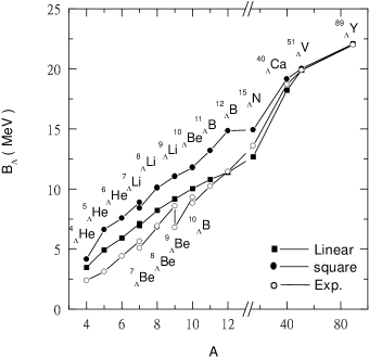
FIG. 11.: Hypernuclei binding energies $B_{\Lambda}$ calculated with linear and square root treatments of effective baryon mass versus baryon number A.

TABLE IV.: The values of double-$\Lambda$ hypernuclei $B_{\Lambda\Lambda}$ and $\Delta B_{\Lambda\Lambda}$ in MeV.

nuclei	$B_{\Lambda\Lambda}$(L)	$B_{\Lambda\Lambda}$(S)	Exp. [41]	Exp. [42]	$\Delta B_{\Lambda\Lambda}$(L)	$\Delta B_{\Lambda\Lambda}$(S)	Exp. [41]	Exp. [42]
${}^{~{}6}_{\Lambda\Lambda}$He	11.45	15.21	10.9$\pm$0.8	7.25$\pm$0.19	1.61	1.97	4.7$\pm$1.0	1.01$\pm$0.20
${}^{10}_{\Lambda\Lambda}$Be	19.66	23.66	17.7$\pm$0.4	-	1.32	1.60	4.3$\pm$0.4	-
${}^{13}_{\Lambda\Lambda}$B	23.67	30.22	27.5$\pm$0.7	-	0.89	0.54	4.8$\pm$0.7	-

The binding energies of two lambdas $B_{\Lambda\Lambda}$ defined as

$$B_{\Lambda\Lambda}=M(^{A-2}Z)+2M_{\Lambda}-M(^{A}_{\Lambda\Lambda}Z)$$ (58)

are listed in table IV. One can see that for the square root ansatz for baryon mass, the calculated results are several MeV larger compared with the old experimental values [41]. The linear definition improves this result. There are two reports for the new events of the production and detection of the double lambda hypernuclei [42, 43]. It shows that $B_{\Lambda\Lambda}$ of ${}^{~{}6}_{\Lambda\Lambda}$He is much smaller than the old value[42]. This new event was discussed in detail in Ref. [44]. The $\Lambda$-$\Lambda$ interaction energy $\Delta B_{\Lambda\Lambda}$ is defined as $\Delta B_{\Lambda\Lambda}=B_{\Lambda\Lambda}-2B_{\Lambda}$. The calculated results of these two treatments are similar and much smaller than the old experimental values. $\Delta B_{\Lambda\Lambda}$ of ${}^{~{}6}_{\Lambda\Lambda}$He obtained in this model is comparable with the new result.

V summary

We have used an improved treatment of the c.m. motion in calculating the effective, in-medium, baryon mass in an investigation of infinite hadronic matter, finite nuclei and hypernuclei within the chiral $SU(3)$ quark mean field model. The results are compared with earlier results which used the square root ansatz for effective mass. Both treatments fit the saturation properties of nuclear matter and therefore, for densities lower than the saturation density, these two treatments give reasonably similar results. The $\Xi$ potential in hadronic matter is reproduced better in the square root ansatz for baryon mass, while the linear definition gives a better $\Lambda$ potential. As a result, the binding energy of $\Lambda$ hypernuclei calculated from the linear definition is better when compared with experimental values. The energy levels of finite nuclei are reasonable in both of the treatments. In the linear definition, the spin-orbit splitting is smaller than that in the square root case. This is caused by the different effective nucleon mass at saturation density. The spin-orbit splitting can be improved by going beyond the mean field approximation [37].

For high baryon density, the predictions of these two treatments are quite different. There is a phase transition of chiral symmetry restoration in the case of the square root ansatz for baryon mass. The physical quantities, such as effective baryon mass and energy per baryon change discontinuously at the critical density. In the linear case, no such transition occurs. The effective baryon masses decrease slowly at high density. The different behavior at high density will result in significant difference for high density physics. It is therefore of interest to study the properties of neutron stars with these two treatments and to try to construct clearer theoretical motivations for possible definitions of the effective baryon mass. This will be done in the future.

REFERENCES

- [1] J. D. Walecka, Ann. Phys. 83 (1974) 491; S. A. Chin and J. D. Walecka, Phys. Lett. B 52 (1974) 24.
- [2] J. Zimanyi and S. A. Moszkowski, Phys. Rev. C 42 (1990) 1416.
- [3] A. R. Bodmer, Nucl. Phys. A 526 (1991) 703.
- [4] P. A. M. Guichon, Phys. Lett. B 200 (1988) 235; S. Fleck, W. Bentz, K. Shimizu and K. Yazaki, Nucl. Phys. A 510 (1990) 731; K. Saito and A. W. Thomas, Phys. Lett. B 327 (1994) 9. P. G. Blunden and G. A. Miller, Phys. Rev. C 54 (1996) 359. H. Müller and B. K. Jennings, Nucl. Phys. A 640 (1998) 55.
- [5] A. W. Thomas, S. Theberge and G. A. Miller, Phys. Rev. D 24 (1981) 216; A. W. Thomas, Adv. Nucl. Phys. 13 (1984) 1; G. A. Miller, A. W. Thomas and S. Theberge, Phys. Lett. B 91 (1980) 192.
- [6] H. Toki, U. Meyer, A. Faessler and R. Brockmann, Phys. Rev. C 58 (1998) 3749.
- [7] W. Bentz and A. W. Thomas, Nucl. Phys. A 696 (2001) 138. M. Buballa, hep-ph/0402234.
- [8] E. K. Heide, S. Rudaz, and P. J. Ellis, Nucl. Phys. A 571 (1994) 713.
- [9] G. Carter, P. J. Ellis, and S. Rudaz, Nucl. Phys. A 603 (1996) 367; Erratum-ibid. A 608 (1996) 514.
- [10] R. J. Furnstahl, H. B. Tang, and B. D. Serot, Phys. Rev. C 52 (1995) 1368.
- [11] I. Misbustin, J. Bondorf, and M. Rho, Nucl. Phys. A 555 (1993) 215.
- [12] P. Papazoglou, J. Schaffner, S. Schramm, D. Zschiesche, H. Stöcker, and W. Greiner, Phys. Rev. C 55 (1997) 1499.
- [13] L. L. Zhang, H. Q. Song, P. Wang, and R. K. Su, Phys. Rev. C 59 (1999) 3292.
- [14] P. Wang, Phys. Rev. C 61 (2000) 054904.
- [15] W. L. Qian, R. K. Su and P. Wang, Phys. Lett. B 491 (2000) 90.
- [16] P. Papazoglou, S. Schramm, J. Schaffner-Bielich, H. Stöcker and W. Greiner, Phys. Rev. C 57 (1998) 2576.
- [17] P. Papazoglou, D. Zschiesche, S. Schramm, J.Schaffner-Bielich, H. Stöcker and W. Greiner, Phys. Rev. C 59 (1999) 411.
- [18] P. Wang, Z. Y. Zhang, Y. W. Yu, R. K. Su and H. Q. Song, Nucl. Phys. A 688 (2001) 791.
- [19] P. Wang, H. Guo, Z. Y. Zhang, Y. W. Yu, R. K. Su and H. Q. Song, Nucl. Phys. A 705 (2002) 455.
- [20] P. Wang, Z. Y. Zhang, Y. W. Yu, Commun. Theor. Phys. 36 (2001) 71.
- [21] P. Wang, V. E. Lyubovitskij, Th. Gutsche and Amand Faessler, Phys. Rev. C 67 (2003) 015210.
- [22] P. Wang, H. Guo, Y. B. Dong, Z. Y. Zhang and Y. W. Yu, J. Phys. G 28 (2002) 2265.
- [23] P. A. M. Guichon, K. Saito, E. Rodionov and A. W. Thomas, Nucl. Phys. A 601 (1996) 349.
- [24] E. J. Hackett-Jones, D. B. Leinweber and A. W. Thomas, Phys. Lett. B 494 (2000) 89.
- [25] D. J. Millener, C. B. Dover and A. Gal, Phys. Rev. C 38 (1988) 2700.
- [26] D. E. Lanskoy and Y. Yamamoto, Phys. Rev. C 57 (1997) 2330.
- [27] T. Fakuda ., Phys. Rev. C 58 (1998) 1306.
- [28] P. Khaustov ., Phys. Rev. C 61 (2000) 054603.
- [29] J. Schaffner, C.B. Dover, A. Gal, C. Greiner, D.J. Millener, and H. Stöcher, Ann. Phys. 235 (1994) 35;
- [30] C. B. Dover, D. J. Millener and A. Gal, Phys. Rep. 184 (1989) 1.
- [31] I. Vidan̈a, A. Polls, A. Ramos, M. Hjorth-Jensen and V. G. J. Stoks, Phys. Rev. C 61 (2000) 025802.
- [32] J. Mares, E. Friedman, A. Gal and B. K. Jennings, Nucl. Phys. A 594 (1995) 311.
- [33] P. K. Saha . nucl-ex/0405031.
- [34] P. Wang, V. E. Lyubovitskij, Th. Gutsche and Amand Faessler, Phys. Rev. C 70 (2004) 015202.
- [35] J. Schaffner and A. Gal, Phys. Rev. C 62 (2000) 034311.
- [36] V. G. J. Stoks and T. S. H. Lee, Phys. Rev. C 60 (1999) 024006.
- [37] T. S. Biro and J. Zimanyi, Phys. Lett. B 391 (1997) 1. G. Krein, A. W. Thomas and K. Tsushima, Nucl. Phys. A 650 (1999) 313. P. A. M. Guichon and A. W. Thomas, nucl-th/0402064. R. J. Furnstahl, J. J. Rusnak and B. D. Serot, Nucl. Phys. A 632 (1998) 607.
- [38] K. Tsushima, K. Saito, J. Haidenbauer and A. W. Thomas, Nucl. Phys. A 630 (1998) 691; K. Tsushima, K. Saito and A. W. Thomas, Phys. Lett. B 411 (1997) 9, Erratum-ibid. B 421 (1998) 413
- [39] R. E. Chrien, Nucl. Phys. A 478 (1988) 705c.
- [40] M. Juric ., Nucl. Phys. B bf 52 (1973) 1.
- [41] G. B. Franklin, Nucl. Phys. A 585 (1995) 83c.
- [42] H. Takahashi ., Phys. Rev. Lett. 87 (2001) 212502.
- [43] J. K. Ahn ., Phys. Rev. Lett. 87 (2001) 132504.
- [44] I. N. Filikhin and A. Gal, Phys. Rev. C 65 (2002) 041001.