The Renormalisation Group and Applications in Few-Body Systems

yesyes This thesis is about effective field theories. We study the distorted wave renormalisation group (DWRG), a tool for constructing power-counting schemes in systems where some diagrams must be summed to all orders. We solve the DWRG equation for a variety of long-range potentials including the Coulomb, Yukawa and inverse square. We derive established results in the case of the Yukawa and Coulomb potentials and new results in the case of the inverse square potential. We generalise the DWRG to systems of three bodies and use it to find the power-counting for the three-body force in the KSW EFT. This power-counting corresponds to perturbations in the renormalisation group about a limit-cycle. We also derive equations for the LO and NLO KSW EFT distorted waves for three bosons and for three nucleons in the ${}^{3}S_{1}$ channel. The physical results in the nuclear system agree well, once the LO three-body force is determined, with predictions of more sophisticated potential models.

Declaration

No portion of the work referred to in this thesis has been submitted in support of an application for another degree or qualification at this or any other university or other institution of learning.

Copyright and Ownership of Intellectual Property Rights

1. Copyright in the text of this thesis rests with the Author. Copies (by any process) either in full, or of extracts, may be made only in accordance with instructions given by the Author and lodged in the John Rylands University Library of Manchester. Details may be obtained from the Librarian. This page must form part of any such copies made. Further copies (by any process) of copies made in accordance with such instructions may not be made without the permission (in writing) of the Author.

2. The ownership of any intellectual property rights which may be described in this thesis is vested in the University of Manchester, subject to any prior agreement to the contrary, and may not be made available for use by third parties without the written permission of the University, which will prescribe the terms and conditions of any such agreement.

Further information on the conditions under which disclosures and exploitation may take place is available from the Head of the Department of Physics and Astronomy.

Autobiographical Note

The author, Thomas Barford was born in Northampton in October 1977. He stayed in that grand town of rugby and Carlsberg until starting a Masters degree in Mathematics and Physics at the University of Warwick in 1996. Fours years and 273 hangovers later, having gained a first, he started a PhD in the theoretical physics at the University of Manchester. He has recently married a marvellous girl called Clare and they are very happy.

Publications

T. Barford and M. C. Birse,
“A renormalisation-group approach to two-body scattering with long-range forces,”
AIP Conf. Proc.  603 (2001) 229 [arXiv:nucl-th/0108024].

T. Barford and M. C. Birse,
“A renormalisation group approach to two-body scattering in the presence of long-range forces,”
Phys. Rev. C 67 (2003) 064006 [arXiv:hep-ph/0206146].

T. Barford and M. C. Birse,
“An effective field theory for the three-body system,”
Few Body Syst. Suppl.  14 (2003) 123 [arXiv:nucl-th/0210084].

Dedication

To Bella.

Chapter 1 Introduction

From an historical perspective, the hierarchy of scales to be found in the universe has controlled the development of physics since the middle ages. Time and again the theories of the past have been found to be only effective theories that approximate the physical world.

The first great post-Renaissance physics theory, Newtonian mechanics, is still used extensively in many areas, yet it has been ‘known’ for a long time that it is only an approximation. The advent of relativistic mechanics brought fresh insight into the nature of the universe as well as explaining some mysterious behaviour in the orbit of the planet Mercury, yet its use in explaining the path of a cricket ball struck through mid-wicket has never been advocated. Relativistic mechanics is a far more complicated beast than its ‘lesser’ cousin, in many cases the pay-off for the extra work involved in a calculation is simply not worth it. The difference in the path of that cricket ball as explained by Newtonian and relativistic mechanics would be unmeasurable.

Even though Newtonian mechanics is not fundamental to the nature of the universe as we know it now, it is still an effective theory; it explains what we see at speeds far below the speed of light, $c$. In quantifying this statement we might say that the difference between any classical or relativistic calculation, in which the typical speed is of order $v$, is of order $v^{2}/c^{2}$. We may then consider any problem, and knowing how accurately we want the result, chose between a full relativistic calculation, a simple classical calculation or maybe some middle ground in which the classical result is corrected to some order in $v^{2}/c^{2}$.

This kind of idea pervades physics today but nowhere is its importance as pronounced as in particle physics. Although the domain of particle physics may off-handedly be described as the study of the very small, the range of energies that are scrutinised, from the neutrino mass to the unification scale, far outstrips any other area of physics.

The first great triumph of quantum mechanics, the theory of the very small, was the calculation of the spectra of the hydrogen atom. However, the need for corrections to this result was soon apparent and there followed calculations for the fine structure, Lamb shift and hyperfine structure, each of which relied upon some previously unconsidered higher scale physics: spin-orbit coupling, relativistic corrections, loop diagrams in QED and dipole interactions. Despite all the corrections made in this calculation there are yet more that can be made, such as corrections due to the finite charge radius of the proton. An estimate of the magnitude of such a correction can be made in a similar way to the estimate of the relativistic corrections above. The corrections are expected to be of the order of $r_{p}^{2}/a_{0}^{2}$ where $r_{p}\sim 10^{-16}$m is the charge radius of the proton and $a_{0}=5.29\times 10^{-11}$m is the Bohr radius and an estimate of the typical distance of a ground state electron from the proton. Hence we expect a correction of the order $\Delta E\sim 10^{-9}E$. The key point here is the seemingly innocuous term ‘of the order of’. What do we mean by ‘of the order of’?

Arguments, like the one above, that involve using a separation of scales and expressions like ‘of the order of’ are implicitly assuming ‘naturalness’. The assumption of naturalness in these arguments is absolutely essential, without it nothing can be said about corrections such as relativistic corrections. In a nutshell one might say that the assumption of naturalness means that the coefficient, $b$, of for example the relativistic correction $\delta=bv^{2}/c^{2}$, is of order unity. That is, the number $b$, which is governed by the dynamics and geometry of the problem, is not so large or small to significantly change the size of the correction so that expressions like ‘of the order of’ apply.

Naturalness is not something that can necessarily be taken for granted, and indeed some fluke of the parameters may change the face of the problem, resulting in unexpected effects such as resonances.

It is only comparatively recently that physicists have sought to use the separations of scales in particle physics quantitatively to produce what have become known as effective field theories (EFTs) [1, 2, 3, 4, 5, 6]. In an EFT we seek to write down a low-energy equivalent of some ‘true’ higher energy theory. The concept was first introduced by Weinberg [7] in an attempt to use the near chiral symmetry of quantum chromodynamics (QCD) and the resulting separation of scales between the pion mass, $m_{\pi}$, and all other QCD scales to construct a low energy theory equivalent to QCD. Since this initial spark this idea has grown to become known as chiral perturbation theory (ChPT).

ChPT is defined by an effective Lagrangian that contains only those degrees of freedom explicit at the energies of interest, $Q\sim m_{\pi}$, i.e. pion fields and depending upon the particular problem, nucleon fields, hyper-nucleon fields etc. The fields are coupled by effective vertexes that contain the effects of all higher energy physics, of order $\Lambda_{0}$, not included in the Lagrangian, which is said to be ‘integrated out’. To include all of the integrated-out physics, the Lagrangian must include all terms not forbidden by the symmetries of the higher energy physics, invariably resulting in an infinite number of terms. To handle such a formidable Lagrangian the terms must be organised according to some ‘power-counting’ that assigns each term an order in an expansion in powers of $Q/\Lambda_{0}$. Any observable can be calculated to arbitrary accuracy by using the power-counting to include all the necessary terms.

In principle the effective couplings in the ChPT Lagrangian can be found by solving QCD, however, in practice they are determined by matching theory to a few experimental values, making the theory predictive in other areas.

In particle physics, the expression EFT was once synonymous with ChPT but it has since become an umbrella term for any number of theories in particle and atomic physics that subscribe to the same philosophy. Although EFTs are predominantly found in nuclear physics, where QCD is non-perturbative and hence almost impossible, they have been applied to areas as diverse as quantum gravity and string theory.

In studying nuclear systems at even lower energies than the pion mass, $Q\ll m_{\pi}$, we may integrate out the pionic degrees of freedom and deal with the pionless EFT in which the only degrees of freedom are the nucleon fields themselves. In this theory the underlying physics is that of the pion and the higher energy scale for the theory is the pion mass. The non-relativistic pionless EFT Lagrangian for nucleons of mass $M$ is given by,

$$\displaystyle{{\cal L}=N^{\dagger}\left(i\partial_{0}+\frac{\nabla^{2}}{2M}\right)N+\left[\frac{C_{0}}{4}|N|^{4}+\frac{C_{2}}{4}\left(N^{\dagger}(\overrightarrow{\nabla}-\overleftarrow{\nabla})^{2}N^{\dagger}\right)N^{2}+{\rm H.c.})+\ldots\right]}$$

$$\displaystyle{\qquad\qquad+\left[\frac{D_{0}}{36}|N|^{6}+\frac{D_{2}}{36}\left(N^{\dagger}(\overrightarrow{\nabla}-\overleftarrow{\nabla})^{2}N^{\dagger}\right)N^{\dagger}N^{3}+{\rm H.c.})+\ldots\right].}$$ (1.1)

It contains four point couplings denoted by $C_{2n}$ where $2n$ is the order of the field derivative at the vertex. Similarly, since they are not forbidden it contains six point couplings, denoted by $D_{2n}$, and eight point vertexes, ten point vertexes, etc. Relativistic corrections may be included by introducing higher order derivatives in the kinetic term [10].

Ignoring the six and higher point vertexes, which are not relevant to a two nucleon problem, we may immediately construct a power-counting to organise the terms in the effective Lagrangian using naive dimensional analysis, which inspired the power-counting in ChPT. The four point vertex couplings, $C_{2n}$, have dimension $-2-2n$. Since they describe physics that occurs at the order of the pion mass we may expect,

$$C_{2n}\sim\frac{1}{Mm_{\pi}^{2n+1}}.$$ (1.2)

In addition each loop between the vertexes contributes a term $\sim MQ/4\pi$. The order of any diagram involving any number of interactions can be evaluated by simply combining $n$ vertex terms with the $n-1$ loops in between. A diagram in which the $i^{\rm th}$ vertex contains $v_{i}$ derivatives will occur at order $(Q/m_{\pi})^{d}$ where,

$$d=n-1+\sum_{i=1}^{n}v_{i}.$$ (1.3)

This power-counting is known as the Weinberg scheme [8]. Unfortunately, when this organisation of the terms is used to describe the two-nucleon system it fails. The problem is the implicit assumption of naturalness.

Empirically, we observe in the two nucleon system a low-energy bound state, the deuteron, which has binding momentum $\gamma_{d}=45.7$Mev$\ll m_{\pi}$. The existence of this and the low energy resonances in the other isospin channels alerts us at once to some fine tuning of the parameters in the EFT. This fine tuning means that the naive dimensional analysis that results in the Weinberg scheme is no longer applicable. Some other power-counting must be found if we are to handle the infinite number of terms in the effective Lagrangian and produce the low-energy resonances [8, 9, 10, 11, 12, 13].

A new power-counting that resolved the problem was first introduced by Kaplan, Savage and Wise (KSW) [9] using the power divergence subtraction scheme (PDS) but found independently by van Kolck [10]. The PDS scheme introduces a new scale, $\mu$, which may be chosen to produce the fine tuning effects seen in the two nucleon system. Using the PDS scheme the scaling of the coefficients in the effective Lagrangian may be given as [9]

$$C_{2n}\sim\frac{1}{M\mu^{n+1}m_{\pi}^{n}}.$$ (1.4)

By choosing $\mu\sim Q$ we introduce the new low-energy scale required. Subsequently the term $C_{0}$ occurs at order $Q^{-1}$ and so all diagrams containing only the $C_{0}$ vertex must be summed to all orders. All other interactions scale with the negative powers of $m_{\pi}$ and so may be dealt with perturbatively provided each diagram is dressed with $C_{0}$ interaction bubbles. (Since an arbitrary number of $C_{0}$ interactions before or after the diagram does not change its order.) The subsequent power-counting is given by,

$$d=-2+\sum_{i=1}^{n}v_{i}.$$ (1.5)

This KSW power-counting is able to produce the low-energy resonances of order $\mu$ seen in nuclear systems.

The origin of these two different power-counting schemes can, in one way, be understood by using the renormalisation group (RG) [14]. The effective Lagrangian contains, by its very definition, an infinite number of non-renormalisable couplings. These result in divergent loop integrals which must be regularised, with a sharp momentum cut-off, $\Lambda$, for example, and then renormalised by absorbing all cut-off dependence into the effective couplings. In the context of EFTs the cut-off, $\Lambda$, is far more than a UV regulator, it ‘floats’ between the low-energy physics and the high-energy physics and allows us to control the introduction of high-energy physics and construct power-counting schemes. After rescaling all low-energy scales in terms of $\Lambda$, we are led to the concept of Wilson’s continuous RG [15] initially conceived for use in condensed matter theory. The RG describes how the couplings in the theory change as $\Lambda$ is varied.

The use of a sharp momentum cut-off leads us to a very intuitive idea of the RG flow. As $\Lambda$ gets smaller, more and more of the high energy physics is ‘integrated out’ and absorbed into the couplings of the EFT. Finally as $\Lambda$ reaches zero, all high energy physics is removed and all that remains is the rescaled low-energy physics, embodied in an infra-red fixed point of the RG. By perturbing about the IR fixed point with powers of $\Lambda$ we introduce dimensioned constants of integration that must scale with the high-energy scale $m_{\pi}$. In this way we can re-introduce high-energy physics into the couplings and create a power-counting scheme associated with that fixed point.

In chapter 2 we will study the RG for the two-body pionless EFT and reproduce the results of Birse et al [14] that reveal two fixed point solutions, a so-called trivial fixed point, which is associated with the Weinberg power-counting scheme and a non-trivial fixed point, which is associated with the KSW power-counting scheme. The constants of integration in the energy dependent perturbations around the trivial fixed point are in one-to-one correspondence with the terms in the Born expansion. Those around the non-trivial fixed point are in one-to-one correspondence with the effective range expansion [16].

The two-nucleon pionless EFT is a simple example that demonstrates the use of the RG in determining power-counting schemes. However, it is clearly not applicable for the interaction of two protons because of their electromagnetic interaction. Photon exchange between two protons has the characteristic energy scale,

$$\kappa=\frac{\alpha M}{2}=3.42\text{MeV},$$ (1.6)

where $\alpha$ is the fine structure constant and $M$ is the mass of the proton. In an EFT for protons below the pion mass $\kappa$ must be considered a low energy scale. All single photon exchange diagrams must, therefore, be included to all orders. However, as with the KSW power-counting, summing some diagrams to all orders and dressing others with ‘Coulomb bubbles’ may completely change the power-counting.

In chapter 3 we will introduce the distorted wave renormalisation group (DWRG) [17] and use it to study, as a first example, proton-proton scattering. The DWRG allows us to sum some low energy physics and absorb it into the fixed points of the RG. In particular we study a system of two particles interacting via some known long-range potential, equivalent to the sum of all known non-perturbative diagrams in the EFT, and a short-range potential, equivalent to all the shorter range interactions. By working in the basis of the distorted waves (DWs) of the long-range potential we show how to separate the effects of the long and short range potentials and then to construct a power-counting for the shorter range interactions.

The long range potential for the first example in chapter 3 will be the Coulomb potential. We will again find two fixed points, a trivial and a non-trivial associated with Weinberg and KSW -like schemes respectively. The integration constants in the perturbative series about these fixed points are found to be in a one-to-one correspondence with the terms in the distorted wave Born [18] and Coulomb modified effective range [19, 20, 21] expansions.

In the remainder of chapter 3 we will consider two more examples. Firstly, the repulsive inverse square potential, which is important to the extension of the pionless KSW EFT to three bodies and study of the power-counting in higher partial waves. This example is also interesting because it produces novel power-counting schemes that are very different to the schemes that are seen in the Coulomb DWRG and the ordinary RG.

Secondly, we shall consider a general example of “well-behaved” potentials, which includes among many others the Yukawa potential that may be used to include one pion exchange (OPE) in a nucleon-nucleon EFT. The solution of this DWRG has much in common with the solution of the Coulomb DWRG. This general analysis allows us to construct a general method for solving DWRG equations that will prove extremely useful in later applications. We conclude the chapter with the discussion of how to introduce explicit pions into an EFT for two nucleons.

After establishing the DWRG we shall look towards using it in the KSW EFT for three bodies. As outlined above, the KSW EFT is appropriate for systems with a low energy bound state or resonance that constitutes a new low energy scale in the problem. This low energy scale is characterised by an unusually large scattering length $1/a\sim Q\ll\Lambda_{0}$. Since this is a low energy scale its effects must be summed to all orders [22, 23, 24] and results in our need to use the DWRG.

Efimov [25] studied systems of three bodies with pairwise interactions characterised by a large scattering length, $a$, and zero effective range. He showed that these systems are similar to a two dimensional problem with an inverse square potential. This similarity occurs when the characteristic distance between the three particles $R\ll a$ and the problem essentially becomes scale free. In the limit of $a\rightarrow\infty$ the system is described exactly by an inverse square potential. The strength of the inverse square potential is determined purely by the statistics in the system. In the case of three s-wave Bosons and three s-wave nucleons in the ${}^{3}S_{1}$ channel the potential is attractive and singular. The singular nature of these potentials has a couple of interesting effects. Firstly, the Thomas effect [26]: the system will be no ground state, something first noted by Thomas as long ago as 1935. Secondly, in the limit of infinite scattering length, there will be an accumulation of geometrically spaced bound states at zero energy, known as Efimov states [25].

As the first step towards understanding the KSW EFT for three bodies, in chapter 4 we will look at the DWRG for the attractive inverse square potential. The singular nature of this potential means that without special measures the Hamiltonian is not self-adjoint. To construct a complete set of DWs we must construct a self-adjoint extension to the Hamiltonian [27, 28, 29] equivalent to defining some boundary condition near the origin. The connection to the three-body KSW EFT means that the singular nature of this potential has once more come under scrutiny [30, 31, 32], in particular with respect to understanding the link between the required self-adjoint extension and the three-body force.

The solution of the DWRG equation for the singular inverse square potential reveals that the self-adjoint extension is in fact equivalent to a marginal perturbation in the DWRG. The general method for solving the DWRG outlined at the end of chapter 3, augmented with some special considerations for the bound states, will reveal that the RG flow is controlled by limit-cycle solutions that evolve logarithmically in $\Lambda$.

In chapter 5 we will look at the extension of the DWRG to three body forces (3BDWRG). The 3BDWRG equation is more complex than the standard DWRG because of the multi-channelled nature of the system. The 3BDWRG equation has to describe the coupling of the three-body force to each of the channels. Fortunately the lessons learnt in chapters 3 and 4 allow us to find solutions.

We will demonstrate the solution of the 3BDWRG in an example of “well-behaved” pairwise forces and briefly show how the fixed points correspond to Weinberg and an equivalent KSW counting for three body forces. More interestingly we will look to the derivation of the power-counting for the three-body forces in the KSW EFT.

The nature of the three-body force in this system is still open to debate. The similarity to the singular inverse square potential is clear and the need for a self-adjoint extension is almost universally supported [30, 32]. It was hoped by some that effective range corrections of the two-body force would resolve the singular behaviour, however, results in this direction have failed to match experimental data [67].

Bedaque et al [22, 24] provide arguments in which they explicitly use a three-body force to define a self-adjoint extension and then continue to construct a power-counting for it. Phillips and Afnan [33] have shown how the inclusion of one piece of three-body data is enough to define all the physical variables without explicitly using a three-body force. These related approaches give results that are consistent with each other. Although the latter do not specify the actual nature of the three-body force it is clear that the inclusion of a piece of three-body data defines a self-adjoint extension of the Hamiltonian and is therefore equivalent to the leading-order (LO) three-body force given by Bedaque et al.

A third view is given by Gegalia and Blankleider[34] who argue that a unitarity constraint is sufficient to define physical quantities with no need for any three-body data at all. However, they have failed to produce any results that can be used to check the validity of their approach.

Since three-body force terms are not forbidden by the observed symmetries they must be included in the EFT Lagrangian. The 3BDWRG solution for the three-body force shows that the self-adjoint extension defining term is equivalent to a LO marginal three-body force and, consistent with the results of Bedaque et al [22, 24], acts as limit-cycle. Our results also support the power-counting suggested by Bedaque et al.

Having established the power-counting for the three-body force in the pionless KSW EFT, in chapter 6 we derive expressions for the DWs in this system at LO and next-to-leading order (NLO). The equations for the DWs based upon the two-body interactions alone show the singular behaviour anticipated by Efimov. The insertion of the LO three-body force is most easily achieved in this equations by demanding some boundary condition on the DWs close to the origin. Initially we will derive expressions for a three Boson system but in order to produce physically interesting results we will extend the equations to deal with a three nucleon system, in particular a system of two neutrons and a proton which contains the two- and three- body bound states, the deuteron and the triton. The LO three-body force can be fixed by matching to the neutron-deuteron scattering length. The EFT can then be used to construct the triton wavefunction and neutron-deuteron scattering states below threshold.

Chapter 2 The Renormalisation Group for Short Range Forces

2.1 Introduction

In this chapter we will introduce the renormalisation group method for constructing EFTs [14]. As already observed, the two key ingredients of an EFT are a power-counting scheme and a separation of scales. The first of these allows organisation of the infinite number of terms that naturally occur in an effective field theory, the second ensures that these terms may be truncated to achieve the desired level of precision.

The separation occurs between the scale of the physics of interest, $Q$, and that of the underlying high-energy physics, $\Lambda_{0}$. The existence of a separation of scales is usually assumed with a particular physical system in mind. For example, in nucleon-nucleon scattering at energies well below the pion mass, there is a natural separation between the momenta of the incoming particles and the lowest energy component of the strong interaction, one pion exchange. Utilisation of such a separation leads to what has become known, in nuclear physics, as a pionless EFT, in which the only fields are those of the asymptotically free particles with no exchange particles [9, 10, 11, 35, 36].

We will consider a system of two non-relativistic identical particle scattering via an effective Lagrangian. For weakly interacting systems the terms in the expansion can be organised according to naive dimensional analysis, a term proportional to $(Q/\Lambda_{0})^{d}$ being counted as of order $d$. This is known as Weinberg power-counting and is familiar from chiral perturbation theory (ChPT) [8]. However, for strongly interacting systems there can be new low-energy scales which are generated by non-perturbative dynamics e.g. the very large s-wave scattering length in nucleon-nucleon scattering. In such cases we need to resum certain terms to all orders and arrive at a new power-counting scheme, KSW power-counting [9, 10, 11]. The origin and use of these schemes becomes quite transparent using the renormalisation group method. The contents of this chapter largely follows the work of Birse et al [14, 37]

2.2 The RG Equation

In a Hamiltonian formulation, the effective Lagrangian is written as a potential consisting of contact interactions, which in coordinate space takes the form of $\delta$-functions and their derivatives and in momentum space takes the form,

$$V({\bf k^{\prime},k},p)=C_{00}+C_{200}k^{\prime 2}+C_{020}k^{\prime 2}+C_{110}{\bf k.k^{\prime}}+C_{002}p^{2}+\ldots,$$ (2.1)

where $p=\sqrt{ME}$ is the on-shell momentum corresponding to the total energy $E$ in the centre of mass frame and $M$ is twice the reduced mass. We shall consider s-wave scattering only at this stage, then since $V$ must be independent of ${\bf k.k^{\prime}}$, $C_{110}=0$.

Scattering variables are found by solving a Lippmann-Schwinger (LS) equation. In particular we shall work with the reactance matrix, $K$, which is related to the phaseshift, $\delta$ by,

$$\frac{1}{K(p,p,p)}=-\frac{Mp}{4\pi}\cot\delta,$$ (2.2)

and solves the LS equation,

$$K(k^{\prime},k,p)=V(k^{\prime},k,p)+\frac{M}{2\pi^{2}}\fint_{0}^{\infty}q^{2}dq\frac{V(k^{\prime},q,p)K(q,k,p)}{p^{2}-q^{2}},$$ (2.3)

where the bar on the integral sign indicates a principal value prescription for the pole on the real axis. Unitarity of the $S$-matrix is ensured if the $K$-matrix is hermitian. The on-shell $T$ and $K$ matrices are related by

$$\frac{1}{K(p,p,p)}=\frac{1}{T(p,p,p)}+\frac{iMp}{4\pi}.$$ (2.4)

For short range potentials, it is well known that the inverse of the $K$-matrix may be written in terms of the effective range expansion, [16]

$$-\frac{4\pi}{M}\frac{1}{K(p,p,p)}=p\cot\delta=-\frac{1}{a}+\frac{1}{2}r_{e}p^{2}+\ldots$$ (2.5)

where $a$ is called the scattering length and $r_{e}$ the effective range. The effective range, as its name suggests, is related in an indirect manner to the range of the potential [18] (provided it is “smooth”).

For contact interactions the integral in Eqn. (2.3) is divergent. From the EFT point of view this is to be expected, the divergence occurs because we have allowed high momentum modes to probe the EFT beyond its range of validity. The solution is to remove the high momentum modes and incorporate their effects into the effective potential, $V$. Mathematically, we apply a cut-off, $\Lambda$, to the integral then derive a differential equation for $V(k^{\prime},k,p,\Lambda)$ based upon the constraint that $K$, the observable, is independent of that cut-off. Rather than acting as a UV regulator the cut-off acts as a separation scale and ‘floats’ between the low-energy scales, $Q$, and the higher energy scales, $\Lambda_{0}$. This leads us the concept of a Wilsonian renormalisation group (RG) [15]. The interesting limit is $\Lambda\rightarrow 0$, in which all high energy physics has been integrated out.

The regularised LS equation can be written in operator form as,

$$K(p)=V(p,\Lambda)+V(p,\Lambda)G_{0}^{P}(p,\Lambda)K(p),$$ (2.6)

where $G_{0}^{P}(p,\Lambda)$ indicates the free Green’s function with standing wave boundary conditions and sharp cut-off $\Lambda$. The first step towards an RG equation for $V$ is differentiating Eqn. (2.6) with respect to $\Lambda$ and then eliminating $K$ to obtain,

$$\frac{\partial V(p,\Lambda)}{\partial\Lambda}=-V(p,\Lambda)\frac{\partial G_{0}^{P}(p,\Lambda)}{\partial\Lambda}V(p,\Lambda).$$ (2.7)

Taking matrix elements and expanding the Green’s function this equation takes the form,

$$\frac{\partial V(k^{\prime},k,p,\Lambda)}{\partial\Lambda}=\frac{M}{2\pi^{2}}V(k^{\prime},\Lambda,p,\Lambda)\frac{\Lambda^{2}}{\Lambda^{2}-p^{2}}V(\Lambda,k,p,\Lambda).$$ (2.8)

To obtain the RG equation for $V$ we must now rescale all low energy scales with $\Lambda$. We define the rescaled potential $\hat{V}$ by,

$$\hat{V}(\hat{k}^{\prime},\hat{k},\hat{p},\Lambda)=\frac{M\Lambda}{2\pi^{2}}V(\Lambda\hat{k}^{\prime},\Lambda\hat{k}\Lambda\hat{p},\Lambda).$$ (2.9)

where $\hat{k}=k/\Lambda$, $\hat{k}^{\prime}=k^{\prime}/\Lambda$ and $\hat{p}=p/\Lambda$. The resulting RG equation is,

$$\Lambda\frac{\partial\hat{V}}{\partial\Lambda}=\hat{p}\frac{\partial\hat{V}}{\partial\hat{p}}+\hat{k}\frac{\partial\hat{V}}{\partial\hat{k}}+\hat{k}^{\prime}\frac{\partial\hat{V}}{\partial\hat{k}^{\prime}}+\hat{V}+\hat{V}(\hat{k}^{\prime},1,\hat{p},\Lambda)\frac{1}{1-\hat{p}^{2}}\hat{V}(1,\hat{k},\hat{p},\Lambda).$$ (2.10)

The reason for this rescaling is that it allows distinct treatments of the low-energy physics and the parameterisation of high-energy physics. To explain, let us consider solutions that are independent of $\Lambda$. These solutions, known as fixed points, are scale free since they are independent of the only scale in the problem. Therefore they must be related to the rescaled low energy physics and be independent of the unscaled high energy physics.

Fixed-point solutions provide systems in which only the low-energy physics has been included and it is this that provides the key to constructing power-counting schemes. Solving the RG equation in the region of a fixed point by perturbing about it in powers of $\Lambda$ introduces parameters that must scale in inverse powers of $\Lambda_{0}$, the scale of the high energy physics. The perturbations around a fixed point organise the effective couplings into a power-counting scheme.

Since a fixed point solution is independent of $\Lambda$, all solutions of the RG equation tend to one as $\Lambda\rightarrow 0$. We may classify fixed points by examining the stability of the perturbations about them as $\Lambda\rightarrow 0$. If all perturbations tend to zero as $\Lambda\rightarrow 0$, i.e they scale with positive powers of $\Lambda$, the fixed point is stable. If there are perturbations that scale with negative powers of $\Lambda$ then the fixed point is unstable. A perturbation that does not scale with $\Lambda$ is known as marginal, and as we shall see in later chapters is associated with logarithmic behaviour in the cut-off.

In this problem, we shall find two fixed points that are of particular interest. The first of these, which we shall refer to as the trivial fixed point, is simply the obvious solution $\hat{V}=0$. This solution corresponds to the scale free system in which no scattering occurs. We shall see that the power-counting associated with the fixed point is the Weinberg scheme. A second fixed point, which we shall refer to as the non-trivial fixed point, gives a scale free system in which there is a bound state at exactly zero energy. The power-counting associated with this fixed point is the KSW scheme.

Eqn. (2.1) and the assumption of s-wave scattering implies that $V$ should be an analytic function of $p^{2},k^{2},$ and $k^{\prime 2}$. These constraints constitute a boundary condition upon the RG equation, physically they follow because the energy is below all thresholds for production of other particles and that the effective potential should describe short-ranged interactions.

2.3 The Trivial Fixed Point

The Trivial fixed point solution is the $\Lambda$-independent solution $\hat{V}=0$. To examine the perturbations around it we write the potential as

$$\hat{V}(\hat{k},\hat{k}^{\prime},\hat{p},\Lambda)=C\Lambda^{\nu}\phi(\hat{k}^{\prime},\hat{k},\hat{p}),$$ (2.11)

insert it into the RG equation, linearise, and obtain the eigenvalue equation

$$\hat{p}\frac{\partial\phi}{\partial\hat{p}}+\hat{k}\frac{\partial\phi}{\partial\hat{k}}+\hat{k}^{\prime}\frac{\partial\phi}{\partial\hat{k}^{\prime}}+\phi=\nu\phi.$$ (2.12)

The solutions of this equation are easily found to be

$$\phi(\hat{k}^{\prime},\hat{k},\hat{p})=\hat{k}^{\prime 2l}\hat{k}^{2m}\hat{p}^{2n},$$ (2.13)

with RG eigenvalues $\nu=2(l+m+n)+1$. The analyticity boundary conditions imply that $l,m$ and $n$ must be non-negative integers, so that $\nu$ takes the values $1,3,5,\ldots$. The solution to the RG equation in the region of the trivial fixed point is

$$\hat{V}(\hat{k}^{\prime},\hat{k},\hat{p},\Lambda)=\sum_{l,m,n=0}^{\infty}\hat{C}_{lmn}\left(\frac{\Lambda}{\Lambda_{0}}\right)^{\nu}\hat{k}^{\prime 2l}\hat{k}^{2m}\hat{p}^{2n},$$ (2.14)

where the coefficients $\hat{C}_{lmn}$ have been made dimensionless by extracting the high-energy scale $\Lambda_{0}^{-\nu}$ and for a Hermitian potential we must take $\hat{C}_{lmn}=\hat{C}_{mln}$. Since all the RG eigenvalues are positive this fixed point is stable as $\Lambda\rightarrow 0$.

The RG eigenvalues, $\nu$, provide a systematic way to classify the terms in the potential. In unscaled units we can see how this provides us with a power-counting scheme and straight away identify the couplings in the naively dimensioned potential suggested in chapter 1:

$$V(k^{\prime},k,p,\Lambda)=\frac{2\pi^{2}}{M\Lambda_{0}}\sum_{l,m,n=0}^{\infty}\hat{C}_{lmn}\frac{k^{\prime 2l}k^{2m}p^{2n}}{\Lambda_{0}^{2(l+m+n)}}.$$ (2.15)

The power-counting scheme is the Weinberg scheme if we assign an order $d=\nu-1$ to each term in the potential. That this power-counting scheme is useful for weakly interacting systems now comes as no surprise considering its association with the trivial, or zero-scattering, fixed point.

The corresponding $K$-matrix is simply given by the first Born approximation, as higher-order terms from the LS equation are cancelled by higher-order terms in the potential from the full, nonlinear RG equation [14]. It is important to notice that terms of the same order in the energy, $p^{2}$, or momenta, $k^{2}$ or $k^{\prime 2}$, occur at the same order in the power-counting. It is therefore possible to swap between energy or momentum dependence in the potential without affecting physical (on-shell) observables.

2.4 The Non-Trivial Fixed Point

2.4.1 Momentum Independent Solutions

Let us consider a fixed point solution, $\hat{V}_{0}(\hat{p})$, that depends on the energy, $\hat{p}$, but not upon the momentum. It satisfies the RG equation

$$\hat{p}\frac{d\hat{V}_{0}}{d\hat{p}}+\hat{V}_{0}+\frac{\hat{V}_{0}^{2}}{1-\hat{p}^{2}}=0.$$ (2.16)

A convenient way to solve this equation, as well as other momentum-independent RG equations, is to divide through by $\hat{V}_{0}^{2}$ and obtain a linear equation for $1/\hat{V}_{0}$,

$$\hat{p}\frac{d}{d\hat{p}}\left(\frac{1}{\hat{V}_{0}}\right)-\frac{1}{\hat{V}_{0}}-\frac{1}{1-\hat{p}^{2}}=0.$$ (2.17)

This equation is satisfied by the basic loop integral,

$$\hat{J}(\hat{p})=\fint_{0}^{1}d\hat{q}\frac{\hat{q}^{2}}{\hat{p}^{2}-\hat{q}^{2}}=-\left[1-\frac{\hat{p}}{2}\ln\frac{1+\hat{p}}{1-\hat{p}}\right].$$ (2.18)

Since $\hat{J}(\hat{p})$ is analytic in $\hat{p}^{2}$ as $\hat{p}^{2}\rightarrow 0$ it is a valid solution to the RG equation. Hence we take $\hat{V}_{0}=1/\hat{J}$. We shall refer to this as the non-trivial fixed point. When $\hat{V}_{0}$ is inserted into the LS equation we obtain

$$K(p,p,p)^{-1}=0,$$ (2.19)

which corresponds to a system with a bound state at zero energy. Since the energy of the bound state is exactly zero, the system has no scale associated with it, which is why it is described by a fixed point of the RG.

To find the power-counting associated with this fixed point we look for perturbations. This task is considerably easy if we consider momentum independent solutions. We consider perturbations of the form

$$\frac{1}{\hat{V}(\hat{p},\Lambda)}=\frac{1}{\hat{V}_{0}(\hat{p})}+C\Lambda^{\nu}\phi(\hat{p}),$$ (2.20)

giving the eigenvalue equation,

$$\hat{p}\frac{\partial\phi}{\partial\hat{p}}-\phi=\nu\phi.$$ (2.21)

Notice that since the momentum independent RG equation for $1/\hat{V}$ is linear, no approximation has been made to obtain eqn.(2.21). The potential obtained using these perturbations will be an exact solution to the RG equation. The eigenvalue equation is easy to solve:

$$\phi(\hat{p})=\hat{p}^{2n},$$ (2.22)

with RG eigenvalues $\nu=2n-1$. The analyticity boundary conditions demand that $n$ is a non-negative integer, so that the eigenvalues are $\nu=-1,1,3,\ldots$. The first eigenvalue is negative, which means that the fixed point is unstable as $\Lambda\rightarrow 0$. The full, momentum independent solution is given by

$$\frac{1}{\hat{V}(\hat{p},\Lambda)}=\frac{1}{\hat{V}_{0}(\hat{p})}+\sum_{n=0}^{\infty}\hat{C}_{2n-1}\left(\frac{\Lambda}{\Lambda_{0}}\right)^{2n-1}\hat{p}^{2n}.$$ (2.23)

The power-counting about this fixed point is the KSW scheme. As in the Weinberg case we assign each term an order $d=\nu-1$, so that the KSW scheme is characterised by the values $d=-2,0,2,\ldots$.

When this potential is inserted into the LS equation, we obtain an expression for the K-matrix, which upon using eqn.(2.2) gives the phaseshift,

$$p\cot\delta=-\frac{2\Lambda_{0}}{\pi}\sum_{n=0}^{\infty}\hat{C}_{2n-1}\left(\frac{p}{\Lambda_{0}}\right)^{2n}.$$ (2.24)

We can see that the terms in the expansion around the non-trivial fixed point are in one-to-one correspondence with the terms in the effective range expansion (2.5). In particular, we find

$$\hat{C}_{-1}=\frac{\pi}{2\Lambda_{0}a},\qquad\qquad\hat{C}_{1}=-\frac{\pi\Lambda_{0}r_{e}}{4}.$$ (2.25)

If the theory is natural then we expect the coefficients $\hat{C}_{2n-1}\sim 1$. In this case the scattering length and the effective range are of order $a\sim r_{e}\sim 1/\Lambda_{0}$.

Figure 2.1: The RG flow of the general momentum independent solutions, $\hat{V}(\hat{p},\Lambda)=\sum_{n=0}^{\infty}b_{2n}(\Lambda)\hat{p}^{2n}$. The fixed-points are shown as dots. The eigenvector flows are shown in bold with the arrows indicating flow as $\Lambda\rightarrow 0$. More general flows are shown as dashed.

To understand which of the two power-counting schemes is appropriate in a given situation, it is fruitful to examine the RG flow of purely energy dependent RG solutions illustrated in Fig.2.1. This figure shows the RG flow as $\Lambda\rightarrow 0$ in the plane $(b_{0}(\Lambda),b_{2}(\Lambda))$ where

$$\hat{V}(\hat{p},\Lambda)=b_{0}(\Lambda)+b_{2}(\Lambda)\hat{p}^{2n}+\ldots.$$ (2.26)

The trivial fixed point lies at $(0,0)$. All flows near to it flow into it as $\Lambda\rightarrow 0$, illustrating its already noted stability. The non-trivial fixed point lies at $(-1,-1)$, only flows lying on the critical line $b_{0}=-1$ flow into it. All other flows in the region of this critical line flow initially towards the non-trivial fixed point before the unstable perturbation becomes apparent and takes the flow into the domain of the trivial fixed point (possibly ‘via’ infinity).

The values of $\Lambda$ for which the flow is controlled by the non-trivial fixed point is dependent on the value of the coefficient $\hat{C}_{-1}$. In particular if

$$\Lambda>\frac{\pi}{2a}=\Lambda_{0}\hat{C}_{-1}$$ (2.27)

then the unstable perturbation is suppressed and the RG flow is controlled by the expansion around the non-trivial fixed point. As $\Lambda$ becomes less than $\pi/(2a)$ then the unstable perturbation becomes important and the flow moves away from the non-trivial fixed point and into the trivial fixed point.

In a natural theory we have $1/a\sim\Lambda_{0}$ so that as $\Lambda$ floats between the scale of the high energy physics, $\Lambda_{0}$, and $0$, the condition (2.27) is not met. This means that the RG flow is in the domain of the trivial fixed point and that the appropriate power-counting is the one obtained by perturbing about that point, the Weinberg scheme.

If there is some fine tuning in the theory so that $\hat{C}_{-1}$ is small, then the unstable perturbation is suppressed. This fine tuning, according to eqn. (2.25), will reveal itself in a surprisingly large scattering length, $a\gg 1/\Lambda_{0}$. As $\Lambda$ varies from $\Lambda_{0}$ to $1/a$ the condition (2.27) is true and the power-counting associated with the non-trivial fixed point provides a suitable expansion.

For example, in s-wave nucleon-nucleon scattering the scattering lengths are large suggesting a finely tuned effective potential with a small coefficient $\hat{C}_{-1}$, in this case the RG flow is dominated by the non-trivial fixed point and the power-counting associated with it, the KSW scheme, is the appropriate one to use in organising the terms [9, 10, 36, 11, 35].

2.4.2 Momentum Dependent Solutions.

In the analysis above the Weinberg and KSW counting schemes occur quite naturally. Study of the RG flow leads to conclusions about the usefulness of each of the schemes in different systems. However, the analysis is not complete as we have not considered the momentum dependent solution about the non-trivial fixed point.

Around the trivial fixed point, it was found that the momentum dependent perturbations provided no new physics since they occurred at the same order in the power counting as the energy dependent perturbations. This meant that momentum and energy perturbations could not be distinguished within on-shell observables.

Around the non-trivial fixed point things are considerably more complicated, as we shall see the momentum and energy dependent perturbations occur at different orders in the power counting. This result means that it is not a simple matter to interchange momentum and energy dependence of physical observables near the non-trivial fixed point.

To find the momentum dependent perturbations we write the solution in the vicinity of the fixed point solution as,

$$\hat{V}(\hat{k},\hat{k}^{\prime},\hat{p},\Lambda)=\hat{V}_{0}(\hat{p})+C\Lambda^{\nu}\phi(\hat{k},\hat{k}^{\prime},\hat{p}).$$ (2.28)

After linearising, the eigenvalue equation for $\phi$ is

$$\hat{p}\frac{\partial\phi}{\partial\hat{p}}+\hat{k}\frac{\partial\phi}{\partial\hat{k}}+\hat{k}^{\prime}\frac{\partial\phi}{\partial\hat{k}^{\prime}}+\frac{\hat{V}_{0}(\hat{p})}{1-\hat{p}^{2}}\left[\phi(\hat{k},1,\hat{p})+\phi(1,\hat{k}^{\prime},\hat{p})\right]=(\nu-1)\phi.$$ (2.29)

Useful solutions to this equation[37] are

$$\varphi_{n}(\hat{k},\hat{p})=\left[\hat{k}^{2n}-\hat{p}^{2n}+\sum_{l=0}^{n-1}\frac{\hat{p}^{2l}}{2(n-l)+1}\hat{V}_{0}(\hat{p})\right]\hat{V}_{0}(\hat{p}),$$ (2.30)

with eigenvalues, $\nu=2n=2,4,6,\ldots$. These solutions lead to two forms of perturbation that are symmetric in $k$ and $k^{\prime}$ and so may be used within an hermitian momentum dependent potential:

$$\phi(\hat{k},\hat{k}^{\prime},\hat{p})=\hat{p}^{2m}\left\{\varphi_{n}(\hat{k},\hat{p})+\varphi_{n}(\hat{k}^{\prime},\hat{p})\right\},$$ (2.31)

with eigenvalues $\nu=2m+2n=2,4,6,\ldots$ and

$$\phi(\hat{k},\hat{k}^{\prime},\hat{p})=\hat{p}^{2m}\left\{\varphi_{n}(\hat{k},\hat{p})\varphi_{n^{\prime}}(\hat{k}^{\prime},\hat{p})\right\},$$ (2.32)

with eigenvalues $\nu=2m+2n+2n^{\prime}+1=5,7,9,\ldots$. These perturbations plus the the purely energy dependent perturbations form a complete set that can be used to expand any perturbation about the non-trivial fixed point that is well-behaved as $\hat{k}^{2},\hat{k}^{\prime 2},\hat{p}^{2}\rightarrow 0$. The momentum dependent perturbations vanish on-shell and the terms in the on-shell potential are still in one-to-one correspondence with the terms in the effective range expansion[37]. The most general solution in the vicinity of the non-trivial fixed point may be written as

$$\displaystyle{\hat{V}(\hat{k},\hat{k}^{\prime},\hat{p},\Lambda)=\hat{V}_{0}(\hat{p})+\sum_{n=0}^{\infty}\hat{C}_{2n-1}\left(\frac{\Lambda}{\Lambda_{0}}\right)^{2n-1}\hat{p}^{2n}\hat{V}_{0}(\hat{p})^{2}+}$$

$$\qquad\displaystyle{\sum_{n=0,m=1}^{\infty}\hat{D}_{2(n+m)}\left(\frac{\Lambda}{\Lambda_{0}}\right)^{2(n+m)}\hat{p}^{2n}\left\{\varphi_{m}(\hat{k},\hat{p})+\varphi_{m}(\hat{k}^{\prime},\hat{p})\right\}+}$$

$$\qquad\qquad\displaystyle{\sum_{n=0;m,m^{\prime}=1}^{\infty}\hat{E}_{2(n+m+m^{\prime})+1}\left(\frac{\Lambda}{\Lambda_{0}}\right)^{2(n+m+m^{\prime})+1}\hat{p}^{2n}\varphi_{m}(\hat{k},\hat{p})\varphi_{m^{\prime}}(\hat{k}^{\prime},\hat{p}).}$$ (2.33)

When the on-shell $K$-matrix is calculated using this general form of expansion about the non-trivial fixed point, the only terms that contribute are precisely those that appear in the expansion given in the previous section, namely the coefficients of the purely energy dependent eigenfunctions, $\hat{C}_{\nu}$. The momentum dependent eigenfunctions do not contribute to on-shell scattering, i.e. physical observables are independent of $\hat{D}_{\nu}$ and $\hat{E}_{\nu}$ at this order [14, 37].

The solution given above results from linearisation of the RG equation close to the non-trivial fixed point. It is not clear that if a full solution to the non-linear RG equation was constructed that the one-to-one correspondence betweens terms in the potential and terms in the effective range expansion persists. In order to clarify the situation, Birse et al [14] calculated corrections to the potential around the non-trivial fixed point due to the neglected non-linear terms in the RG equation up to order $\hat{C}_{-1}\hat{D}_{2}$ and found the additional term,

$$\frac{\Lambda}{\Lambda_{0}}\hat{C}_{-1}\hat{D}_{2}\left(\hat{k}^{\prime 2}+\hat{k}^{2}+A\hat{p}^{2}+\frac{4\Lambda^{2}}{3}\hat{V}_{0}(\hat{p})\right)\hat{V}_{0}(\hat{p}),$$ (2.34)

where $A$ is a constant of integration. In general this second order piece will contribute to the effective range term along with the $\hat{C}_{1}$ term. Since the constant $A$ is unfixed, we are free to set it as we wish to ensure a nice correspondence between terms in the potential and terms in the effective range expansion. Setting $A=-2$ maintains the direct correspondence between the effective range expansion and the energy dependent perturbations around the non-trivial fixed point. In general it is assumed that at each order in the coefficients further degrees of freedom will become available to ensure this correspondence is continued to all orders.

The degrees of freedom that become available as the full non-linear solution is explored allows the possibility of generating the effective range terms from momentum dependent, rather than energy dependent, perturbations. For example, it is possible to generate the effective range, $r_{e}$, solely from the momentum dependence in the correction given in eqn. (2.34). By setting $\hat{C}_{1}=0$ and $A=0$ the effective range would be given by,

$$r_{e}=\frac{4\hat{D}_{2}}{\Lambda_{0}^{2}a}.$$ (2.35)

However, since the momentum dependent perturbations occur at different RG eigenvalues, $\nu=2,4,\ldots$, than the energy dependent perturbations they are replacing, the coefficient $D_{\nu}$ is forced to take an unnaturally large value to compensate for the additional factor of $\Lambda_{0}a$.

Unlike the trivial fixed point the possibility of using the equations of motion to move between momentum and energy dependence is not manifest at any particular order in the power-counting. This trade has to be between terms resulting from non-linear corrections in the solution to the RG equation in the vicinity of the fixed point, making it difficult to see and implement. Importantly, the momentum dependent perturbations offer no new degrees of freedom to on-shell observables than the easily elucidated energy dependent ones.

2.5 Summary

In this chapter we have introduced the RG for short range forces and used it to derive the Weinberg and KSW power-counting schemes. The key to solving the RG equation are fixed point solutions. Perturbing around the fixed point solutions gives us a simple recipe for constructing power-counting schemes. We have identified two fixed point solutions, the trivial fixed point that leads to the Weinberg scheme and a non-trivial fixed point that leads to the KSW scheme.

The terms in the perturbations around the trivial fixed point are in one to one correspondence with the terms in the DW Born expansion. Those about the non-trivial fixed point are in one-to-one correspondence with the terms in the effective range expansion.

By studying the RG flow with the cut-off $\Lambda$ we may make conclusions about the usefulness of each of the fixed points. The non-trivial fixed point is unstable and requires the fine tuning of a parameter in the expansion around it. This fine tuning results in large scattering lengths. Because of the large scattering lengths observed in nuclear systems the KSW counting is the appropriate scheme.

Chapter 3 The Distorted Wave Renormalisation Group

3.1 Introduction

In this chapter we shall introduce the distorted wave renormalisation group (DWRG) [17]. This is an extension of the RG which allows the summation of some physics to all orders.

The ability to construct an EFT with non-trivial low-energy physics is important. Consider proton-proton scattering at low energies. The Coulomb interaction between the protons is a very long-ranged interaction with a characteristic momentum scale, $\kappa=\frac{\alpha M}{2}=3.42\text{MeV}$. If we are interested in scattering between protons of typical energy $p\sim\kappa$, $\kappa$ must be treated as a low-energy scale, so we must sum all photon exchange diagrams since they occur at LO in the EFT [21].

Proton-proton scattering is not the only example that is important to nuclear physics. Also of interest is nucleon-nucleon scattering at energies comparable to the pion mass [45, 39, 38, 37]. In the previous chapter, we constructed a EFT in which all exchange particles are absorbed into the effective couplings. In nucleon-nucleon scattering the scale at which this breaks down is the pion mass, $m_{\pi}$, which acts as a high energy scale in the EFT. If we wish to examine nucleon-nucleon scattering at energies comparable to the pion mass, pion fields must be introduced into the EFT Lagrangian. Dependent upon our identification of low-energy scales, one approach may be to sum all one pion exchange diagrams [45]. There are many issues surrounding how pions are to be including in an EFT for nucleons [40, 49, 8, 50, 45], we shall consider these towards the end of this chapter.

We will introduce the DWRG equation by showing how the short and long range physics can be neatly separated. Then we will apply the equation to a number of examples. Our first example, in which the long-range physics will be modelled by the Coulomb potential, will demonstrate the methods that will be used in later examples. In the DWRG analysis of this system we will derive a known result for the distorted wave effective range expansion[19, 20, 21].

Our second example, will be the scale-free, repulsive inverse square potential. Our interest in this example is two-fold. Firstly, it will allow examination of short range forces for higher partial waves in the EFT for short range forces and secondly, the scale-free nature of the potential makes it very similar to three body systems[25].

As a final example we shall consider a more general class of long-range forces, namely non-singular potentials that facilitate the definition of the Jost function[18]. This general analysis is of interest as it includes the Yukawa potential and because the methodology used in this section acts as inspiration for the DWRG analysis in later chapters.

3.2 Separating Short- and Long-Range Physics

We shall assume that all non-perturbative EFT diagrams can be summed to give a long range potential. To this end, we consider a system of two-particles of mass $M$ interacting through the potential,

$$V=V_{L}+\tilde{V}_{S},$$ (3.1)

where $\tilde{V}_{S}$ is an effective short-range force that consists of contact interactions only. The terms in $\tilde{V}_{S}$ can be related to the couplings in the effective Lagrangian.

The full $T$-matrix that describes scattering from both the long and short range potentials is given by a LS equation,

$$T(p)=(V_{L}+\tilde{V}_{S})+(V_{L}+\tilde{V}_{S})G_{0}^{+}(p)T(p).$$ (3.2)

We wish to find an RG equation that allows us to determine the power-counting for the short range force. Suppose that we were to attempt to find this by applying the cut-off to the free Green’s function in eqn. (3.2). The resulting differential equation for $\tilde{V}_{S}$, found by demanding that $T$ is independent of $\Lambda$, is

$$\frac{\partial\tilde{V}_{S}}{\partial\Lambda}=-(V_{L}+\tilde{V}_{S})\frac{\partial G_{0}^{+}}{\partial\Lambda}(V_{L}+\tilde{V}_{S}).$$ (3.3)

After taking matrix elements we obtain an equation that in general contains complicated $\Lambda$-dependence in terms that are quadratic, linear and independent of $\tilde{V}_{S}$. In essence this complicated $\Lambda$-dependence is because of the cut-off, which applied to the free Green’s function in the LS equation, not only regularises the divergent loop integrals between contact interactions but also cuts-off elements of the long-range potential. Those parts of the long-range potential “removed” by the cut-off then have to be absorbed into the short-range potential resulting in the equation above, it then becomes difficult to justify any boundary condition on the potential, $\tilde{V}_{S}$.

To circumvent this complication and obtain an RG equation containing the short-range potential alone, it is useful to work in terms of the distorted waves (DWs), $|\psi_{\bf p}\rangle$, of the long-range potential. The DWs are simply solutions to the Schrödinger equation containing the long-range potential alone:

$$\left(H_{0}+V_{L}-\frac{p^{2}}{M}\right)|\psi_{\bf p}\rangle=0.$$ (3.4)

The $T$-matrix, $T_{L}$, describing scattering by $V_{L}$, is simply given by the LS equation:

$$T_{L}(p)=V_{L}+V_{L}G_{0}^{+}(p)T_{L}(p).$$ (3.5)

The corresponding full Green’s function is

$$G_{L}^{+}(p)=G_{0}^{+}(p)+G_{0}^{+}(p)T_{L}(p)G_{0}^{+}(p).$$ (3.6)

To isolate the effects of the short-range potential and enable a renormalisation group analysis we write the full $T$-matrix as [18]

$$T(p)=T_{L}(p)+(1+T_{L}(p)G_{0}^{+}(p))\tilde{T}_{S}(p)(1+G_{0}^{+}(p)T_{L}(p)).$$ (3.7)

The operator $(1+G_{0}^{+}T_{L})$ is the Möller wave operator that converts a plane wave into a DW of $V_{L}$,

$$|\psi_{\bf p}\rangle=(1+G_{0}^{+}(p)T_{L}(p))|{\bf p}\rangle,$$ (3.8)

so that the matrix elements of the full $T$-matrix are given by,

$$\langle{\bf k}|T(p)|{\bf k^{\prime}}\rangle=\langle{\bf k}|T_{L}(p)|{\bf k^{\prime}}\rangle+\langle\psi^{-}_{\bf k}|\tilde{T}_{S}(p)|\psi^{+}_{\bf k^{\prime}}\rangle.$$ (3.9)

An equation for the operator $\tilde{T}_{S}(p)$ can be found by substituting eqn. (3.7) into the full LS equation (3.2). After identifying and cancelling the terms in the pure long-range LS equation and cancelling the Möller wave operator on the right hand side we are left with,

$$\displaystyle{[1+T_{L}(p)G_{0}^{+}(p)]\tilde{T}_{S}(p)=\tilde{V}_{S}+\tilde{V}_{S}G_{0}^{+}(p)[1+T_{L}(p)G_{0}^{+}(p)]\tilde{T}_{S}(p)}$$

$$\displaystyle{\qquad\qquad\qquad\qquad\qquad\qquad\qquad+V_{L}G_{0}^{+}(p)[1+T_{L}(p)G_{0}^{+}(p)]\tilde{T}_{S}(p).}$$ (3.10)

The third term on the right-hand side can be seen to cancel with the second on the left-hand side after identifying the LS equation for $T_{L}$. The second term on the right hand side can be simplified by identifying the form for the full long-range Green’s function, eqn. (3.6). What remains is a distorted wave Lippmann-Schwinger (DWLS) equation for the $\tilde{T}_{S}$,

$$\tilde{T}_{S}(p)=\tilde{V}_{S}+\tilde{V}_{S}G_{L}^{+}(p)\tilde{T}_{S}(p).$$ (3.11)

This equation is now a far more promising starting point for the RG analysis since the effects of the long-range potential have been dealt with separately. The operator $\tilde{T}_{S}$ describes the interaction between the short-range potential and the DWs of the long-range potential

We shall assume that $V_{L}$ is a central potential and work in the partial wave basis. In particular we shall concentrate on s-wave scattering. In that case the on-shell $T$-matrix may be expressed in terms of the phaseshift,

$$\langle p|T(p)|p\rangle=-\frac{4\pi p}{M}\frac{e^{2i\delta}-1}{2i}.$$ (3.12)

A similar relation holds between $T_{L}$ and $\delta_{L}$, the phaseshift due to the long range potential alone. We may write the full phaseshift, $\delta$, as $\delta_{L}$ plus a correction, $\tilde{\delta}_{S}$, due to the effect of the short-range potential:

$$\delta=\delta_{L}+\tilde{\delta}_{S}.$$ (3.13)

Substituting this form into eqn. (3.12) and subsequently into eqn. (3.7) we obtain a simple relationship between the on-shell matrix elements of $\tilde{T}_{S}$ and the corrective phaseshift $\tilde{\delta}_{S}$,

$$\langle\psi^{-}_{p}|\tilde{T}_{S}(p)|\psi^{+}_{p}\rangle=-\frac{4\pi p}{M}e^{2i\delta_{L}(p)}\frac{e^{2i\tilde{\delta}_{S}(p)}-1}{2i}.$$ (3.14)

3.3 The DWRG equation

In order to derive the DWRG equation for the short-range potential it is once again more convenient to work with a reactance matrix, $\tilde{K}_{S}$, which satisfies the DWLS equation,

$$\tilde{K}_{S}(p)=\tilde{V}_{S}(p)+\tilde{V}_{S}(p)G_{L}^{P}(p)\tilde{K}_{S}(p),$$ (3.15)

where in this equation $G_{L}^{P}$ indicates the Green’s function with standing wave boundary conditions. The relationship between the on-shell matrix elements of $\tilde{T}$ and $\tilde{K}$ (c.f. eqn. (2.4) is,

$$\frac{1}{\langle\psi_{p}|\tilde{K}_{S}(p)|\psi_{p}\rangle}=\frac{e^{2i\delta_{L}(p)}}{\langle\psi^{-}_{p}|\tilde{T}_{S}(p)|\psi^{+}_{p}\rangle}+\frac{iM}{4\pi p},$$ (3.16)

where similarly $|\psi_{p}\rangle$ without superscript indicates standing wave boundary conditions on the DW. Hence the on-shell $\tilde{K}_{S}$-matrix is given by

$$\frac{1}{\langle\psi_{p}|\tilde{K}_{S}(p)|\psi_{p}\rangle}=-\frac{M}{4\pi p}\cot\tilde{\delta}_{S}.$$ (3.17)

To regulate eqn. (3.15) we expand $G_{L}^{P}$ using the completeness relation for the DWs, and apply a cut-off to the continuum states,

$$G_{L}^{P}(p,\Lambda)=\frac{M}{2\pi^{2}}\fint_{0}^{\Lambda}{\rm d}q\,\frac{|\psi_{q}\rangle\langle\psi_{q}|}{p^{2}-q^{2}}+\frac{M}{4\pi}\sum_{n}\frac{|\psi_{n}\rangle\langle\psi_{n}|}{p^{2}+p_{n}^{2}}.$$ (3.18)

Demanding that $\tilde{K}_{S}$ is $\Lambda$-independent we can obtain, as in the previous chapter, a differential equation for $\tilde{V}_{S}$ by differentiating eqn. (3.15) with respect to $\Lambda$ and eliminating $\tilde{K}_{S}$ to obtain,

$$\frac{\partial\tilde{V}_{S}}{\partial\Lambda}(p,\Lambda)=-\tilde{V}_{S}(p,\Lambda)\frac{\partial G_{L}^{P}}{\partial\Lambda}(p,\Lambda)\tilde{V}_{S}(p,\Lambda).$$ (3.19)

In the remainder of this chapter, to simplify the analysis, we shall assume that the matrix elements of $\tilde{V}_{S}$ depend only on the energy, $p$ and not on the momentum. As shown in chapter 2, the off-shell momentum dependent solutions to the RG equation have more complicated forms but are not needed to describe on-shell scattering [14, 37].

In the previous chapter we simply used a contact interaction proportional to a delta function, however, such a choice cannot be used in combination with some of the long-range potentials of interest. Long-range potentials that are sufficiently singular that their DWs, $\psi_{p}(r)$, either vanish or diverge as $r\rightarrow 0$ will result in a poorly defined DWRG equation if a delta function contact term is used.

To construct a contact interaction we chose a spherically symmetric potential with a short but nonzero range. By choosing the range, $R$, of this potential to be much smaller than $1/\Lambda$, we ensure that any additional energy or momentum dependence associated with it is no larger than that of the physics which has been integrated out, and hence the power-counting is not altered by it. The precise value of this scale is arbitrary and so observables should not depend on it, we may consider the results to be equivalent to those that would be obtained in the limit $R\rightarrow 0$. $R$ should be thought of nothing more than a tool to avoid a null DWRG equation. A simple and convenient choice for the form of the potential is the “$\delta$-shell” potential,

$$\tilde{V}_{S}(r)=V_{S}\delta(r-R).$$ (3.20)

With this choice, the eqn. (3.19) for $V_{S}$ becomes

$$\frac{\partial V_{S}(p,\kappa,\Lambda)}{\partial\Lambda}=-\frac{M}{2\pi^{2}}\frac{|\psi_{\Lambda}(R)|^{2}}{p^{2}-\Lambda^{2}}V_{S}^{2}(p,\kappa,\Lambda).$$ (3.21)

The final step in obtaining the DWRG equation is to rescale each of the low energy scales, expressing them in terms of the cut-off $\Lambda$. Dimensionless momentum variables are defined by $\hat{p}=p/\Lambda$ etc., along with a rescaled potential, $\hat{V}_{S}$. The exact nature of the rescaling required for the potential is dependent on the form of $\psi_{\Lambda}(R)$.

The solution to the DWRG equation should satisfy the analyticity boundary conditions in $\hat{p}^{2}$ that follow from the same arguments given in the previous chapter. $\hat{V}_{S}$ must also be analytic in any other low energy scale, $\kappa$, associated with the long-range potential. The exact analyticity condition for each scale $\kappa$ is case specific. In most cases we need to demand only that the effective potential is analytic in $\kappa$. An example is the inverse Bohr radius which is the low-energy scale associated with the Coulomb potential, and which is proportional to the fine structure constant, $\alpha$. Since the short-distance physics which has been incorporated in the effective potential should be analytic in $\alpha$ it should be analytic in $\kappa$. An important exception is the pion mass. This is proportional to the square root of the strength of the chiral symmetry breaking (the current quark mass in the underlying theory, QCD) and so, as in ChPT, the effective potential should be analytic in $m_{\pi}^{2}$. Under these restrictions, we see that $\hat{V}_{S}$ should have an expansion in non-negative, integer powers of $\hat{p}^{2}$ and $\hat{\kappa}$ (or $\hat{\kappa}^{2}$).

3.4 The Coulomb Potential

Having discussed the general route to the DWRG equation we shall now provide a concrete and physically interesting example to see how the whole procedure fits together. The Coulomb potential, $V_{L}(r)=\alpha r^{-1}$, is highly interesting physically for obvious reasons. The wavefunction for the Coulomb potential may be written in terms of the confluent hypergeometric function, $\Phi(a,b,z)$,

$$\psi_{p}^{(+)}(r)=pre^{-\frac{1}{2}\pi\eta}\Gamma(1+i\eta)\Phi(1+i\eta,2,-2ipr)e^{ipr},$$ (3.22)

where $\eta=\kappa/p$, $\kappa=\alpha M/2$[18]. The definition of the phaseshift for the Coulomb potential is unusual because the long $r^{-1}$ tail results in logarithmic asymptotic contributions. The Coulomb phaseshift is defined by writing the asymptotic behaviour of the wavefunction as,

$$\psi_{p}^{(+)}(r)\rightarrow e^{i\delta_{c}}\sin(pr-\eta\ln{2pr}+\delta_{c}),$$ (3.23)

which gives the phaseshift $\delta_{c}={\text{A}rg}\{\Gamma(1+i\eta)\}$. Incidentally, this expression also defines the normalisation of the DWs. A simple calculation shows that for $R\ll\Lambda^{-1}$ we have,

$$|\psi_{\Lambda}(R)|^{2}\rightarrow\Lambda^{2}R^{2}e^{-\pi\hat{\kappa}}\Gamma\left(1+i\frac{\kappa}{\Lambda}\right)\Gamma\left(1-i\frac{\kappa}{\Lambda}\right)=\frac{2\pi\kappa\Lambda R^{2}}{e^{2\pi\kappa/\Lambda}-1}=R^{2}\Lambda^{2}{\cal C}(\kappa/\Lambda).$$ (3.24)

where ${\cal C}(\eta)$ is known as the Sommerfeld factor. Hence, in the Coulomb case eqn. (3.21) becomes

$$\frac{\partial V_{S}(p,\kappa,\Lambda)}{\partial\Lambda}=-\frac{MR^{2}}{2\pi^{2}}{\cal C}(\kappa/\Lambda)\frac{\Lambda^{2}}{p^{2}-\Lambda^{2}}V_{S}^{2}(p,\kappa,\Lambda).$$ (3.25)

To obtain the DWRG equation we must rescale the variables $p=\hat{p}\Lambda$ and $\kappa=\hat{\kappa}\Lambda$. $V_{S}$ must be rescaled to factor out the scales $M$ and $R$. Hence we define,

$$\hat{V}_{S}(\hat{p},\hat{\kappa},\Lambda)=\frac{M\Lambda R^{2}}{2\pi^{2}}V_{S}(\Lambda\hat{p},\Lambda\hat{\kappa},\Lambda),$$ (3.26)

resulting in the DWRG equation for the Coulomb potential:

$$\Lambda\frac{\partial\hat{V}_{S}}{\partial\Lambda}=\hat{p}\frac{\partial\hat{V}_{S}}{\partial\hat{p}}+\hat{\kappa}\frac{\partial\hat{V}_{S}}{\partial\hat{\kappa}}+\hat{V}_{S}+\frac{{\cal C}(\hat{\kappa})}{1-\hat{p}^{2}}\hat{V}_{S}^{2}.$$ (3.27)

The boundary conditions that follow from the discussion above are analyticity about $\hat{p}^{2},\hat{\kappa}\rightarrow 0$. We shall assume that $\kappa$ is positive, i.e. that the Coulomb potential is repulsive, the modifications to this discussion for an attractive Coulomb potential are examined in Appendix B.

Our study of the Coulomb DWRG equation will mirror the RG analysis of the previous chapter. In particular we shall concern ourselves with fixed-point solutions and their corresponding power-counting schemes. A trivial fixed point, $\hat{V}_{S}=0$, is readily identified, but the existence of a non-trivial fixed point is not obvious. We will see that no true fixed point other than the trivial one exists. However, we will find a logarithmically evolving ‘fixed point’ that for the purpose of constructing a power-counting scheme may be regarded as a true fixed point. Furthermore, we will find a marginal perturbation in the RG flow about this fixed point that is associated with its logarithmic evolution.

3.4.1 The Trivial Fixed Point

An obvious fixed point solution of the DWRG equation for the Coulomb potential is the trivial fixed point solution, $\hat{V}_{S}=0$. This solution corresponds to a vanishing short-range force, i.e. a system in which only the Coulomb force is active. The power-counting associated with the point can be obtained by solving the eigenvalue equation for a small perturbation about it. Putting

$$\hat{V}_{S}(\hat{p},\hat{\kappa},\Lambda)=C\Lambda^{\sigma}\phi(\hat{p},\hat{\kappa}),$$ (3.28)

we obtain an eigenvalue equation that is very similar to that in the previous chapter,

$$\hat{p}\frac{\partial\phi}{\partial\hat{p}}+\hat{\kappa}\frac{\partial\phi}{\partial\hat{\kappa}}=(\nu-1)\phi.$$ (3.29)

The solutions that satisfy the boundary conditions are $\phi=\hat{p}^{2n}\kappa^{m}$, where $n$ and $m$ are positive integers. The RG eigenvalues are $\nu=2n+m+1=1,2,3,\ldots$. All the RG eigenvalues, in common with the pure short range case of the previous chapter, are positive and the fixed-point is stable. The potential in the vicinity of the fixed-point is given by,

$$\hat{V}_{S}=\sum_{n,m=1}^{\infty}\hat{C}_{2n,m}\left(\frac{\Lambda}{\Lambda_{0}}\right)^{2n+m+1}\hat{p}^{2n}\hat{\kappa}^{m}.$$ (3.30)

If we assign $d=\nu-1$ then the power-counting scheme is the Weinberg scheme with additional $\kappa$-dependent terms. Upon substitution into the Lippmann Schwinger Equation, all higher order terms vanish and what remains is a distorted wave Born Expansion,

$$\frac{\tan\tilde{\delta}_{S}}{p}=-\frac{\pi}{2\Lambda_{0}}{\cal C}(\eta)\sum_{n,m=1}^{\infty}\hat{C}_{2n,m}\left(\frac{p^{2n}\kappa^{m}}{\Lambda_{0}^{2n+m}}\right),$$ (3.31)

which, it should be noted, is independent of the delta-shell range, $R$. This power-counting scheme, in parallel to the trivial fixed point for purely short-range potentials, is appropriate for systems with weakly interacting short-range potentials that provide only minor corrections to the Coulomb potential.

3.4.2 The Non-Trivial Fixed Point

The starting point for finding another fixed point solution is to divide the DWRG equation through by $\hat{V}_{S}^{2}$ to obtain a linear PDE for $\hat{V}_{S}^{-1}$,

$$\Lambda\frac{\partial\hat{V}_{S}^{-1}}{\partial\Lambda}=\hat{p}\frac{\partial\hat{V}_{S}^{-1}}{\partial\hat{p}}+\hat{\kappa}\frac{\partial\hat{V}_{S}^{-1}}{\partial\hat{\kappa}}-\hat{V}_{S}^{-1}-\frac{{\cal C}(\hat{\kappa})}{1-\hat{p}^{2}}.$$ (3.32)

Substitution shows that this equation has a fixed point solution given by the basic loop integral,

$$\hat{J}(\hat{p},\hat{\kappa})=\fint_{0}^{1}\hat{q}^{2}d\hat{q}\frac{{\cal C}(\hat{\kappa}/\hat{q})}{\hat{p}^{2}-\hat{q}^{2}}.$$ (3.33)

However, we may not simply take $\hat{V}_{S}=\hat{J}^{-1}$ as the solution to the RG equation because it does not satisfy the necessary analyticity boundary conditions. A source of non-analyticity in $\hat{p}^{2}$ are the poles at $\hat{q}=\pm\hat{p}$. As $\hat{p}\rightarrow 0$ these poles move to the endpoint of the integral, $\hat{q}=0$, causing singular behaviour in $\hat{J}$. A second source of singular behaviour is the essential singularity in ${\cal C}(\eta)$ at $\eta=0$. This singularity means that the integral $\hat{J}$ only converges for $\text{Re}\{\hat{\kappa}\}>0$ resulting in singular behaviour about $\hat{\kappa}=0$. In order to isolate these non-analyticities we write $\hat{J}$ as:

$$\hat{J}(\hat{p},\hat{\kappa})=-\int_{0}^{1}d\hat{q}{\cal C}(\hat{\kappa}/\hat{q})-\hat{p}^{2}\int_{1}^{\infty}d\hat{q}\frac{{\cal C}(\hat{\kappa}/\hat{q})}{\hat{p}^{2}-\hat{q}^{2}}+\hat{\cal M}(\hat{p},\hat{\kappa}),$$ (3.34)

where

$$\hat{\cal M}(\hat{p},\hat{\kappa})=\hat{p}^{2}\fint_{0}^{\infty}d\hat{q}\frac{{\cal C}(\hat{\kappa}/\hat{q})}{\hat{p}^{2}-\hat{q}^{2}}.$$ (3.35)

The non-analyticity in $\hat{p}^{2}$ caused by the $\hat{q}=0$ endpoint now appears in $\hat{\cal M}$, whilst the non-analyticity resulting from the essential singularity in $\cal C$ is contained in both $\hat{\cal M}$ and the first integral in eqn. (3.34). The second integral in eqn. (3.34) avoids the troublesome endpoint, $\hat{q}=0$, and is analytic in both $\hat{\kappa}$ and $\hat{p}$. The first integral in eqn. (3.34) may be written as (see Appendix A),

$$-\int_{0}^{1}d\hat{q}\,{\cal C}(\hat{\kappa}/\hat{q})=-1-\pi\hat{\kappa}\ln\hat{\kappa}+\text{Analytic terms in $\hat{\kappa}$},$$ (3.36)

So that overall we have,

$$\hat{J}(\hat{p},\hat{\kappa})=\hat{\cal M}(\hat{p},\hat{\kappa})-\pi\hat{\kappa}\ln\hat{\kappa}+\text{Terms Analytic in $\hat{p}^{2},\hat{\kappa}$}.$$ (3.37)

To construct a solution to the DWRG fixed point equation that satisfies the analyticity boundary conditions we must remove the non-analytic terms $\hat{\cal M}$ and $\hat{\kappa}\ln\hat{\kappa}$. The removal of the non-analytic term $\hat{\cal M}$ is simple. It is not difficult to show that it satisfies the homogeneous form of eqn. (3.32),

$$\hat{p}\frac{\partial\hat{\cal M}}{\partial\hat{p}}+\hat{\kappa}\frac{\partial\hat{\cal M}}{\partial\hat{\kappa}}-\hat{\cal M}=0,$$ (3.38)

so that $\hat{J}-\hat{\cal M}$ satisfies eqn. (3.32). However, the removal of the logarithmic term in eqn. (3.36) is not as simple and cannot be done within the confines of the fixed point equation. It is because of this term that we are forced to introduce logarithmic $\Lambda$ dependence into the fixed point solution. The term,

$$\hat{\cal L}(\hat{\kappa},\Lambda)=-\pi\hat{\kappa}\ln\frac{\Lambda\hat{\kappa}}{\mu},$$ (3.39)

where $\mu$ is some arbitrary scale, satisfies the homogeneous form of the eqn. (3.32),

$$\Lambda\frac{\partial\hat{\cal L}}{\partial\Lambda}-\hat{\kappa}\frac{\partial\hat{\cal L}}{\partial\hat{\kappa}}+\hat{\cal L}=0,$$ (3.40)

and so may be used to remove the logarithmic term from $\hat{J}$. Bringing all the terms together we take

$$\hat{V}_{S}^{(0)}(\hat{p},\hat{\kappa},\Lambda)=\Bigl{(}\hat{J}(\hat{p},\hat{\kappa})-\hat{\cal M}(\hat{p},\hat{\kappa})-\hat{\cal L}(\hat{\kappa},\Lambda)\Bigr{)}^{-1}$$ (3.41)

as an analytic solution to the DWRG equation with logarithmic dependence on $\Lambda$. We will refer to this as the non-trivial fixed point .

The perturbations around the non-trivial fixed point can be found in the same way as before. Writing,

$$\frac{1}{\hat{V}_{S}(\hat{p},\hat{\kappa},\Lambda)}=\frac{1}{\hat{V}_{S}^{(0)}(\hat{p},\hat{\kappa},\Lambda)}+\Lambda^{\nu}\phi(\hat{p},\hat{\kappa}),$$ (3.42)

we obtain a linear equation for $\phi$ which is readily solved,

$$\phi(\hat{p},\hat{\kappa})=\hat{p}^{2n}\hat{\kappa}^{m},$$ (3.43)

where $n$ and $m$ are positive integers and the RG eigenvalues are $\nu=2n+m-1$. The leading order perturbation around this fixed point has a negative RG eigenvalue and so, like the non-trivial fixed point seen in the previous chapter, is unstable. Indeed, the power-counting in the energy dependent terms around this fixed point is simply the KSW scheme. In contrast to the power-counting observed there, the existence of a zero RG eigenvalue means that there is a marginal perturbation that does not scale with a power of $\Lambda$. The full solution in the vicinity of the non-trivial fixed point is,

$$\frac{1}{\hat{V}_{S}(\hat{p},\hat{\kappa},\Lambda)}=\frac{1}{\hat{V}_{S}^{(0)}(\hat{p},\hat{\kappa},\Lambda)}+\sum_{n,m=0}^{\infty}\hat{C}_{2n,m}\left(\frac{\Lambda}{\Lambda_{0}}\right)^{2n+m-1}\hat{p}^{2n}\hat{\kappa}^{m}.$$ (3.44)

The marginal perturbation is the key to understanding the need for logarithmic dependence on $\Lambda$ in the fixed point solution and the arbitrary scale $\mu$. Since the marginal perturbation is independent of $\Lambda$ it cannot be separated unambiguously from the fixed point solution $\hat{V}_{S}^{(0)}$. The degree of freedom associated with the scale $\mu$ is interchangeable with the coefficient $\hat{C}_{01}$. Indeed the coefficient, $\hat{C}_{01}$ can be chosen to depend on $\mu$ in such a way that the term,

$$\pi\hat{\kappa}\ln{\frac{\Lambda}{\mu}}+\hat{C}_{01}(\mu)\hat{\kappa},$$ (3.45)

and hence the full solution is independent of $\mu$.

This system is very similar to the case of considered in Chapter 2. The power-counting in the energy dependent terms around both fixed-points is the same as observed in the system with just short range forces. As a consequence, the RG flow and the conclusions drawn from its examination are very similar. Writing,

$$\hat{V}_{S}(\hat{p},\hat{\kappa},\Lambda)=\sum_{n,m=0}^{\infty}b_{2n,m}(\Lambda)\hat{p}^{2n}\hat{\kappa}^{m},$$ (3.46)

the flow in the $(b_{0,0}(\Lambda),b_{2,0}(\Lambda))$-plane is as given in Fig. 2.1. In that diagram the logarithmic behaviour associated with the non-trivial fixed point is not apparent but is illustrated in Fig.3.1, which shows the flow in the plane $(b_{0,0}(\Lambda),b_{0,1}(\Lambda))$. As before, the fixed point is shown as a dot, the flows along the RG eigenvectors as bold lines with the arrows showing the flow as $\Lambda\rightarrow 0$ and the dashed lines showing more general flow lines. The flow associated with the marginal perturbation carries the potential up the vertical flow line $b_{0,0}=-1$ at a logarithmic rate. Although the coefficient appears to be tending to infinity along this flow line, it will eventually become so large that the expansion (3.46) breaks down. A general potential, for which $b_{0,0}$ is not exactly $-1$, will flow into the trivial fixed point. However, provided the coefficient of the unstable perturbation, $\hat{C}_{0,0}$ is small, it is still possible to expand around the logarithmic flow line.

Figure 3.1: The RG flow in the plane $(b_{0,0}(\Lambda),b_{0,1}(\Lambda))$, where $b_{2n,m}(\Lambda)$ is defined in eqn. (3.46)

Despite the logarithmic flow we are led to a similar conclusion arrived at in the previous chapter. The organisation of terms using the expansion around the non-trivial fixed point is only suitable if there is some fine-tuning of the parameters, which give an unnaturally small value for $\hat{C}_{0,0}$, otherwise the suitable expansion is that about the trivial fixed point and the distorted wave Born expansion.

3.4.3 The Distorted Wave Effective Range Expansion

In the pure short range case, the terms in the expansion around the non-trivial fixed point are in one to one correspondence with the terms in the ERE. The requirement of small $\hat{C}_{-1}$ for the suitability of this expansion could be reformulated as the need for a large scattering length, $1/a\ll\Lambda_{0}$, as found in nucleon-nucleon systems.

The generalisation of the ERE is the DW effective range expansion (DWERE) [43, 45, 20, 19]. We will see that the energy dependent perturbations around the DWRG non-trivial fixed point are in one-to-one correspondence to the terms in the DWERE. To show this we insert the solution $\hat{V}_{S}$ into the DWLS equation for $\tilde{K}_{S}$ to obtain an expression for the corrective phaseshift, $\tilde{\delta}_{S}$. The DWLS equation can be solved by expanding the Green’s function in terms of a complete set of DWs and iterating to get a geometric series. This series can then be summed to obtain

$$\frac{\langle\psi_{p}|\tilde{K}_{S}|\psi_{p}\rangle}{|\psi_{p}(R)|^{2}}=V_{S}(p,\kappa,\Lambda)\left(1-V_{S}(p,\kappa,\Lambda)\frac{M}{2\pi^{2}}\fint_{0}^{\Lambda}dq\frac{|\psi_{q}(R)|^{2}}{p^{2}-q^{2}}\right)^{-1}.$$ (3.47)

Notice that the integral in the above expression is equal to $\Lambda R^{2}\hat{J}(\hat{p},\hat{\kappa})$. Inverting the equation and substituting the expression for the $K$-matrix element in terms of the phaseshift, eqn. (3.17), and the expression for $|\psi_{p}(R)|^{2}$ for $R\ll p^{-1}$, eqn. (3.24), gives,

$${\cal C(\eta)}p\cot{\tilde{\delta}_{S}}=\frac{2\Lambda}{\pi}\left(\hat{J}(\hat{p},\hat{\kappa})-\frac{1}{\hat{V}_{S}(\hat{p},\hat{\kappa},\Lambda)}\right).$$ (3.48)

Substituting in the expression for $\hat{V}_{S}$ and writing everything in terms of the physical variables gives the final expression,

$${\cal C}(\eta)p\cot\tilde{\delta}_{S}-{\cal M}(p,\kappa)=-2\kappa\ln{\frac{\kappa}{\mu}}-\frac{2\Lambda_{0}}{\pi}\sum_{n,m}\hat{C}_{2n,m}\left(\frac{p^{2n}\kappa^{m}}{\Lambda_{0}^{2n+m}}\right),$$ (3.49)

where [41],

$$\displaystyle{{\cal M}(p,\kappa)=\frac{2\Lambda}{\pi}\hat{\cal M}(\hat{p},\hat{\kappa})=\fint_{0}^{\infty}\frac{dq}{q}\frac{4\kappa}{e^{2\pi\kappa/q}-1}\frac{p^{2}}{p^{2}-q^{2}}}$$

$$\displaystyle{\qquad\qquad\qquad\qquad\qquad\qquad=2\kappa\text{Re}\left[\ln(i\eta)-\frac{1}{2i\eta}-\psi(i\eta)\right]}$$ (3.50)

and $\psi$ is the logarithmic derivative of the $\Gamma$-function. This expansion is equivalent to the distorted wave effective range expansion (DWERE) first derived by Bethe [19] expanding on earlier work by Landau and Smorodinski [47] and more recently examined from an EFT viewpoint by Kong and Ravndal [21]. In the expansion all non-analytic behaviour has been isolated in the functions ${\cal C}$ and $\cal M$ allowing an expansion in $p$ and $\kappa$. The use of renormalisation group methods in deriving this equation is a new result and provides an interesting insight into the use of not only this expansion but also the distorted wave Born approximation. Beyond that it also provides the full power-counting for this system; more than was shown in the work of Kong and Ravndal [21]. We may write the distorted wave effective range expansion as,

$${\cal C}(\eta)p\cot\tilde{\delta}_{S}-{\cal M}(p,\kappa)=-\frac{1}{\tilde{a}_{C}}+\frac{1}{2}\tilde{r}_{C}p^{2}+\ldots,$$ (3.51)

allowing definition of a Coulomb-modified scattering length and effective-range,

$$\frac{1}{\tilde{a}_{C}} = \frac{2\Lambda_{0}\hat{C}_{0,0}}{\pi}+\alpha M\left(\ln\frac{\alpha M}{2\mu}+C_{0,1}(\mu)\right)+\frac{2\Lambda_{0}}{\pi}\sum_{m=2}^{\infty}\hat{C}_{0,m}\left(\frac{\alpha M}{2\Lambda_{0}}\right)^{m},$$ (3.52)

$$\tilde{r}_{C} = -\frac{4}{\Lambda_{0}\pi}\sum_{m=0}^{\infty}\hat{C}_{2,m}\left(\frac{\alpha M}{2\Lambda_{0}}\right)^{m},$$ (3.53)

These expansions in $\alpha M$ correspond to nucleon loops in photon exchange diagrams in the EFT.

3.4.4 Proton-Proton Scattering.

The DWERE was first derived specifically to model low-energy proton-proton scattering and proved very successful in doing so [19, 20, 21]. The RG analysis tells us that the DWERE is only likely to provide a systematic expansion if the parameter $\hat{C}_{0,0}$ is small allowing organisation of the terms around the non-trivial fixed point. In the case of neutron-neutron scattering the same criterion was met because of the large scattering length, $a_{nn}=-18.4$fm. In proton-proton scattering the issue is clouded since the Coulomb-modified scattering length depends logarithmically upon the the fine structure constant $\alpha$. If we assume an isospin symmetry for the strong force, then as $\alpha\rightarrow 0$, the DWERE for proton-proton scattering should become the ERE for neutron-neutron (or proton-neutron) scattering length, suggesting that eqn. (3.52) can be written as,

$$\frac{1}{\tilde{a}_{pp}}=\frac{1}{a_{nn}}+\alpha M\left(\ln\frac{\alpha M}{2\mu}+\hat{C}_{0,1}(\mu)\right)+\ldots.$$ (3.54)

Hence, the criteria for the use of the DWERE to systematically describe proton-proton scattering is met because $\hat{C}_{0,0}\sim\pi/(2m_{\pi}a_{nn})$ is small.

This rather naive analysis must be taken with caution, the isospin symmetry of the strong interaction is only approximate. Furthermore, the large separation of scales in the nuclear system between $\Lambda_{0}$ and $1/a$ tends to amplify the isospin asymmetry of the strong interactions due to Coulomb interactions at short scales. For example, the naive argument above suggests $a_{np}=a_{nn}$. However we find that $a_{nn}=-18.4$fm and $a_{np}=-23.7$fm in the spin-singlet channel, where the 25% difference in the scattering length is a result of a much smaller difference in the unscaled effective potential. That said, we can only cite studies that have successfully used the Coulomb modified ERE in modelling proton-proton scattering [21, 19, 20] and the corresponding EFT to model proton-proton fusion [42]

3.5 Repulsive Inverse-Square Potential

The next example in this chapter is the repulsive inverse-square potential,

$$V_{L}(r)=\frac{\beta}{Mr^{2}}.$$ (3.55)

This potential is of interest because, firstly, the centrifugal barrier is of this form and the analysis will show how the power-counting is constructed for different angular momenta, and secondly, because of the potential’s relevance to the three body problem [25].

The Schrödinger equation is easily solved in the case where $\beta>-1/4$. The DWs satisfying the boundary condition of vanishing amplitude at the origin are

$$\psi_{p}(r)=\sqrt{\frac{\pi pr}{2}}J_{\nu}(pr),$$ (3.56)

where $J_{\nu}(z)$ is Bessel’s function and $\nu=\sqrt{\beta+1/4}$. If $\beta<-1/4$ then $\nu$ becomes imaginary and the boundary condition at the origin becomes an issue for discussion, this case is considered in the next chapter. The long-range phaseshift is given by $\delta_{L}=\pi(1/4-\nu/2)$. The DWRG equation for the short-range potential is determined by the value at the wavefunction close to the origin,

$$|\psi_{\Lambda}(R)|^{2}=\frac{\pi}{2\Gamma(1+\nu)^{2}}\left(\frac{\Lambda R}{2}\right)^{2\nu+1},$$ (3.57)

giving from eqn. (3.21) the differential equation for $V_{S}$,

$$\frac{\partial V_{S}}{\partial\Lambda}=\frac{M}{4\pi\Gamma(1+\nu)^{2}}\left(\frac{\Lambda R}{2}\right)^{2\nu+1}\frac{V_{S}^{2}}{\Lambda^{2}-p^{2}}.$$ (3.58)

The rescaling of $V_{S}$ is markedly different to the previous examples because of the odd dimension in the $\Lambda$ dependence on the right-hand side. The equation is rescaled via the relationships,

$$\Lambda\hat{p}=p,\qquad\hat{V}_{S}(\hat{p},\Lambda)=\frac{M}{4\pi\Gamma(1+\nu)^{2}}\left(\frac{R}{2}\right)^{2\nu+1}\Lambda^{2\nu}V_{S}(\Lambda\hat{p},\Lambda),$$ (3.59)

resulting in the DWRG equation for $\hat{V}_{S}$,

$$\Lambda\frac{\partial\hat{V}_{S}}{\partial\Lambda}=\hat{p}\frac{\partial\hat{V}_{S}}{\partial\hat{p}}+2\nu\hat{V}_{S}+\frac{\hat{V}_{S}^{2}}{1-\hat{p}^{2}}.$$ (3.60)

The RG analysis of this equation is straightforward but interesting [17, 48]. There are two fixed points, the trivial fixed point, $\hat{V}_{S}=0$, and a non-trivial fixed point. If $\nu$ is an integer the latter of these has logarithmic $\Lambda$-dependence. The perturbations around these fixed points scale differently to the cases seen so far. In the two previous cases the trivial fixed point was stable, with the LO perturbation scaling with $\Lambda$, while the non-trivial fixed point was unstable, with the LO perturbation scaling with $\Lambda^{-1}$. In this example, we shall see that the trivial and non-trivial fixed points are still stable and unstable respectively (for $\nu\neq 0$), but that the nature of the stable and unstable perturbations are different, resulting in rather different power-counting schemes.

Perturbations around the trivial fixed point can be determined, as before, by writing $\hat{V}_{S}(\Lambda,\hat{p})=C\Lambda^{\sigma}\phi(\hat{p})$, substituting this into the RG equation and linearising. The resulting equation for $\phi$,

$$\frac{d\phi}{d\hat{p}}=(\sigma-2\nu)\phi,$$ (3.61)

has solutions $\phi(\hat{p})=\hat{p}^{\sigma-2\nu}$, which upon application of the analyticity boundary condition yields the potential,

$$\hat{V}_{S}(\hat{p})=\sum_{n=0}^{\infty}\hat{C}_{2n}\left(\frac{\Lambda}{\Lambda_{0}}\right)^{2n+2\nu}\hat{p}^{2n}.$$ (3.62)

As promised, for $\nu\neq 0$, the fixed point is stable. However, the LO perturbation, instead of scaling with $\Lambda$, now scales with $\Lambda^{2\nu}$. The case of $\nu=0$ is interesting, in this case, the LO perturbation is marginal, which will be associated with some logarithmic dependence on $\Lambda$. The term proportional to $p^{2n}$ is of order $d=2n+2\nu-1$ in the corresponding power-counting.

The non-trivial fixed point is determined by solving the DWRG fixed point equation

$$\hat{p}\frac{\partial}{\partial\hat{p}}\left(\frac{1}{\hat{V}_{S}}\right)-\frac{2\nu}{\hat{V}_{S}}+\frac{1}{1-\hat{p}^{2}}=0,$$ (3.63)

which is easily solved by the integral,

$$\hat{J}(\hat{p})=\fint_{0}^{1}d\hat{q}\frac{\hat{q}^{2\nu+1}}{\hat{p}^{2}-\hat{q}^{2}}=\frac{1}{2}\sideset{}{{}^{\prime}}{\sum}_{n=0}^{\infty}\frac{\hat{p}^{2n}}{n-\nu}+\frac{\pi}{2}\hat{p}^{2\nu}\hat{\cal M}(\hat{p},\nu),$$ (3.64)

where,

$$\hat{\cal M}(\hat{p},\nu)=\begin{cases}\cot{\pi\nu},&\nu\not\in{\mathbb{N}}\\ 2\ln{\hat{p}},&\nu\in\mathbb{N}.\end{cases}$$ (3.65)

The prime on the sum here indicates that the term with $n=\nu$ must be omitted when $\nu$ is an integer. The non-analytic term in the solution $\hat{J}(\hat{p})$ can be subtracted off in the case of $\nu\notin\mathbb{N}$ as it satisfies the homogeneous fixed point DWRG equation. In the case of $\nu\in\mathbb{N}$ the logarithmic dependence upon $\hat{p}$ must be removed in the manner outlined in the Coulomb example to give an analytic solution which may be expressed as,

$$\frac{1}{\hat{V}_{0}(\hat{p})}=\hat{J}(\hat{p})-\frac{\pi}{2}\hat{p}^{2\nu}{\cal M}\left(\frac{\hat{p}\Lambda}{\mu},\nu\right).$$ (3.66)

The perturbations around this fixed point are easily found,

$$\frac{1}{\hat{V}_{S}(\hat{p})}=\frac{1}{\hat{V}_{0}(\hat{p})}+\sum_{n=0}^{\infty}\hat{C}_{2n}\left(\frac{\Lambda}{\Lambda_{0}}\right)^{2n-2\nu}\hat{p}^{2n}.$$ (3.67)

This fixed point is unstable with the number of unstable eigenvectors being determined by $\nu$. If $\nu$ lies between the integers $N-1$ and $N$ then the first $N$ perturbations are unstable. If $\nu=N$ then there is also a marginal eigenvector, $\hat{p}^{2N}$, which is associated with the logarithmic behaviour in the usual manner.

The power-counting around the non-trivial fixed point is $d=2n-2\nu-1$ for a term proportional to $p^{2n}$. Both of the power-counting schemes are quite different from the Weinberg or KSW schemes seen so far. Since the inverse-square potential is scale-free, its strength does not provide an expansion parameter in the low-energy EFT, instead it appears in the energy power-counting itself.

Because of the difference in stability in the fixed points from the cases examined thus far, the RG flow is quite different. The RG flow is illustrated in the familiar way in Figs. (3.2,3.3). Fig. (3.2) shows the flow in the $(b_{0}(\Lambda),b_{2}(\Lambda))$ plane with $\nu=0.8$. The trivial fixed point occurs at $(0,0)$ with the non-trivial fixed point at $(-1/(2\nu),1/(2-2\nu))$. The solutions flow towards the non-trivial fixed point close to the critical line as in the short range case (Fig. 2.1). As the unstable perturbation becomes important the RG flow peels away from the critical line very quickly and into the trivial fixed point. As the strength of the inverse square potential increases the rate at which the flow peels away from the critical line increases until at $\nu=1$ the flow along that critical line becomes marginal resulting in a flow like that illustrated in Fig. 3.1. For $\nu>1$ the flow on the critical line becomes unstable. Fig. 3.3 shows the RG flow for $\nu=1.2$. In this figure any flow in the region of the non-trivial fixed point is pushed away by the unstable perturbations and into the trivial fixed point.

As the strength of the inverse square potential increases, the instability of the non-trivial fixed point ‘increases’, i.e. the number of unstable perturbations and the order $\nu$ of the unstable perturbation increases. At the same time the stability of the trivial fixed point also ‘increases’. In order to keep the RG flow in the vicinity of the non-trivial fixed point, all coefficients associated with unstable perturbations, $\hat{C}_{0}$ up to $\hat{C}_{2N-1}$ must be finely tuned. For large values of $\nu$ this fine tuning becomes more and more contrived.

Figure 3.2: The RG flow for $\nu=0.8$ in the plane $(b_{0}(\Lambda),b_{2}(\Lambda))$, where $\hat{V}_{S}(\hat{p},\Lambda)=\sum_{n=0}^{\infty}b_{2n}(\Lambda)\hat{p}^{2n}$. The trivial fixed point is stable, the non-trivial fixed point is unstable with a stable NLO perturbation.

Figure 3.3: The RG flow for $\nu=1.2$ in the plane $(b_{0}(\Lambda),b_{2}(\Lambda))$, where $\hat{V}_{S}(\hat{p},\Lambda)=\sum_{n=0}^{\infty}b_{2n}(\Lambda)\hat{p}^{2n}$. The trivial fixed point is stable, the non-trivial fixed point is unstable with an unstable NLO perturbation.

The expansion around the non-trivial fixed point can be expressed in terms of the DWERE,

$$p^{2\nu}\left(\cot\tilde{\delta}_{S}-{\cal M}(p/\mu,\nu)\right)=-\frac{2\Lambda_{0}^{2\nu}}{\pi}\sum_{n=0}^{\infty}\hat{C}_{2n}\left(\frac{p}{\Lambda_{0}}\right)^{2n}.$$ (3.68)

However, in order for this expansion to provide a systematic organisation of the terms we require fine tuning of all effective couplings associated with unstable perturbations.

In the case of scattering of a particle with angular momentum $l$ by a short-range potential, we have $\nu=l+1/2$ and there is no non-analytic energy dependence in $\cot(\delta+l\pi/2)$. We can identify two expansions, one based on the trivial fixed point

$$p^{-2l-1}\tan\left(\delta+\frac{l\pi}{2}\right)=-\frac{\pi}{2\Lambda_{0}^{2l+1}}\sum_{n=0}^{\infty}\hat{C}_{2n}\left(\frac{p}{\Lambda_{0}}\right)^{2n},$$ (3.69)

the other on the non-trivial fixed point,

$$p^{2l+1}\cot\left(\delta+\frac{l\pi}{2}\right)=-\frac{2\Lambda_{0}^{2l+1}}{\pi}\sum_{n=0}^{\infty}\hat{C}_{2n}\left(\frac{p}{\Lambda_{0}}\right)^{2n}.$$ (3.70)

If the parameters in the latter expansion are natural then it is equivalent to the expansion around the trivial fixed point as can be seen by inverting the left and right hand sides. However, if $\hat{C}_{2n},\,(n<N)$ are finely tuned to a small amount then the expansion obtained by inverting the equation will have increasingly large coefficients and will not be a systematic. The fine tuning required for this expansion will show itself as shallow bound states or resonances. In nucleon-nucleon scattering there are no shallow bound states or resonances in the higher partial waves and the suitable power-counting is that associated with the trivial fixed point.

3.6 “Well-behaved” potentials

Having looked at two examples in detail, we shall now turn our attention to a more general class of potentials, those for which the Jost function exists. That is all potentials for which,

$$\int_{0}^{\infty}drr|V_{L}(r)|<\infty,\qquad\int_{0}^{\infty}drr^{2}|V_{L}(r)|<\infty.$$ (3.71)

We shall assume that $V_{L}$ depends on the low energy scales $\kappa_{i}$.

3.6.1 The Jost function

We present here a quick overview of Jost’s solutions to the Schrödinger equation and the Jost function, for a more thorough analysis see Newton [18]. We are interested in two types of solutions of the Schrödinger equation, the regular solution $\varphi(p,\kappa_{i},r)$ and the Jost solutions $f_{\pm}(p,\kappa_{i},r)$. These satisfy the boundary conditions:

$$\varphi(p,\kappa_{i},0)=0,\qquad\varphi^{\prime}(p,\kappa_{i},0)=1,$$ (3.72)

where the prime indicates differentiation with respect to $r$, and

$$f_{\pm}(p,\kappa_{i},r)\rightarrow e^{\pm ipr}\,\,\,\text{as}\,\,\,r\rightarrow\infty.$$ (3.73)

These solutions are interesting as their simple boundary conditions allow us to consider their properties as an analytic function of the complex variable $p$. By writing these solutions as power series and assuming the constraints (3.71) upon the potential $V_{L}$, we may show that $\varphi(p,\kappa_{i},r)$ is an entire function of $p^{2}$ and that $f_{+}(p,\kappa_{i},r)$ $(f_{-}(p,\kappa_{i},r))$ is an analytic function of $p$ in the upper (lower) half of the complex plane [18].

By analytically continuing $f_{+}(p,\kappa_{i},r)$ through the upper half of the complex $p$-plane we arrive at $f_{+}(-p,\kappa_{i},r)$, which satisfies the same boundary condition as $f_{-}(p,\kappa_{i},r)$. Hence, for $p>0$ we have,

$$f_{-}(p,\kappa_{i},r)=f_{+}(pe^{+i\pi},\kappa_{i},r).$$ (3.74)

Since $f_{+}$ and $f_{-}$ are linked by analytic continuation we shall write $f_{+}(p,\kappa_{i},r)=f(p,\kappa_{i},r)$ and $f_{-}(p,\kappa_{i},r)=f(-p,\kappa_{i},r)$. From the reality of $V_{L}$ and the boundary conditions, it follows that $\varphi(p,\kappa_{i},r)$ is real for real $p$ and that

$$[f(p^{*},\kappa_{i},r)]^{*}=f(-p,\kappa_{i},r).$$ (3.75)

We introduce the Jost function, ${\cal F}(p,\kappa_{i})$, by writing the regular solution as a superposition of the Jost solutions,

$$\varphi(p,\kappa_{i},r)=\frac{1}{2ip}\Bigl{(}{\cal F}(-p,\kappa_{i})f(p,\kappa_{i},r)-{\cal F}(p,\kappa_{i})f(-p,\kappa_{i},r)\Bigr{)}.$$ (3.76)

From the boundary conditions on $\varphi(p,\kappa_{i},r)$ and flux conservation it follows that

$${\cal F}(p,\kappa_{i})=f(p,\kappa_{i},0).$$ (3.77)

The analytic properties of ${\cal F}$ as a complex function of $p$ follow from those of $f$. i.e ${\cal F}$ is analytic in the upper half of the complex plane. The Jost function also satisfies the conjugate relation (3.75). The Jost function is extremely useful as it provides all the information we require to obtain both the long range phaseshift, $\delta_{L}(p)$, and the DWRG equation.

Since the physical wavefunctions must vanish at the origin they must be proportional to the regular solution, $\varphi(p,\kappa_{i},r)$. The DWs, $\psi_{p}(r)$, are found by demanding the normalisation:

$$\psi_{p}(r)\rightarrow\sin(pr+\delta(p))\,\,\,\text{as}\,\,\,r\rightarrow\infty.$$ (3.78)

Comparing the asymptotic form for $\psi_{p}(r)$ to that for $\varphi(p,\kappa_{i},r)$ obtained from eqns.(3.73,3.76) we obtain,

$$\psi_{p}(r)=p\frac{\varphi(p,\kappa_{i},r)}{\sqrt{{\cal F}(p,\kappa_{i}){\cal F}(-p,\kappa_{i})}}.$$ (3.79)

From the asymptotic form, eqn. (3.78) we can also obtain an expression for the $S$-matrix:

$$e^{2i\delta_{L}(p)}=\frac{{\cal F}(-p,\kappa_{i})}{{\cal F}(p,\kappa_{i})}.$$ (3.80)

In the case of the bound states we have the boundary condition of vanishing amplitude as $r\rightarrow\infty$. For $p$ positive imaginary and for large $r$ we have, from eqn. (3.76),

$$\varphi(p,\kappa_{i},r)\rightarrow\frac{1}{2ip}\Bigl{(}{\cal F}(-p,\kappa_{i})e^{-|p|r}-{\cal F}(p,\kappa_{i})e^{|p|r}\Bigr{)},$$ (3.81)

which will vanish for large $r$ if ${\cal F}(p,\kappa_{i})=0$. This shows that the bound states are given by the zeros of the Jost function on the positive imaginary axis. The normalisation of the bound state solutions is quite tricky and its proof (see Newton [18]) offers no insight so we just state the result:

$$\psi_{n}(r)=\frac{2ip_{n}}{\sqrt{{\cal F}(-ip_{n},\kappa_{i})\dot{\cal F}(ip_{n},\kappa_{i})}}\varphi(ip_{n},\kappa_{i},r),$$ (3.82)

where the dot signifies differentiation with respect to $p$.

3.6.2 The DWRG equation

In the DWRG equation we require the magnitude of the DWs near to the origin, this follows easily from the boundary condition on $\varphi(p,\kappa_{i},r)$. For small $r$, $\varphi(p,\kappa_{i},r)\rightarrow r$ so that for $R\ll\Lambda^{-1}$ we have,

$$|\psi_{\Lambda}(R)|^{2}=\frac{\Lambda^{2}R^{2}}{{\cal F}(\Lambda,\kappa_{i}){\cal F}(-\Lambda,\kappa_{i})}.$$ (3.83)

The differential equation (3.21) becomes

$$\frac{\partial V_{S}(p,\Lambda)}{\partial\Lambda}=-\frac{MR^{2}}{2\pi^{2}{\cal F}(\Lambda,\kappa_{i}){\cal F}(-\Lambda,\kappa_{i})}\frac{\Lambda^{2}}{p^{2}-\Lambda^{2}}V_{S}^{2}(p,\Lambda).$$ (3.84)

To rescale this equation we note that the Jost function ${\cal F}$ is dimensionless (this follows from the dimensionless boundary condition on the Jost solution $f$), so that the rescaling of the potential is exactly the same as that for the Coulomb potential,

$$\hat{V}_{S}(\hat{p},\hat{\kappa}_{i},\Lambda)=\frac{M\Lambda R^{2}}{2\pi^{2}}V_{S}(\Lambda\hat{p},\Lambda\hat{\kappa}_{i},\Lambda),$$ (3.85)

so that the rescaled DWRG equation is,

$$\Lambda\frac{\partial\hat{V}_{S}}{\partial\Lambda}=\hat{p}\frac{\partial\hat{V}_{S}}{\partial\hat{p}}+\sum_{i}\hat{\kappa}_{i}\frac{\partial\hat{V}_{S}}{\partial\hat{\kappa}_{i}}+\hat{V}_{S}+\frac{{\cal C}(\hat{\kappa}_{i})}{1-\hat{p}^{2}}\hat{V}_{S}^{2},$$ (3.86)

where

$${\cal C}(\hat{\kappa}_{i})=\frac{1}{{\cal F}(\Lambda,\Lambda\hat{\kappa}_{i}){\cal F}(-\Lambda,\Lambda\hat{\kappa}_{i}),}$$ (3.87)

which is independent of $\Lambda$ since it is dimensionless.

Once again, we identify the trivial fixed point, $\hat{V}_{S}=0$. Given the similarity of the DWRG equation to those considered in the pure-short range case and also in the Coulomb case, the analysis of this fixed point is identical to those examples. It is stable with the LO perturbation scaling with $\Lambda$. The power-counting is the Weinberg scheme augmented with additional terms in $\hat{\kappa}_{i}$ that are easily resolved. The correction to the phaseshift is given by the DW Born expansion, eqn. (3.31).

Dividing the DWRG equation through by $\hat{V}_{S}^{2}$ and writing it as a linear PDE in $\hat{V}_{S}^{-1}$ we obtain,

$$\Lambda\frac{\partial}{\partial\Lambda}\left(\frac{1}{\hat{V}_{S}}\right)=\hat{p}\frac{\partial}{\partial\hat{p}}\left(\frac{1}{\hat{V}_{S}}\right)+\sum_{i}\hat{\kappa}_{i}\frac{\partial}{\partial\hat{\kappa}_{i}}\left(\frac{1}{\hat{V}_{S}}\right)-\left(\frac{1}{\hat{V}_{S}}\right)-\frac{{\cal C}(\hat{\kappa}_{i})}{1-\hat{p}^{2}}.$$ (3.88)

In parallel to the solutions for the Coulomb and repulsive inverse square potentials our starting point for a non-trivial fixed-point solution to this equation is the basic loop integral,

$$\hat{J}(\hat{p},\hat{\kappa}_{i})=\fint_{0}^{1}d\hat{q}\frac{\hat{q}^{2}}{\hat{p}^{2}-\hat{q}^{2}}{\cal C}(\hat{\kappa}_{i}/\hat{q}).$$ (3.89)

To isolate the non-analytic behaviour in this integral we need to understand the analytic properties of ${\cal C}$. Since

$${\cal C}(\hat{\kappa}/\hat{q})=\frac{1}{{\cal F}(\hat{q},\hat{\kappa}_{i}){\cal F}(-\hat{q},\hat{\kappa}_{i})},$$ (3.90)

and ${\cal F}(p,\kappa_{i})$ and ${\cal F}(-p,\kappa_{i})$ are only analytic in the upper and lower half of the complex $p$-plane respectively, we cannot analytically continue ${\cal C}$ as function of $\hat{q}$ into the complex plane at all. To circumvent this problem we note that since,

$$\varphi^{\prime}(p,\kappa_{i},0)=\lim_{r\rightarrow 0}\frac{1}{2ip}\Bigl{(}{\cal F}(-p,\kappa_{i})f^{\prime}(p,\kappa_{i},r)-{\cal F}(p,\kappa_{i})f^{\prime}(-p,\kappa_{i},r)\Bigr{)}=1,$$ (3.91)

we can write

$${\cal C}(\hat{\kappa}_{i}/\hat{q})=\lim_{r\rightarrow 0}\frac{1}{2i\hat{q}}\left(\frac{f^{\prime}(\hat{q},\hat{\kappa}_{i},r)}{{\cal F}(\hat{q},\hat{\kappa}_{i})}-\frac{f^{\prime}(-\hat{q},\hat{\kappa}_{i},r)}{{\cal F}(-\hat{q},\hat{\kappa}_{i})}\right).$$ (3.92)

This form for ${\cal C}$ is more promising as it is now written as the difference of two functions, one analytic in the upper half of the complex $\hat{q}$-plane and the other in the lower half. If the long-range potential does not have an $r^{-1}$ singularity as $r\rightarrow 0$ then we may define the limit,

$$\hat{\cal M}(\hat{\kappa}_{i},\hat{q})=\frac{f^{\prime}(\hat{q},\hat{\kappa}_{i},0)}{{\cal F}(\hat{q},\hat{\kappa}_{i})},$$ (3.93)

so that,

$${\cal C}(\hat{\kappa}_{i}/\hat{q})=\frac{1}{2i\hat{q}}\left(\hat{\cal M}(\hat{q},\hat{\kappa}_{i})-\hat{\cal M}(-\hat{q},\hat{\kappa}_{i})\right),$$ (3.94)

and the basic loop integral can be written as,

$$\hat{J}(\hat{p},\hat{\kappa}_{i})=\frac{1}{2i}\int_{-1}^{1}d\hat{q}\frac{\hat{q}}{\hat{p}^{2}-\hat{q}^{2}}\hat{\cal M}(\hat{q},\hat{\kappa}_{i}).$$ (3.95)

The integrand in this integral is meromorphic in the upper half of the complex $\hat{q}$ plane. It has poles at the zeroes of the Jost function, which correspond to bound states, and propagator poles at $\hat{q}=\pm\hat{p}$. We may ensure analytic properties of the integral by moving the contour of integration into the complex plane and not allowing the singularities to ‘pinch’ the contour. We define the contour of integration, $C$, to run from $-1$ to $1$ and follow a path in the upper half of the complex $\hat{q}$-plane that avoids the point $\hat{q}=0$ and ensures analyticity in $\hat{p}$. This means that it must also go outside all the bound state poles (see Fig. 3.4). to avoid getting ‘pinched’ between two of them as $\hat{\kappa}_{i}\rightarrow 0$. Hence we write the non-trivial fixed point solution as,

$$\frac{1}{\hat{V}_{S}^{(0)}(\hat{p},\hat{\kappa}_{i})}=\frac{1}{2i}\int_{C}d\hat{q}\frac{\hat{q}}{\hat{p}^{2}-\hat{q}^{2}}\hat{\cal M}(\hat{q},\hat{\kappa}_{i}).$$ (3.96)

It is an analytic function of all scales $\hat{\kappa}_{i}$ provided the potential does not violate the constraints (3.71) or develop an $r^{-1}$-singularity as each goes to zero. If these conditions are violated as some scales go to zero then there will be a need to subtract logarithms using the method outlined in the Coulomb example. These logarithmic counterterms will be associated with marginal perturbations in the RG.

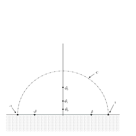
Figure 3.4: The contour for the non-trivial fixed point solution of the DWRG equation. It must run from $-1$ to $1$ going outside all bound state poles.

The construction of the perturbations around $\hat{V}_{S}^{(0)}$ follows in much the same way as in the Coulomb example,

$$\frac{1}{\hat{V}_{S}(\hat{p},\hat{\kappa},\Lambda)}=\frac{1}{\hat{V}_{S}^{(0)}(\hat{p},\hat{\kappa},\Lambda)}+\sum_{n,m_{i}=0}^{\infty}\hat{C}_{2n,m_{1},m_{2},\ldots}\left(\frac{\Lambda}{\Lambda_{0}}\right)^{2n+m_{1}+m_{2}+\ldots-1}{\hat{p}}^{2n}{\hat{\kappa}_{1}}^{m_{1}}{\hat{\kappa}_{2}}^{m_{2}}\ldots.$$ (3.97)

The LO perturbation is unstable as $\Lambda\rightarrow 0$, the NLO perturbations are marginal and correspond to the logarithmic counter terms. All other perturbations are stable as $\Lambda\rightarrow 0$. The power-counting scheme in the $\hat{\kappa}_{i}$-independent terms is precisely the KSW scheme. The RG flow is the same as described in the Coulomb example and the arguments about the usefulness of each power-counting scheme are the same.

The form for the basic loop integral 3.96 is extremely useful and will form the basis for non-trivial solutions in later chapters. The important property it possesses is that it is always analytic in the energy $\hat{p}$.

3.6.3 The DWERE and Interpretation of the Fixed Points

In all our examples, the physical interpretation of the trivial fixed point has, for want of a better word, been trivial. In the pure short range case the non-trivial fixed point corresponded to a system with a bound state at exactly threshold. Since we began our analysis of the DWRG we have used the non-trivial fixed point as a tool for constructing power-counting schemes and for understanding the RG flow but have failed to give an interpretation of it. To remedy this situation let us derive a DWERE by using the the non-trivial fixed point in this example. We substitute the potential into the equation for the $\tilde{T}$-matrix,

$$\frac{\langle\psi_{p}|\tilde{T}_{S}|\psi_{p}\rangle}{|\psi_{p}(R)|^{2}}=V_{S}(p,\kappa,\Lambda)\left(1-V_{S}(p,\kappa,\Lambda)\left[\frac{M}{2\pi^{2}}\int_{0}^{\Lambda}dq\frac{|\psi_{q}(R)|^{2}}{p^{2}-q^{2}+i\epsilon}+\frac{M}{4\pi}\sum_{n}\frac{|\psi_{n}(R)|^{2}}{p^{2}+p_{n}^{2}}\right]\right)^{-1}.$$ (3.98)

The term in square brackets on the right hand side may be written as

$$[\ldots]=\frac{M\Lambda R^{2}}{4i\pi^{2}}\left[\int_{-1}^{1}d\hat{q}\frac{\hat{q}}{\hat{p}^{2}-\hat{q}^{2}}\frac{f^{\prime}(\hat{q},0)}{{\cal F}(\hat{q},\hat{\kappa}_{i})}-2\pi i\,{\cal R}\left\{\frac{\hat{q}}{\hat{p}^{2}-\hat{q}^{2}+i\epsilon}\frac{f^{\prime}(\hat{q},0)}{{\cal F}(\hat{q},\hat{\kappa}_{i})},p\rightarrow ip_{n}\right\}\right],$$ (3.99)

where ${\cal R}\{f(z),z\rightarrow z_{0}\}$ indicates the residue of $f(z)$ at $z=z_{0}$. This result follows from definitions (3.83,3.90,3.94) and from the result for the normalisation of the bound states, (3.82). Inverting eqn. (3.98) and using the expression for the $\tilde{T}$-matrix in terms of the phaseshift correction we obtain after some algebra,

$$\frac{p}{|{\cal F}(p,\kappa_{i})|^{2}}(\cot\tilde{\delta}_{S}-i)+{\cal M}(p,\kappa_{i})=-\frac{2}{\pi\Lambda_{0}}\sum_{n,m_{i}=0}^{\infty}\hat{C}_{2n,m_{1},m_{2},\ldots}{\Lambda_{0}}^{-2n-m_{1}-m_{2}-\ldots}{p}^{2n}{\kappa_{1}}^{m_{1}}{\kappa_{2}}^{m_{2}}\ldots,$$ (3.100)

where ${\cal M}(\Lambda\hat{p},\Lambda\hat{\kappa}_{i})=\Lambda\hat{\cal M}(\hat{p},\hat{\kappa}_{i})$, we have absorbed any logarithmic counterterms into the marginal couplings and we have used the result:

$$\displaystyle{{\cal M}(p,\kappa_{i})=\frac{2\Lambda}{\pi}\Biggl{[}\frac{1}{2i}\int_{-1}^{1}d\hat{q}\frac{\hat{q}}{\hat{p}^{2}-\hat{q}^{2}+i\epsilon}\frac{f^{\prime}(\hat{q},0)}{{\cal F}(\hat{q},\hat{\kappa})}-\frac{1}{\hat{V}_{S}^{(0)}(\hat{p},\hat{\kappa})}}$$

$$\displaystyle{\qquad\qquad\qquad\qquad\qquad\qquad-\pi\,{\cal R}\left\{\frac{\hat{q}}{\hat{p}^{2}-\hat{q}^{2}}\frac{f^{\prime}(\hat{q},0)}{{\cal F}(\hat{q},\hat{\kappa}_{i})},p\rightarrow ip_{n}\right\}\Biggr{]},}$$ (3.101)

which follows from evaluating what is now a closed contour integral using Cauchy’s theorem, cancelling the bound state residues and evaluating the remaining residue at $\hat{q}=+\hat{p}$ (See Fig. 3.5). The final result is expressed as,

$$|{\cal F}(p,\kappa_{i})|^{-2}p(\cot\tilde{\delta}_{S}-i)+\frac{f^{\prime}(p,\kappa_{i},0)}{{\cal F}(p,\kappa_{i})}=-\frac{1}{\tilde{a}}+\frac{1}{2}\tilde{r}_{e}p^{2}+\ldots,$$ (3.102)

where the distorted wave scattering length and effective range may contain logarithmic dependence on some of the scales $\kappa_{i}$. Relationship (3.94) shows that the imaginary parts on the LHS cancel to ensure a real phaseshift, $\tilde{\delta}_{S}$.

The DWERE (3.102) has been derived before by van Haeringen and Kok [43], following the work of many others (see their references), in a somewhat more mathematically inspired manner. The advantage of this derivation is that, because of the EFT philosophy behind the derivation, we gain a physical rather than mathematical interpretation of how and when it may be used, i.e. when the series is likely to converge well.

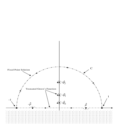
Figure 3.5: Evaluation of the removed non-analytic term in the general DWERE

To gain insight into the non-trivial fixed point let us examine what the DWERE looks like in the limit of all perturbations around the non-trivial fixed point going to zero. The DWERE when the solution is taken to be the non-trivial fixed point with no perturbations (i.e. $\tilde{a}\rightarrow\infty,\,\tilde{r}_{e}\rightarrow 0$ etc) can be written as:

$$\cot\tilde{\delta}_{S}=-\frac{1}{p}{\cal F}(p,\kappa_{i})f^{\prime}(-p,\kappa_{i},0)+i.$$ (3.103)

This may be re-written as an equation for $e^{2i\tilde{\delta}_{S}}$:

$$e^{2i\tilde{\delta}_{S}}=\frac{{\cal F}(-p,\kappa_{i})f^{\prime}(p,\kappa_{i},0)-2ip}{{\cal F}(-p,\kappa_{i})f^{\prime}(p,\kappa_{i},0)}=\frac{{\cal F}(p,\kappa_{i})f^{\prime}(-p,\kappa_{i},0)}{{\cal F}(-p,\kappa_{i})f^{\prime}(p,\kappa_{i},0)},$$ (3.104)

where the second identity follows from eqn. (3.91). When this is combined with the form for $e^{2i\delta_{L}}$, eqn. (3.80), we obtain an equation for the full $S$-matrix taking account of both long and short range physics,

$$e^{2i\delta}=e^{2i\delta_{L}}e^{2i\tilde{\delta}_{S}}=\frac{f^{\prime}(-p,\kappa_{i},0)}{f^{\prime}(p,\kappa_{i},0)}.$$ (3.105)

This equation leads to two interpretations of the non-trivial fixed point, one mathematical and the other physical.

Mathematically, to understand what this equation says let us look at the resulting wavefunctions, $\tilde{\psi}_{p}(r)$. Given the form of the $S$-matrix we know that at large $r$ the wavefunctions must go like

$$\tilde{\psi}_{p}(r)\rightarrow\frac{1}{2ip}\bigl{(}f^{\prime}(-p,\kappa_{i},0)e^{ipr}-f^{\prime}(p,\kappa_{i},0)e^{-ipr}\bigr{)}$$ (3.106)

and hence are given by (recalling that the short range force acts at zero radius, so that for $r>0$ the Schrödinger equation is unchanged from its long range counterpart),

$$\tilde{\psi}_{p}(r)=\frac{1}{2ip}\bigl{(}f^{\prime}(-p,\kappa_{i},0)f(p,\kappa_{i},r)-f^{\prime}(p,\kappa_{i},0)f(-p,\kappa_{i},r)\bigl{)}.$$ (3.107)

As $r\rightarrow 0$ these solutions satisfy the Neumann boundary condition, $\tilde{\psi}^{\prime}(p,\kappa_{i},r)=0$, rather than the usual Dirichlet boundary condition. This offers us a new interpretation of the trivial and non-trivial fixed points in terms of boundary conditions on the DWs. The trivial fixed point corresponds to the normal boundary condition of vanishing wavefunctions at $r=0$, while the non-trivial fixed point corresponds to the boundary condition of vanishing derivative at $r=0$.

The two solutions to the Schrödinger equation with these two different boundary conditions are linearly independent. Hence, the non-trivial fixed point changes each DW into a solution linearly independent to it and, in effect, changes it ‘by the maximum amount possible’. This interpretation of the non-trivial fixed point is also appropriate (as of course it should be) for the example in chapter $2$, in which there was no long range potential, and had been implicitly noted by van Kolck [10].

Physically, we can understand the non-trivial fixed point in terms of a bound state at zero energy. As $p\rightarrow 0$, $f^{\prime}(p,\kappa_{i},0)\rightarrow ip$, so that $e^{2i\delta}\rightarrow-1$ and $\delta(p=0)=(n+1/2)\pi$, which is the condition for a zero energy bound state. This interpretation is also in parallel with the pure short-range case.

3.6.4 Identification of Scales and the Yukawa Potential

One particular moot point where the Jost function DWRG analysis is important is in the inclusion of pions in an EFT for nucleons. We will now look at the issues surrounding the Yukawa potential and pions in an EFT for nucleons.

However, before we can discuss the physics of this problem, we must quickly tidy up one final mathematical issue. Our definition of $\hat{\cal M}$, eqn. (3.93), relies upon the existence of the limit of the derivative of the Jost function as $r\rightarrow 0$. This limit only exists for potentials that do not have a $r^{-1}$ divergence as $r\rightarrow 0$. For potentials that do diverge, such as the Yukawa potential, we must modify the definition of $\hat{\cal M}$. To understand the problem let us consider the expansion, in powers of $r$, of the Jost solution for the Yukawa potential for one pion exchange between nucleons of mass $M$. This potential is defined by,

$$MV_{L}(r)=2\kappa_{\pi}\frac{e^{-m_{\pi}r}}{r},$$ (3.108)

where,

$$\kappa_{\pi}=\frac{g_{A}^{2}m_{\pi}^{2}M}{32\pi f_{\pi}^{2}},$$ (3.109)

the inverse ‘pionic Bohr radius’ and $m_{\pi}$, the pion mass are the low energy scales associated with the potential. The Jost solution for the Yukawa potential is given by

$$f^{\pi}(p,\kappa_{\pi},m_{\pi},r)={\cal F}^{\pi}(p,\kappa_{\pi},m_{\pi})\left(1+{\cal M}_{\text{reg}}^{\pi}(p,\kappa_{\pi},m_{\pi})r+2\kappa_{\pi}r\ln m_{\pi}r+{\cal O}(r^{2})\right).$$ (3.110)

In this case the term $\sim r\ln m_{\pi}r$ means that the derivative of the Jost solution is not defined at $r=0$. However, inserting eqn. (3.110) into eqn. (3.91) shows that the identity (3.94) holds with $\hat{\cal M}^{\pi}_{\text{reg}}$ replacing $\hat{\cal M}$. The rest of the arguments for the non-trivial fixed point solution hold with the substitution $\hat{\cal M}$ replaced by $\hat{\cal M}^{\pi}_{\text{reg}}$ which we may write as

$$\hat{\cal M}_{\text{reg}}^{\pi}(\hat{q},\hat{\kappa}_{\pi},\hat{m}_{\pi})=\lim_{\hat{r}\rightarrow 0}\left[\frac{{f^{\pi}}^{\prime}(\hat{q},\hat{\kappa}_{\pi},\hat{m}_{\pi},\hat{r})}{{\cal F}^{\pi}(\hat{q},\hat{\kappa}_{\pi},\hat{m}_{\pi})}-2\hat{\kappa}_{\pi}\ln\hat{m}_{\pi}\hat{r}\right].$$ (3.111)

Without going into the details this results in a non-trivial fixed-point, $\hat{V}_{S}^{(0)}$, defined by eqn. (3.96) with logarithmic dependence on $\hat{m}_{\pi}$, which can be removed in the usual way. See refs. [44, 9, 45] for more details.

There has been some debate in the literature as to how to handle OPE in an EFT. One scheme (WvK) proposed by Weinberg [8] and further developed by van Kolck [49, 40], iterates it to all orders. Another, proposed by KSW [50], treats the force perturbatively.

So far in this section it has been understood that the long range potential has only low energy scales associated with it. In this case the analysis is simple and results in a choice of two expansions. A Weinberg scheme based upon the trivial fixed point and with terms in one-to-one correspondence with the terms in the DW Born expansion and a KSW scheme based upon the non-trivial fixed point and with terms in one-to-one correspondence with the terms in the DWERE. We shall see that it is the identification of the low-energy scales in the Yukawa potential that has led to such confusion.

Since the DWRG analysis promotes all low-energy physics to a fixed-point, if it was applied to the Yukawa potential with the two identified low energy scales $\kappa_{\pi}$ and $m_{\pi}$ it would be equivalent to the WvK scheme, summing the effects of one pion exchange to all orders and leaving a choice of power-counting schemes. For the strongly interacting nucleon system we would expect the non-trivial power-counting scheme and the DWERE to provide a parameterisation that converges up to the mass of the $\rho$-meson, $m_{\rho}=770$MeV [45]. This choice of low energy scales has resulted in some moderate success [49, 40].

Unfortunately there is an issue of debate. In the power-counting around the non-trivial fixed point, there are terms like

$$\frac{m_{\pi}^{2n}}{\Lambda_{0}^{2n-1}},$$ (3.112)

$$\frac{\kappa_{\pi}^{n}}{\Lambda_{0}^{n-1}}.$$ (3.113)

The first of these terms is proportional to $m_{\pi}^{2n}$ and occurs at order $d=2n-2$ in the power-counting. The second of these terms occurs at order $d=n-2$ in the power-counting, yet because $\kappa_{\pi}\propto m_{\pi}^{2}$ it is also proportional to $m_{\pi}^{2n}$. Hence, terms of the same order in $m_{\pi}$ occur at different orders in this power-counting and the direct link to ChPT has been lost [51, 50].

If we wish the nuclear EFT including OPE to be consistent with ChPT, then one solution is the KSW scheme [50]. In this case we treat the scale,

$$\Lambda_{NN}=\frac{16\pi f_{\pi}^{2}}{Mg_{A}^{2}}=300{\rm MeV},$$ (3.114)

as a high energy scale so that the Yukawa potential is given by

$$MV_{L}(r)=\frac{m_{\pi}^{2}}{\Lambda_{NN}}\frac{e^{-m_{\pi}r}}{r}$$ (3.115)

and occurs at the order $(Q/\Lambda_{0})^{1}$ in the EFT and so does not require summing to all orders. From the DWRG point of view, the effects of the Yukawa potential vanish as the cut-off $\Lambda\rightarrow 0$ and so do not get promoted into the fixed point. Thus the fixed points are the simple ones of the pure short range case. In this case the rescaled DW Green’s function $G_{L}$ can be expanded in powers of $\Lambda/\Lambda_{NN}$ and treated as perturbations around the non-trivial fixed point.

Unfortunately, despite consistency with ChPT, the resulting expansion turns out to be slowly convergent [45, 37, 38, 46] because of the small separation of scales between the pion mass, $m_{\pi}=140$MeV and $\Lambda_{NN}$.

Although the DWRG analysis gives the possible power-counting schemes that can be obtained from the non-trivial or trivial fixed point they can only ever be as good as the information put in. One must consider very carefully the scales in any particular problem.

3.7 Summary

In this chapter we have introduced the DWRG equation and solved it for several examples. The analysis for the Coulomb and general “well-behaved” potentials yielded known results that have both recently been used in EFTs. Despite these results being well-known, the method of derivation is novel and in itself is interesting. The conclusions regarding the usefulness of the two possible power-counting schemes are very much the same as arrived out for the pure short-range potential.

The method of solution of the DWRG fixed point equation in the final general example will prove extremely useful in later chapters and provides a robust way of solving these types of equation.

The other example considered in this chapter was the repulsive inverse square potential. As far as we are aware the results derived here are new. The power-counting schemes that are derived are novel and depend upon the strength of the potential. The conclusions about the use of either power-counting scheme are also different. If the inverse square potential is ‘strong’, the use of the non-trivial fixed point scheme may require the tuning of several parameters to unnaturally small values, something that may seem a little contrived. It is likely that in such a system the trivial fixed point should provide the correct power-counting scheme.

Chapter 4 The DWRG for Singular Inverse Square Potential

4.1 Introduction

The inverse square potential, eqn. (3.55) is an interesting example. When $\beta>-1/4$ the potential has a well-defined set of DWs. However, if $\beta<-1/4$ the potential becomes singular with no well-defined set of DWs. The reason for this is that any two linearly independent solutions of the Schrödinger equation cannot be resolved by a boundary condition at the origin. Indeed no solution of the Schrödinger equation has a well-defined value at the origin. Furthermore, it may appear at first glance that there is a continuum of possible bound states. The solution,

$$\psi\propto\sqrt{r}K_{i\nu}(\sqrt{-ME}r),$$ (4.1)

where $\nu=\sqrt{-1/4-\beta}$ and $K_{\mu}(z)$ is the modified Bessel function of the third kind, satisfies vanishing boundary conditions at infinity and the Schrödinger equation, yet the lack of a boundary condition at the origin means these bound states are not resolved into a discrete spectrum.

Mathematically, the problem with the potential is that the Hamiltonian is no longer self-adjoint [27, 28]. The solution is to make it so by introducing an extra boundary condition to uniquely define a solution [28, 29]. This extra boundary condition can be introduced in several ways, either by requiring vanishing wavefunctions at some radius, $R_{0}$, or by defining some bound state, $p_{0}$ [29]. However the boundary condition is defined it necessarily introduces a new scale into the problem. Mathematically, this is equivalent to forming a self-adjoint extension of the Hamiltonian [28, 27].

Once the self-adjoint extension is formed we have a complete set of DWs including a discrete spectrum of bound states, however there are still problems to be addressed. The resulting discrete spectrum consists of an infinite number of geometrically spaced bound states. These bound states accumulate at zero energy and have no ground state. The lack of a ground state shows that even after the self-adjoint extension is formed the full resolution of the short-range physics has not been achieved. Without a ground state the system would ‘implode’ radiating an infinite amount of energy.

The resolution of the attractive inverse square singularity in an EFT is critical to the understanding of the three-body KSW EFT [25, 22, 30, 24, 52, 65]. Several papers have attempted to resolve the problem by replacing the singularity with an ‘effective’ potential well at short range and then matching the logarithmic derivative of the wavefunctions in the two regions [31, 30, 32]. In each case the range, $R$, of the effective potential has been assumed to be far less than all inverse momenta. The matching criteria acts, in effect, as the boundary condition required to form the self-adjoint extension and does not, as correctly pointed out by Bawin and Coon [30] but not by Camblong and Ordóñez [31] give a ground state to the system. Further to this, using this method, the running of the ‘strength’ of the effective well is multi-valued [32].

The DWRG method provides the explanation to these problems. We find that the choice of a self-adjoint extension is equivalent to the LO EFT, which in turn corresponds to a marginal perturbation in the RG. Because the LO EFT is marginal it cannot distinguish between high and low energy states, which is why the self-adjoint extension cannot provide a ground state.

We shall also see that because of the lack of a ground state in the DWs, the DW Green’s function must be truncated in both the continuum and the bound states to obtain an unique solution to the DWRG. The multi-valuedness of the effective potential can then be attributed to different methods of truncating the bound states.

4.2 Defining the Distorted Waves

The distorted waves of the inverse square potential satisfy the Schrödinger equation,

$$\frac{{\rm d}^{2}}{{\rm d}r^{2}}\psi_{p}(r)-\frac{\beta}{r^{2}}\psi_{p}(r)+p^{2}\psi_{p}(r)=0,$$ (4.2)

of which the general solution can be written as a superposition of Bessel functions of order $\pm\sqrt{1/4+\beta}$. When $\beta<-1/4$ the orders of the Bessel functions are imaginary and the general solution is,

$$\psi_{p}(r)=\sqrt{r}(A_{1}J_{i\nu}(pr)+A_{2}J_{-i\nu}(pr)),$$ (4.3)

where $\nu=\sqrt{-\beta-1/4}$. It is impossible to find a unique solution by defining a boundary condition at the origin. To resolve the ambiguity and form a self-adjoint extension we begin by considering the Jost solution $f(p;r)$ that satisfy the Schrödinger equation and has the unambiguous asymptotic boundary condition, $f(p;r)\rightarrow e^{ipr}$ as $r\rightarrow\infty$. $f$ is easily found to be

$$f(p;r)=\sqrt{\frac{\pi pr}{2}}e^{-\frac{\pi}{4}(2\nu-i)}H^{(1)}_{i\nu}(pr),$$ (4.4)

where $H^{(1)}_{\mu}(z)$ is the Hankel function of the first kind. We would now like to define a Jost function, $\cal F$ in terms of the value of the Jost solution, $f$, at the origin but this limit does not exist. Explicitly, in the limit of $r\ll 1/p$ we have,

$$\sqrt{\frac{2}{\pi pr}}f(p;r)\sim\sin\left(\nu\log\frac{pr}{2}-\theta-i\frac{\pi\nu}{2}\right),$$ (4.5)

where $\theta=\arg\{\Gamma(1+i\nu)\}$. The solution is to define the Jost function in terms of the value of the Jost solution at the point $r=R_{0}$ rather than at $r=0$, resulting in,

$${\mathcal{F}}(p)=\frac{2e^{-\frac{i\pi}{4}}}{\sqrt{\pi\nu\sinh(\pi\nu)}}\sin\left(\eta(p)+i\frac{\pi\nu}{2}\right),$$ (4.6)

where

$$\eta(p)=-\nu\ln{\frac{pR_{0}}{2}}+\theta=-\nu\ln{\frac{p}{p_{0}}}.$$ (4.7)

Eqn. (4.7) defines the scale $p_{0}$, which as we shall see is simply related to the binding energies of the bound states. The definition of the Jost function introduced here is equivalent to applying a boundary condition of vanishing wavefunctions at the small distance $r=R_{0}$. With these definitions, the free DWs are given precisely as in eqn. (3.79), from which follows the usual relation between the $S$-matrix and the Jost function,

$$e^{2i\delta_{L}(p)}=\frac{{\mathcal{F}}(-p)}{{\mathcal{F}}(p)}=i\frac{\sin(\eta(p)-i\pi\nu/2)}{\sin(\eta(p)+i\pi\nu/2)}.$$ (4.8)

With the Jost function we may begin to investigate the bound states. The eigenvalues, $-p_{n}^{2}$, of the Hamiltonian are given by the poles of the $S$-matrix or equivalently the zeros of the Jost function. Using the definition of ${\mathcal{F}}(p)$ and $\eta(p)$ we find that these zeroes are defined by,

$$p_{n}=p_{0}\exp{\left(\frac{n\pi}{\nu}\right)}\qquad n\in{\mathbb{Z}}.$$ (4.9)

Thus, these bound states, $\psi_{n}(r)$, form an infinite tower of states with geometrically spaced energies. It is clear that a ground state does not exist and that the states get infinitesimally close to zero energy. Since the distorted waves now form a complete set, the familiar spectral decomposition of the Green’s function follows. The Green’s function with standing wave boundary conditions is given by,

$$G_{L}(p;r,r^{\prime})=\frac{M}{2\pi^{2}}\fint_{0}^{\infty}{\rm d}q\frac{\psi_{q}(r)\psi_{q}(r^{\prime})}{p^{2}-q^{2}}+\frac{M}{4\pi}\sum_{n=-\infty}^{\infty}\frac{\psi_{n}(r)\psi_{n}(r^{\prime})}{p^{2}+p_{n}^{2}}.$$ (4.10)

Explicitly the DWs, given by eqn. (3.79), are

$$\psi_{p}(r)=\sqrt{\frac{\pi pr}{2}}\frac{1}{2i|\sin(\eta(p)+i\pi\nu/2)|}\Bigl{(}e^{i\eta(p)}J_{i\nu}(pr)-e^{-i\eta(p)}J_{-i\nu}(pr)\Bigr{)},$$ (4.11)

and the bound states are,

$$\psi_{n}(r)=\sqrt{\frac{2r\sinh{(\pi\nu)}}{\pi\nu}}p_{n}K_{i\nu}(p_{n}r).$$ (4.12)

The definition of the Jost function in terms of the Jost solution at $r=R_{0}$ provides the additional boundary condition, which in turn forms a self-adjoint extension of the Hamiltonian. However, in obtaining the Jost function in this way we have implicitly assumed $R_{0}\ll 1/k$ for all $k$, i.e. $R_{0}$ is some infinitesimal distance, which makes it difficult to understand the exact nature of the boundary condition. Fortunately, this method lends itself to different interpretations. Firstly, and perhaps most simply, $R_{0}$ fixes the phase of the trig-log behaviour close to the origin and hence defines a regular and irregular solution. Secondly, $p_{0}$ acts as a choice of a particular bound state, which forces all other bound states to fall into the exponential tower defined by eqn. (4.9). Importantly this means that the relationship between $p_{0}$ and choice of self-extension is not one-to-one. Any choice given by $p^{\prime}_{0}=p_{0}e^{n\pi/\nu}$ is equivalent to the choice $p_{0}$.

4.3 The DWRG equation

We now move on to the construction and solution of the DWRG equation for the short range force. Now that we have arrived at an equivalent of the Jost function for the attractive inverse square potential it may be hoped that the general analysis used in section 3.6 will yield a method of solving the DWRG equation. However, we are immediately faced with a problem. In the previous analysis the contour of integration in eqn. (3.95) for the DWRG basic loop integral solution had to go outside all the bound state poles to avoid being ‘pinched’ as the scales associated with the long range potential went to zero, in this case it is quite impossible for the contour to go outside all of the bound state poles because there is no ground state.

With a little thought, our inability to define a contour that goes outside the bound state poles is not a problem. The position of the poles is controlled by the self-adjoint extension defining scale, $p_{0}$. As long as we are not concerned with analyticity of the short-range force as $p_{0}\rightarrow 0$ then there is no worry with being pinched as $p_{0}\rightarrow 0$.

With this problem resolved a new one becomes apparent, namely non-unique solutions to the DWRG equation. To explain, if we are to define our basic loop integral solution in a method like that outlined in section 3.6 our contour of integration must cross the imaginary axis between two particular poles, with no apparent correct choice of which two poles. Without resolving this issue, any resulting physical observables will invariably depend upon the choice of contour.

It is clear that this problem is a result of the lack of a ground state which in turn is a result of the singular behaviour of the long-range potential close to the origin. The philosophy behind the DWRG is to ‘replace’ all the interactions between high energy distorted waves with an effective short-range interaction, it therefore makes sense that the deeply bound states, which are a result of the inverse square singularity, should be cut-off. Thus, we define the truncated Green’s function to be,

$$G_{L}(p,\Lambda;r,r^{\prime})=\frac{M}{2\pi^{2}}\fint_{0}^{\Lambda}{\rm d}q\frac{\psi_{q}(r)\psi_{q}(r^{\prime})}{p^{2}-q^{2}}+\frac{M}{4\pi}\sum_{|p_{n}|<\Lambda}\frac{\psi_{n}(r)\psi_{n}(r^{\prime})}{p^{2}+p_{n}^{2}},$$ (4.13)

in which all distorted waves with energies outside the range $(-\Lambda^{2}/M,\Lambda^{2}/M)$ are removed. As we shall see the truncation of bound states and subsequent renormalisation specifies a non-trivial fixed point solution and leads to well-defined results for physical observables. The method of truncating the bound states chosen here is far from unique, other truncation methods will specify different solutions, however because of the renormalisation procedure, physical observables will be independent of the truncation method and of the specific loop integral.

The differential equation, (3.21), for $V_{S}$ is now given by,

$$\frac{\partial V_{S}}{\partial\Lambda}=-\frac{M}{2\pi^{2}}V_{S}^{2}\left[\frac{|\psi_{\Lambda}(R)|^{2}}{p^{2}-\Lambda^{2}}+\frac{\pi}{2}\sum_{n=-\infty}^{\infty}\frac{|\psi_{n}(R)|^{2}}{p^{2}+p_{n}^{2}}\delta(\Lambda-p_{n})\right],$$ (4.14)

where the cutting off of bound states has resulted in a series of discontinuities expressed in terms of a sum of delta functions. Since $R$ is taken as very small, the distorted waves go to,

$$|\psi_{\Lambda}(R)|^{2}\rightarrow\frac{\Lambda B(R)\sinh{\pi\nu}}{\cosh{\pi\nu}-\cos{2\eta(\Lambda)}},\qquad|\psi_{n}(R)|^{2}\rightarrow\frac{2p_{n}^{2}}{\nu}B(R),$$ (4.15)

where

$$B(R)=\frac{R}{\nu}\sin^{2}\left(\nu\ln\left(\frac{p_{0}R}{2}\right)-\theta\right).$$ (4.16)

The final step to obtain the DWRG equation is to rescale. In this problem, the only low energy scale is the on-shell momentum, $p$, which is rescaled to $\hat{p}=p/\Lambda$. $V_{S}$ is rescaled by the relation,

$$\hat{V}_{S}(\hat{p},\Lambda)=\frac{MB(R)}{2\pi^{2}}V_{S}(\hat{p}\Lambda,\Lambda),$$ (4.17)

finally resulting in the DWRG equation,

$$\displaystyle{\Lambda\frac{\partial}{\partial\Lambda}\left(\frac{1}{\hat{V}_{S}}\right)=\hat{p}\frac{\partial}{\partial\hat{p}}\left(\frac{1}{\hat{V}_{S}}\right)-\frac{\sinh{\pi\nu}}{(\cosh{\pi\nu}-\cos{2\nu\ln(\Lambda/p_{0})})(1-\hat{p}^{2})}}$$

$$\displaystyle{\qquad\qquad\qquad+\frac{\pi}{\nu}\sum_{n=-\infty}^{\infty}\frac{1}{\hat{p}^{2}+1}\Lambda\delta(\Lambda-p_{n}),}$$ (4.18)

where we have divided through by $\hat{V}_{S}^{2}$ to obtain a linear equation in $1/\hat{V}_{S}$. Unlike all the RG equations seen so far this one has $\Lambda$ dependence in the inhomogeneous term on the RHS. This dependence is a result of the scale $p_{0}$, which may not be treated as a low energy scale.

4.4 Solving the DWRG equation

The DWRG equation, as always, yields a trivial fixed point, $\hat{V}_{S}=0$. The perturbations, $\hat{V}_{S}=C\Lambda^{\nu}\phi_{\nu}(\hat{p})$, satisfy the equation

$$\phi^{\prime}_{\nu}(\hat{p})=\nu\phi_{\nu}(\hat{p}).$$ (4.19)

We find $\phi_{\nu}(\hat{p})=\hat{p}^{\nu}$. The corresponding RG eigenvalues are $\nu=0,2,4,\ldots$. Hence, the RG solution in the region of the trivial fixed point is given by,

$$\hat{V}_{S}(\Lambda,\hat{p})=\sum_{n=0}^{\infty}\hat{C}_{2n}\left(\frac{\Lambda}{\Lambda_{0}}\right)^{2n}\hat{p}^{2n}.$$ (4.20)

The LO term is marginal, i.e. it does not scale with any power of $\Lambda$ and is expected to be associated with some logarithmic behaviour in $\Lambda$. However, before we can give a full explanation of this we must obtain the full solution to the RG equation.

It is clear, because of the $\Lambda$-dependence on the right-hand side of equation (4.3), that no other fixed point solution can be found. However, since that dependence is only logarithmic we may hope to find a slowly evolving solution. (Such a solution will be no worse than that encountered when considering the Coulomb potential, in which logarithmic dependence on $\Lambda$ was introduced to remove logarithmic dependence upon $\hat{\kappa}$.) A logarithmically evolving fixed point solution may still be used to construct a power-counting by perturbing about it in powers of $\Lambda$.

Since (c.f eqn. (3.94)),

$$\frac{\sinh{\pi\nu}}{\cosh{\pi\nu}-\cos{2\nu\ln{\Lambda/p_{0}}}}=\frac{1}{2i}\left[\cot\left(\nu\ln\frac{\Lambda}{p_{0}}-\frac{i\pi\nu}{2}\right)-\cot\left(\nu\ln\frac{\Lambda}{p_{0}}+\frac{i\pi\nu}{2}\right)\right],$$ (4.21)

we can immediately write down a solution to the continuous part of the DWRG equation in parallel to eqn. (3.95) considered in section 3.6:

$$\frac{1}{\hat{V}_{S}^{(0)}(\hat{p},\Lambda)}=\frac{1}{2i}\int_{C}d\hat{q}\frac{\hat{q}}{\hat{p}^{2}-\hat{q}^{2}}\cot\left(\nu\ln\frac{\hat{q}\Lambda}{p_{0}}-\frac{i\pi\nu}{2}\right),$$ (4.22)

which is clearly analytic as $\hat{p}\rightarrow 0$. The contour $C$ is shown in Fig. 4.1, it follows a path from $\hat{q}=-1$ to $\hat{q}=1$. The position of bound state poles poles shown in Fig. 4.1 are simply given by,

$$i\hat{p}_{n}=i\frac{p_{n}}{\Lambda}=i\frac{p_{0}}{\Lambda}e^{n\pi/\nu}.$$ (4.23)

The position of these poles varies with $\Lambda$. This is in contrast to the examples considered so far where the rescaling of the scales in the long-range potential meant that the bound state poles in the complex $\hat{q}$-plane were independent of $\Lambda$ (which of course is what one would hope if looking for a fixed point solution). The poles in this example move up the imaginary $\hat{q}$ axis as $\Lambda\rightarrow 0$ because the scale that initially controlled their positions, $p_{0}$, is treated as a high energy scale and not absorbed into the fixed-point solution.

Figure 4.1: The contour in the complex $\hat{q}$-plane for the non-trivial fixed point solution of the DWRG equation. It runs from $-1$ to $1$ and crosses the imaginary axis at $\hat{q}=i$. The bound state poles occur at $\hat{q}=i\hat{p}_{n}=ip_{0}e^{n\pi/\nu}/\Lambda$.

Fortunately this migration of the bound state poles with $\Lambda$ is to our benefit as it enables us to create the necessary discontinuities in the DWRG solution by allowing the bound state poles to cross the contour of integration. Dividing eqn. (4.3) through by $\Lambda$ and integrating it with respect to $\Lambda$ from $p_{n}-\epsilon$ to $p_{n}+\epsilon$ we get the discontinuity at $\Lambda=p_{n}$,

$$\left[\frac{1}{\hat{V}_{S}}\right]_{\Lambda=p_{n}-\epsilon}^{\Lambda=p_{n}+\epsilon}=\frac{\pi}{\nu}\frac{1}{\hat{p}^{2}+1}.$$ (4.24)

If we chose the contour $C$ so that it crosses the imaginary axis at the point $\hat{q}=i$ then from eqn. (4.23) it follows that the bound state pole at $\hat{q}=i\hat{p}_{n}$ crosses the contour of integration when $\Lambda=p_{n}$ and produces the correct discontinuity, namely

$$\left[\frac{1}{\hat{V}_{S}}\right]_{\Lambda=p_{n}-\epsilon}^{\Lambda=p_{n}+\epsilon}=-2\pi i{\cal R}\left\{\frac{1}{2i}\frac{\hat{q}}{\hat{p}^{2}-\hat{q}^{2}}\cot\left(\nu\ln{\hat{q}}-\frac{i\pi\nu}{2}\right),\hat{q}\rightarrow i\right\}=\frac{\pi}{\nu}\frac{1}{\hat{p}^{2}+1}.$$ (4.25)

Hence, $\hat{V}_{S}^{(0)}$ is a “fixed point” solution to the DWRG. From its definition it is readily observed that $\hat{V}_{S}^{(0)}$ is invariant under the transformation $\Lambda\rightarrow\Lambda e^{n\pi/\nu}$ so that $\hat{V}_{S}^{(0)}$ has log-periodic behaviour in $\Lambda$. Rather than use the rather stretched notation of a fixed point we shall, more appropriately refer to it as a limit cycle solution.

The explicit demonstration of limit-cycle behaviour in the RG for this problem confirms what has been shown at LO in several articles [32, 22, 24]. The first example of a RG limit cycle solution was given by Wilson and Glazek [53] in a toy model. Since then, because of its importance in the three-body EFT, many authors have taken an interest in such solutions [54, 32, 30, 55, 65].

Perturbations around this limit cycle are obtained in the usual way. In fact the eigenvalue equation for the perturbation is exactly the same as that for the trivial fixed point, (4.19) with the same result. Because the DWRG equation (4.3) for $\hat{V}_{S}^{-1}$ is linear, these perturbations give an exact solution to the RG equation,

$$\frac{1}{\hat{V}_{S}(\hat{p},\Lambda)}=\frac{1}{\hat{V}_{S}^{(0)}(\hat{p},\Lambda)}+\sum_{n=0}^{\infty}\hat{C}_{2n}\left(\frac{\Lambda}{\Lambda_{0}}\right)^{2n}\hat{p}^{2n}.$$ (4.26)

The LO term is marginal and is associated with the logarithmic flow in the limit cycle solution. Since there is a marginal (or $\Lambda$-independent) perturbation, it cannot be unambiguously removed from any limit cycle solution. This means that there is, in fact, a family of limit cycle solutions parameterised by the value of the marginal perturbation $\hat{C}_{0}$.

Previous examples of logarithmic behaviour in the scale $\Lambda$ resulted from a need to remove logarithmic behaviour in some low-energy scale and necessitated the introduction of an arbitrary scale, $\mu$. In this example however, no new scale needs to be introduced since the scale $p_{0}$ fills its purpose.

Where an arbitrary scale was introduced previously it could be traded off against the marginal perturbation leaving one remaining degree of freedom. It is not clear that $p_{0}$ and $\hat{C}_{0}$ represent the same degree of freedom, resolution of this issue must wait until we consider the effects of the long and short range potentials in tandem as $p_{0}$ also effects the long-range physics.

The RG flow is illustrated in Figs. 4.2 and 4.3. These diagrams show the flow of solutions $\hat{V}_{S}$ with $\Lambda$. Fig. 4.2 shows the running of $\hat{V}_{S}^{(0)}(\hat{p}\rightarrow 0,\Lambda)^{-1}$. The bold line shows the solution $1/\hat{V}_{S}^{(0)}$, the dotted lines show the discontinuities. The solution follows a logarithmically evolving cycle with discontinuities as each bound state is cut-off. Any member of the family of limit cycle solutions can be obtained by adding a marginal term, $\hat{C}_{0}$. In Fig. 4.2 this would simply appear as a constant shift up or down without change in form or period. From this diagram alone it is clear that $\hat{C}_{0}$ and $p_{0}$ cannot represent the same degree of freedom in the limit-cycle solution because variation of $p_{0}$ will produce a horizontal rather than vertical shift in the form of $1/\hat{V}_{S}^{(0)}$.

The limit-cycle behaviour is illustrated in fig. 4.3, which shows the RG flow in the familiar slice through the space $(b_{0}(\Lambda),b_{2}(\Lambda),\ldots)$. Again the solution $\hat{V}_{S}^{(0)}$ is shown in bold. The dashed lines show general solutions generated by perturbing with $\hat{C}_{2}$. The solution $\hat{V}_{S}^{(0)}$ acts as a limit-cycle solution that loops at a logarithmic rate in $\Lambda$ with a discontinuity as each bound state is cut-off . All more general solutions move in a cycle (with discontinuities) that tends to $\hat{V}_{S}^{(0)}$ like $\Lambda^{2}$ as $\Lambda\rightarrow 0$.

Figure 4.2: The running of $1/\hat{V}_{S}(0,\Lambda)$ with $\Lambda$ for $\nu=0.3$. The dotted lines show discontinuities.

Figure 4.3: The flow of $\hat{V}_{S}(\hat{p},\Lambda)=\sum b_{2n}(\Lambda)\hat{p}^{2n}$ with $\Lambda$ of $V_{S}^{(0)}$ (bold line) and stable perturbations about that (dashed lines). The dotted lines show discontinuities.

Having obtained a general solution to the DWRG we may now understand the nature of the trivial fixed point. As $\hat{C}_{0}\rightarrow\infty$ in eqn. (4.26), the general solution $\hat{V}_{S}\rightarrow 0$, i.e the limit cycle solution converges on the trivial fixed point. This means that the trivial fixed point is a special case of the more general family of limit-cycle solutions, in which the whole limit-cycle has been compacted into a point. If the RG flow is perturbed away from the trivial fixed point with a marginal term it moves into a nearby limit cycle.

The nature of the renormalisation group flow means that no particular tuning of the parameter $\hat{C}_{0}$ is required. Its exact value merely specifies which limit cycle the RG flow will converge upon. As we shall see each of these different limit cycles corresponds to a different ‘shift’ in the self-adjoint phase $\eta$ and that there is a one-to-one relationship between all possible limit-cycles and all possible self-adjoint extensions.

4.5 Full $S$-matrix and bound states

Using very much the same procedure that yields the distorted wave effective range expansion in section 3.6 we may write an expression for the correction to the phaseshift $\tilde{\delta}_{S}$ as,

$$\sinh{\pi\nu}\cot{\tilde{\delta}_{S}}=\sin{2\eta(p)}-\frac{2}{\pi}\bigl{(}\cosh{\pi\nu}-\cos 2\eta(p)\bigr{)}\sum_{n=0}^{\infty}\hat{C}_{2n}\left(\frac{p}{\Lambda_{0}}\right)^{2n}.$$ (4.27)

Equation (4.27) still leaves the relation between the marginal perturbation and the scale $p_{0}$ clouded. Since $p_{0}$ also appears in the equation for the long-range component of the phaseshift, $\delta_{L}$, the relationship between $p_{0}$ and $\hat{C}_{0}$ may become more transparent in consideration of the full $S$-matrix. Study of the full $S$-matrix may also highlight the significance of the RG solution $\hat{V}_{S}^{(0)}$ and make examination of the bound states possible. The full $S$-matrix is obtained from equations (4.8) and (4.27),

$$e^{2i\delta}=i\frac{\bar{Z}^{*}(p)}{\bar{Z}(p)},\qquad\bar{Z}(p)=\cos\left(\eta(p)+\frac{i\pi\nu}{2}\right)-\frac{2}{\pi}\sin\left(\eta(p)+\frac{i\pi\nu}{2}\right)\sum_{n=0}^{\infty}\hat{C}_{2n}\left(\frac{p}{\Lambda_{0}}\right)^{2n}.$$ (4.28)

In the limit of all perturbations, $\hat{C}_{2n}$, going to zero (or equivalently the RG solution reducing to $\hat{V}_{S}^{(0)}$) we have,

$$\bar{Z}(p)\rightarrow\cos\left(\eta(p)+\frac{i\pi\nu}{2}\right).$$ (4.29)

Comparing this to equation (4.8) for the pure long-range force, we see that there has been a maximal change in the arbitrary phase $\eta$. The effect of the solution $\hat{V}_{S}^{(0)}$ is to move the choice of self-adjoint extension, made in constructing the distorted waves, by a factor $\pi/2$. The significance of the $\hat{V}_{S}^{(0)}$ is now resolved, it is the solution to the RG equation that is‘furthest away’, in the sense of maximum possible change of physical observables, from the trivial solution $\hat{V}_{S}=0$, which of course would leave the full $S$-matrix unchanged from (4.8). This interpretation is very much in parallel to that arrived at in the previous chapter for the non-trivial fixed point for well-behaved potentials. In general we may say that the non-trivial fixed point solution changes the boundary condition that defines the regular solution to its linearly independent boundary condition.

Physically one may interpret the limit cycle $\hat{V}_{S}^{(0)}$ in terms of its action on the bound states, which are shifted to the geometric mean of the original set of states.

The existence of the marginal eigenvalue, $\hat{C}_{0}$, and the scale $p_{0}$ leads to an embarrassment of parameters that may be resolved if it is apparent that they do in fact represent the same degree of freedom in the effective theory. This freedom is not manifest in equation (4.28) but with the correct rewriting of the parameters, $\hat{C}_{2n}$,

$$\hat{C}_{0}=-\frac{\pi}{2}\cot\sigma,\qquad\frac{2}{\pi}\sum_{n=1}^{\infty}\hat{C}_{2n}\left(\frac{p}{\Lambda_{0}}\right)^{2n}=\frac{\csc\sigma\sum_{n=1}^{\infty}\hat{C}^{\prime}_{2n}\left(\frac{p}{\Lambda_{0}}\right)^{2n}}{\sin\sigma+\cos\sigma\sum_{n=1}^{\infty}\hat{C}^{\prime}_{2n}\left(\frac{p}{\Lambda_{0}}\right)^{2n}},$$ (4.30)

in terms of the new parameters, $\sigma$ and $\hat{C}^{\prime}_{2n}\,,n\geq 2$ we are left with a far more transparent parameterisation,

$$e^{2i\delta}=i\frac{Z^{*}(p)}{Z(p)},\qquad Z(p)=\sin\left(\eta(p)+\sigma+\frac{i\pi\nu}{2}\right)+\cos\left(\eta(p)+\sigma+\frac{i\pi\nu}{2}\right)\sum_{n=1}^{\infty}\hat{C}^{\prime}_{2n}\left(\frac{p}{\Lambda_{0}}\right)^{2n}.$$ (4.31)

Recalling that $\eta(p)=-\nu\ln(p/p_{0})$, eqn. (4.31) for the $S$-matrix clearly shows the overlapping roles of $\hat{C}_{0}$ and $p_{0}$. The scale $p_{0}$ acted originally to define a self-adjoint extension, through the marginal term in the short range force we may change it to any other choice of self-adjoint extension.

The space of all limit-cycle solutions is mapped out as $\hat{C}_{0}$ varies from $-\infty$ to $\infty$ or, from eqn. (4.30), as $\sigma$ varies from $0$ to $\pi$. In turn the variation of $\sigma$ from $0$ to $\pi$ with $p_{0}$ fixed maps out all possible self-adjoint extensions. Hence, the relationship between possible limit-cycle solutions of the DWRG equation and self-adjoint extensions is one-to-one. This is in stark contrast to the relationship between choices of $p_{0}$ and self-adjoint extensions where many equivalent $p_{0}$’s existed. In practice, we may ignore the phase $\sigma$ and allow the self-adjoint extension to be defined by our original choice, $p_{0}$.

The EFT bound states are given by the zeros of $Z(p)$. The position of the shallower bound states are virtually unmodified from the original theory and are controlled by the scale $p_{0}$ with minimal dependence upon $\hat{C}_{2n}$. There is of course still an accumulation of bound states at zero energy, though this is expected as these states exist because of the inverse square tail of the potential, which is unaffected by the short-range forces. The deepest states within the validity of the EFT, $p<\Lambda_{0}$, are strongly affected by the higher order perturbations. Beyond the range of validity, $p>\Lambda_{0}$, we can say nothing about the bound states except that some other physics must come into play to ensure that a ground state exists.

4.6 Truncation of Bound states and Uniqueness of Solutions.

Questions still remain about the the truncation of the bound states. It is obvious that some sort of regularisation of these states is necessary, yet the method of truncation of the bound states chosen above, though convenient and intuitive, is rather arbitrary. However, with a little thought it is quite straightforward to show that no matter how the bound state truncation is performed, a solution to the RG equation similar to that found above can be found and that more importantly the physical results will be identical.

For example, suppose we choose to truncate the bound states with a second cut-off $\mu$. Then the renormalisation prescription states that physical variables should be independent of $\mu$ as well as $\Lambda$. The DWRG equation will be the same as (4.3) without the $\delta$-function terms. It can be solved in a similar way to the discontinuous DWRG equation,

$$\frac{1}{\hat{V}_{S}^{(0)}(\hat{p},\Lambda,\mu)}=\frac{1}{2i}\int_{C(\Lambda,\mu)}d\hat{q}\frac{\hat{q}}{\hat{p}^{2}-\hat{q}^{2}}\cot\left(\nu\ln\frac{\Lambda\hat{q}}{p_{0}}-\frac{i\pi\nu}{2}\right),$$ (4.32)

where the contour $C(\Lambda,\mu)$ still runs from $1$ to $-1$ but now follows a $\Lambda$-dependent path that ensures that as $\Lambda$ varies no bound state poles cross it. The exact path of the contour (i.e. which two bound state poles it passes between) is then uniquely specified by the renormalisation condition on $\mu$. The solution to this DWRG equation is of course quite arbitrary without the second renormalisation condition.

Figure 4.4: The discontinuous solution $1/\hat{V}_{S}^{(0)}$ and the family of continuous solutions that result from an alternative method of truncation of the bound states ($\nu=0.3$).

The family of solutions that result are illustrated in Fig.4.4, which shows the previous discontinuous solution, $1/\hat{V}_{S}^{(0)}$, in bold with the discontinuities dotted and the various continuous solutions as dashed lines. Which solution is correct depends on $\mu$. Notice, that the correspondence between $\mu$ and the continuous RG solutions is not bijective; any two values of $\mu$ between $|p_{n}|$ and $|p_{n+1}|$ will map to the same continuous solution. More generally any prescription for truncating bound states will give a unique RG solution, jumping to the next branch of the solutions as a bound state is cut-off.

4.7 Summary

In this section we have looked at the attractive inverse square potential and the use of the DWRG equation in resolving its singular behaviour. The first step was to introduce a self-adjoint extension to the Hamiltonian by defining a Jost function. This allows definition of the DWs but does not resolve the singular behaviour. In particular, even after definition of a self-adjoint extension there is no ground state.

In order to produce a unique result for the EFT $S$-matrix it was necessary to truncate the deeply bound states that are a result of the singular behaviour of the long range potential. The basic loop integral solutions to the DWRG take the form of limit cycles towards which all more general solutions tend as $\Lambda\rightarrow 0$.

The limit cycle solutions are associated with a marginal perturbation in the DWRG. The degree of freedom embodied in this perturbation is the same as that in the choice of self-adjoint extension. Despite the complications in obtaining it, the EFT $S$-matrix, (4.31), takes a satisfyingly simple form.

It is difficult to link the limit cycle behaviour seen in our approach to the those seen by Bawin and Coon [30] and by Beane et al [32]. Their methods rely upon constructing a self-adjoint extension and short-range force in one step rather than the two step process that our method requires. So whereas their LO force defines the self-adjoint extension ours serves to change the original choice. What is particularly pleasing is the common approach of this chapter and section 3.6. The limit-cycle solutions do not require any particular special treatment apart from the truncation of bound states to specify the ‘branch’ of the multi-valued solution.

The truncation of bound states in this problem is forced upon us in seeking unique physical results. It resolves many of the issues raised about multi-valued solutions to the RG in refs. [30, 32]. The need to truncate bound states in this problem occurs because their position is controlled by a scale, $p_{0}$, that cannot be rescaled and absorbed into the limit-cycle.

Chapter 5 The DWRG for Three-Body Forces

In this chapter we shall consider the DWRG equation for three body forces (3BDWRG). In particular we shall derive the 3BDWRG equation for a general system for which the two-body forces are known but the three-body force is to be constructed using the 3BDWRG. The equation is applied to a system in which the pairwise forces are “well-behaved” in the sense of section 3.6 and then, more interestingly, used to examine the power-counting for the three body force in the KSW EFT for short range forces.

5.1 The Faddeev Equations and the Three-Body Force.

For a system with three particles the LS equation is inadequate. Although the three-body $T$-matrix satisfies the LS equation, it is not possible to use this equation to find it because its kernel is not compact. This is because a single LS equation is not enough to specify all the boundary conditions for a three-body DW. The solution is to use the Faddeev equations (see Appendix C).

Consider the case of three identical bosons interacting via a pairwise interaction $V_{2B}$. The wavefunction is written as

$$|\Psi^{+}\rangle=|\psi_{0}\rangle+(1+P)|\psi^{+}\rangle,$$ (5.1)

where $|\psi_{0}\rangle$ is the ‘in’-state and solves the free Schrödinger equation and $P$ is a permutation operator, which permutes particle indices and has the matrix elements

$$\displaystyle{\langle{\bf x}_{12},{{\bf y}}_{3}|P|{\bf x}_{12}^{\prime},{\bf y}_{3}^{\prime}\rangle=\delta^{3}({\bf x}_{12}-{\bf x}_{23}^{\prime})\delta^{3}({\bf y}_{3}-{\bf y}_{1}^{\prime})+\delta^{3}({\bf x}_{12}-{\bf x}_{31}^{\prime})\delta^{3}({\bf y}_{3}-{\bf y}_{2}^{\prime})}$$

$$\displaystyle{\qquad\qquad=\delta^{3}\left({\bf x}_{12}+\frac{1}{2}{\bf x}_{12}^{\prime}+{\bf y}_{3}^{\prime}\right)\delta^{3}\left({\bf y}_{3}-\frac{3}{4}{\bf x}_{12}^{\prime}+\frac{1}{2}{\bf y}_{3}^{\prime}\right)}$$

$$\displaystyle{\qquad\qquad\qquad+\delta^{3}\left({\bf x}_{12}+\frac{1}{2}{\bf x}_{12}^{\prime}-{\bf y}_{3}^{\prime}\right)\delta^{3}\left({\bf y}_{3}+\frac{3}{4}{\bf x}_{12}^{\prime}+\frac{1}{2}{\bf y}_{3}^{\prime}\right)}.$$ (5.3)

The Faddeev equation for the wavefunction is written as,

$$|\psi^{+}\rangle=G_{0}^{+}(p)t^{+}(p)|\psi_{0}\rangle+G_{0}^{+}(p)t^{+}(p)P|\psi^{+}\rangle,$$ (5.4)

where $t^{+}$ is the $T$-matrix given by the equation, $t^{+}(p)=V_{2B}+V_{2B}G_{0}^{+}(p)t^{+}(p)$. The corresponding equations for the full three-body Green’s function and $T$-matrix now follow from similar decompositions. If we write the full $T$-matrix, $\cal T$, in terms of components,

$${\cal T^{+}}(p)=(1+P)T^{+}(p),$$ (5.5)

then the Faddeev equation for the $T$-matrix component is,

$$T^{+}(p)=t^{+}(p)+t^{+}(p)G_{0}^{+}(p)PT^{+}(p).$$ (5.6)

It is possible to incorporate three-body forces directly into the Faddeev equations, however this is not a suitable method for obtaining the DWRG for the three-body force as we wish to separate it from the two-body interactions in order to treat it distinctly. Fortunately it is quite possible to use the method outlined in chapter 3 to separate the $T$-matrix. Writing

$${\cal T^{+}}(p)={\cal T}_{2B}^{+}(p)+(1+{\cal T}^{+}_{2B}(p)G_{0}^{+}(p))\tilde{\cal T}^{+}_{3B}(p)(1+G_{0}^{+}(p){\cal T}^{+}_{2B}(p)),$$ (5.7)

where ${\cal T}_{2B}^{+}(p)$ is the $T$-matrix in the presence of pair-wise forces only and must be obtained using Faddeev-like equations, we obtain the equation for $\tilde{\cal T}^{+}_{3B}(p)$,

$$\tilde{\cal T}^{+}_{3B}(p)=V_{3B}+V_{3B}{\cal G}_{2B}^{+}(p)\tilde{\cal T}^{+}_{3B}(p).$$ (5.8)

Notice that this equation is connected since all three particles must interact by the very nature of the three-body force.

Eqn. (5.8) leads, after introducing standing wave boundary conditions, to the distorted wave renormalisation group equation for the three-body force,

$$\frac{\partial V_{3B}}{\partial\Lambda}=-V_{3B}\frac{\partial{\cal G}^{P}_{2B}}{\partial\Lambda}V_{3B}.$$ (5.9)

Solving this equation now offers a recipe for constructing the power-counting for the three-body force.

5.2 Full Green’s Function and Projection Operator.

We shall consider the simple case of zero total angular momentum. We may identify three different types of wave function characterised by their incoming boundary condition. The wavefunctions with three free incident particles, $|\Psi_{p,k}^{+}\rangle$, are given by eqns. (5.1,5.4). If there is a two-body bound state with binding momentum $\gamma_{n}$, there are wavefunctions, $|\Psi^{+}_{p,\gamma_{n}}\rangle$ with the incoming boundary condition of the bound state and one free particle, the equations that define these are found by taking the residues of the equations for $|\Psi_{p,k}^{+}\rangle$ at $k=i\gamma_{n}$,

$$\displaystyle{\qquad|\Psi_{p,\gamma_{n}}^{+}\rangle=(1+P)|\psi^{+}_{p,\gamma_{n}}\rangle,}$$ (5.10)

$$\displaystyle{|\psi^{+}_{p,\gamma_{n}}\rangle=|\chi_{p,\gamma_{n}}\rangle+G_{0}^{+}t^{+}P|\psi^{+}_{p,\gamma_{N}}\rangle,}$$ (5.11)

where the incoming wavefunction $|\chi_{p,\gamma_{n}}\rangle$ satisfies the equation, $(H_{0}+V_{2B}+p^{2}/M)|\chi_{p,\gamma_{n}}\rangle=0$ and has a bound pair. Finally there are the three-particle bound states, $|\Psi_{n}\rangle$; these satisfy the homogeneous version of eqn. (5.11) with the boundary condition of vanishing amplitude at infinity. We normalise these states with the conditions,

$$\langle\Psi_{n}|\Psi_{m}\rangle = \delta_{nm},$$ (5.12)

$$\langle\Psi_{p,\gamma_{n}}|\Psi_{p^{\prime},\gamma_{m}}\rangle = \frac{\pi}{2}\delta(p-p^{\prime})\delta_{nm},$$ (5.13)

$$\langle\Psi_{p,k}|\Psi_{p^{\prime},k^{\prime}}\rangle = \frac{\pi^{2}}{4}\delta(p-p^{\prime})\delta(k-k^{\prime}).$$ (5.14)

We may now define the full Green’s function, ${\cal G}^{\pm}_{2B}(p)$, using the three-body completeness relation,

$$\displaystyle{{\cal G}^{\pm}_{2B}(p)=\frac{M}{4\pi}\Biggl{(}\sum_{n}\frac{|\Psi_{n}\rangle\langle\Psi_{n}|}{p^{2}+p^{2}_{n}}+\frac{2}{\pi}\sum_{\gamma_{n}}\int_{-\gamma_{n}^{2}}^{\infty}\frac{d(q^{2})}{2q}\frac{|\Psi^{+}_{q,\gamma_{n}}\rangle\langle\Psi^{+}_{q,\gamma_{n}}|}{p^{2}-q^{2}\pm i\epsilon}}$$

$$\displaystyle{\qquad\qquad\qquad\qquad\qquad\qquad\qquad+\frac{4}{\pi^{2}}\int_{0}^{\infty}dq\int_{0}^{q}dk\frac{|\Psi^{+}_{q,k}\rangle\langle\Psi^{+}_{q,k}|}{p^{2}-q^{2}\pm i\epsilon}}\Biggr{)}$$ (5.15)

$$\displaystyle{\qquad\,\,\,\,\,\,=\frac{M}{4\pi}\sum_{n}\frac{|\Psi_{n}\rangle\langle\Psi_{n}|}{p^{2}+p_{n}^{2}}+\frac{M}{2\pi^{2}}\int_{-\gamma_{0}^{2}}^{\infty}\frac{d(q^{2})}{2q}\frac{{\cal P}(q)}{p^{2}-q^{2}\pm i\epsilon}},$$ (5.16)

where ${\cal P}(q)$ is a projection operator that projects out all states with energy $q^{2}/M$ and is given by,

$$\displaystyle{\qquad\,\,\,\,\,\,{\cal P}(q)=\sum_{\gamma_{n}>|q|}|\Psi^{+}_{q,\gamma_{n}}\rangle\langle\Psi^{+}_{q,\gamma_{n}}|\qquad\text{if}\,\,-\gamma_{0}^{2}<q^{2}<0,}$$ (5.17)

$$\displaystyle{{\cal P}(q)=\sum_{\gamma_{n}}|\Psi^{+}_{q,\gamma_{n}}\rangle\langle\Psi^{+}_{q,\gamma_{n}}|+\frac{2}{\pi}\int_{0}^{q}dk|\Psi^{+}_{q,k}\rangle\langle\Psi^{+}_{q,k}|\qquad\text{if}\,\,q^{2}>0.}$$ (5.18)

The Green’s function with standing wave boundary conditions is obtained by applying a principal value prescription to the pole at $p=q$. The cut-off to obtain the DWRG may be applied to eqn. (5.16) by changing the upper limit to $\Lambda^{2}$,

$${\cal G}^{P}_{2B}(p;\Lambda)=\frac{M}{4\pi}\sum_{n}\frac{|\Psi_{n}\rangle\langle\Psi_{n}|}{p^{2}+p^{2}_{n}}+\frac{M}{2\pi^{2}}\fint_{-\gamma^{2}}^{\Lambda^{2}}\frac{d(q^{2})}{2q}\frac{{\cal P}(q)}{p^{2}-q^{2}}.$$ (5.19)

We have assumed that the bound states do not need truncating (which as we shall see is not the case in the KSW EFT). The resulting equation for $V_{3B}$ from eqn. (5.9) is

$$\frac{\partial V_{3B}}{\partial\Lambda}=\frac{M}{2\pi^{2}}V_{3B}\frac{{\cal P}(\Lambda)}{\Lambda^{2}-p^{2}}V_{3B}.$$ (5.20)

In the 3BDWRG equation the projection operator replaces the distorted waves.

The three-body effective interaction, which acts at some small hyperradius $\bar{R}$ and some arbitrary hyperangle $\bar{\alpha}$ , is given by

$$\langle\Psi_{p,k}|V_{3B}(p,\kappa_{i},\Lambda)|\Psi_{p,k^{\prime},}\rangle=\bar{R}\,V_{3B}(p,\kappa_{i};k,k^{\prime};\Lambda)\,\Psi_{p,k}^{*}(\bar{R},\bar{\alpha})\Psi_{p,k^{\prime}}(\bar{R},\bar{\alpha}),$$ (5.23)

where the scales $\kappa_{i}$ are low-energy scales associated with the two-body long-range potential. We shall assume, as in the previous two chapters, that the off-shell matrix elements of the potential are not required to describe on-shell scattering. However, due to the extra degrees of freedom in the three body system, the potential must in general depend upon the unconstrained momentum $k$ and $k^{\prime}$. To obtain the matrix elements of the potential between states with incoming and/or outgoing two body bound states we simply set $k$ and/or $k^{\prime}$ to the appropriate $i\gamma_{n}$. The boundary condition for $V_{3B}$ is the analyticity condition, that is it has an expansion in even powers of $p$,$k$ and $k^{\prime}$ and an expansion in positive (possibly even) powers of $\kappa_{i}$.

Substituting the form for the potential into eqns. (5.18, 5.20) we obtain,

$$\displaystyle{\frac{\partial}{\partial\Lambda}V_{3B}(p,\kappa_{i};k,k^{\prime};\Lambda)=}$$

$$\displaystyle{\qquad\frac{M\bar{R}}{2\pi^{2}}\frac{1}{\Lambda^{2}-p^{2}}\Biggl{[}\sum_{\gamma_{n}}V_{3B}(p,\kappa_{i};k,i\gamma_{n};\Lambda)V_{3B}(p,\kappa_{i};i\gamma_{n},k^{\prime};\Lambda)|\Psi_{\Lambda,\gamma_{n}}(\bar{R},\bar{\alpha})|^{2}}$$

$$\displaystyle{\qquad\qquad+\frac{2}{\pi}\int_{0}^{\Lambda}dk^{\prime\prime}V_{3B}(p,\kappa_{i};k,k^{\prime\prime};\Lambda)V_{3B}(p,\kappa_{i};k^{\prime\prime},k^{\prime};\Lambda)|\Psi_{\Lambda,k^{\prime\prime}}(\bar{R},\bar{\alpha})|^{2}\Biggr{]}.}$$ (5.24)

The last step to obtaining the 3BDWRG equation is to rescale all quantities in terms of $\Lambda$, a process that of course depends upon the explicit form of the distorted waves.

5.3 Properties of the Projection Operator.

The 3BDWRG equation, which comes from rescaling eqn. (5.24) is obviously going to be very complicated. This complication arises because the equation describes the coupling of the three-body force to each of the different distorted waves. Let us briefly summarise our strategy for solving it. The study of the trivial fixed point that invariably results in these equations remains simple since in linearising the equation about the point we are able to ignore the complicated coupling to all the different channels. However, the basic loop integral solution which may lead to a non-trivial fixed point or limit cycle solution and to a general solution to the DWRG equation will depend on these details.

Our strategy in finding a basic loop integral solution will be to generalise the approach used in section 3.6 and subsequently in chapter 4. If we look for solutions to the 3BDWRG equation that are independent of momentum, then these will satisfy a considerably simpler equation because the three-body force decouples from each of the DWs allowing us to divide through by $\hat{V}_{3B}^{2}$ to obtain a linear PDE for $\hat{V}_{3B}^{-1}$. In unscaled coordinates, eqn. (5.24) becomes,

$$\frac{\partial V_{3B}(p,\kappa_{i};\Lambda)}{\partial\Lambda}=\frac{M\bar{R}}{2\pi^{2}}V_{3B}^{2}(p,\kappa_{i};\Lambda)\frac{\langle\bar{R},\bar{\alpha}|{\cal P}(\Lambda)|\bar{R},\bar{\alpha}\rangle}{\Lambda^{2}-p^{2}}.$$ (5.25)

In order to use the methods of section 3.6 to solve the fixed point equation that results from this simplification we need to know about the analytic properties of the projection operator, just as we knew the analytic properties of the Jost functions.

Consider the expression for the full Green’s function as a function of energy, $E$, where $E$ is a general complex number,

$${\cal G}_{2B}(E)=\frac{1}{4\pi}\sum_{n}\frac{|\Psi_{n}\rangle\langle\Psi_{n}|}{E+E_{n}}+\frac{1}{2\pi^{2}}\int_{-\gamma_{0}^{2}/M}^{\infty}dE^{\prime}\frac{\tilde{\cal P}(E^{\prime})}{E-E^{\prime}},$$ (5.26)

where,

$$\tilde{\cal P}(E)=\sqrt{\frac{M}{4E}}{\cal P}(\sqrt{ME}).$$ (5.27)

Eqn. (5.26) defines the function ${\cal G}_{2B}(E)$ as an analytic function of $E$ except when $E\in[-\gamma_{0}^{2}/M,\infty)$ and when $E=-E_{n}$. It is a simple matter to see from its definition that ${\cal G}_{2B}(E)$ also has simple poles at $E=-E_{n}$ with residues,

$${\cal R}\{{\cal G}_{2B}(E),-E_{n}\}=\frac{|\Psi_{n}\rangle\langle\Psi_{n}|}{4\pi}.$$ (5.28)

We can also see directly from its definition that ${\cal G}_{2B}(E)$ has a branch cut running from $-\gamma_{0}^{2}/M$ to infinity along the real axis. Using the result,

$$\int_{-\infty}^{\infty}dx\frac{f(x)}{x_{0}-x+i\epsilon}=\fint_{-\infty}^{\infty}dx\frac{f(x)}{x_{0}-x}-i\pi f(x_{0})$$ (5.29)

and its complex conjugate we may use eqn. (5.26) to show that,

$$\tilde{\cal P}(E)=i\pi\Bigl{(}{\cal G}_{2B}(E+i\epsilon)-{\cal G}_{2B}(E-i\epsilon)\Bigr{)}.$$ (5.30)

Hence, for $E\in[-\gamma_{0}^{2}/M,\infty)$, the projection operator $\tilde{\cal P}(E)$ is defined by the discontinuity across this branch cut. From eqn. (5.18) that defines the projection operator for real $E$ in terms of the distorted waves it follows that the discontinuity across the real $E$ axis must in fact be the result of several ‘overlapping’ branch cuts that run from each two-body threshold $E=-\gamma_{n}^{2}/M$ to $E=\infty$ and from the three-body threshold $E=0$ to $E=\infty$.

Substituting eqns. (5.28,5.30) into eqn. (5.26) we can see that the spectral decomposition of the Green’s function is equivalent to a dispersion relation for ${\cal G}_{2B}(E)$,

$${\cal G}_{2B}(E)+\sum_{n}\frac{{\cal R}\{{\cal G}_{2B}(E),-E_{n}\}}{E+E_{n}}=\frac{1}{2\pi i}\int_{C}dE^{\prime}\frac{{\cal G}_{2B}(E^{\prime})}{E-E^{\prime}},$$ (5.31)

where the contour $C$ is illustrated in Fig. 5.1. This relation is consistent with the conclusion that the Green’s function is an analytic function of $E$ with no other singularities than those observed.

When we consider the Green’s function as an analytic function of $p=\sqrt{ME}$ the singularity structure found as a function of energy is mapped into the upper-half of the complex $p$-plane. The singularity structure in the lower-half of the complex $p$-plane is difficult to determine, fortunately we do not need to know any analytic properties in that region.

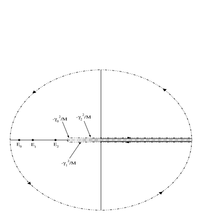
Figure 5.1: The singularity structure of an example of the full Green’s function for complex $E$ with three three-body bound states and three two-body bound states. Also shown is the contour $C$ used in the dispersion relation.

Now we know the analytic properties of ${\cal G}_{2B}(p)$, expression (5.30) can be used to obtain an analytic continuation of the projection operator, ${\cal P}(p)$. Using eqns. (5.27,5.30) we can write

$${\cal P}(p)=\frac{2\pi ip}{M}\Bigl{(}{\cal G}_{2B}(p)-{\cal G}_{2B}(-p)\Bigr{)}.$$ (5.32)

Due to the form of the equation we cannot readily continue the projection operator into the complex $p$-plane without assumptions on the analytic properties of ${\cal G}_{2B}(p)$ in the lower half of the complex plane.

Eqn. (5.32) is the generalisation (in unscaled coordinates) of eqn. (3.94) and provides us with the means to solve the 3BDWRG quite generally .

5.4 The Solution of the 3BDWRG for “Well-behaved” Pairwise Forces.

If the pairwise forces are “well-behaved” in the sense of section 3.6 then the distorted waves must vanish as $R^{2}$ as $R\rightarrow 0$. We can immediately write down a form for the full Green’s function and the distorted waves at the point at which the three-body force acts $\bar{R},\,\bar{\alpha}$,

$$\displaystyle{\qquad|\Psi_{\Lambda,k}(\bar{R},\bar{\alpha})|^{2}=\Lambda^{4}\bar{R}^{4}|\varphi(\bar{\alpha})|^{2}{\cal D}_{3}(k/\Lambda,\kappa_{i}/\Lambda),}$$ (5.33)

$$\displaystyle{\qquad|\Psi_{\Lambda,\gamma_{n}}(\bar{R},\bar{\alpha})|^{2}=\Lambda^{5}\bar{R}^{4}|\varphi(\bar{\alpha})|^{2}{\cal D}_{2}^{n}(\kappa_{i}/\Lambda),}$$ (5.34)

$$\displaystyle{\langle\bar{R},\bar{\alpha}|{\cal G}_{2B}(\Lambda)|\bar{R},\bar{\alpha}\rangle=M\Lambda^{4}\bar{R}^{4}|\varphi(\bar{\alpha})|^{2}{\cal D}_{G}(\kappa_{i}/\Lambda),}$$ (5.35)

where $\varphi(\bar{\alpha})$ is an unimportant functions that describes the hyperangular behaviour of the DWs close to the origin. Inserting these forms into eqn. (5.24), the correct rescaling for the three-body force is,

$$\hat{V}_{3B}(\hat{p},\hat{\kappa}_{i};\hat{k},\hat{k}^{\prime};\Lambda)=\frac{M\bar{R}^{5}\Lambda^{4}}{2\pi^{2}}V_{3B}(\Lambda\hat{p},\Lambda\hat{\kappa}_{i};\Lambda\hat{k},\Lambda,\hat{k}^{\prime},\Lambda).$$ (5.36)

Resulting in the 3BDWRG equation,

$$\displaystyle{\Lambda\frac{\partial\hat{V}_{3B}}{\partial\Lambda}=\hat{p}\frac{\partial\hat{V}_{3B}}{\partial\hat{p}}+\sum_{i}\hat{\kappa}_{i}\frac{\partial\hat{V}_{3B}}{\partial\hat{\kappa}_{i}}+\hat{k}\frac{\partial\hat{V}_{3B}}{\partial\hat{k}}+\hat{k}^{\prime}\frac{\partial\hat{V}_{3B}}{\partial\hat{k}^{\prime}}+4\hat{V}_{3B}}$$

$$\displaystyle{\,\,\,\,\,\,\,\,+\frac{1}{1-\hat{p}^{2}}\Biggl{[}\sum_{\gamma_{n}}\hat{V}_{3B}(\hat{p},\hat{\kappa}_{i};\hat{k},i\hat{\gamma}_{n};\Lambda)\hat{V}_{3B}(\hat{p},\hat{\kappa}_{i};i\hat{\gamma}_{n},\hat{k}^{\prime};\Lambda){\cal D}_{2}^{n}(\hat{\kappa}_{i})}$$

$$\displaystyle{\qquad\,\,\,\,+\frac{2}{\pi}\int_{0}^{1}d\hat{k}^{\prime\prime}\hat{V}_{3B}(\hat{p},\hat{\kappa}_{i};\hat{k},\hat{k}^{\prime\prime};\Lambda)\hat{V}_{3B}(\hat{p},\hat{\kappa}_{i};\hat{k}^{\prime\prime},\hat{k}^{\prime};\Lambda){\cal D}_{3}(\hat{k}^{\prime\prime},\hat{\kappa}_{i})\Biggr{]}.}$$ (5.37)

This equation is quite complicated as it has to describe the coupling of the three-body force to each of the distorted waves. The trivial fixed point solution, $\hat{V}_{3B}=0$, corresponds to a zero three-body force. The perturbations around it,

$$\hat{V}_{3B}=\sum_{l_{i},m,n,n^{\prime}=0}^{\infty}\hat{C}_{l_{i},m,n,n^{\prime}}\left(\frac{\Lambda}{\Lambda_{0}}\right)^{\nu}\hat{\kappa}_{i}^{l_{i}}\hat{p}^{2m}\hat{k}^{2n}\hat{k}^{\prime 2n^{\prime}},$$ (5.38)

have RG eigenvalues $\nu=2m+2n+2n^{\prime}+\sum l_{i}+4=4,(5),6\ldots$. All the eigenvalues are positive so the fixed point is stable. This fixed point is simply Weinberg counting, in which the first three-body force term occurs at $(Q/\Lambda_{0})^{4}$.

To find a non-trivial fixed point solution, we generalise the arguments of section 3.6. A non-trivial fixed point that is independent of the momentum variables may be found by solving the equation,

$$\hat{p}\frac{\partial\hat{V}_{3B}^{-1}}{\partial\hat{p}}+\hat{\kappa}_{i}\frac{\partial\hat{V}_{3B}^{-1}}{\partial\hat{\kappa}_{i}}-4\hat{V}_{3B}^{-1}-\frac{2\pi i}{1-\hat{p}^{2}}\Bigl{(}{\cal D}_{G}(\hat{\kappa}_{i})-{\cal D}_{G}(-\hat{\kappa}_{i})\Bigr{)}=0,$$ (5.39)

which comes from using the form for the projection operator (5.32). This is solved by the contour integration,

$$\frac{1}{\hat{V}_{3B}^{(0)}}=2\pi i\int_{C}d\hat{q}\frac{\hat{q}^{5}}{\hat{p}^{2}-\hat{q}^{2}}{\cal D}_{G}(\hat{\kappa}_{i}/\hat{q}).$$ (5.40)

where $C$ is a contour going from $-1$ to $1$ via the upper-half of the complex $\hat{q}$-plane outside all three-body bound state poles and two-body elastic thresholds on the imaginary axis. This solution is analytic in $\hat{p}$ but may have simple logarithmic dependence on some of the scales that can be removed using counterterms with logarithmic dependence on $\Lambda$. The momentum-independent perturbations around this fixed point solution take the form

$$\frac{1}{\hat{V}_{3B}}=\frac{1}{\hat{V}_{3B}^{(0)}}+\sum_{l_{i},m=0}^{\infty}\hat{C}_{l_{i},m,n,n^{\prime}}\left(\frac{\Lambda}{\Lambda_{0}}\right)^{\nu}\hat{\kappa}_{i}^{l_{i}}\hat{p}^{2m},$$ (5.41)

with RG eigenvalues $\nu=2m+l_{i}-4=-4,(-3),-2,\ldots$. This fixed point is unstable with 2 energy-dependent unstable perturbations and possibly 2 more $\kappa_{i}$-dependent unstable perturbations. Like the power-counting schemes in the two-body higher partial waves it seems implausible that this fixed point is ever likely to provide a useful expansion in physical systems because of the fine-tuning required in the unstable perturbations.

5.5 Three Body Force in the KSW EFT for Short Range Forces

In this section we will return to the EFT considered in the chapter 2 and its extension to systems of three particles. When we construct an EFT Lagrangian, we have to include all terms that do not violate the observed symmetries of the system. In a system in which all energies are far lower than the inverse range of the interactions this leads to a Lagrangian containing not only all the four-point vertex interactions (including derivative couplings) that correspond to the energy-dependent contact potentials but also to six-point and higher vertex interactions needed to model interaction channels that only become available in the presence of more than two particles. Of course the six point interactions are only required in a system with at least three particles, while the eight point terms require four particles and so on. The two-body couplings are entirely determined by two-body observables and should be taken as given when considering a three-body system. The three-body couplings are fixed by three-body observables.

In reactions between a bound pair and a third particle the pair-wise interactions result in a long range force due to the exchange of one particle. The range of this force is comparable to the scattering length of the two-body interaction.

If the two-body system is weakly interacting, the correct power-counting in the two-body system is the Weinberg system. The two-body scattering length $a_{2}\sim 1/\Lambda_{0}$, and hence provides a short-range exchange interaction. This system does not provide any particular difficulty in the three-body system since we can use naive dimensional analysis to determine at which order each diagram occurs. In this expansion the three-body force occurs at $(Q/\Lambda_{0})^{4}$ as in the previous example. (There is, of course, the alternative finely-tuned three-body force outlined in the previous example.)

In a KSW system the fine tuning of the LO perturbation around the non-trivial fixed point of the RG results in a large scattering length, $1/a_{2}\sim Q\ll 1/\Lambda_{0}$, and hence a long-range exchange interaction. This causes a significant complication as all the diagrams involving the leading four-point vertex need to be resummed[66, 22]. Since naive dimensional analysis is no longer applicable the power-counting for the three-body forces must be determined by renormalisation of the diagrams to which they contribute.

The 3BDWRG allows us to resum the effects of these diagrams and promote them to a fixed point. In the KSW EFT we need only resum the effects of the scattering length terms since it must be treated as a low-energy scale, it is not necessary to resum the effects of the effective range terms since these are perturbative $1/r_{2}\sim\Lambda_{0}$

The study of this problem has a long history. Skorniakov and Ter-Martirosian (STM) [56] were the first to derive equations for a system of a bound pair and particle with two-body contact interactions defined solely by a scattering length. There work was followed up by Danilov[57] who realised that in some systems the STM equations did not have unique solutions and required the input of a single piece of three-body data, namely the binding energy of the three-body state. The work of both of these predates that of Faddeev [58] in resolving the disconnected nature of the three-body equations. The STM equations rely upon the zero range nature of the two-body interaction to reduce the problem to a one-dimensional equation.

An alternative approach to the problem was given by Efimov [25]. Efimov’s equations show the singular nature of the system far more transparently than those of Skorniakov and Ter-Martirosian. We shall look at these equations below: in a nutshell Efimov’s approach allows us to express the system in terms of a hyperradial inverse square potential. The strength of the potential depends upon the statistics of the system. In the case of three Bosons and three nucleons in the ${}^{3}S_{1}$ channel the inverse square potential is attractive and hence singular, requiring a choice of self-adjoint extension.

Since the conception of EFTs this system and the related singular inverse square potential have received much attention [22, 24, 30, 31, 32, 33, 34, 23]. In particular, Bedaque et al [22, 24] have used extended versions of the STM equations to create a EFT that has proven highly effective in describing three-body data. In nuclear systems, the so-called pionless EFT proves effective in the s-wave $J=3/2$ system [66] and in higher angular momentum systems [59] without three-body forces. These systems are repulsive at short distances because of the centrifugal barrier or the Pauli exclusion principle and are therefore insensitive to short distance physics and three-body interactions. In Efimov’s approach these systems correspond to repulsive hyperangular inverse square potentials and so, from the DWRG analysis in section 3.5, the power-countings correspond to a weak system with LO three-body force scaling with $(Q/\Lambda_{0})^{2\nu}$ or a finely-tuned system with a LO three-body force scaling with $(Q/\Lambda_{0})^{-2\nu}$ where $\nu$ is the strength of the hyperangular potential. Given the apparent success achieved without three-body forces the first counting is appropriate. These systems are now well understood and we shall not concern ourselves with them.

The systems that correspond to singular hyperangular potentials are still being studied. Bedaque et al have incorporated three-body forces into the STM equations and used them to resolve the singular behaviour of these system [22, 24]. The effective three-body forces contain free parameters that must be fixed by fitting to three-body data. The power-counting proposed by Bedaque et al has three-body forces occurring at orders $(Q/\Lambda_{0})^{2n}$ where $n=0,1,2,\ldots$. The LO force is marginal. Each of the three-body force terms have cyclic behaviour in the cut-off, $\Lambda$. Phillips and Afnan [33] have also looked at the problem, their solution is to incorporate the 2+1 scattering length into the equations in a manner that ‘fixes’ the singularity and ensures that they give the correct 2+1 scattering length. The input of a single piece of three-body data is surely equivalent to the LO three-body force of Bedaque et al and both are equivalent to a particular choice of self-adjoint extension of the Hamiltonian. The difference in their stances is in attributing it to a three-body force and the need for higher order three-body forces.

In this section we shall introduce Efimov’s equations for three Bosons and explicitly demonstrate the connection between the inverse square potential and the KSW EFT three-body problem. We shall discuss the case of infinite two-body scattering length, where Efimov’s equations may be solved analytically, and show that in this case the power-counting for the three-body force is the same as proposed by Bedaque et al[24]. We shall then use the 3BDWRG to discuss the more general case of systems with finite two-body scattering length. We will show that the introduction of a finite scattering length does not change the power-counting for the three-body force and that the 3BDWRG solution is governed by a limit-cycle solution.

5.5.1 Efimov’s Equations

The two-body interaction may be written as a boundary condition on the wavefunction at zero separation. The full three-body wavefunction, $|\Psi\rangle$, is defined by the wave equation and the three boundary conditions,

$$\displaystyle{\qquad\qquad(H_{0}-E)|\Psi\rangle=0,}$$ (5.42)

$$\displaystyle{\left[\frac{\partial}{\partial x_{ij}}x_{ij}\langle{\bf x}_{ij},{\bf y}_{k}|\Psi\rangle\right]_{x_{ij}=0}=\left[a_{2}^{-1}x_{ij}\langle{\bf x}_{ij},{\bf y}_{k}|\Psi\rangle\right]_{x_{ij}=0}.}$$ (5.43)

From here we shall drop the particle number indices by writing the wavefunction in terms of the permutation operator, $P$,

$$|\Psi\rangle=(1+P)|\psi\rangle.$$ (5.44)

Substituting this form into eqn. (5.43) we obtain,

$$\left[\frac{\partial}{\partial x}x\langle{\bf x},{\bf y}|\psi\rangle+\langle{\bf x},{\bf y}|P|\psi\rangle\right]_{x=0}=\left[a_{2}^{-1}x\langle{\bf x},{\bf y}|\psi\rangle\right]_{x=0}.$$ (5.45)

We consider the case of zero angular momentum and write the wavefunction as $\psi(x,y)=xy\langle{\bf x},{\bf y}|\psi\rangle$, so that eqns.(5.42,5.45) become,

$$\displaystyle{\qquad\qquad\left(\frac{\partial^{2}}{\partial x^{2}}+\frac{3}{4}\frac{\partial^{2}}{\partial y^{2}}+ME\right)\psi(x,y)=0},$$ (5.46)

$$\displaystyle{\left[\frac{\partial\psi(x,y)}{\partial x}\right]_{x=0}+\frac{4}{y}\psi\left(y,\frac{1}{2}y\right)=a_{2}^{-1}\psi(0,y).}$$ (5.47)

In addition we have the boundary condition which follows from the definition of $\psi$: $\psi(x,0)=0$. Eqns.(5.46,5.47) are the wave equation with non-trivial boundary condition and are, in general, extremely difficult to solve. To examine them more closely we rewrite them in terms of the hyperpolar coordinates, $x=R\cos\alpha,y=\sqrt{3}/2R\sin\alpha$,

$$\displaystyle{\,\,\,\,\left(\frac{\partial^{2}}{\partial R^{2}}+\frac{1}{R}\frac{\partial}{\partial R}+\frac{1}{R^{2}}\frac{\partial^{2}}{\partial\alpha^{2}}+ME\right)\psi(R,\alpha)}=0,$$ (5.48)

$$\displaystyle{\left[\frac{\partial\psi(R,\alpha)}{\partial\alpha}\right]_{\alpha=\pi/2}+\frac{8}{\sqrt{3}}\psi\left(R,\frac{\pi}{6}\right)=Ra_{2}^{-1}\psi\left(R,\frac{\pi}{2}\right)}.$$ (5.49)

These provide us with the information we require to study the DWRG in this problem.

5.5.2 The Infinite Scattering Length Limit.

Efimov’s equations, (5.48,5.49) may be solved analytically in the limit of infinite scattering length. We shall turn our attention to this case as it is considerably simpler than the more general case of finite scattering length. In the limit $a_{2}\rightarrow\infty$ the boundary condition becomes separable. Writing,

$$\psi(R,\alpha)=F_{s}(R)\sin s\alpha,$$ (5.50)

we obtain,

$$\displaystyle{\left(\frac{\partial^{2}}{\partial R^{2}}+\frac{1}{R}\frac{\partial}{\partial R}-\frac{s^{2}}{R^{2}}+p^{2}\right)F_{s}(R)}=0,$$ (5.51)

$$\displaystyle{\qquad-s\cos\frac{s\pi}{2}+\frac{8}{\sqrt{3}}\sin{\frac{s\pi}{6}}=0},$$ (5.52)

where $p=\sqrt{ME}$. These equations are now a simple matter to solve. The transcendental equation (5.52) must be solved numerically. It has two imaginary solutions $s_{0}=\pm i1.006237\ldots$ and an infinite number of real solutions, the smallest of which is $s_{1}=4$. The imaginary roots of Eqn.(5.52) result in an attractive inverse square potential for the hyperradial equation (5.51) while the real roots give repulsive potentials.

The hyperradial part of the wavefunction is given by,

$$F_{s}(R;p)=\begin{cases}\sqrt{\frac{\pi p}{2}}J_{s}(pR)\qquad\text{if}\qquad s\in{\mathbb{R}}\\ \sqrt{\frac{\pi p}{2}}(2i|\sin(\eta(p)+i\pi\bar{s}_{i}/2)|)^{-1}\Bigl{(}e^{i\eta(p)}J_{i\bar{s}}(pR)-e^{-i\eta(p)}J_{-i\bar{s}}(pR)\Bigr{)}\qquad\text{if}\qquad s\not\in{\mathbb{R}},\end{cases}$$ (5.53)

where $\bar{s}=\text{Im}{s}$. In the imaginary hyperangular momentum channel, since this is an attractive channel, we have, as was necessary, defined a self-adjoint extension of the Hamiltonian by choosing a phase, $\eta(p)$. The bound states of the system only occur in this channel and are given, in parallel to the bound states of the attractive inverse square potential, by

$$F_{s}^{(n)}(R)=\sqrt{\frac{2\sinh(\pi\bar{s})}{\pi\bar{s}}}p_{n}K_{i\bar{s}}(p_{n}R).$$ (5.54)

These states, like the attractive inverse square potential, form an infinite tower of bound states. The lack of a ground state in three body system acting under such forces was first noted by Thomas[26] and is known as the Thomas effect; of course such a state of affairs is a result of an inexact treatment of short-range physics and will be resolved by the EFT precisely as it was in the chapter 4. The accumulation of bound states at zero energy is due to the tail of the inverse square potential, and hence a result of this special case of infinite scattering length. These states are known as Efimov states [25] and are not a result of any mistreatment of physics but are genuine phenomena .

Since the Hamiltonian conserves hyperangular momentum we can expand any three body scattering amplitude in terms of the hyperangular eigenfunctions and corresponding hyper-phaseshifts. This makes the DWRG analysis particularly simple since the equations become one-dimensional. The effect of the three-body force may be analysed in each hyperangular channel, in other words dependence upon the unconstrained external momentum terms $k$ and $k^{\prime}$, favoured earlier in the chapter, can be dropped in favour of dependence upon the hyperangular momentum $s$. The differential equation for the three body force in each channel is then,

$$\displaystyle{\qquad\qquad\frac{\partial V_{3B}^{(s)}(p,\Lambda)}{\partial\Lambda}=\frac{M\bar{R}}{2\pi^{2}}\frac{|\Psi_{\Lambda,s}(\bar{R},\bar{\alpha})|^{2}}{\Lambda^{2}-p^{2}}V_{3B}^{(s)}(p,\Lambda)^{2}\qquad\text{ if }s\in{\mathbb{R}},}$$ (5.55)

$$\displaystyle{\frac{\partial V_{3B}^{(s)}(p,\Lambda)}{\partial\Lambda}=\frac{M\bar{R}}{2\pi^{2}}\left(\frac{|\Psi_{\Lambda,s}(\bar{R},\bar{\alpha})|^{2}}{\Lambda^{2}-p^{2}}-\frac{\pi}{2}\sum_{n}\delta(\Lambda-|p_{n}|)\frac{|\Psi_{s}^{(n)}(\bar{R},\bar{\alpha})|^{2}}{p^{2}+p_{n}^{2}}\right)V_{3B}^{(s)}(p,\Lambda)^{2}}$$

$$\displaystyle{\qquad\qquad\qquad\qquad\qquad\qquad\qquad\qquad\qquad\qquad\qquad\qquad\qquad\text{ if }s\not\in{\mathbb{R}}.}$$ (5.56)

In the repulsive channels (real $s$) the resulting DWRG equation is precisely that considered in section 3.5 and the analysis there can be followed to obtain the power-counting for the three-body force in those channels. The effects of the force can be expressed as a distorted wave Born or effective range expansion for the correction to the hyper-phaseshift. Following the discussion in section 3.5 the fine-tuning required for a non-trivial fixed point power-counting for these forces would be rather contrived. For example, the least repulsive channel has the eigenvalue $s_{1}=4$ and would require three unnaturally small parameters to ensure the RG flow remained in the region of the non-trivial fixed point. Hence, the appropriate power-counting for the three-body force in these channels is based upon the trivial fixed point and provides only very small (at least of order $(Q/\Lambda_{0})^{4}$) contributions to the scattering observables.

In the attractive channels we must turn to the analysis considered of chapter 4. The DWRG analysis is precisely as found there and is very different from that in the repulsive channels and results in a three-body force that contributes at a surprisingly low order, $(Q/\Lambda_{0})^{0}$, to the scattering observables. In this role it is more important than effective range corrections which occur at an order, $(Q/\Lambda_{0})^{1}$. This power-counting for the three-body force agrees with Bedaque et al [24].

The implications, for both EFT and potential modelling of the three-body problem, of such a prominent three-body force will be examined later. Before then we shall show how the DWRG analysis for the three body force needs to be modified after the introduction of a finite two-body scattering length.

The method outlined in this section is useful because everything may be dealt with analytically. However, in order to fully grasp the general problem with finite scattering length, our general analysis must be based upon the the 3BDWRG. This not only allows us to deal with the problem of the different channels but also allows us to presents results for observables in more practical format.

5.5.3 Finite Scattering Length

The Distorted Waves and the DWRG Equation

In reaching eqns.(5.51,5.52) we took the two-body scattering length to infinity. This limit is of course also reached if we take the hyperradius to zero, meaning that at small hyperradii the general distorted waves have the same functional form (in $R$) as their infinite scattering length counterparts. In particular we must have for any DW,

$$\Psi(R,\alpha)={\cal D}\varphi(\alpha)\sin(\bar{s}_{0}\ln p_{*}R),$$ (5.57)

where we must chose the scale $p_{*}$ in order to define a self-adjoint extension. The magnitude of the DWs close to the origin will in general depend upon the two-body scattering length. As in the attractive inverse square case, the relationship between self-adjoint extensions and $p_{*}$ is not one-to-one. All observables are invariant under the transformation,

$$p_{*}\rightarrow p_{*}e^{\pi n/\bar{s}_{0}}.$$ (5.58)

where $\bar{s}_{0}=1.00623\ldots$ is the magnitude of the imaginary solution of eqn. (5.52).

The Green’s function, since it solves the Schrödinger equation, also observes the behaviour (5.57). We write the Green’s function matrix elements evaluated at small hyperradius as

$$\langle\bar{R},\bar{\alpha}|{\cal G}_{2B}(p)|\bar{R},\bar{\alpha}\rangle=M{\cal D}_{G}\left(\gamma/p,\ln p/p_{*}\right)|\varphi(\bar{\alpha})|^{2}\sin^{2}\left(\bar{s}_{0}\ln{p_{*}\bar{R}}\right),$$ (5.59)

where $\gamma=1/a_{2}$ is the binding momentum of the two-body bound state. Because of the relationship (5.58), ${\cal D}_{G}(x,y)$ is periodic in $y$ with period $2\pi/\bar{s}_{0}$. All the analytic properties of ${\cal G}_{2B}(p)$ as a function of $p$, described earlier, are conferred on the function ${\cal D}_{G}$. Namely, there is the elastic two-body scattering cut at $p=i\gamma$ that runs down the imaginary $p$ axis then along the real axis and there are poles at each of the bound states.

The singular behaviour at small hyperradii that leads to the trig-log behaviour in the DWs also means that there is no ground state. At very high momentum the two-body scattering length becomes insignificant and the DWs take the form they would in the limit $\gamma\rightarrow 0$. This means that the deeply bound state take on the geometrically spaced form of the attractive inverse square potential’s states. At low energies the value of $\gamma$ is important and disrupts the exponential ladder of bound states; the Efimov effect no longer occurs.

The lack of a ground state means that, as in chapter 4, we must truncate the full Green’s function in both the continuum and bound states. Notice there is no need to continue this truncation into the elastic threshold since this is controlled by the low-energy scale $\gamma$. The result of truncating the bound states is slightly more complicated than in the attractive inverse square example because the position of each bound state is not only controlled by the high-energy scale $p_{*}$ but also by the low-energy scale $\gamma$. The effect this has on the renormalisation group flow is important and requires careful consideration.

For the individual distorted waves we write down the forms for small $\bar{R}$ as

$$\displaystyle{|\Psi_{p,k}(\bar{R},\bar{\alpha})|^{2}={\cal D}_{3}\left(\frac{k}{p},\frac{\gamma}{p},\ln\frac{p}{p_{*}}\right)|\varphi(\bar{\alpha})|^{2}\sin^{2}\left(\bar{s}_{0}\ln p_{*}\bar{R}\right),}$$ (5.60)

$$\displaystyle{|\Psi_{p,\gamma}(\bar{R},\bar{\alpha})|^{2}=p{\cal D}_{2}\left(\frac{\gamma}{p},\ln\frac{p}{p_{*}}\right)|\varphi(\bar{\alpha})|^{2}\sin^{2}\left(\bar{s}_{0}\ln p_{*}\bar{R}\right),}$$ (5.61)

$$\displaystyle{|\Psi_{n}(\bar{R},\bar{\alpha})|^{2}=p_{n}(\gamma,p_{*})^{2}{\cal D}_{B}\left(\gamma,p_{n}(\gamma,p_{*})\right)|\varphi(\bar{\alpha})|^{2}\sin^{2}\left(\bar{s}_{0}\ln{p_{*}\bar{R}}\right),}$$ (5.62)

where we have explicitly shown the dependence of the binding momenta, $p_{n}$, on $\gamma$ and $p_{*}$. From eqn. (5.28) it follows that ${\cal D}_{B}(\gamma,p_{n})$ can simply be found by taking the residue of the Green’s function at the appropriate bound state pole to give,

$${\cal D}_{B}(\gamma,p_{n})=\frac{8\pi i}{p_{n}}{\cal R}\{{\cal D}_{G}(\gamma/p,\ln p/p_{*}),p\rightarrow ip_{n}\}.$$ (5.63)

The projection operator matrix element for small $\bar{R}$ and $p^{2}>0$ follow from its definition (5.18),

$$\langle\bar{R},\bar{\alpha}|{\cal P}(p)|\bar{R},\bar{\alpha}\rangle=p{\cal C}\left(\frac{\gamma}{p},\ln\frac{p}{p_{*}}\right)|\varphi(\bar{\alpha})|^{2}\sin^{2}\left(\bar{s}_{0}\ln{p_{*}\bar{R}}\right),$$ (5.64)

where

$${\cal C}\left(\frac{\gamma}{p},\ln\frac{p}{p_{*}}\right)={\cal D}_{2}\left(\frac{\gamma}{p},\ln\frac{p}{p_{*}}\right)+\frac{2}{\pi}\int_{0}^{p}dk{\cal D}_{3}\left(\frac{k}{p},\frac{\gamma}{p},\ln\frac{p}{p_{*}}\right).$$ (5.65)

The function ${\cal C}$ may also be written using eqn. (5.32) as,

$${\cal C}\left(\frac{\gamma}{p},\ln\frac{p}{p_{*}}\right)=2\pi i\left[{\cal D}_{G}\left(\frac{\gamma}{p},\ln\frac{p}{p_{*}}\right)-{\cal D}_{G}\left(\frac{-\gamma}{p},\ln\frac{p}{p_{*}}+i\pi\right)\right].$$ (5.66)

We are now in a position to rescale the differential equation for $V_{3B}$ to obtain the DWRG equation. The scales $p,\gamma,k$ and $k^{\prime}$ rescale in the usual way. The three-body force is rescaled by the relation,

$$\hat{V}_{3B}(\hat{p},\hat{\gamma};\hat{k},\hat{k}^{\prime};\Lambda)=\frac{M\bar{R}}{2\pi^{2}}|\varphi(\bar{\alpha})|^{2}\sin^{2}\left(\bar{s}_{0}\ln{p_{*}\bar{R}}\right)V_{3B}(\Lambda\hat{p},\Lambda\hat{\gamma};\Lambda\hat{k},\Lambda\hat{k}^{\prime};\Lambda).$$ (5.67)

Using eqn.(5.24) with the addition of the truncated bound states the resulting DWRG for the three-body force is,

$$\displaystyle{\Lambda\frac{\partial\hat{V}_{3B}}{\partial\Lambda}=\hat{p}\frac{\partial\hat{V}_{3B}}{\partial\hat{p}}+\hat{\gamma}\frac{\partial\hat{V}_{3B}}{\partial\hat{\gamma}}+\hat{k}\frac{\partial\hat{V}_{3B}}{\partial\hat{k}}+\hat{k}^{\prime}\frac{\partial\hat{V}_{3B}}{\partial\hat{k}^{\prime}}}$$

$$\displaystyle{\,\,\,\,+\frac{1}{1-\hat{p}^{2}}\Biggl{[}\hat{V}_{3B}(\hat{p},\hat{\gamma};\hat{k},i\hat{\gamma};\Lambda)\hat{V}_{3B}(\hat{p},\hat{\gamma};i\hat{\gamma},\hat{k}^{\prime};\Lambda){\cal D}_{2}(\hat{\gamma},\ln\Lambda/p_{*})}$$

$$\displaystyle{\qquad+\frac{2}{\pi}\int_{0}^{1}d\hat{k}^{\prime\prime}\hat{V}_{3B}(\hat{p},\hat{\gamma};\hat{k},\hat{k}^{\prime\prime};\Lambda)\hat{V}_{3B}(\hat{p},\hat{\gamma};\hat{k}^{\prime\prime},\hat{k}^{\prime};\Lambda){\cal D}_{3}(\hat{k}^{\prime\prime},\hat{\gamma},\ln\Lambda/p_{*})\Biggr{]}}$$

$$\displaystyle{-\frac{\pi}{2}\sum_{n}\hat{V}_{3B}(\hat{p},\hat{\gamma};\hat{k},i/3;\Lambda)\hat{V}_{3B}(\hat{p},\hat{\gamma};i/3,\hat{k}^{\prime};\Lambda)\frac{\delta(\Lambda-p_{n}(\Lambda\hat{\gamma},p_{*}))\Lambda}{1+\hat{p}^{2}}{\cal D}_{B}(\hat{\gamma}/\hat{p}_{n},\ln p_{n}/p_{*}).}$$

(5.68)

where we have suppressed the obvious functional dependence of $\hat{V}_{3B}$ in the terms on the first line to save space.

The perturbations around the trivial fixed point solution, $\hat{V}_{3B}=0$, are given by,

$$\hat{V}_{3B}=\sum_{k,l,m,n}\hat{C}_{l,m,n,n^{\prime}}\hat{p}^{2m}\hat{k}^{2n}\hat{k}^{\prime 2n^{\prime}}\hat{\gamma}^{l}\left(\frac{\Lambda}{\Lambda_{0}}\right)^{l+2m+2n+2n^{\prime}}.$$ (5.69)

The leading order perturbation is marginal, this is consistent with the trivial fixed point solution in the attractive inverse square (zero $\hat{\gamma}$) solution. Like the attractive inverse square DWRG this solution means very little by itself and in order to determine the nature of the marginal perturbation and the general flow of the DWRG we must examine a more general solution. Like the attractive inverse square DWRG the marginal perturbation occurs because the basic loop integral solution is an example of a limit-cycle solution.

The Limit-Cycle DWRG solution.

We look now for a solution to the 3BDWRG equation that depends on $\Lambda$ logarithmically and that is independent of the momentum terms. This satisfies the 3BDWRG equation,

$$\Lambda\frac{\partial}{\partial\Lambda}\frac{1}{\hat{V}_{3B}}=\hat{p}\frac{\partial}{\partial\hat{p}}\frac{1}{\hat{V}_{3B}}+\hat{\gamma}\frac{\partial}{\partial\hat{\gamma}}\frac{1}{\hat{V}_{3B}}-\frac{{\cal C}(\hat{\gamma},\ln\Lambda/p_{*})}{1-\hat{p}^{2}}+\frac{\pi}{2}\sum_{n}\frac{\delta(\Lambda-p_{n}(\Lambda\hat{\gamma},p_{*}))\Lambda}{1+\hat{p}^{2}}{\cal D}_{B}(\hat{\gamma},\ln p_{n}/p_{*}).$$ (5.70)

The solution to this equation with logarithmic dependence upon $\Lambda$ may be constructed in much the same way as the solution to the attractive inverse square potential DWRG. We write the solution as the integral,

$$\frac{1}{\hat{V}_{3B}^{(0)}(\hat{p},\hat{\gamma},\Lambda)}=2\pi i\int_{C}d\hat{q}\frac{\hat{q}}{\hat{p}^{2}-\hat{q}^{2}}{\cal D}_{G}\left(\frac{\hat{\gamma}}{\hat{q}},\ln\frac{\Lambda\hat{q}}{p_{*}}\right),$$ (5.71)

where the contour $C$ is illustrated in Fig.5.2, it runs from $-1$ to $1$ through the upper half of the complex plane and crosses the imaginary axis at $\hat{q}=i$. Substitution and use of eqn. (5.66) shows that it satisfies the continuous part of the 3BDWRG equation. The integral is clearly analytic about $\hat{p}\rightarrow 0$ since the propagator poles to do not approach any part of the contour $C$ in this limit. The integral is also analytic as $\hat{\gamma}\rightarrow 0$ since it matches continuously onto the attractive inverse square solution in that limit. The discontinuities caused by the truncation of bound states result from allowing the bound state poles to cross the contour. That the residues of these poles produce the correct discontinuities is readily confirmed using eqn. (5.63).

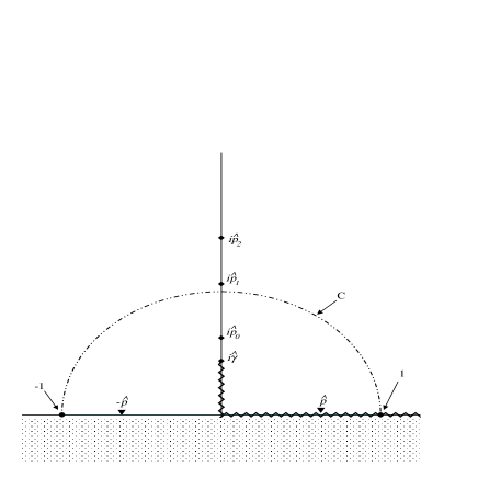
Figure 5.2: The singularity structure of the integrand in the limit cycle solution. The bound state poles occur at $\hat{q}=i\hat{p}_{n}$, the two-body elastic scattering threshold branch point occurs at $\hat{q}=i\hat{\gamma}$. The propagator poles occur at $\hat{q}=\pm\hat{p}$. The contour $C$ runs in a semi-circle from $-1$ to $1$ through the upper half of the complex plane and crosses the imaginary axis at $\hat{q}=i$.

The migration of the bound state poles up the imaginary axis is more complicated in this example than in the attractive inverse square case. The position of each bound state in the unscaled theory is determined by the scales $\gamma$ and $p_{*}$. In the rescaled theory they are determined by $\hat{\gamma}$ and the ratio $p_{*}/\Lambda$. This has the interesting consequence that as $\Lambda$ varies only that element of the rescaled poles position controlled by the high energy scale $p_{*}$ changes. The element controlled by $\gamma$, as low energy physics, remains fixed.

We know that the transformation $p_{*}\rightarrow p_{*}e^{\pi/\bar{s}_{0}}$ leaves the bound state spectrum unchanged. This transformation is equivalent, in the rescaled spectrum, to

$$\Lambda\rightarrow\Lambda e^{-\pi/\bar{s}_{0}},$$ (5.72)

which must therefore leave the rescaled spectrum unchanged.

As $\Lambda$ decreases the poles move up the imaginary $\hat{q}$ axis. To ensure the rescaled bound states poles are invariant under transformation (5.72), new poles must ‘condense’ out of the elastic threshold cut when necessary.

The solution (5.71) describes a logarithmically evolving limit cycle solution. This can be seen by observing that since ${\cal D}_{G}(x,y)={\cal D}_{G}(x,y+2\pi/\bar{s}_{0})$,

$$\hat{V}_{3B}^{(0)}(\hat{p},\hat{\gamma},\Lambda)=\hat{V}_{3B}^{(0)}(\hat{p},\hat{\gamma},\Lambda e^{2\pi n/\bar{s}_{0}}).$$ (5.73)

This cyclic behaviour means that there must be an infinite number of geometrically spaced discontinuities as $\Lambda$ goes to either zero or infinity. At first it seems strange that we should be able to produce an infinite number of discontinuities as $\Lambda\rightarrow 0$ because for any particular $\Lambda$ there are only a finite number of bound state poles inside the contour $C$ in the complex $\hat{q}$-plane. However, bearing in mind the discussion above we can see that as $\Lambda\rightarrow 0$ more rescaled bound states appear and, because of eqn. (5.72), these will cross the contours in a strictly geometrically spaced pattern.

The limit cycle behaviour is only exact in the rescaled theory. The unscaled potential will approximate the limit cycle when $\Lambda\gg\gamma$ but as $\Lambda$ becomes less than $\gamma$ it will deviate significantly from it.

The momentum independent perturbations around the limit-cycle solution take the form observed in chapter 4,

$$\frac{1}{\hat{V}_{3B}}(\hat{p},\hat{\gamma},\Lambda)=\frac{1}{\hat{V}_{3B}^{(0)}}(\hat{p},\hat{\gamma},\Lambda)+\sum_{n,m=0}^{\infty}\hat{C}_{2n,m}\left(\frac{\Lambda}{\Lambda_{0}}\right)^{2n+m}\hat{p}^{2n}\gamma^{m}.$$ (5.74)

The marginal perturbation $\hat{C}_{0,0}$ must, as in the inverse square case, embody the same degree of freedom as the self-adjoint extension defining scale, $p_{*}$. The DWRG flow is very much as described in section 3.3 and as illustrated in Figs. 4.2,4.3.

This momentum independent solution may be substituted into the three-body distorted wave Lippmann-Schwinger equation (5.8) to obtain results for the $\tilde{T}_{3B}$-matrix. The analysis follows much the same form of that in section 2.6. In this case the truncated Green’s function also includes the integral around the branch cut along the imaginary axis, which corresponds to elastic bound pair and particle scattering. The result is

$$\displaystyle{\left[{\cal D}_{3}\left(\frac{k}{p},\frac{\gamma}{p},\ln\frac{p}{p}_{*}\right){\cal D}_{3}\left(\frac{k^{\prime}}{p},\frac{\gamma}{p},\ln\frac{p}{p}_{*}\right)\right]^{1/2}\langle\Psi_{p,k}|\tilde{\cal T}_{3B}|\Psi_{p,k^{\prime}}\rangle^{-1}-M{\cal D}_{G}\left(\frac{\gamma}{p},\ln\frac{p}{p}_{*}\right)}$$

$$\displaystyle{\qquad\qquad\qquad\qquad\qquad\qquad\qquad\qquad\qquad=\frac{M}{2\pi^{2}}\sum_{m,n=0}{\hat{C}}_{2n,m}\frac{p^{2n}\gamma^{m}}{\Lambda_{0}^{2n+m}}}$$ (5.75)

for a general $3\rightarrow 3$ scattering. For elastic scattering of a bound pair and a single particle we may write the $\tilde{\cal T}_{3B}$ matrix element in terms of a correction to the phaseshift in accordance with eqn. (3.14). The DWRG limit-cycle potential then yields the DWERE,

$${\cal D}_{2}\left(\frac{\gamma}{p},\ln\frac{p}{p}_{*}\right)(\cot\tilde{\delta}_{3B}-i)+4\pi{\cal D}_{G}\left(\frac{\gamma}{p},\ln\frac{p}{p}_{*}\right)=-\frac{2}{\pi}\sum_{m,n=0}{\hat{C}}_{2n,m}\frac{p^{2n}\gamma^{m}}{\Lambda_{0}^{2n+m}}.$$ (5.76)

If we have $p^{2}<0$ then by eqns. (5.65,5.66) we have,

$$4\pi\,\text{Im}{\cal D}_{G}\left(\frac{\gamma}{p},\ln\frac{p}{p}_{*}\right)={\cal D}_{2}\left(\frac{\gamma}{p},\ln\frac{p}{p}_{*}\right),$$ (5.77)

so that the imaginary parts on the LHS of eqn. (5.76) cancel and the correction to the phaseshift, $\tilde{\delta}_{3B}$ is real. If $p^{2}>0$ then eqn.(5.77) no longer holds because of the $3\rightarrow 3$ states.

The results above are for the momentum independent solutions of the DWRG only. More general solutions to the DWRG equations can be obtained by perturbing about the limit cycle solution with momentum dependent perturbations. These perturbations allow the three-body potential to differentiate between different types of DW. It is clear that they will be important in amplitudes like (5.75). However, in amplitudes such as (5.76) they will not provide any extra degrees of freedom in the power-counting since the external momenta $k$ and $k^{\prime}$ are set to $i\gamma$ in this amplitude. For completeness the momentum perturbations are found in Appendix D.

In any particular system that the EFT is describing the two-body bound state binding momentum, $\gamma$, is not adjustable. It is therefore impossible to determine the three-body force terms that correspond to these perturbations around the limit-cycle solution. For practical purposes these terms can be absorbed into the energy dependent perturbations to obtain for elastic scattering,

$${\cal D}_{2}\left(\frac{\gamma}{p},\ln\frac{p}{p}_{*}\right)(\cot\tilde{\delta}_{3B}-i)+4\pi{\cal D}_{G}\left(\frac{\gamma}{p},\ln\frac{p}{p}_{*}\right)=-\frac{2}{\pi}\sum_{m,n=0}{\hat{C}}_{2n}\left(\frac{p}{\Lambda_{0}}\right)^{2n}.$$ (5.78)

The power-counting in the energy dependent terms for the three-body force about the limit-cycle solution is precisely that found by Bedaque et al. The leading three-body force term is marginal and occurs at order $(Q/\Lambda_{0})^{0}$. This leading order force fixes the phase of the three-body DWs close to the origin, or equivalently forms a self-adjoint extension. The use of the DWRG method in deriving the power-counting for the three-body force in the EFT is a new result. It provides support for the work of Bedaque et al[22], which relies on introducing a dimer field into the EFT Lagrangian and then practical use of the three-body force to renormalise the theory order by order. Despite the power of their approach Bedaque et al cannot provide a simple algebraic statement of the power-counting nor a simple formula like (5.78).

When looked at from a different angle, our analysis means that the introduction of any three-body data to fix a self-adjoint extension such as was done by Phillips and Afnan [33] is equivalent to a LO three-body force. It is not necessary to explicitly calculate the three-body force. However, if we were to do so after fixing a self-adjoint extension we would find that the degree of freedom associated with that three-body force would be equivalent to that associated with the self-adjoint extension choice.

The RG methods used here are very different from those used by Hammer and Mehen [23], which start with the STM equation and supplement the approach of Bedaque et al [22, 24]. The STM equation can only describe three-body bound states and 2+1 scattering and so does not include all of the three-body physics. Furthermore, since the equations of Hammer and Mehen start from a truncated STM equation, part of the role of their three-body force is to restore the truncated part of the STM equation, a complication the DWRG method was designed to avoid. For similar reasons the form of our three-body force can not be directly compared to that given by Bedaque et al.

A limit cycle form of the three-body force in this EFT has been suggested by many previous papers[30, 32] that have essentially tackled the infinite scattering length case of the attractive inverse square problem. Bedaque et al also found a limit cycle solution but because of their approach could only find the force order by order [24].

Our result is also applicable to the three nucleon force in the pionless KSW EFT [24, 22, 65]. Braaten and Hammer have discussed the tuning of the quark masses in QCD required for an infra-red limit cycle in the three nucleon problem [65]. They assume that to obtain the scale invariant relationships that define a limit-cycle, such as (5.72), the system must be tuned to the infinite scattering length limit to avoid the introduction of scales that break the symmetry. The analysis here, which uses a Wilsonian RG approach, readily produces limit cycles in the rescaled potential since the low-energy quantities do not affect the symmetry. The discussion of Braaten and Hammer [65] applies to our unscaled potential, which only exhibits infra-red limit cycle behaviour in the infinite scattering length limit.

The complete 3BDWRG analysis in this system provides a concrete grounding for what has been intuitively understood. Beyond that, because of the common method of solving the DWRG equations in in this chapter and the previous two, the connection between all these results can be seen.

5.6 Summary

In this chapter we have examined the DWRG for three body forces. The approach used can be generalised quite simply to $N$-body forces. The 3BDWRG equation is complicated by this multi-channelled problem because the 3BDWRG has to describe the coupling of the three-body force to each of the different distorted waves.

The application of the 3BDWRG to the case of “well-behaved” potentials was included as an example. The two fixed points found correspond to Weinberg counting and to the three body equivalent of the KSW scheme. The instability of the non-trivial fixed point leads us to conclude that in almost all systems of this kind Weinberg counting and naive dimensional analysis is appropriate.

The 3BDWRG was also used to study three body forces in the KSW EFT. The solutions to the equation take the form of limit cycles and have much in common with the solutions found in chapter 4. The power counting found is marginal at leading order and matches that found by Bedaque et al [24].

Although our analysis has only considered the system of three Bosons, it is also appropriate for three nucleons in the ${}^{3}S_{1}$ channel as we shall see in the next chapter.

Chapter 6 The KSW Effective Field Theory of Three Bodies

A pionless KSW EFT for three nucleons has been successfully described by Bedaque et al [24, 66, 59]. Their work also covers the related system of three Bosons. We have seen in the previous chapter how the 3BDWRG analysis of the three-body force in this problem supports their conclusions. We shall now look to complement this work by deriving equations for the three body DWs.

All the predictive literature on the three body KSW EFT is concerned with scattering observables[24, 33]. However, some applications of the EFT require knowledge of the wavefunctions. For example, if we want to model scattering of an electron from the triton we need to know its charge density, which can be ascertained from the wavefunction.

The explicit solution of the equations for the DWs will also serve to illustrate the ‘phase-fixing’ role of the LO three-body force. We have seen in the 3BDWRG the equivalence of the choice of self-adjoint extension and the LO marginal term in the short range force. Because of this equivalence, the introduction of the three-body force at LO is a trivial matter of choosing a boundary condition for the poorly defined DWs.

As an introduction we shall consider the example of three Bosons. We shall then move on to the physically more interesting example of three nucleons.

6.1 The EFT for Three Bosons

The distorted waves for elastic scattering of a bound pair and a particle are not particularly easy to find using Efimov’s boundary conditions, although Fedorov and Jensen have attempted to develop a method of doing so [60]. We will derive equations for the DWs using a useful property of systems with zero range interactions. Namely, that the value of the DW may be simply determined from the value of the DW when the relative coordinate of a pair of particles is zero. Because the potential is zero at any point other than where two particles are ‘touching’, the value of the DW anywhere else may be found by integrating the wave equation. Skorniakov and Ter-Martirosian (STM)[56] were the first to take advantage of this property in their derivation of equations for the 2+1 scattering amplitude for zero range forces.

Our equations for the DWs will also use this property. We will derive equations that may be used to find all DWs below the three-body threshold. At one point in the derivation we will be able to link our method to the STM equations. Unlike Skorniakov and Ter-Martirosian, we will start our derivation with the Faddeev equation (5.11), which we rewrite here for convenience,

$$\displaystyle{\qquad\,\,\,\,\,\,|\Psi^{+}\rangle=(1+P)|\psi^{+}_{{\bf k}_{0}}\rangle},$$ (6.1)

$$\displaystyle{|\psi^{+}_{{\bf k}_{0}}\rangle=|\chi_{{\bf k}_{0}}\rangle+G_{0}^{+}(p)t^{+}(p)P|\psi^{+}_{{\bf k}_{0}}\rangle,}$$ (6.2)

where we have now labelled the wavefunctions by ${\bf k}_{0}$, the vector of the third particle in the centre of mass frame which has magnitude, $|{\bf k}_{0}|=\sqrt{4(p^{2}+\gamma^{2})/3}$, and $p^{2}=ME<0$ is the centre of mass energy, relative to the three-body threshold. Initially we will derive equations for the LO EFT, hence the two-body T-matrix is given simply by the scattering length term in the effective range expansion,

$$\displaystyle{\langle{\bf k,l}|t(p)|{\bf k^{\prime},l^{\prime}}\rangle=(2\pi)^{3}\delta^{3}({\bf k-k^{\prime}})\tau(p,k),}$$ (6.5)

$$\displaystyle{\qquad\tau(p,k)=-\frac{4\pi}{M}\left(-\gamma+i\sqrt{p^{2}-\frac{3}{4}k^{2}}\right)^{-1}.}$$ (6.6)

To make the importance of the zero separation value of the DWs apparent we will work in a mixed co-ordinate system $({\bf k},{\bf x})$, i.e. in terms of the distance between two particles and the momentum of the third particle in the centre of mass frame. Two matrix elements that will be needed are:

$$\displaystyle{\langle{\bf k,x}|G_{0}^{+}(p)t^{+}(p)|{\bf k^{\prime},x^{\prime}}\rangle=\tau(p,k^{\prime})L_{1}(p,{\bf k,k^{\prime},x})\delta^{3}({\bf x^{\prime}}),}$$ (6.7)

$$\displaystyle{\qquad\qquad\qquad L_{1}(p,{\bf k,k^{\prime},x})=-(2\pi)^{3}\delta^{3}({\bf k-k^{\prime}})\frac{M}{4\pi x}e^{ix\sqrt{p^{2}-\frac{3}{4}k^{2}}},}$$ (6.8)

$$\displaystyle{\langle{\bf k,x}|PG_{0}^{+}(p)t^{+}(p)|{\bf k^{\prime}x^{\prime}}\rangle=\tau(p,k^{\prime})L_{2}(p,{\bf k,k^{\prime},x})\delta^{3}({\bf x^{\prime}}),}$$ (6.9)

$$\displaystyle{\qquad\qquad\qquad L_{2}(p,{\bf k,k^{\prime},x})=-2M\frac{\cos[{\bf x}.({\bf k^{\prime}}+\frac{1}{2}{\bf k})]}{k^{2}+k^{\prime 2}+{\bf k.k^{\prime}}-p^{2}-i\epsilon},}$$ (6.10)

The correctly normalised two-body bound state wavefunction is simply given by

$$\chi({\bf k},{\bf x})=(2\pi)^{3}\delta^{3}({\bf k-k_{0}})\frac{\sqrt{2\gamma}}{4\pi x}e^{-\gamma x}=-\frac{\sqrt{2\gamma}}{M}L_{1}\left(p,{\bf k,k_{0},x}\right).$$ (6.11)

6.1.1 Momentum Space Equations

As a starting point, we may use the Faddeev equations to write an integral equation for $\psi({\bf k,x})$. Inserting the values for the matrix elements given above we get,

$$\psi({\bf k,x})=-\frac{\sqrt{2\gamma}}{M}L_{1}\left(p,{\bf k},{\bf k}_{0},{\bf x}\right)+\int\frac{{\rm d}^{3}{\bf k^{\prime}}}{(2\pi)^{3}}\tau\left(p,k^{\prime}\right)L_{1}\left(p,{\bf k,k^{\prime},x}\right)\xi({\bf k^{\prime}}),$$ (6.12)

where

$$\xi({\bf k})=\Psi({\bf k},{\bf x}=0)-\psi({\bf k},{\bf x}=0).$$ (6.13)

Already, the importance of the DWs at ${\bf x}=0$ is apparent. $\Psi({\bf k,x})$ is found by operating on (6.2) with $1+P$. This gives,

$$\Psi({\bf k,x})=-\frac{\sqrt{2\gamma}}{M}L\left(p,{\bf k,k}_{0},{\bf x}\right)+\int\frac{{\rm d}^{3}{\bf k^{\prime}}}{(2\pi)^{3}}\tau\left(p,k^{\prime}\right)L\left(p,{\bf k,k^{\prime},x}\right)\xi({\bf k^{\prime}}),$$ (6.14)

where $L=L_{1}+L_{2}$. These equations may be used to find a one-dimensional equation for $\xi$. Subtracting (6.12) from (6.14) and setting ${\bf x}=0$ we get,

$$\xi({\bf k})=-\frac{\sqrt{2\gamma}}{M}L_{2}\left(p,{\bf k,k}_{0},0\right)+\int\frac{{\rm d}^{3}{\bf k^{\prime}}}{(2\pi)^{3}}\tau\left(p,k^{\prime}\right)L_{2}\left(p,{\bf k,k^{\prime}},0\right)\xi({\bf k^{\prime}}).$$ (6.15)

Equations (6.15) and (6.14) may now be solved to find $\Psi$. Our aim is to derive equations for the DWs in the coordinate space representation but these equations are not in a convenient form for converting into coordinate space. To find more suitable equations, let us define the projection of the wavefunction as

$$\Phi({\bf k})=\lim_{x\rightarrow 0}x\Psi({\bf k,x})=\frac{\sqrt{2\gamma}}{4\pi}(2\pi)^{3}\delta^{3}({\bf k-k}_{0})-\frac{M}{4\pi}\tau\left(p,k\right)\xi({\bf k}),$$ (6.16)

where the second identity follows from eqns.  (6.8,6.10,6.14). Substituting this into equations (6.14) and (6.15) we get,

$$\displaystyle{\Psi({\bf k,x})=-\frac{4\pi}{M}\int\frac{{\rm d}^{3}{\bf k^{\prime}}}{(2\pi)^{3}}L(p,{\bf k,k^{\prime},x})\Phi({\bf k^{\prime}}),}$$ (6.17)

$$\displaystyle{\tau(k)^{-1}\Phi({\bf k})=\int\frac{{\rm d}^{3}{\bf k^{\prime}}}{(2\pi)^{3}}L_{2}(p,{\bf k,k^{\prime}},0)\Phi({\bf k^{\prime}}).}$$ (6.18)

These equations were first derived by Skorniakov and Ter-Martirosian (STM)[56] in a somewhat different manner. The projection of the wavefunction, $\Phi$, is the value of $\Psi$ when two of the particles are at zero separation. It can, with caution, be thought of as a wavefunction that represents the penetration of the third particle into the bound pair. Mathematically, $\Phi$ is simply a tool that allows the full DW, $\Psi$, to be found using a one-dimensional equation. An equation for the elastic scattering amplitude can be obtained by assuming an asymptotic form for $\Phi$,

$$\Phi({\bf k})\rightarrow\,\sqrt{\frac{\gamma}{2\pi}}\left((2\pi)^{3}\delta^{3}({\bf k-k_{0}})+\frac{4\pi}{M}\frac{a({\bf k_{0},k})}{k^{2}-k_{0}^{2}+i\epsilon}\right).$$ (6.19)

The resulting equation has been studied by Danilov[57] and has more recently been derived by Bedaque el al[24, 22] from the KSW EFT Lagrangian.

6.1.2 Coordinate Space Equations

The STM equations may be Fourier transformed to obtain equations that may be solved to find the distorted waves in the coordinate representation (see Appendix E). We define,

$$\displaystyle{W({\bf y},{\bf y}^{\prime},{\bf x})=-\frac{4\pi}{M}\int\frac{{\rm d}^{3}{\bf k^{\prime}}}{(2\pi)^{3}}\int\frac{{\rm d}^{3}{\bf k^{\prime}}}{(2\pi)^{3}}L(p,{\bf k,k^{\prime},x})e^{i({\bf k.y-\bf k^{\prime}.y^{\prime}})}}$$

$$\displaystyle{\qquad\qquad\qquad=\frac{\sqrt{3}\kappa^{2}}{4\pi^{2}}\left\{\frac{K_{2}(\kappa{\cal Q}_{0})}{{{\cal Q}_{0}}^{2}}+\frac{K_{2}(\kappa{\cal Q}_{+})}{{\cal Q}_{+}^{2}}+\frac{K_{2}(\kappa{\cal Q}_{-})}{{\cal Q}_{-}^{2}}\right\},}$$ (6.20)

$$\displaystyle{V_{0}({\bf y,y^{\prime}})=-\frac{16\pi}{3M}\int\frac{{\rm d}^{3}{\bf k}}{(2\pi)^{3}}\int\frac{{\rm d}^{3}{\bf k^{\prime}}}{(2\pi)^{3}}\left[\gamma+\sqrt{\frac{3}{4}k^{2}-p^{2}}\right]L_{2}(p,{\bf k,k^{\prime}},0)e^{i({\bf k.y-\bf k^{\prime}.y^{\prime}})}}$$

$$\displaystyle{\qquad\qquad\qquad=\frac{\kappa^{2}}{2\sqrt{3}\pi^{2}}\left\{3\kappa y^{\prime}\frac{K_{3}(\kappa{\cal R})}{{\cal R}^{3}}+4\left(\gamma-\frac{1}{y^{\prime}}\right)\frac{K_{2}(\kappa{\cal R})}{{\cal R}^{2}}\right\},}$$ (6.21)

where,

$$\displaystyle{{\cal Q}_{0}=\sqrt{\frac{3}{4}x^{2}+({\bf y-y^{\prime}})^{2}},\qquad{\cal Q}_{\pm}=\sqrt{\frac{3}{4}x^{2}+y^{2}+y^{\prime 2}+{\bf y.y^{\prime}}\pm\frac{3}{2}{\bf x.y^{\prime}}},}$$

$$\displaystyle{\qquad\qquad\,\,\,\,\,\,{\cal R}=\sqrt{y^{2}+y^{\prime 2}+{\bf y}.{\bf y}^{\prime}},\qquad\kappa=\sqrt{-\frac{4}{3}p^{2}}.}$$

$K_{n}(z)$ is the modified Bessel function of the third kind. In the case of positive energy, the $i\epsilon$ prescription gives $\kappa=-2ip/\sqrt{3}$ so that each of the modified Bessel functions go to

$$K_{n}(\kappa{\cal R})\rightarrow\frac{\pi}{2}i^{n+1}H^{(1)}_{n}\left(\kappa{\cal R}\right).$$ (6.22)

Using the transforms we may find equations for $\Psi({\bf x,y})$ and $\Phi({\bf y})$. A simple Fourier transform of eqn. (6.17) yields,

$$\Psi({\bf x,y})=\int{\rm d}^{3}{\bf y^{\prime}}W({\bf y,y^{\prime},x})\Phi({\bf y^{\prime}}).$$ (6.23)

In order to Fourier transform eqn. (6.18) we first multiple both sides by

$$\frac{16\pi}{3M}\bigl{(}\gamma+\sqrt{3k^{2}/4-p^{2}}\bigr{)},$$

and then transform to obtain,

$$\left(\nabla^{2}+k_{0}^{2}\right)\Phi({\bf y})+\int{\rm d}^{3}{\bf y^{\prime}}V_{0}({\bf y,y^{\prime}})\Phi({\bf y^{\prime}})=0.$$ (6.24)

This looks very much like the Schrödinger equation with a non-local potential. This form is very suggestive of the interpretation of $\Phi$ mentioned above, namely a wavefunction describing the penetration of the third particle into the bound pair. However since the potential is not symmetric, and so is not hermitian, this interpretation should be used with caution.

The s-wave wavefunctions are simply found by integrating over all angles,

$$\Psi(x,y)=xy\int\frac{{\rm d}\Omega_{x}}{4\pi}\int\frac{{\rm d}\Omega_{y}}{4\pi}\Psi({\bf x,y}),\qquad\Phi(y)=y\int\frac{{\rm d}\Omega_{y}}{4\pi}\Phi({\bf y}).$$ (6.25)

By integrating eqns. (6.23,6.24) over all angles we can obtain equations for the s-wave wavefunctions:

$$\displaystyle{\qquad\,\,\,\,\,\,\Psi(x,y)=\int_{0}^{\infty}{\rm d}y^{\prime}w(y,y^{\prime},x)\Phi(y^{\prime})},$$ (6.26)

$$\displaystyle{\left(\frac{{\rm d}^{2}}{{\rm d}y^{2}}+k_{0}^{2}\right)\Phi(y)+\int_{0}^{\infty}{\rm d}y^{\prime}v_{0}(y,y^{\prime})\Phi(y^{\prime})=0,}$$ (6.27)

where,

$$\displaystyle{w(y,y^{\prime},x)=\frac{\sqrt{3}\kappa x}{2\pi}\left(\frac{K_{1}(\kappa Q_{0}^{-})}{Q_{0}^{-}}-\frac{K_{1}(\kappa Q_{0}^{+})}{Q_{0}^{+}}\right)}$$

$$\displaystyle{\qquad\qquad\qquad\qquad+\frac{4}{\sqrt{3}\pi y^{\prime}}\Biggl{(}K_{0}(\kappa Q_{+}^{+})+K_{0}(\kappa Q_{-}^{-})-K_{0}(\kappa Q_{-}^{+})-K_{0}(\kappa Q_{+}^{-})\Biggr{)},}$$ (6.28)

$$\displaystyle{v_{0}(y,y^{\prime})=\frac{2\sqrt{3}\kappa^{2}y^{\prime}}{\pi}\left(\frac{K_{2}(\kappa R_{-})}{R_{-}^{2}}-\frac{K_{2}(\kappa R_{+})}{R_{+}^{2}}\right)}$$

$$\displaystyle{\qquad\qquad\qquad\qquad+\frac{8\kappa}{\sqrt{3}\pi}\left(\gamma-\frac{1}{y^{\prime}}\right)\left(\frac{K_{1}(\kappa R_{-})}{R_{-}}-\frac{K_{1}(\kappa R_{+})}{R_{+}}\right),}$$ (6.29)

and

$$\displaystyle{\qquad\qquad\qquad\qquad\qquad R_{\pm}=\sqrt{y^{2}+y^{\prime 2}\pm yy^{\prime}},}$$ (6.30)

$$\displaystyle{Q_{0}^{\pm}=\sqrt{\frac{3}{4}x^{2}+y^{2}+y^{\prime 2}\pm 2yy^{\prime}},\qquad Q_{\pm}^{\pm}=\sqrt{\frac{3}{4}x^{2}+y^{2}+y^{\prime 2}\pm yy^{\prime}\pm\frac{3}{2}xy^{\prime}}.}$$ (6.31)

These s-wave results follow from the indefinite integral result[41],

$$\int dz\frac{K_{n}(z)}{z^{n-1}}=\frac{K_{n-1}(z)}{z^{n-1}}.$$ (6.32)

These equations can be used to find all s-wave DWs to LO in the EFT with total centre of mass energy less than zero, i.e. all bound states and all bound pair and particle interactions below the three-body threshold. If the centre of mass energy becomes greater than zero, $\kappa$ becomes imaginary and the modified Bessel functions in the ‘potential’ become Hankel functions. Since $v_{0}(y,y^{\prime})$ will then have oscillatory behaviour for large $y$, solution of the equations becomes extremely difficult.

6.1.3 Analytic Solution

In general eqns. (6.26,6.27) have to be solved numerically. Before we look at their general solution we shall look at their analytic solution in certain limits. Eqns. (6.26,6.27) may be solved analytically in the limit $\kappa,\gamma\rightarrow 0$ as they take on the far simpler forms:

$$\Psi(x,y) = \frac{\sqrt{3}x}{2\pi}\int_{0}^{\infty}{\rm d}y^{\prime}\Phi(y^{\prime})\left\{\frac{{Q_{0}^{+}}^{2}-{Q_{0}^{-}}^{2}}{{Q_{0}^{+}}^{2}{Q_{0}^{-}}^{2}}-\frac{8}{3xy^{\prime}}\log\left[\frac{Q_{+}^{+}Q_{-}^{-}}{Q_{-}^{+}Q_{+}^{-}}\right]\right\},$$

$$\frac{{\rm d}^{2}\Phi(y)}{{\rm d}y^{2}} + \frac{16y}{\sqrt{3}\pi}\int_{0}^{\infty}{\rm d}y^{\prime}\Phi(y^{\prime})\frac{2y^{\prime 4}+2y^{2}y^{\prime 2}-y^{4}}{(y^{4}+y^{2}y^{\prime 2}+y^{\prime 4})^{2}}=0.$$ (6.33)

The solutions to these equations correspond to the short range behaviour of the DWs. To solve them we assume an ansatz, $\Phi(y)=y^{s}$, which we justify by observing that since no other scales exist in the equation, the wavefunction must satisfy a power law. This argument may be put into a more rigorous form by considering Mellin transforms. Eqn. (6.33) gives the possible values of $s$ which we find, by evaluating the integral, must satisfy the equation,

$$\cos\left(\frac{\pi s}{2}\right)-\frac{8}{\sqrt{3}s}\sin\left(\frac{\pi s}{6}\right)=0.$$ (6.34)

This equation, as it should be, is precisely that obtained from Efimov’s approach. It is in fact possible to show that, in accordance with the analytic results of Efimov’s approach, in the limit of $\gamma\rightarrow 0$, but non-zero $\kappa$ eqn. (6.27) has the solutions $K_{s}(\kappa y)$ where $s$ is a root of eqn. (6.34).

As noted before, eqn. (6.34) has two imaginary solutions, $s=\pm i\bar{s}_{0}$, with $s=4$ the smallest real solution. Therefore, the solutions of eqn. (6.27) will be dominated by the $s_{0}$ solution at small $y$.

If we take $\Phi(y)=y^{s}$, the integral to find $\Psi(x,y)$ is far more involved. After some work (see Appendix F) we find we may write the result in terms of the hyperradius and the hyperangle:

$$\Psi(R,\theta) =\left(\frac{\sqrt{3}R}{2}\right)^{s}\varphi(\alpha),$$ (6.35)

$$\varphi(\alpha) =\begin{cases}\sin(s\alpha)\cos\left(\frac{\pi}{3}s\right)\csc\left(\frac{\pi}{6}s\right)&\text{when $\alpha<\frac{\pi}{6}$,}\\ \cos\left(s\left(\frac{\pi}{2}-\alpha\right)\right)&\text{when $\alpha>\frac{\pi}{6}$.}\end{cases}$$ (6.36)

This result confirms that there is no good boundary condition for the DWs as $R\rightarrow 0$. The angular behaviour is continuous at $\alpha=\pi/6$ but has a glitch. Since $\alpha=\pi/6$ is where the third particle meets either of the particles in the pair, this glitch corresponds to their interactions.

The behaviour of the solutions, $\Phi$, of eqn. (6.27) for large $y$ depend simply on the relative values of $\kappa$ and $\gamma$. If $k_{0}>0$ and $\kappa>0$ then the system is above the threshold for elastic scattering of a bound pair and particle and below the three-body threshold. The projection, $\Phi(y)\rightarrow\sin(k_{0}y+\delta)$, where $\delta$ is the phaseshift. The ‘potential’, $v_{0}(y,y^{\prime})$, is real in this limit so the phaseshift is also real. Using eqn. (6.26) we may find $\Psi(x,y)$ in this limit. We find,

$$\Psi(x,y)\rightarrow\sin(k_{0}y+\delta)e^{-\gamma x},$$ (6.37)

which describes a non-interacting free particle far from a bound pair.

If $k_{0}^{2}<0$ then the system is below the two-body threshold and the only solutions are the bound state solutions $\Phi(y)\rightarrow e^{-|k_{0}|y}$.

6.1.4 Numerical solution

Solving eqn. (6.27) with some fixed phase in the trig-log behaviour close to the origin is equivalent to the three boson EFT to order $(Q/\Lambda_{0})^{0}$. The LO three-boson force is taken to be the mechanism by which the phase is fixed in accordance with the analysis in chapters 4 and 5.

In order to solve eqn. (6.27) numerically we must find some way to deal with the singular behaviour close to the origin and to fix the phase of the solution there. We introduce some scale $\Omega\ll\Lambda_{0}$ and define the solution to be,

$$\Phi(y)=\begin{cases}\sin(\bar{s}_{0}\ln(\gamma y)+\eta),&y<\Omega\\ \Phi_{\Omega}(y),&y>\Omega.\end{cases}$$ (6.38)

The three-body force may now be chosen by simply choosing the phase $\eta$ of the solution. Inserting this into eqn. (6.27) gives a homogeneous equation for $\Phi_{\Omega}$,

$$\frac{{\rm d}^{2}\Phi_{\Omega}(y)}{{\rm d}y^{2}}+k_{0}^{2}\Phi_{\Omega}(y)+\int_{\Omega}^{\infty}{\rm d}y^{\prime}\Phi_{\Omega}(y^{\prime})v_{0}(y,y^{\prime})=-\int^{\Omega}_{0}{\rm d}y^{\prime}\sin(\bar{s}_{0}\ln(\gamma y^{\prime})+\eta)v_{0}(y,y^{\prime}),$$ (6.39)

with the boundary conditions

$$\displaystyle{\,\,\,\,\,\,\Phi_{\Omega}(\Omega)=\sin\left(\bar{s}_{0}\ln\gamma\Omega+\eta\right),}$$

$$\displaystyle{\left[\frac{d\Phi_{\Omega}(y)}{dy}\right]_{y=\Omega}=\frac{\bar{s}_{0}}{\Omega}\cos\left(\bar{s}_{0}\ln\gamma\Omega+\eta\right).}$$ (6.40)

$\Omega$ is simply a numerical tool and, up to numerical noise, results should not depend upon it.

This equation may be solved using linear algebra methods, in practice the upper limit in the integral must be made finite, however, because of the exponential suppression of the kernel $v_{0}(y,y^{\prime})$ for large $y$ the effect upon the result is minimal. The first step in solving numerically is discretisation of the variable $y$. Since the solutions of the eqn. (6.27) depend logarithmically on $y$ at small $y$ and linearly at large $y$, the discretisation of the variable must reflect this. We define the points $y_{n}$ by the relation,

$$u_{n}=\bar{s}_{0}\ln\left(\gamma y_{n}+e^{k_{0}y_{n}/{\bar{s}_{0}}}-1\right),$$ (6.41)

where $u_{n}$ varies linearly on $n$. At small $y_{n}$ we have,

$$u_{n}\approx\bar{s}_{0}\ln\gamma y_{n},$$ (6.42)

so that the $y_{n}$’s are logarithmically spaced allowing them to describe the trig-log behaviour of the solutions in that region. At large $y_{n}$ we have,

$$u_{n}\approx k_{0}y_{n},$$ (6.43)

so that the $y_{n}$ are linearly spaced allowing them to describe the ordinary trigonometric or exponential behaviour there. In order to set the two boundary conditions at the points $y_{0}$ and $y_{1}$ we set $y_{2}=\Omega$ as the first point at which the value of the solution is unknown.

Using this discretisation of the variable $y$, eqn. (6.39) can be written as an inhomogeneous matrix equation. We define $\Phi_{n}=\Phi(y_{n+1})$ so that the derivative term is found using the difference,

$$\frac{d^{2}\Phi(y_{n})}{dy^{2}} = \frac{1}{2(\Delta_{n}+\Delta_{n-1})}\left(\frac{1}{\Delta_{n}}\Phi(y_{n+1})-\frac{1}{(\Delta_{n}+\Delta_{n-1})}\Phi(y_{n})+\frac{1}{2\Delta_{n-1}}\Phi(y_{n-1})\right)$$ (6.44)

$$= {\cal D}_{n,n-2}\Phi_{n-2}+{\cal D}_{n,n-1}\Phi_{n-1}+{\cal D}_{n,n}\Phi_{n},$$ (6.45)

where $\Delta_{n}=y_{n+1}-y_{n}$. The last line defines the derivative matrix ${\cal D}_{i,j}$, $1\leq i,j\leq N$ in which all other elements are set to zero. Notice that our definition also defines three other elements, ${\cal D}_{1,0},{\cal D}_{1,-1}$ and ${\cal D}_{2,0}$ that do not appear in the matrix; these terms are required to set the boundary conditions at $y_{0}$ and $y_{1}$.

The integral term can simply be written as

$$\int_{y_{2}}^{y_{N}}dy^{\prime}v_{0}(y_{n},y^{\prime})\Phi(y^{\prime})=\sum_{i=1}^{N}{\cal V}_{n,i}\Phi_{i},$$ (6.46)

where the coefficients, ${\cal V}_{ij}$ form the matrix ${\cal V}$ and can most easily be found using Simpson’s rule, in which case $N$ must be chosen to be odd.

Altogether the eqn. (6.27) is written in matrix form as,

$$\displaystyle{\sum_{j=1}^{N}\left({\cal D}_{i,j}+\delta_{i-1,j}k_{0}^{2}+{\cal V}_{i,j}\right)\Phi_{j}=I_{i}}$$

$$\displaystyle{\qquad\qquad-\delta_{i,1}\Bigl{(}({\cal D}_{1,0}+k_{0}^{2})\sin(\bar{s}_{0}\ln\gamma y_{1}+\eta)+{\cal D}_{1,-1}\sin(\bar{s}_{0}\ln\gamma y_{0}+\eta)\Bigr{)}}$$

$$\displaystyle{\qquad\qquad\qquad\qquad-\delta_{i,2}{\cal D}_{2,0}\sin(\bar{s}_{0}\ln\gamma y_{1}+\eta),}$$ (6.47)

where,

$$I_{n}=-\int_{0}^{y_{2}}dy^{\prime}v_{0}(y_{n+1},y^{\prime})\sin(\bar{s}_{0}\ln\gamma y^{\prime}+\eta).$$ (6.48)

The second and third lines of eqn. (6.47) define the boundary conditions by ensuring that the solution matches on to the form chosen for $y<y_{2}$.

For scattering solutions, $k_{0}^{2}>0$, we solve the equation numerically for two values of $\eta$, $\eta=0$ and $\eta=\pi/2$ for instance. All solutions with different values of $\eta$ can be constructed by superposition.

Bound state solutions can be found for any energy by simply solving the equation for the two different $\eta$’s then finding the superposition that vanishes for large $y$. This gives a constraint on the interior phase of the bound state solution at that energy. Only the bound states with the correct interior phase - chosen by the LO three-body force are the physical ones.

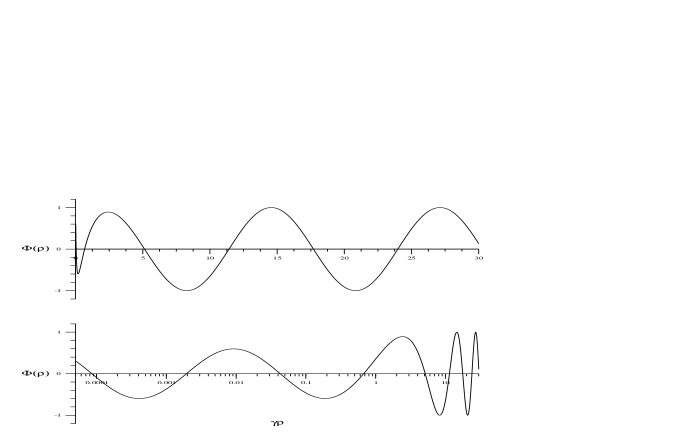
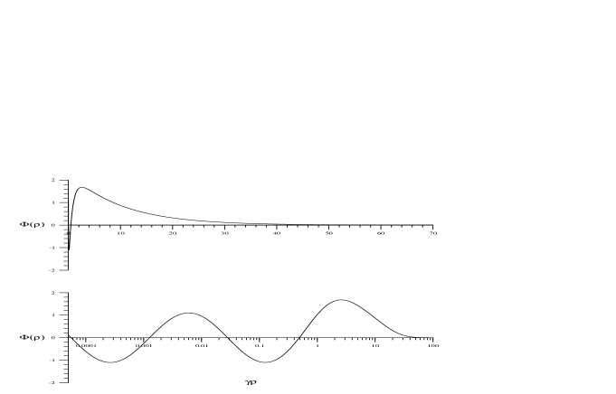
Figure 6.1: Numerical 2+1 scattering solution to eqn. (6.27) with relative momenta $k_{0}=\gamma/2$ and total centre of mass energy $E=-13\gamma^{2}/(16M)$

Figure 6.2: Numerical solution to eqn. (6.27). Example of a shallow bound state solution with centre of mass energy $E=-101\gamma^{2}/(100M)$.

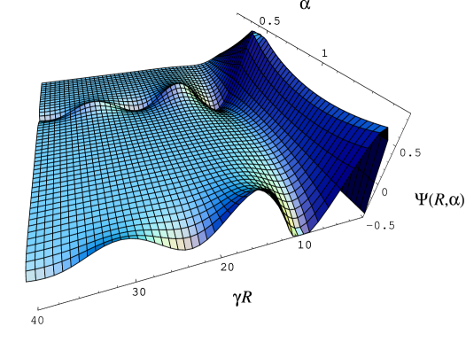
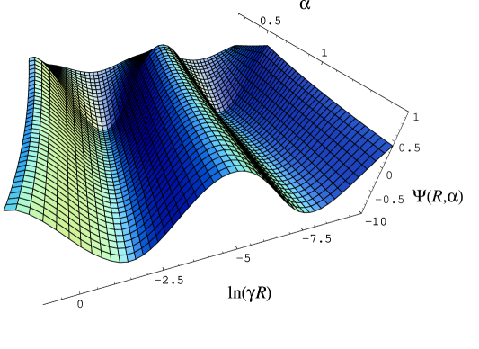
Figure 6.3: Three-body distorted wave, numerical solution to eqns. ( 6.26,6.27) with relative momenta $k_{0}=\gamma/2$ and total centre mass energy $E=-13\gamma^{2}/(16M)$.

Figure 6.4: The small $R$ detail of fig. 6.4, matching the anticipated result, eqn. (6.35).

Two sample solutions of eqn. (6.27) are shown in Figs. 6.2, 6.2. Fig. 6.2 shows a scattering solution to the equation with incoming momenta $k_{0}=\gamma/2$. The figure shows the solution on both log and linear plots so that the interior and exterior behaviour of the wavefunction is visible. In the interior the trig-log behaviour is evident, externally the solution goes to $\sin(k_{0}y+\delta)$ where $\delta$ is the phaseshift for the elastic scattering amplitude. The full DW, $\Psi(x,y)$ which results from this solution and was obtained using eqn. (6.26) is shown in Figs. 6.4,6.4.

The full DW solution is plotted on a hyperpolar scale $(R,\alpha)$. The hyperradius $R$ can be considered the mean distance between the particles and the hyperangle $\alpha$ describes the configuration of the three particles. Evident in the plots is the symmetry of the wavefunction with respect to the interchange of particles. In the fig. 6.4 the hyperradial scale is linear. There are two outgoing states at $\alpha=\pi/2$, corresponding to the ‘chosen’ bound pair, and at $\alpha=\pi/6$ corresponding to the other two possible pairs. The discontinuity across the derivative at $\alpha=\pi/6$, anticipated in eqn. (6.35) is also evident. Fig. 6.4 shows the small $R$ detail of the DWs, which exactly matches the analytic result, (6.35).

Fig. 6.2 shows a bound state solution to eqn. (6.27), again showing detail on both log and linear plots. The interior phase of this solution was determined by the choice of binding energy. From an EFT perspective the three-body force determines the interior phase which in turn determines the binding energy.

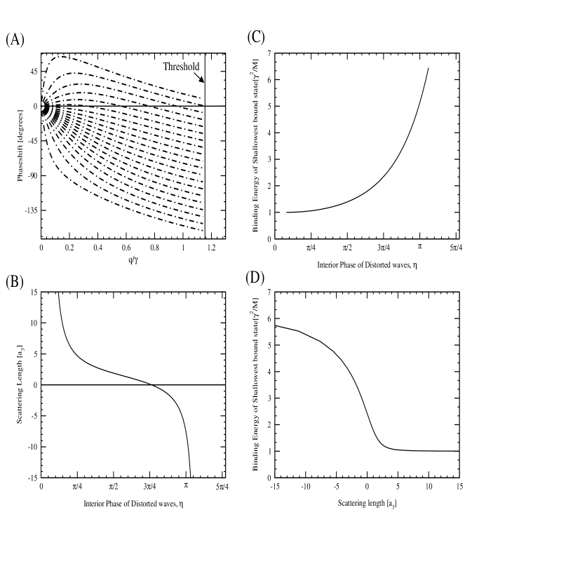
Figure 6.5: Numerical Results of the LO EFT for three-bosons. (A) All possible phaseshift curves that result from different values of the leading three body force. Each value for the LO three body force corresponds to a different interior phase $\eta$ and results in a different scattering length for 2+1 elastic scattering (B) and the shallowest bound state (C). Together these imply a single parameter relationship between the scattering length and binding energy of the bound states (D).

Fig. 6.5 shows physical observables determined from solutions to the LO EFT equation (6.27). Fig. 6.5(A) shows the possible different phaseshift curves for the elastic amplitude that result from different choices for the LO three-body force. Each of these curves corresponds to a different value for the scattering length (Fig. 6.5(B)). The range of possible scattering lengths that can be obtained from different three-body forces is $-\infty<a_{3}<\infty$. Notice that it is only because the three-body force occurs at such a low order, $(Q/\Lambda_{0})^{0}$ that it is able to affect the scattering length of these amplitudes so completely. Fig. 6.5(C) shows the shallowest bound states that result from our choice of three-body force. Figs. 6.5(B) and 6.5(C) together imply that there is a single parameter relationship between the elastic scattering length and the binding energy of the shallowest bound state, which is illustrated in Fig. 6.5(D). This curve cannot be seen experimentally as the physical world corresponds to just one point on it. However, the equivalent curve in the three nucleon problem, known as the Phillips line [22, 24, 61] has very interesting implications.

6.1.5 NLO Equations

At NLO, $(Q/\Lambda_{0})^{1}$, in accordance with eqn. (5.76) there is no extra three-body force term but there is an effective range correction in the two-body force. The equations for the effective range corrections can be found using eqn. (6.14) and the form for the two-body $T$-matrix with effective range corrections,

$$\displaystyle{\tau(p,k)=-\frac{4\pi}{M}\frac{1}{-\gamma+\frac{1}{2}\rho_{e}\left(\gamma^{2}+p^{2}-\frac{3}{4}k^{2}\right)+\sqrt{\frac{3}{4}k^{2}-p^{2}}}}$$

$$\displaystyle{\qquad\,\,\,\,\,\,\,=\frac{4\pi}{M}\frac{1}{\gamma^{2}-\frac{3}{4}k^{2}+p^{2}}\Biggl{[}\left(\gamma+\sqrt{\frac{3}{4}k^{2}-p^{2}}\right)}$$

$$\displaystyle{\qquad\qquad\qquad\qquad\qquad\qquad\qquad+\frac{1}{2}\rho_{e}\left(\gamma+\sqrt{\frac{3}{4}k^{2}-p^{2}}\right)^{2}+\ldots\Biggr{]}.}$$ (6.49)

This modified form of the effective range expansion ensures that there is a bound state pole at $i\gamma$. Substituted into eqn. (6.14) and keeping just terms of order $(Q/\Lambda_{0})$ (i.e. neglecting terms like $\rho_{e}^{2}$) gives,

$$\displaystyle{\left(k_{0}^{2}-k^{2}\right)\Phi({\bf k})-\Biggl{[}\frac{16\pi}{3M}\left(\gamma+\sqrt{\frac{3}{4}k^{2}-p^{2}}\right)}$$

$$\displaystyle{\qquad\qquad+\frac{8\pi}{3M}\rho_{e}\left(\gamma+\sqrt{\frac{3}{4}k^{2}-p^{2})}\right)^{2}\Biggr{]}\int\frac{{\rm d}^{3}{\bf k^{\prime}}}{(2\pi)^{3}}L_{2}(p,{\bf k,k^{\prime}},0)\Phi({\bf k^{\prime}})=0.}$$ (6.50)

Fourier transforming this equation as before we obtain,

$$\left(\nabla^{2}+k_{0}^{2}\right)\Phi({\bf y})+\int{\rm d}^{3}{\bf y^{\prime}}\bigl{(}V_{0}({\bf y,y^{\prime}})+\rho_{e}V_{1}({\bf y,y^{\prime}})\bigr{)}\Phi({\bf y^{\prime}})=0,$$ (6.51)

where (see Appendix E),

$$\displaystyle{V_{1}(y,y^{\prime})=-\frac{8\pi}{3M}\int\frac{{\rm d}^{3}{\bf k}}{(2\pi)^{3}}\int\frac{{\rm d}^{3}{\bf k^{\prime}}}{(2\pi)^{3}}\left[\gamma+\sqrt{\frac{3}{4}k^{2}-p^{2}}\right]^{2}L_{2}(p,{\bf k,k^{\prime}},0)e^{i({\bf k.y-\bf k^{\prime}.y^{\prime}})}}$$

$$\displaystyle{\qquad\,\,\,\,\,\,\,\,\,\,=\frac{\sqrt{3}\kappa^{2}}{2\pi^{2}}\Biggl{\{}\frac{3\kappa^{2}y^{\prime 2}}{8}\frac{K_{4}(\kappa{\cal R})}{{\cal R}^{4}}+\kappa\left(\gamma y^{\prime}-\frac{3}{2}\right)\frac{K_{3}(\kappa{\cal R})}{{\cal R}^{3}}}$$

$$\displaystyle{\qquad\qquad\qquad\qquad\qquad\qquad\qquad\qquad\qquad+\frac{2\gamma}{3}\left(\gamma-\frac{2}{y^{\prime}}\right)\frac{K_{2}(\kappa{\cal R})}{{\cal R}^{2}}\Biggr{\}}.}$$ (6.52)

The s-wave equivalent follows quite simply,

$$\left(\frac{{\rm d}^{2}}{{\rm d}y^{2}}+k_{0}^{2}\right)\Phi(y)+\int_{0}^{\infty}{\rm d}y^{\prime}(v_{0}(y,y^{\prime})+\rho_{e}v_{1}(y,y^{\prime})\Phi(y^{\prime})=0,$$ (6.53)

where

$$\displaystyle{v_{1}(y,y^{\prime})=\frac{2\sqrt{3}\kappa}{\pi}\Biggl{\{}\frac{3\kappa^{2}y^{\prime 2}}{8}\left(\frac{K_{3}(\kappa R_{-})}{R_{-}^{3}}-\frac{K_{3}(\kappa R_{+})}{R_{+}^{3}}\right)+\kappa\left(\gamma y^{\prime}-\frac{3}{2}\right)\left(\frac{K_{2}(\kappa R_{-})}{R_{-}^{2}}-\frac{K_{2}(\kappa R_{+})}{R_{+}^{2}}\right)}$$

$$\displaystyle{\qquad\qquad\qquad\qquad\qquad\qquad+\frac{2\gamma}{3}\left(\gamma-\frac{2}{y^{\prime}}\right)\left(\frac{K_{1}(\kappa R_{-})}{R_{-}}-\frac{K_{1}(\kappa R_{+})}{R_{+}}\right)\Biggr{\}}.}$$ (6.54)

We can solve eqn. (6.53) up to order $\rho_{e}$ using first order perturbation theory. If we define $\Phi(y)=\Phi^{(0)}(y)+\rho_{e}\Phi^{(1)}(y)$ and $\Phi^{(0)}(y)$ satisfies the LO equation (6.27) then up to order $\rho_{e}$, $\Phi^{(1)}(y)$ satisfies

$$\left(\frac{{\rm d}^{2}}{{\rm d}y^{2}}+k_{0}^{2}\right)\Phi^{(1)}(y)+\int_{0}^{\infty}{\rm d}y^{\prime}v_{0}(y,y^{\prime})\Phi^{(1)}(y^{\prime})=-\int_{0}^{\infty}v_{1}(y,y^{\prime})\Phi^{(0)}(y^{\prime}).$$ (6.55)

This equation may be solved numerically by adapting the method used for the LO equation. Since no new parameters are entered at this order the results of solving the equations to this order give a refinement to the one parameter relationship between the 2+1 scattering length and the three particle binding energies.

6.2 The Pionless EFT for Three Nucleons.

One area where the two-body EFT for short range forces has proven very successful is nuclear physics. As noted in the earlier chapters, nuclear physics provides an excellent and physically important example of the KSW power-counting scheme in action. In this chapter we will extend the results of the previous section to look at the pionless KSW EFT for three nucleons.

The spin and isospin degrees of freedom available to the nucleons as well as Fermi statistics makes the problem slightly more complicated then the analysis for Bosons. To avoid the complication of electromagnetic interactions we shall concentrate on the system of two neutrons and a proton.

If the total spin of the three nucleons is $3/2$ then the three spins are aligned and the Pauli exclusion principle acts as a repulsive force between the two neutrons. This system is insensitive to short range physics and has been successfully described by an EFT without three-body forces [66]. However, if the total spin is $1/2$ then, because it is possible for the three nucleons, now non-identical, to approach each other, the system is sensitive to short range physics, it is upon this system that we shall concentrate in this chapter.

6.2.1 Wavefunction Symmetry

We assume that the pairwise nuclear force conserves both isospin and spin so that these may be taken as constants, and we put the total spin and isospin and isospin component to $S=T=T_{z}=\frac{1}{2}$. If we identify one particular pair of nucleons, $1$ and $2$, then we can identify two linearly independent states of three particles with spin $1/2$ that may be used as a basis. Firstly, the singlet state in which the pair of nucleons are in the spin singlet state, $s=0$, which we denote by $\omega_{s}^{12}$ and secondly, the triplet state in which the pair are in a spin triplet state, $s=1$, which we denote by $\omega_{t}^{12}$. The singlet state is antisymmetric and the triplet state is symmetric under interchange of $1$ and $2$. A spin basis may also be constructed using an alternative pair, $2$ and $3$ say, as the starting point for the basis. The transformations between the different possible bases are given by,

$$\left(\begin{array}[]{c}\omega^{23}_{s}\\ \omega^{23}_{t}\end{array}\right)=\left(\begin{array}[]{cc}-\frac{1}{2}&-\frac{\sqrt{3}}{2}\\ -\frac{\sqrt{3}}{2}&-\frac{1}{2}\end{array}\right)\left(\begin{array}[]{c}\omega^{12}_{s}\\ \omega^{12}_{t}\end{array}\right)\qquad\left(\begin{array}[]{c}\omega^{31}_{s}\\ \omega^{31}_{t}\end{array}\right)=\left(\begin{array}[]{cc}-\frac{1}{2}&\frac{\sqrt{3}}{2}\\ \frac{\sqrt{3}}{2}&-\frac{1}{2}\end{array}\right)\left(\begin{array}[]{c}\omega^{12}_{s}\\ \omega^{12}_{t}\end{array}\right).$$ (6.56)

Similarly for isospin we have the singlet and triplet states, $\vartheta_{s}^{12}$ and $\vartheta_{t}^{12}$ which satisfy the same transformations and symmetries.

Since the pairwise potential is symmetric under interchange of the two interacting particles the continuous part of the wavefunction must be symmetric under interchange of the particles in the pair. Thus a general state which is antisymmetric in $1$ and $2$ can be written in the form,

$$|\varphi^{12}\rangle\rangle=\omega_{s}^{12}\vartheta_{t}^{12}|\psi_{s}^{12}\rangle+\omega_{t}^{12}\vartheta_{s}^{12}|\psi_{t}^{12}\rangle.$$ (6.57)

The full wavefunction, which must be antisymmetric in the interchange of any pair can now be written as,

$$|\Psi\rangle\rangle=|\varphi^{12}\rangle\rangle+|\varphi^{23}\rangle\rangle+|\varphi^{31}\rangle\rangle=(1+P)|\varphi\rangle\rangle,$$ (6.58)

where $P$ is the permutation operator. To see that $|\Psi\rangle\rangle$ is totally antisymmetric notice that

$$|\varphi^{23}\rangle\rangle\rightarrow|\varphi^{13}\rangle\rangle=-|\varphi^{31}\rangle\rangle,$$ (6.59)

under the interchange of $1$ and $2$. Since we have now introduced the permutation operator, $P$, we shall drop particle labels. Using the decomposition of $|\Psi\rangle\rangle$ we can write down the Faddeev equation for $|\varphi\rangle\rangle$,

$$(H_{0}+\hat{V}-E)|\varphi\rangle\rangle=-\hat{V}P|\varphi\rangle\rangle,$$ (6.60)

where the hat on the potential signifies that it is an operator in spin-isospin space.

We shall assume that the potential $\hat{V}$ is diagonal in spin and isospin. (This assumption is approximate but is true to the orders at which we shall be working [22].) In the centre of mass frame of the two interacting particles the Pauli exclusion principle restricts $\hat{V}$ to just two non-zero matrix elements:

$$(\omega_{s}\vartheta_{t},\hat{V}\omega_{s}\vartheta_{t})=V_{s},\qquad(\omega_{t}\vartheta_{s},\hat{V}\omega_{t}\vartheta_{s})=V_{t}.$$ (6.61)

The matrix elements, in spin-isospin space, of $\hat{V}P$ now follow from the transformation relationships (6.56),

$$(\omega_{s}\vartheta_{t},\hat{V}P\omega_{s}\vartheta_{t})=\frac{1}{4}V_{s}P,$$

$$(\omega_{s}\vartheta_{t},\hat{V}P\omega_{t}\vartheta_{s})=\frac{3}{4}V_{s}P,$$

$$(\omega_{t}\vartheta_{s},\hat{V}P\omega_{t}\vartheta_{s})=\frac{1}{4}V_{t}P,$$

$$(\omega_{t}\vartheta_{s},\hat{V}P\omega_{s}\vartheta_{t})=\frac{3}{4}V_{t}P.$$ (6.62)

Taking the inner product of eqn. (6.60) with $\omega_{s}\vartheta_{t}$ and $\omega_{t}\vartheta_{s}$ yields coupled Faddeev equations for the $|\psi_{s}\rangle$ and $|\psi_{t}\rangle$,

$$(H_{0}+V_{s}-E)|\psi_{s}\rangle=-V_{s}P\left(\frac{1}{4}|\psi_{s}\rangle+\frac{3}{4}|\psi_{t}\rangle\right),$$

$$(H_{0}+V_{t}-E)|\psi_{t}\rangle=-V_{t}P\left(\frac{3}{4}|\psi_{s}\rangle+\frac{1}{4}|\psi_{t}\rangle\right),$$ (6.63)

which can be written in the form,

$$\displaystyle{|\psi_{s}\rangle=G_{0}^{+}(E)t_{s}(E)P\left(\frac{1}{4}|\psi_{s}\rangle+\frac{3}{4}|\psi_{t}\rangle\right),}$$

$$\displaystyle{|\psi_{t}\rangle=|\chi_{t}\rangle+G_{0}^{+}(E)t_{t}(E)P\left(\frac{3}{4}|\psi_{s}\rangle+\frac{1}{4}|\psi_{t}\rangle\right),}$$ (6.64)

where $|\chi_{t}\rangle$ is the asymptotic state with a bound pair (the deuteron) and free particle. There is no bound pair in the singlet channel so there is no asymptotic state.

Using eqns. (6.56,6.58) we can now write the full wavefunction in its final form,

$$\displaystyle{|\Psi\rangle\rangle=\omega_{s}\vartheta_{t}|\Psi_{s}\rangle+\omega_{t}\vartheta_{s}|\Psi_{t}\rangle+(\omega_{s}\vartheta_{s}-\omega_{t}\vartheta_{t})|\Psi_{u}\rangle},$$

$$\displaystyle{\qquad\qquad|\Psi_{s}\rangle=\left(1+\frac{P}{4}\right)|\psi_{s}\rangle+\frac{3P}{4}|\psi_{t}\rangle,}$$

$$\displaystyle{\qquad\qquad|\Psi_{t}\rangle=\left(1+\frac{P}{4}\right)|\psi_{t}\rangle+\frac{3P}{4}|\psi_{s}\rangle,}$$

$$\displaystyle{\qquad\qquad|\Psi_{u}\rangle=\frac{\sqrt{3}}{4}\tilde{P}(|\psi_{s}\rangle+|\psi_{t}\rangle),}$$ (6.65)

where, $\langle{\bf x}_{12},{\bf y}_{3}|\tilde{P}=\langle{\bf x}_{23},{\bf y}_{1}|-\langle{\bf x}_{31},{\bf y}_{2}|$. From these equations we may now parallel the analysis for three Bosons to obtain the equations for the full wavefunction which are,

$$\displaystyle{\Psi_{a}({\bf k,x})=-\frac{4\pi}{M}\int\frac{{\rm d}^{3}{\bf k^{\prime}}}{(2\pi)^{3}}\left[L_{1}(p,{\bf k,k^{\prime},x})\Phi_{a}({\bf k^{\prime}})+L_{2}(p,{\bf k,k^{\prime},x})\left\{\frac{1}{4}\Phi_{a}({\bf k^{\prime}})+\frac{3}{4}\Phi_{b}({\bf k^{\prime}})\right\}\right],}$$

$$\displaystyle{\qquad\qquad\,\,\,\,\,\Psi_{u}({\bf k,x})=-\frac{\sqrt{3}\pi}{M}\int\frac{{\rm d}^{3}{\bf k^{\prime}}}{(2\pi)^{3}}L_{3}(p,{\bf k,k^{\prime},x})\Bigl{[}\Phi_{s}({\bf k^{\prime}})+\Phi_{t}({\bf k^{\prime}})\Bigr{]},}$$

$$\displaystyle{\qquad\qquad\tau_{a}\left(p,k\right)^{-1}\Phi_{a}({\bf k})=\int\frac{{\rm d}^{3}{\bf k^{\prime}}}{(2\pi)^{3}}L_{2}(p,{\bf k,k^{\prime}},0)\left[\frac{1}{4}\Phi_{a}({\bf k^{\prime}})+\frac{3}{4}\Phi_{b}({\bf k^{\prime}})\right],}$$ (6.66)

where $a,b\in\{s,t\}$ with $a\neq b$, and $L_{3}$ is given by,

$$L_{3}(p,{\bf k,k^{\prime},x})=-2iM\frac{\sin[{{\bf x}}.({\bf k^{\prime}}+\frac{1}{2}{\bf k})]}{k^{2}+k^{\prime 2}+{\bf k.k^{\prime}}-p^{2}-i\epsilon}.$$ (6.67)

6.2.2 The Coordinate Space Equations.

These equations can as before be readily converted into coordinate space. The equations for $\Psi({\bf x},{\bf y})$ do not depend upon the two-body $T$-matrices and are given by,

$$\displaystyle{\Psi_{a}({\bf x},{\bf y})=\int d^{3}y^{\prime}\left[W_{1}({\bf y},{\bf y}^{\prime},{\bf x})\Phi_{a}({\bf y}^{\prime})+W_{2}({\bf y},{\bf y}^{\prime},{\bf x})\left(\frac{1}{4}\Phi_{a}({\bf y}^{\prime})+\frac{3}{4}\Phi_{b}({\bf y}^{\prime})\right)\right],}$$ (6.68)

$$\displaystyle{\qquad\qquad\Psi_{u}({\bf x},{\bf y})=\int d^{3}y^{\prime}W_{3}({\bf y},{\bf y}^{\prime},{\bf x})\left(\frac{1}{4}\Phi_{a}({\bf y}^{\prime})+\frac{3}{4}\Phi_{b}({\bf y}^{\prime})\right),}$$ (6.69)

where

$$\displaystyle{\qquad\,\,\,\,W_{1}({\bf y},{\bf y}^{\prime},{\bf x})=\frac{\sqrt{3}\kappa^{2}}{4\pi^{2}}\frac{K_{2}(\kappa{\cal Q}_{0})}{{\cal Q}_{0}^{2}},}$$ (6.70)

$$\displaystyle{W_{2}({\bf y},{\bf y}^{\prime},{\bf x})=\frac{\sqrt{3}\kappa^{2}}{4\pi^{2}}\left\{\frac{K_{2}(\kappa{\cal Q}_{+})}{{\cal Q}_{+}^{2}}+\frac{K_{2}(\kappa{\cal Q}_{-})}{{\cal Q}_{-}^{2}}\right),}$$ (6.71)

$$\displaystyle{W_{3}({\bf y},{\bf y}^{\prime},{\bf x})=\frac{3\kappa^{2}}{16\pi^{2}}\left\{\frac{K_{2}(\kappa{\cal Q}_{+})}{{\cal Q}_{+}^{2}}-\frac{K_{2}(\kappa{\cal Q}_{-})}{{\cal Q}_{-}^{2}}\right).}$$ (6.72)

In order to get the equations for $\Phi(y)$ we must define the two-body $T$-matrices. The $T$-matrix in the triplet channel is given by,

$$\displaystyle{\tau_{t}(p,k)=-\frac{4\pi}{M}\frac{1}{-\gamma_{t}+\frac{1}{2}\rho_{t}\left(\gamma_{t}^{2}+p^{2}-\frac{3}{4}k^{2}\right)+\sqrt{\frac{3}{4}k^{2}-p^{2}}}}$$

$$\displaystyle{\qquad\,\,\,\,\,\,\,=\frac{4\pi}{M}\frac{1}{\gamma_{t}^{2}-\frac{3}{4}k^{2}+p^{2}}\Biggl{[}\left(\gamma_{t}+\sqrt{\frac{3}{4}k^{2}-p^{2}}\right)}$$

$$\displaystyle{\qquad\qquad\qquad\qquad\qquad\qquad\qquad+\frac{1}{2}\rho_{t}\left(\gamma_{t}+\sqrt{\frac{3}{4}k^{2}-p^{2}}\right)^{2}+\ldots\Biggr{]}.}$$ (6.73)

This has a pole at $p=i\gamma_{t}$, which corresponds to the deuteron, hence $\gamma_{t}$ is given by the deuteron binding momenta $\gamma_{t}=45.70$MeV. The effective range is $\rho_{t}=1.764$fm. In the singlet channel there is no bound state so the $T$-matrix is given by,

$$\displaystyle{\tau_{s}(p,k)=-\frac{4\pi}{M}\frac{1}{-\gamma_{s}+\frac{1}{2}r_{s}\left(p^{2}-\frac{3}{4}k^{2}\right)+\sqrt{\frac{3}{4}k^{2}-p^{2}}}}$$

$$\displaystyle{\qquad\,\,\,\,\,\,\,=\frac{4\pi}{M}\frac{1}{\gamma_{s}^{2}-\frac{3}{4}k^{2}+p^{2}}\Biggl{[}\left(\gamma_{s}+\sqrt{\frac{3}{4}k^{2}-p^{2}}\right)}$$

$$\displaystyle{\qquad\qquad\qquad+\frac{1}{2}r_{s}\left\{\left(\gamma_{s}+\sqrt{\frac{3}{4}k^{2}-p^{2}}\right)^{2}-\gamma_{s}^{2}\frac{\gamma_{s}+\sqrt{\frac{3}{4}k^{2}-p^{2}}}{\gamma_{s}-\sqrt{\frac{3}{4}k^{2}-p^{2}}}\right\}+\ldots\Biggr{]}.}$$ (6.74)

The difference in the expansion makes the NLO term slightly more complicated. Here we have $\gamma_{s}^{-1}=a_{s}=-23.714$fm and $r_{s}=2.73$fm. The Fourier transforms now follow in much the same way as in the Boson case. We get,

$$\displaystyle{\left(\nabla^{2}+\frac{4}{3}\gamma_{a}^{2}-\kappa^{2}\right)\Phi_{a}({\bf y})+\int{\rm d}^{3}{\bf y^{\prime}}\Biggl{(}V_{0}^{a}({\bf y,y^{\prime}})}$$

$$\displaystyle{\qquad\qquad\qquad+r_{a}(V_{1}^{a}({\bf y,y^{\prime}})+\delta_{as}\tilde{V}_{1}^{s}({\bf y,y^{\prime}})\Biggr{)}\left(\frac{1}{4}\Phi_{a}({\bf y^{\prime}})+\frac{3}{4}\Phi_{b}({\bf y^{\prime}}\right)=0,}$$ (6.75)

where $V^{a}_{0}({\bf y},{\bf y}^{\prime})$ is given by eqn. (6.1.2) with the substitution $\gamma\rightarrow\gamma_{a}$, $V^{a}_{1}({\bf y},{\bf y}^{\prime})$ is given by eqn. (6.1.5) with the substitution $\gamma\rightarrow\gamma_{a}$ and

$$\tilde{V}^{s}_{1}(y,y^{\prime})=\frac{8\pi\gamma_{s}^{2}}{3M}\int\frac{{\rm d}^{3}{\bf k}}{(2\pi)^{3}}\int\frac{{\rm d}^{3}{\bf k^{\prime}}}{(2\pi)^{3}}\left[\frac{\gamma_{s}+\sqrt{\frac{3}{4}(k^{2}+\kappa^{2})}}{\gamma_{s}-\sqrt{\frac{3}{4}(k^{2}+\kappa^{2})}}\right]L_{2}(p,{\bf k,k^{\prime}},0)e^{i({\bf k.y-\bf k^{\prime}.y^{\prime}})}.$$ (6.76)

We were unable to evaluate this final integral analytically. It can be reduced to a one dimensional equation as in appendix E and then evaluated numerically. The s-wave equivalents of these follow easily. The term in eqn. (6.76) is neglected by Bedaque et al [24], who simply use the modified form of the ERE in the singlet channel and take $\rho_{s}=r_{s}$. The difference is comparable to NNLO corrections.

6.2.3 Analytic Results.

It is useful to rewrite the equations for $\Phi_{s}$ and $\Phi_{t}$ in terms of $\Phi_{\pm}=\Phi_{s}\pm\Phi_{t}$. The LO s-wave equations for these are then given by,

$$\displaystyle{\left(\frac{\partial^{2}}{\partial y^{2}}+\frac{2}{3}\left(\gamma_{s}^{2}+\gamma_{t}^{2}\right)-\kappa^{2}\right)\Phi_{\pm}(y)+\frac{2}{3}\left(\gamma_{s}^{2}-\gamma_{t}^{2}\right)\Phi_{\mp}(y)}$$

$$\displaystyle{\qquad\qquad\qquad\qquad+\int_{0}^{\infty}dy^{\prime}\left(v_{0}^{\pm}(y,y^{\prime})\Phi_{+}(y^{\prime})-\frac{1}{2}v_{0}^{\mp}(y,y^{\prime})\Phi_{-}(y^{\prime})\right)=0,}$$ (6.77)

where,

$$v_{0}^{\pm}(y,y^{\prime})=\frac{1}{2}(v_{0}^{s}(y,y^{\prime})\pm v_{0}^{t}(y,y^{\prime})).$$ (6.78)

The equations for $\Phi_{\pm}$ are useful because at small $y$ they decouple to give

$$\frac{{\rm d}^{2}\Phi_{\pm}(y)}{{\rm d}y^{2}}+\frac{16y\lambda_{\pm}}{\sqrt{3}\pi}\int_{0}^{\infty}{\rm d}y^{\prime}\Phi_{\pm}(y^{\prime})\frac{2y^{\prime 4}+2y^{2}y^{\prime 2}-y^{4}}{(y^{4}+y^{2}y^{\prime 2}+y^{\prime 4})^{2}}=0,$$ (6.79)

where $\lambda_{+}=1$ and $\lambda_{-}=-1/2$. Substituting $\Phi_{\pm}=y^{s}$ as before we obtain the equation for $s$,

$$\cos\left(\frac{\pi s}{2}\right)-\frac{8\lambda_{\pm}}{\sqrt{3}s}\sin\left(\frac{\pi s}{6}\right)=0.$$ (6.80)

This equation for $s$ when $\lambda=1$ is the same as the equation that describes the Bosonic wavefunction at short distances and hence has the imaginary solutions $s=\pm\bar{s}_{0}$ [25, 22, 24]. The equation for $\lambda=-1/2$ only has real solutions, the smallest of which is $s=2$. In solving eqn. (6.77) generally we may identify solutions by their behaviour at small $y$. There are solutions in which the interior behaviour is determined by a boundary condition on $\Phi_{+}(y)$, for example,

$$\displaystyle{\qquad\Phi_{+}(y)\rightarrow\sin(\bar{s}_{0}\ln\gamma_{t}y+\eta)+\ldots,}$$ (6.81)

$$\displaystyle{\Phi_{-}(y)\rightarrow{\cal A}(\gamma_{s}-\gamma_{t})\sin(\bar{\ln}\gamma_{t}y+\eta+\sigma)+\ldots,}$$ (6.82)

where the constants ${\cal A}$ and $\sigma$ can be determined by solving eqn. (6.77) order-by-order in $y$. There are also solutions in which the interior behaviour is determined by a boundary condition on $\Phi_{-}(y)$, e.g.

$$\displaystyle{\qquad\Phi_{-}(y)\rightarrow y^{2}+\ldots,}$$ (6.83)

$$\displaystyle{\Phi_{+}(y)\rightarrow{\cal B}(\gamma_{s}-\gamma_{t})y^{3}+\ldots.}$$ (6.84)

These solutions must be uniquely combined in a manner determined by the boundary conditions at $y\rightarrow\infty$. All the physical distorted waves will be dominated at short distances by the trig-log behaviour of the $\Phi_{+}$ solution.

The three-body force will prove to be very important in this system. The 3BDWRG analysis for the three Boson EFT may be extended to this example and its conclusions are very much the same. Namely the LO three-body force will be marginal and will correspond to a self-adjoint extension of the Hamiltonian. It will in effect fix the phase of the distorted waves close to the origin. The next three-body force term that can be determined occurs at the order $(Q/\Lambda_{0})^{2}$. The eqns. (6.77) plus a phase fixing condition correspond to an EFT to order $(Q/\Lambda^{0})^{0}$.

At large $y$, below the three-body threshold but above the deuteron binding energy, the singlet solution should vanish. This constitutes an additional boundary condition on the equation that determines the combination of solutions described above. After applying this boundary condition, the triplet wavefunction has the long-distance form,

$$\Phi_{t}(y)\rightarrow\sin(k_{0}y+\delta),$$ (6.85)

where $k_{0}^{2}=4/3\gamma_{t}^{2}+\kappa^{2}$ is the momentum of the free neutron in the centre of mass frame and $\delta$ is the phaseshift for neutron-deuteron scattering

In solving the NLO equations no new three-body force term is required. The $\gamma_{t},\gamma_{s}$ dependent terms at this order in the three-body force will appear as refinements in the LO ‘phase-fixing’ three-body force. At this order there are two equations to solve, corresponding to the perturbations, $r_{s}$ and $\rho_{t}$. Writing,

$$\Phi_{\pm}(y)=\Phi_{\pm}^{(0)}(y)+(r_{s}+\rho_{t})\Phi_{\pm}^{(1+)}+(r_{s}-\rho_{t})\Phi_{\pm}^{(1-)}+\ldots,$$ (6.86)

where $\Phi_{\pm}^{(0)}$ satisfy eqn. (6.77), using first order perturbation theory we obtain the equations,

$$\displaystyle{\left(\frac{\partial^{2}}{\partial y^{2}}+\frac{2}{3}\left(\gamma_{s}^{2}+\gamma_{t}^{2}\right)-\kappa^{2}\right)\Phi_{\pm}^{(1+)}(y)+\frac{2}{3}\left(\gamma_{s}^{2}-\gamma_{t}^{2}\right)\Phi_{\mp}^{(1+)}(y)}$$

$$\displaystyle{\qquad\qquad\qquad+\int_{0}^{\infty}dy^{\prime}\left(v_{0}^{\pm}(y,y^{\prime})\Phi_{+}^{(1+)}(y^{\prime})-\frac{1}{2}v_{0}^{\mp}(y,y^{\prime})\Phi_{-}^{(1+)}(y^{\prime})\right)=}$$

$$\displaystyle{\qquad\qquad\qquad\qquad\qquad\qquad-\int_{0}^{\infty}\left(v_{1}^{+}(y,y^{\prime})\Phi_{+}^{(0)}(y^{\prime})-\frac{1}{2}v_{1}^{-}(y,y^{\prime})\Phi_{-}^{(0)}(y^{\prime})\right),}$$ (6.87)

$$\displaystyle{\left(\frac{\partial^{2}}{\partial y^{2}}+\frac{2}{3}\left(\gamma_{s}^{2}+\gamma_{t}^{2}\right)-\kappa^{2}\right)\Phi_{\pm}^{(1-)}(y)+\frac{2}{3}\left(\gamma_{s}^{2}-\gamma_{t}^{2}\right)\Phi_{\mp}^{(1-)}(y)}$$

$$\displaystyle{\qquad\qquad\qquad+\int_{0}^{\infty}dy^{\prime}\left(v_{0}^{\pm}(y,y^{\prime})\Phi_{+}^{(1-)}(y^{\prime})-\frac{1}{2}v_{0}^{\mp}(y,y^{\prime})\Phi_{-}^{(1-)}(y^{\prime})\right)=}$$

$$\displaystyle{\qquad\qquad\qquad\qquad\qquad\qquad-\int_{0}^{\infty}\left(v_{1}^{-}(y,y^{\prime})\Phi_{+}^{(0)}(y^{\prime})-\frac{1}{2}v_{1}^{+}(y,y^{\prime})\Phi_{-}^{(0)}(y^{\prime})\right),}$$ (6.88)

where,

$$v_{1}^{\pm}=(v_{1}^{s}\pm v_{1}^{t}+\tilde{v}_{1}^{s})/4.$$ (6.89)

Taking $\kappa$ and $\gamma$ to zero in these equations gives equations for the behaviour of the corrections for small $y$. Since these equations become scale free at small $y$ it means that the two corrections $\Phi_{\pm}^{(1\pm)}(y)\sim y^{s-1}$ as $y$ becomes small. Hence, these ‘corrections’ radically change the form of the wavefunctions at small $y$ but provide only minor corrections at large $y$.

6.2.4 Numerical Results

We take the mass of each nucleon to the be isospin averaged mass, $M=938.9$MeV. Eqn. (6.77) may be solved numerically using a method adapted from that used in the three Boson example. To set the interior phase defined by the LO three-body force, we apply a cut-off, $\Omega$, that allows us to ‘feed’ the desired phase into the equation. Below the cut-off, $y<\Omega$, we use the form given in eqns. (6.81,6.82), for $y>\Omega$ the solution is to be determined from the resulting homogeneous equation. In order to set the exterior boundary condition on the singlet solution we must also solve eqn. (6.77) to obtain a solution that has the small $y$ asymptotic form given by eqn. (6.83).

Numerically, the solutions are again most easily found using linear algebra. The discretisation of the $y$ variable is done as before, however, since we are solving coupled equations, the matrix equation to be solved is now of order $2n$.

At NLO, the numerical solution of eqns. (6.87,6.88) is achieved similarly but is more complicated. Since these equations are still differential equations they require boundary conditions. The correct boundary conditions are those that remove all solutions to the homogeneous equations, which are identical to the LO equations. That is, the solutions of the NLO equations should be the particular integral. To find these boundary conditions we must solve eqns. (6.87,6.88) order-by-order in $y$. The results give,

$$\Phi_{+}^{(1+)}\rightarrow{\cal A}_{+}^{+}y^{-1}\sin(\bar{s}_{0}\ln y\gamma+\eta+\sigma_{+}^{+}),$$ (6.90)

$$\Phi_{-}^{(1+)}\rightarrow{\cal A}_{-}^{+}y^{-1}\sin(\bar{s}_{0}\ln y\gamma+\eta+\sigma_{-}^{+}),$$ (6.91)

$$\Phi_{-}^{(1-)}\rightarrow{\cal A}_{-}^{-}(\gamma_{s}-\gamma_{t})\sin(\bar{s}_{0}\ln y\gamma+\eta+\sigma_{-}^{-}),$$ (6.92)

$$\Phi_{+}^{(1-)}\rightarrow{\cal A}_{+}^{-}(\gamma_{s}-\gamma_{t})\sin(\bar{s}_{0}\ln y\gamma+\eta+\sigma_{+}^{-}),$$ (6.93)

where the exact values of the constants ${\cal A}$ and $\sigma$ are not important for this discussion. These boundary conditions are now fed into the equation by using the cut-off $\Omega$.

Fig. 6.6 shows the projection of the wavefunction, $\Phi(y)$, of an elastic scattering wavefunction at LO and NLO. The solid lines show the triplet wavefunction and dashed lines show the singlet wavefunction. The LO result is shown in red and the NLO result in black. Since there is no outgoing bound state in the singlet state, the singlet wavefunction vanishes as $y\rightarrow\infty$. The wave in the triplet channel corresponds to an outgoing/incoming deuteron and neutron. At small $y$ the trig-log behaviour is apparent in the LO solution. The NLO solution also displays this behaviour with an extra factor of $y^{-1}$. The LO and NLO solutions become distinct at around $2{\rm fm}\sim r_{s},\rho_{t}$.

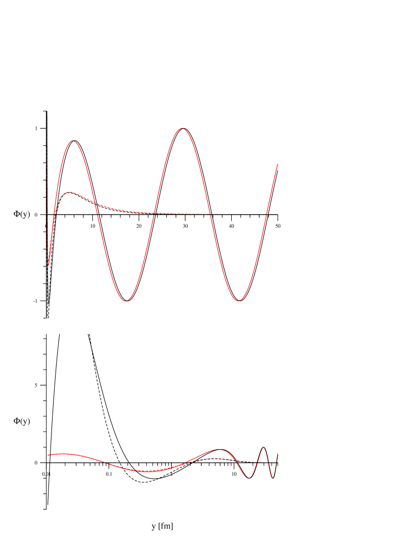
Figure 6.6: Scattering solution to eqn. (6.75) with $q_{0}=51.0$MeV ($\kappa=13.6$MeV) at LO (red) and NLO (black). The solid lines are the triplet wavefunction $\Phi_{t}(y)$, the dashed lines are the singlet wavefunction $\Phi_{s}(y)$

To obtain physical variables, the LO three-body force must be fixed. This can be done by matching to the deuteron neutron scattering length, $a_{nd}=0.65\pm 0.04$fm[63]. With this single input the EFT becomes predictive for all other scattering observables including the triton binding energy. The three-body force at NLO will differ from the three-body force at LO by a term of order $\rho_{e}\gamma$.

The relationship between the choice of three-body force, the neutron-deuteron scattering length and the triton binding energy is shown in figs. 6.8,6.8 and 6.9. Fig. 6.8 shows the values of the neutron deuteron scattering length that correspond to different interior phases of the DWs and hence to different three-body forces. Fig.6.8 shows how the binding energy of the Triton (the shallowest bound state) depends upon our choice of three body force. Many of these shallowest bound states actually lie outside the validity of the EFT defined by the pion mass.

Bringing the results of figs. 6.8 and 6.8 together gives a one variable relationship between the neutron-deuteron scattering length and the triton binding energy, fig. 6.9. Although this curve cannot be seen experimentally as the physical values correspond to a single point in this space, shown by a cross, it does have interesting implications for the study of three nucleon problems with potential models. The dots in fig. 6.9 correspond to different predictions for the triton binding energy and the neutron-deuteron scattering length obtained from different pair wise nucleon potentials with the same two body scattering lengths and effective ranges as inputs [52]. Instead of clustering randomly around the physical values, these form a curve through the space.. This relationship was first noted by Phillips [61] in looking at the predictions for three-body variables by nuclear pairwise potential models. In fig. 6.9 the NLO result (dashed) is a clear improvement upon the LO result (solid). The connection between the Phillips line and the three-body force in the three-body EFT has already been illustrated by Bedaque et al [24], our NLO curve differs slightly from theirs because of the additional term 6.76.

Figure 6.7: Neutron-Deuteron scattering lengths that result from choice of LO three-body force, corresponding to a different interior phase, $\eta$, for the trig-log behaviour of the wavefunctions. The solid and dashed lines show the LO and NLO results respectively

Figure 6.8: Triton binding energies that result from different choices of the LO three-body force. The solid and dashed lines show the LO and NLO results respectively

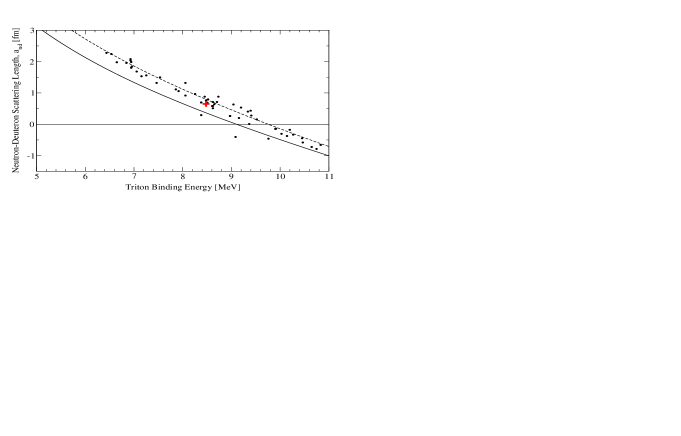
Figure 6.9: The Phillips line as predicted by the pionless EFT at LO (bold line) and NLO (dashed line). The dots correspond to the predictions for the triton binding energy and neutron-deuteron scattering length in different models with the same two-body inputs [52]. The cross is the experimental result.

	LO	NLO	Physical
Interior Phase of DWs, $\eta$, where
$\Phi\rightarrow\sin(\bar{s}_{0}\ln{\mu y}+\eta)$	2.442	2.419
and $\mu=100$MeV.
Triton Binding Energy	8.08MeV	8.68MeV	8.48MeV

Table 6.1: The interior phase of the DWs and the Triton binding energy at LO and NLO found by matching to the neutron-deuteron scattering length.

The interior phase of the DWs and the prediction for the Triton binding energy are shown in table 6.1. Fig. 6.10 shows the projection of the triton wavefunction at LO and NLO. The full LO Triton wavefunction obtained from eqn. (6.68) are shown in fig. 6.11 on hyperpolar plots. The configuration of the three particles, parameterised in $\alpha$, depends upon our choice of pair in defining $\alpha$. In the triplet wavefunction, the ‘chosen’ pair have isospin 0 and so correspond to a neutron and proton, in the singlet wavefunction the ‘chosen‘ pair are the two neutrons.

The highest value of the wavefunction occurs as a proton and neutron are paired with a second neutron around 1fm away, which occurs at $\alpha=\pi/6$, $R=1$fm in both the singlet and triplet wavefunctions and also at $\alpha=\pi/2$, $R=1$fm in the triplet wavefunction. This configuration also allows the three nucleons to be spread over the greatest volume, i.e the highest density at large values of $R$ corresponds to the values $\alpha=\pi/6$ in both singlet and triplet states and also to $\alpha=0$ in the triplet state. For $R<1$fm the wavefunction does not distinguish much between the different configurations of the three particles (different $\alpha$’s) except for $\alpha\rightarrow 0$ where the wavefunction vanishes. This value, $\alpha=0$, corresponds to the situation where the third nucleon is directly between the other two.

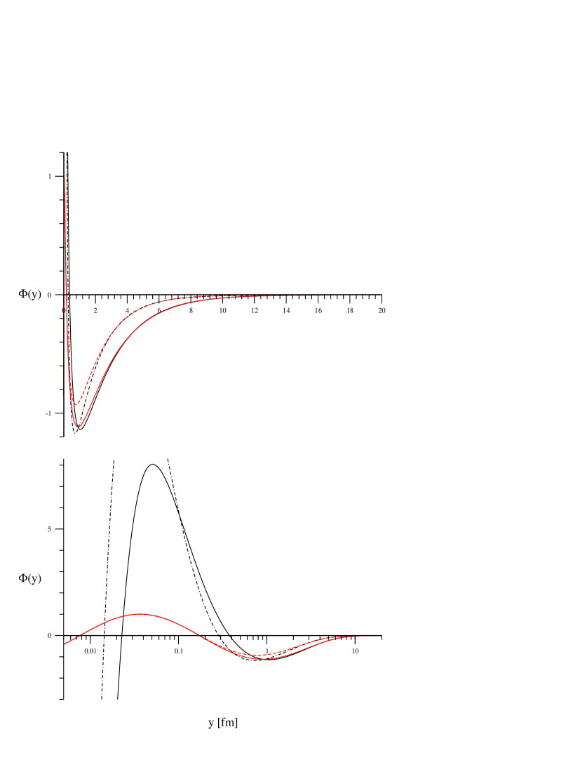
Figure 6.10: The triton wavefunction’s projection $\Phi(y)$ as found by matching the three-body force to the neutron-deuteron scattering length at LO (red) and NLO (black). The solid lines are the triplet wavefunction $\Phi_{t}(y)$, the dashed lines are the singlet wavefunction $\Phi_{s}(y)$

Singlet state $\Psi_{s}(R,\alpha)$

$\alpha$

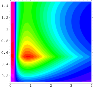
R [fm]

Triplet state $\Psi_{t}(R,\alpha)$

$\alpha$

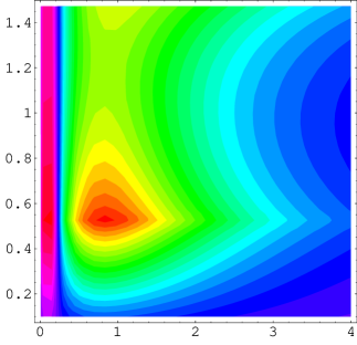
R [fm]

Figure 6.11: Contour plots showing the triton wavefunction at LO. The highest particle density occurs at $\alpha=\pi/6$, $R\sim 1$fm in both the triplet and singlet wavefunctions. This corresponds to a proton and a neutron on top of each other with the third neutron 1fm away. In the triplet wavefunction the $\alpha=\pi/2$ ‘tail’ is longer and peaks higher as this also corresponds to a proton neutron pair with a distinct neutron.

Fig. 6.12 shows the predictions for the elastic neutron-deuteron phaseshift after matching the three-body force to the neutron-deuteron scattering length at LO (solid line) and NLO (dashed line). The circles show the most recent experimental results (circa 1967) [64] and the triangles show the results obtained from a combination of V18 and Urbana IX two and three-body forces [62]. Given the age of the experimental results, in makes sense to compare the data to that obtained from sophisticated potential models, rather than the experimental data. These models are fitted to many different variables in two- and three-body systems and can be expected to produce a reasonable curve [66, 24, 33].

The EFT curve fits the potential model curve well at NLO. The computing effort in solving the EFT equations for the wavefunctions and the physical variables is minimal compared with the effort required for the more sophisticated approaches.

To go to higher orders than NLO requires considerably more effort. A new three-body force is required, isospin symmetry violation must be considered and the computational effort in calculating the four second-order perturbations is considerable. However, the agreement achieved with very few parameters and at the relatively low order of $(Q/\Lambda_{0})^{1}$ is pleasing.

Figure 6.12: Physical phaseshifts for neutron-deuteron scattering ($q_{0}=\sqrt{4/3\gamma_{t}^{2}-\kappa^{2}}$) with the LO three-body force fitted to the neutron-deuteron scattering length. The solid and dashed lines are the LO and NLO result respectively. The circles are the most recent experimental results from 1967[64] and the triangles are the results obtained using the Argonne V18+Urbana IX two and three-body forces [62].

6.2.5 Summary

In this chapter we have derived and solved equations for the three body DWs for three Bosons and three nucleons at LO and NLO in the KSW EFT. In each case a ‘phase-fixing’ three-body force is required.

The implications of the LO three-body force in the case of three nucleons is embodied in the Phillip’s line, which shows the one parameter relation between the neutron-deuteron scattering length and the triton binding energy as predicted by pairwise nuclear potentials. The NLO results show convergence upon the potential model results in both the neutron-deuteron phaseshift and the Phillip’s line.

The equations, once the three-body force is determined by fitting to the neutron-deuteron scattering length, yield the triton wavefunction and all DWs describing elastic scattering of a neutron and a deuteron below breakup. The triton wavefunction result can be used in applications, such as electron triton scattering.

Chapter 7 Conclusions

In this thesis we have looked at the use of the renormalisation group in the development of effective field theories. Our three main results are the development of a tool, the DWRG and general methods of solving the DWRG equation; the use of the 3BDWRG equation in deriving the limit-cycle solution for the three-body force in the KSW EFT for short-range forces and the corresponding power-counting; the development and solution of equations that can be used to practically evaluate three body DWs in the KSW EFT for Bosons and the physically and mathematically interesting system of three nucleons in the ${}^{3}S_{1}$ channel.

The DWRG is tool that enables us to resum some diagrams to all orders. The general method of solving the DWRG equation relies upon the basic loop integral, perturbations about which give an alternate power-counting scheme to naive dimensional analysis that corresponds to a trivial fixed point in the DWRG. What is pleasing about the results we have obtained, using the DWRG, is that established results such as the DWERE for well-behaved potentials share a common method with new results such as the limit-cycle solutions for short range forces with an attractive inverse square potential.

The solution of the DWRG for the attractive inverse square problem required a little care. The system is not properly defined without the input of a scale, $p_{0}$, that defines a self-adjoint extension. The solutions of the DWRG are in the form of limit-cycles. The power-counting associated with the limit-cycle solutions have a LO marginal term, which corresponds to the degree of freedom offered by the choice of $p_{0}$. The solution of the DWRG answers many issues raised in refs. [30, 32] concerning the connection between the short range effective force and the need for a self-adjoint extension, the possibility of multi-valued solutions of the RG, and the lack of a ground state.

Our study of the KSW EFT three-body problem was motivated by the recent realisation that the three-body force is extremely important in some systems [22, 24]. Two systems that are particularly interesting are the three s-wave Bosons and three nucleons in the ${}^{3}S_{1}$ channel. These systems have no net repulsion due to the pair-wise forces and result in singularities similar to the attractive inverse square potential. Because of this similarity, the 3BDWRG solutions exhibit limit-cycle behaviour and a three-body force that occurs at order $(Q/\Lambda_{0})^{0}$. Our results confirm the power-counting proposed by Bedaque et al [22, 24]. The power of our approach is that we are able to give a simple algebraic statement of that counting.

Our results also illustrate the limit cycle behaviour of the three-body force that has been suggested based on analysis of the attractive inverse square potential [30, 32] and the STM equation [22, 24].

The generalisation of the 3BDWRG to four or more bodies is straightforward, our method of solution involving the basic loop integral is easily generalised. The scale-free systems studied in this thesis and the novel power-counting schemes that correspond to them are likely to be important in N-body forces in the KSW EFT due to the scale-free nature of these systems at hyperradii far smaller than the two-body scattering length.

The final chapter offers some physical results for the KSW EFT. The convergence of the results using a limit-cycle three-body force and their agreement with the results of sophisticated potential methods has already been shown, [24, 33]. To complement these results and to offer new possibilities of testing the EFT we have derived equations that allow calculation of the DWs for the three-body KSW EFT below threshold. Our equations are the coordinate space equivalent of the STM equations [56]. Taking advantage of what we had shown earlier, the LO three-body force can be chosen by simply fixing the phase of the DWs at small hyperradii.

Our results for three nucleons in the ${}^{1}S_{1}$ channel agree well with those of Bedaque et al (up to a difference in definition of NLO corrections). Our method allows us to calculate particle density of the triton wavefunction that may be tested by looking at electron-triton scattering data.

In summary, the DWRG has shown itself to be a versatile tool and has been used to shed light on several issues currently under debate. This thesis has produced several results that provide insight into current issues in the EFT community and open new doors for testing the KSW EFT for short-range forces.

Appendix A Analyticity of $\hat{J}(\hat{p},\hat{\kappa})$

We want to study the analyticity of the integral,

$$I=\int_{0}^{1}d\hat{q}{\cal C}(\hat{\kappa}/\hat{q})=2\pi\kappa\int_{0}^{1}\frac{d\hat{q}}{\hat{q}(e^{\frac{2\pi\kappa}{\hat{q}}}-1),}$$ (A.1)

which we can write as,

$$I=2\pi\hat{\kappa}\int_{2\pi\hat{\kappa}}^{\infty}\frac{dx}{x(e^{x}-1)}=2\pi A\hat{\kappa}-\int^{2\pi\hat{\kappa}}\frac{dx}{x(e^{x}-1)},$$ (A.2)

where $A$ is some constant. Since we are investigating the behaviour of the integral near $\hat{\kappa}\rightarrow 0$ we can expand the integrand in the final term in a series in $x$ and assume $\kappa$ to be within the radius of convergence to get,

$$I=2\pi A\hat{\kappa}-\int^{2\pi\hat{\kappa}}dx\left(\frac{1}{x^{2}}-\frac{1}{2x}+\frac{1}{12}+\ldots\right)=1+\pi\hat{\kappa}\bigl{(}2A+\ln\hat{\kappa}+\ln 2\pi\bigr{)}-\frac{\pi\hat{\kappa}}{6}+\ldots.$$ (A.3)

Appendix B DWRG Analysis for the Attractive Coulomb Potential

In this appendix we shall look quickly at the modifications to the DWRG analysis for an attractive Coulomb potential, i.e. when $\kappa$ is negative.

Clearly, the power-counting around each fixed point is unchanged as these result from the form of the DWRG equation rather than details. The trivial fixed point is also unchanged, the expansion around it yields the distorted wave Born expansion, eqn. (3.31).

The two differences that result from having an attractive Coulomb potential is the existence of bound states that occur in the truncated Green’s function and the definition of the non-trivial fixed point. In the repulsive case the starting point for the non-trivial fixed point solution was the basic loop integral,

$$\hat{J}(\hat{p},\hat{\kappa})=\fint_{0}^{1}\hat{q}^{2}d\hat{q}\frac{{\cal C}(\hat{\kappa}/\hat{q})}{\hat{p}^{2}-\hat{q}^{2}}.$$ (B.1)

However, in the repulsive case this integral no longer converges because of the essential singularity at $\hat{q}=0$. To remedy this, we now define $\hat{J}$ as

$$\hat{J}(\hat{p},\hat{\kappa})=\text{Re}\int_{c}\hat{q}^{2}d\hat{q}\frac{{\cal C}(\hat{\kappa}/\hat{q})}{\hat{p}^{2}-\hat{q}^{2}},$$ (B.2)

where $c$ is the contour shown in fig. B.1. This integral is convergent because it approaches the essential singularity from the other direction.

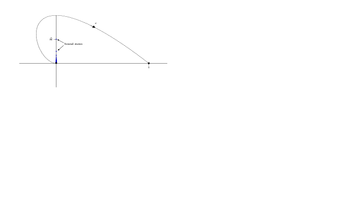
Figure B.1: The contour of integration in the complex $\hat{q}$-plane for the non-trivial fixed point in the attractive Coulomb case. The bound states appear as poles at $\hat{q}=i\hat{\kappa}/n$.

The integral $\hat{J}$ can now be split up as before to isolate the singularities:

$$\displaystyle{\hat{J}(\hat{p},\hat{\kappa})=-\text{Re}\int_{c}d\hat{q}\,{\cal C}(\hat{\kappa}/\hat{q})-\hat{p}^{2}\int_{1}^{\infty}d\hat{q}\frac{{\cal C}(\hat{\kappa}/\hat{q})}{\hat{p}^{2}-\hat{q}^{2}}+\hat{\cal M}(\hat{p},\hat{\kappa}),}$$ (B.3)

$$\displaystyle{\qquad\qquad\qquad\hat{\cal M}(\hat{p},\hat{\kappa})=\hat{p}^{2}\,\text{Re}\int_{c^{\prime}}d\hat{q}\frac{{\cal C}(\hat{\kappa}/\hat{q})}{\hat{p}^{2}-\hat{q}^{2}}},$$ (B.4)

where the contour $c^{\prime}$ extends the contour $c$ along the real axis to infinity. As in the repulsive case, the second term is analytic, the term $\hat{\cal}M$ is not analytic but satisfies the homogeneous DWRG equation and the first term contains logarithmic dependence, which is still given by the analysis in the previous appendix. Hence we can write the non-trivial fixed point solution precisely as before,

$$\hat{V}_{S}^{(0)}=\Bigl{(}\hat{J}(\hat{p}\hat{\kappa})-\hat{\cal M}(\hat{p},\hat{\kappa})-\hat{\cal L}(\hat{\kappa},\Lambda)\Bigr{)}^{-1}.$$ (B.5)

where ${\cal L}$ is defined in eqn. (3.39). Now we have found a non-trivial fixed point solution the comments on the RG flow are the same as in the repulsive case.

We will find that when writing down the distorted wave effective range expansion there is the additional bound state terms in the truncated Green’s function. Eqn. (3.47) should now read,

$$\frac{\langle\psi_{p}|\tilde{K}_{S}|\psi_{p}\rangle}{|\psi_{p}(R)|^{2}}=V_{S}(p,\kappa,\Lambda)\left(1-V_{S}(p,\kappa,\Lambda)\left\{\frac{M}{2\pi^{2}}\fint_{0}^{\Lambda}dq\frac{|\psi_{q}(R)|^{2}}{p^{2}-q^{2}}+\frac{M}{4\pi}\sum_{n=1}^{\infty}\frac{|\psi_{n}(R)|^{2}}{p^{2}+p_{n}^{2}}\right\}\right)^{-1},$$ (B.6)

where $\psi_{n}(r)$ is the bound state with binding energy $E_{n}=|\kappa|^{2}/n^{2}$ and is given by,

$$\psi_{n}(r)=\sqrt{\frac{\kappa^{3}}{n^{5}}}2re^{-\kappa r/n}L_{n-1}^{1}(2\kappa r/n)\rightarrow 2r\left(\frac{\kappa}{n}\right)^{3}\text{as $r\rightarrow 0$},$$ (B.7)

where $L^{\alpha}_{n}$ is the associated Laguerre Polynomial. The term in braces in eqn. (B.6) may be written as,

$$\frac{M\Lambda R^{2}}{2\pi^{2}}\left(\int_{0}^{1}d\hat{q}\frac{\hat{q}^{2}{\cal C}(\hat{\kappa}/\hat{q})}{\hat{p}^{2}-\hat{q}^{2}}-\sum_{n=1}^{\infty}{\cal R}\left\{\frac{\hat{q}^{2}{\cal C}(\hat{\kappa}/\hat{q})}{\hat{p}^{2}-\hat{q}^{2}},\hat{q}\rightarrow i|\kappa|/n\right\}\right)$$ (B.8)

and so by Cauchy’s theorem is equal to $M\Lambda^{2}\hat{J}(\hat{p},\hat{\kappa})$. The analysis follows as before, resulting in the DWERE,

$${\cal C}(\eta)\cot\tilde{\delta}_{S}-{\cal M}(p,\kappa)=-2\kappa\ln{\frac{\kappa}{\mu}}-\frac{2\Lambda_{0}}{\pi}\sum_{n,m}\hat{C}_{2n,m}\left(\frac{p^{2n}\kappa^{m}}{\Lambda_{0}^{2n+m}}\right),$$ (B.9)

where,

$$\displaystyle{{\cal M}(p,\kappa)=\frac{2\Lambda}{\pi}\hat{\cal M}(\hat{p},\hat{\kappa})=\text{Re}\int_{c}^{\prime}\frac{dq}{q}\frac{4\kappa}{e^{2\pi\kappa/q}-1}\frac{p^{2}}{p^{2}-q^{2}}}$$

$$\displaystyle{\qquad\qquad\qquad\qquad\qquad\qquad=-2\kappa\text{Re}\left[\ln(-i\eta)+\frac{1}{2i\eta}-\psi(-i\eta)\right].}$$ (B.10)

Appendix C The Faddeev Equations for Three Identical Bosons

For a system with three particles the Lippmann-Schwinger equation is inadequate. Although the three-body $T$-matrix satisfies the Lippmann-Schwinger equation, it is not possible to use this equation to find it because its kernel is not compact. This may be understood in several ways. Most simply in coordinate space it is a result of a non-vanishing potential as the mean separation of the three particles is taken to infinity but two of the particles remain close. This in turn is related to the possibility of incoming and outgoing boundary conditions involving bound states of particles and also to the possibility of so-called disconnected diagrams, in which one of the three-particles fails to interact.

In short, a wave-function with an incoming two-body bound state and a single particle satisfies the homogeneous version of the Lippmann-Schwinger equation resulting in non-unique solutions. The resolution to this quandary is well-known. We must ensure that disconnected diagrams are not allowed. One favoured method is to use the Faddeev equations.

Consider the case of three identical bosons interacting via a pairwise interaction $V_{2B}$. The wavefunction must be symmetric with respect to transposition of any two particle indices, hence the wavefunction, $|\Psi^{+}\rangle$ with incoming boundary conditions of three free particles (rather than a bound state of any two) can be written as

$$|\Psi^{+}\rangle=|\psi_{0}\rangle+(1+P)|\psi^{+}\rangle,$$ (C.1)

where $|\psi_{0}\rangle$ is the ‘in’-state and solves the free Schrödinger equation and $P$ is a permutation operator, which permutes particle indices and has the matrix elements defined in eqn. (5.3). The Schrödinger equation is written as,

$$\displaystyle{\qquad\qquad(H_{0}+(1+P)V_{2B}-E)|\Psi^{+}\rangle=0,}$$ (C.2)

$$\displaystyle{(1+P)(H_{0}+V_{2B}-E)|\psi^{+}\rangle=-(1+P)V_{2B}(|\psi_{0}\rangle+P|\psi^{+}\rangle,}$$ (C.3)

where to obtain the second line, we have used the fact that $H_{0}$ commutes with the permutation operator, $P$. Cancelling the $(1+P)$ on the left hand side and using $G_{2B}^{+}=(E-V_{2B}-H_{0}+i\epsilon)^{-1}$ we obtain,

$$|\psi^{+}\rangle = G_{2B}^{+}(E)V_{2B}|\psi_{0}\rangle+G_{2B}^{+}(E)V_{2B}^{+}P|\psi^{+}\rangle,$$ (C.4)

$$= G_{0}^{+}(E)t^{+}(E)|\psi_{0}\rangle+G_{0}^{+}(E)t^{+}(E)P|\psi^{+}\rangle,$$ (C.5)

where $t^{+}$ is the $T$-matrix given by the equation, $t^{+}(E)=V_{2B}+V_{2B}G_{2B}^{+}(E)V_{2B}$. Eqn. (5.4) is the Faddeev equation for the wavefunction component $|\psi^{+}\rangle$. It is connected because of the $P$-operator which ensures that each interaction, given by the two-body $T$-matrix, is not between the same two particles as the preceding one.

The corresponding equations for the full three-body Green’s function and $T$-matrix now follow from similar decompositions. If we write the full $T$-matrix, $\cal T$ in terms of components,

$${\cal T^{+}}(E)=(1+P)T^{+}(E),$$ (C.6)

then from the equation defining the full wavefunction in terms of the Möller wave operator $1+G_{0}^{+}(E){\cal T^{+}}(E)$,

$$|\Psi^{+}\rangle=(1+G_{0}^{+}(E){\cal T^{+}}(E))|\psi_{0}\rangle=|\psi_{0}\rangle+(1+P)G_{0}^{+}(E)T^{+}|\psi_{0}(E)\rangle,$$ (C.7)

and from the definition of $|\Psi^{+}\rangle$ in terms of its components, eqn. (5.1), we obtain the relation, $|\psi^{+}\rangle=G_{0}^{+}(E)T^{+}(E)|\psi_{0}\rangle$, which when substituted into the Faddeev eqn. (5.4) yields the Faddeev equation for the $T$-matrix component,

$$T^{+}(E)=t^{+}(E)+t^{+}(E)G_{0}^{+}(E)PT^{+}(E).$$ (C.8)

We may find a similar relation for the full Green’s function, ${\cal G^{+}}(E)=G_{0}^{+}(E)+(1+P)G^{+}(E)$, by using the equation ${\cal G^{+}}(E)=G_{0}^{+}(E)+G_{0}^{+}(E){\cal T}^{+}(E)G_{0}^{+}(E)$.

Appendix D Momentum Dependent Perturbations in the DWRG for Three-Bodies

Momentum dependent perturbations about the limit cycle solution are found using the ansatz

$$\displaystyle{{\hat{V}}_{3B}(\hat{p},\hat{\gamma},\hat{k},\hat{k}^{\prime},\Lambda)={\hat{V}}_{3B}^{(0)}(\hat{p},\hat{\gamma},\Lambda)+C\Lambda^{\nu}\phi(\hat{p},\hat{\gamma},\Lambda),}$$ (D.1)

$$\displaystyle{\,\,\,\,\,\,\,\,\,\phi(\hat{p},\hat{\gamma},\Lambda)=k^{2n}\phi_{1}(\hat{p},\hat{\gamma},\Lambda)+\phi_{2}(\hat{p},\hat{\gamma},\Lambda),}$$ (D.2)

where $\phi_{1}$ and $\phi_{2}$ only depend upon $\Lambda$ logarithmically. Substituting this into the DWRG equation (5.68), neglecting for now the discontinuities, then linearising gives a partial differential equation for $\phi_{1}$ and $\phi_{2}$,

$$\displaystyle{\hat{k}^{2n}\left[-\Lambda\frac{\partial\phi_{1}}{\partial\Lambda}+\hat{p}\frac{\partial\phi_{1}}{\partial\hat{p}}+\hat{\gamma}\frac{\partial\phi_{1}}{\partial\hat{\gamma}}+(2n-\nu)\phi_{1}+V_{3B}^{(0)}\phi_{1}\frac{{\cal C}(\hat{\gamma},\ln\Lambda/p_{*})}{1-\hat{p}^{2}}\right]}$$

$$\displaystyle{\qquad\qquad+\left[-\Lambda\frac{\partial\phi_{2}}{\partial\Lambda}+\hat{p}\frac{\partial\phi_{2}}{\partial\hat{p}}+\hat{\gamma}\frac{\partial\phi_{2}}{\partial\hat{\gamma}}-\nu\phi_{2}+V_{3B}^{(0)}\phi_{2}\frac{2{\cal C}(\hat{\gamma},\ln\Lambda/p_{*})}{1-\hat{p}^{2}}\right]}$$

$$\displaystyle{\qquad\qquad\qquad\qquad\qquad\qquad\qquad\qquad\qquad+V_{3B}^{(0)}\phi_{1}\frac{\tilde{\cal C}(\hat{\gamma},\ln\Lambda/p_{*})}{1-\hat{p}^{2}}=0,}$$ (D.3)

where $\tilde{C}(\hat{\gamma},\ln\Lambda/p_{*})$ is given by,

$$\tilde{\cal C}\left(\hat{\gamma},\ln\frac{\Lambda}{p_{*}}\right)=-\hat{\gamma}^{2n}{\cal D}_{2}\left(\hat{\gamma},\ln\frac{\Lambda}{p_{*}}\right)+\int_{0}^{1}d\hat{k}\,\hat{k}^{2n}{\cal D}_{3}\left(\hat{k},\hat{\gamma},\ln\frac{\Lambda}{p_{*}}\right).$$ (D.4)

From the first line we obtain the RG eigenvalue $\nu=2n$ and the solution $\phi_{1}=\hat{V}_{3B}^{(0)}$. So that a with the further substitution,

$$\phi_{2}=\left[\phi_{3}\hat{V}_{3B}^{(0)}-\hat{p}^{2n}\right]\hat{V}_{3B}^{(0)}$$ (D.5)

we obtain a PDE for $\phi_{3}$,

$$-\Lambda\frac{\partial\phi_{3}}{\partial\Lambda}+\hat{p}\frac{\partial\phi_{3}}{\partial\hat{p}}+\hat{\gamma}\frac{\partial\phi_{3}}{\partial\hat{\gamma}}-2n\phi_{3}+\frac{\tilde{\cal C}(\hat{\gamma},\ln\Lambda/p_{*})-\hat{p}^{2n}{\cal C}(\hat{\gamma},\ln\Lambda/p_{*})}{1-\hat{p}^{2}}=0.$$ (D.6)

This equation should of course have discontinuities on the RHS. The solution of this PDE, including those discontinuities, is straight forward and can be reached in much the same way as the limit-cycle solution. The momentum perturbations occur at orders $2,4,6,\ldots$ at the same orders of the energy perturbations.

Appendix E Fourier Transforms

We wish to perform the Fourier transform,

$$\displaystyle{W({\bf y},{\bf y}^{\prime},{\bf x})=-\frac{4\pi}{M}\int\frac{{\rm d}^{3}{\bf k^{\prime}}}{(2\pi)^{3}}\int\frac{{\rm d}^{3}{\bf k^{\prime}}}{(2\pi)^{3}}L(p,{\bf k,k^{\prime},x})e^{i({\bf k.y-\bf k^{\prime}.y^{\prime}})}}$$

$$\displaystyle{\qquad\qquad\,\,\,=\frac{1}{x}\int\frac{d^{3}{\bf k}}{(2\pi)^{3}}e^{i{\bf k}.({\bf y-y^{\prime}})}e^{ix\sqrt{p^{2}-\frac{3}{4}k^{2}}}}$$

$$\displaystyle{\qquad\qquad\qquad+8\pi\int\frac{d^{3}{\bf k}}{(2\pi)^{3}}\int\frac{d^{3}{\bf k^{\prime}}}{(2\pi)^{3}}e^{i({\bf k.y-k^{\prime}.y^{\prime}})}\frac{\cos[{{\bf x}.({\bf k}^{\prime}+\frac{1}{2}{\bf k})}]}{k^{2}+k^{\prime 2}+{\bf k.k^{\prime}}-p^{2}-i\epsilon}.}$$ (E.1)

$$\displaystyle{\qquad\qquad\,\,\,=I_{1}+I_{2}}$$ (E.2)

Doing the integral over all angles in $I_{1}$ gives,

$$I_{1}=\frac{1}{2\pi^{2}x|{\bf y-y^{\prime}}|}\int_{0}^{\infty}dk\,k\sin(k|{\bf y-y^{\prime}}|)e^{-\frac{\sqrt{3}}{2}x\sqrt{\kappa^{2}+k^{2}}},$$ (E.3)

where we have put $\kappa=-2p/\sqrt{3}$. Using the result

$$\int_{0}^{\infty}dx\,xe^{-\beta\sqrt{\gamma^{2}+x^{2}}}\sin{bx}=\frac{\beta b\gamma^{2}}{\beta^{2}+b^{2}}K_{2}(\gamma\sqrt{\beta^{2}+b^{2}})$$ (E.4)

we get,

$$I_{1}=\frac{\sqrt{3}\kappa^{2}}{4\pi^{2}}\frac{K_{2}(\kappa{\cal Q}_{0})}{{\cal Q}_{0}^{2}}$$ (E.5)

where ${\cal Q}_{0}$ is given by eqn. (6.31). The second integral, $I_{2}$, is more involved, making the change of variable ${\bf k^{\prime\prime}}={\bf k^{\prime}+k/2}$ we obtain,

$$I_{2}=4\pi\int\frac{d^{3}{\bf k}}{(2\pi)^{3}}\int\frac{d^{3}{\bf k^{\prime\prime}}}{(2\pi)^{3}}e^{i{\bf k}.({\bf y}+\frac{1}{2}{\bf y}^{\prime})}\frac{(e^{-i{\bf k^{\prime\prime}.(y^{\prime}+x)}}+e^{-i{\bf k^{\prime\prime}.(y^{\prime}-x)}})}{k^{\prime\prime 2}+\frac{3}{4}(k^{2}+\kappa^{2})}.$$ (E.6)

Performing the ${\bf k^{\prime\prime}}$ integral gives$I_{2}=I_{+}+I_{-}$ where,

$$I_{\pm}=\frac{1}{|{\bf y^{\prime}\pm x}|}\int\frac{d^{3}{\bf k}}{(2\pi)^{3}}e^{i{\bf k}.({\bf y}+\frac{1}{2}{\bf y}^{\prime})}e^{-\frac{\sqrt{3}}{2}|{{\bf y}^{\prime}\pm{\bf x}}|\sqrt{k^{2}+\kappa^{2}}}.$$ (E.7)

Then the angular ${\bf k}$ integral can be done to give,

$$\displaystyle{I_{\pm}=\frac{1}{2\pi^{2}|{{\bf y}+\frac{1}{2}{\bf y}^{\prime}}||{{\bf y}^{\prime}\pm{\bf x}}|}\int_{0}^{\infty}dk\,k\sin(k|{{\bf y}+\frac{1}{2}{\bf y}^{\prime}}|)e^{-\frac{\sqrt{3}}{2}|{{\bf y}^{\prime}\pm{\bf x}}|\sqrt{k^{2}+\kappa^{2}}}}$$ (E.8)

$$\displaystyle{\qquad=\frac{\sqrt{3}\kappa^{2}}{4\pi^{2}}\frac{K_{2}(\kappa{\cal Q}_{\pm})}{{\cal Q}_{\pm}^{2}},}$$ (E.9)

where we have again used result (E.4). The result quoted in the text follows.

The second integral to be done is

$$\displaystyle{V_{0}({\bf y,y^{\prime}})=-\frac{16\pi}{3M}\int\frac{{\rm d}^{3}{\bf k}}{(2\pi)^{3}}\int\frac{{\rm d}^{3}{\bf k^{\prime}}}{(2\pi)^{3}}\left[\gamma+\sqrt{\frac{3}{4}k^{2}-p^{2}}\right]L_{2}(p,{\bf k,k^{\prime}},0)e^{i({\bf k.y-\bf k^{\prime}.y^{\prime}})}}$$

$$\displaystyle{\qquad\,\,\,\,\,\,\,\,\,=\frac{32\pi\gamma}{3}\int\frac{{\rm d}^{3}{\bf k}}{(2\pi)^{3}}\int\frac{{\rm d}^{3}{\bf k^{\prime}}}{(2\pi)^{3}}\frac{e^{i({\bf k.y-\bf k^{\prime}.y^{\prime}})}}{k^{2}+k^{\prime 2}+{\bf k.k^{\prime}}+\frac{3}{4}\kappa^{2}}}$$

$$\displaystyle{\qquad\qquad\qquad+\frac{16\pi}{\sqrt{3}}\int\frac{{\rm d}^{3}{\bf k}}{(2\pi)^{3}}\int\frac{{\rm d}^{3}{\bf k^{\prime}}}{(2\pi)^{3}}\sqrt{k^{2}+\kappa^{2}}\frac{e^{i({\bf k.y-\bf k^{\prime}.y^{\prime}})}}{k^{2}+k^{\prime 2}+{\bf k.k^{\prime}}+\frac{3}{4}\kappa^{2}}}$$ (E.10)

$$\displaystyle{\qquad\,\,\,\,\,\,\,\,\,=I_{3}+I_{4}.}$$ (E.11)

$I_{3}$ but for an overall numerical factor is the same of the $I_{2}$ with $x=0$. Hence we have,

$$I_{3}=\frac{2\kappa^{2}\gamma}{\sqrt{3}\pi^{2}}\frac{K_{2}(\kappa{\cal R})}{{\cal R}^{2}}.$$ (E.12)

$I_{4}$ can be done in much the same way as the $I_{2}$ integral (with $x=0$) all the way up to the final $k$ integral. Hence we get,

$$I_{4}=\frac{2}{\sqrt{3}\pi^{2}|{{\bf y}+\frac{1}{2}{\bf y}^{\prime}}|y^{\prime}}\int_{0}^{\infty}dk\,k\sqrt{k^{2}+\kappa^{2}}\sin(k|{{\bf y}+\frac{1}{2}{\bf y}^{\prime}}|)e^{-\frac{\sqrt{3}}{2}y^{\prime}\sqrt{k^{2}+\kappa^{2}}}.$$ (E.13)

Differentiating the result (E.4) on both sides w.r.t. $\beta$ gives

$$\int_{0}^{\infty}dx\,x\sqrt{\gamma^{2}+x^{2}}e^{-\beta\sqrt{\gamma^{2}+x^{2}}}\sin{bx}=\frac{\beta^{2}b\gamma^{3}}{(\beta^{2}+b^{2})^{3/2}}K_{3}(\gamma\sqrt{\beta^{2}+b^{2}})-\frac{b\gamma^{2}}{\beta^{2}+b^{2}}K_{2}(\gamma\sqrt{\beta^{2}+b^{2}}),$$ (E.14)

which can be used to obtain,

$$I_{4}=\frac{\sqrt{3}\kappa^{3}y^{\prime}}{2\pi^{2}}\frac{K_{3}(\kappa{\cal R})}{{\cal R}^{3}}-\frac{2\kappa^{2}}{\sqrt{3}y^{\prime}}\frac{K_{2}(\kappa{\cal R})}{{\cal R}^{2}}.$$ (E.15)

The quoted result follows.

The final integral is

$$\displaystyle{V_{1}({\bf y,y^{\prime}})=-\frac{8\pi}{3M}\int\frac{{\rm d}^{3}{\bf k}}{(2\pi)^{3}}\int\frac{{\rm d}^{3}{\bf k^{\prime}}}{(2\pi)^{3}}\left[\gamma+\sqrt{\frac{3}{4}k^{2}-p^{2}}\right]^{2}L_{2}(p,{\bf k,k^{\prime}},0)e^{i({\bf k.y-\bf k^{\prime}.y^{\prime}})}}$$

$$\displaystyle{\qquad\,\,\,\,\,\,\,\,\,=\frac{16\pi\gamma^{2}}{3}\int\frac{{\rm d}^{3}{\bf k}}{(2\pi)^{3}}\int\frac{{\rm d}^{3}{\bf k^{\prime}}}{(2\pi)^{3}}\frac{e^{i({\bf k.y-\bf k^{\prime}.y^{\prime}})}}{k^{2}+k^{\prime 2}+{\bf k.k^{\prime}}+\frac{3}{4}\kappa^{2}}}$$

$$\displaystyle{\qquad\qquad\qquad+\frac{16\pi\gamma}{\sqrt{3}}\int\frac{{\rm d}^{3}{\bf k}}{(2\pi)^{3}}\int\frac{{\rm d}^{3}{\bf k^{\prime}}}{(2\pi)^{3}}\sqrt{k^{2}+\kappa^{2}}\frac{e^{i({\bf k.y-\bf k^{\prime}.y^{\prime}})}}{k^{2}+k^{\prime 2}+{\bf k.k^{\prime}}+\frac{3}{4}\kappa^{2}}}$$

$$\displaystyle{\qquad\qquad\qquad\,\,\,\,\,\,4\pi\int\frac{{\rm d}^{3}{\bf k}}{(2\pi)^{3}}\int\frac{{\rm d}^{3}{\bf k^{\prime}}}{(2\pi)^{3}}(k^{2}+\kappa^{2})\frac{e^{i({\bf k.y-\bf k^{\prime}.y^{\prime}})}}{k^{2}+k^{\prime 2}+{\bf k.k^{\prime}}+\frac{3}{4}\kappa^{2}}}$$

$$\displaystyle{\qquad\,\,\,\,\,\,\,\,\,=\gamma\left(\frac{1}{2}I_{3}+I_{4}\right)+I_{5}.}$$ (E.16)

The results for $I_{3}$ and $I_{4}$ have already been established. $I_{5}$, like $I_{4}$, can be done in much the same way as the $I_{2}$ integral (with $x=0$) all the way up to the final $k$ integral. Hence we get,

$$I_{5}=\frac{1}{2\pi^{2}|{{\bf y}+\frac{1}{2}{\bf y}^{\prime}}|y^{\prime}}\int_{0}^{\infty}dk\,k(k^{2}+\kappa^{2})\sin(k|{{\bf y}+\frac{1}{2}{\bf y}^{\prime}}|)e^{-\frac{\sqrt{3}}{2}y^{\prime}\sqrt{k^{2}+\kappa^{2}}}.$$ (E.17)

Differentiating the result (E.14) on both sides w.r.t. $\beta$ gives

$$\int_{0}^{\infty}dx\,x(\gamma^{2}+x^{2})e^{-\beta\sqrt{\gamma^{2}+x^{2}}}\sin{bx}=\frac{\beta^{3}b\gamma^{4}}{(\beta^{2}+b^{2})^{2}}K_{4}(\gamma\sqrt{\beta^{2}+b^{2}})-\frac{3\beta b\gamma^{3}}{(\beta^{2}+b^{2})^{3/2}}K_{3}(\gamma\sqrt{\beta^{2}+b^{2}}),$$ (E.18)

which can be used to get,

$$I_{5}=\frac{3\sqrt{3}\kappa^{4}y^{\prime 2}}{16\pi^{2}}\frac{K_{4}(\kappa{\cal R})}{{\cal R}^{4}}-\frac{3\sqrt{3}\kappa^{3}}{4\pi^{2}}\frac{K_{3}(\kappa{\cal R})}{{\cal R}^{3}}.$$ (E.19)

All the results brought together give the result in the text.

Appendix F Zero Energy Wavefunction for the Three Body EFT

We wish to evaluate the integral

$$I=\frac{\sqrt{3}}{2\pi}\int_{0}^{\infty}{\rm d}y^{\prime}y^{\prime s}\left\{\frac{x({\mathcal{R}}_{+}^{2}-{\mathcal{R}}_{-}^{2})}{{\mathcal{R}}_{+}^{2}{\mathcal{R}}_{-}^{2}}-\frac{8}{3y^{\prime}}\log\left[\frac{{\mathcal{Q}}_{+}^{+}{\mathcal{Q}}_{-}^{-}}{{\mathcal{Q}}_{-}^{+}{\mathcal{Q}}_{+}^{-}}\right]\right\},$$ (F.1)

where,

$${\mathcal{R}}_{\pm}=\sqrt{\frac{3}{4}x^{2}+y^{2}+y^{\prime 2}\pm 2yy^{\prime}},\qquad{\mathcal{Q}}_{\pm}^{\pm}=\sqrt{\frac{3}{4}x^{2}+y^{2}+y^{\prime 2}\pm yy^{\prime}\pm\frac{3}{2}xy^{\prime}}.$$ (F.2)

In order to use residue calculus to evaluate the integral we write it as

$$\displaystyle{\qquad\qquad\qquad I=I_{1}+I_{2},}$$ (F.3)

$$\displaystyle{\,\,\,\,I_{1}=\frac{\sqrt{3}}{2\pi(1-e^{i\pi s})}\int_{-\infty}^{\infty}{\rm d}y^{\prime}y^{\prime s}\frac{x({\mathcal{R}}_{+}^{2}-{\mathcal{R}}_{-}^{2})}{{\mathcal{R}}_{+}^{2}{\mathcal{R}}_{-}^{2}},}$$ (F.4)

$$\displaystyle{I_{2}=-\frac{4}{\sqrt{3}\pi(1-e^{i\pi s})}\int_{-\infty}^{\infty}{\rm d}y^{\prime}y^{\prime s-1}\log\left[\frac{{\mathcal{Q}}_{+}^{+}{\mathcal{Q}}_{-}^{-}}{{\mathcal{Q}}_{-}^{+}{\mathcal{Q}}_{+}^{-}}\right].}$$ (F.5)

The poles of the integrand of $I_{1}$ are given by the zeroes of ${\cal R}_{\pm}$ which may be written in terms of the hyperpolar coordinates as,

$$y^{\prime}=\pm i\frac{\sqrt{3}}{2}Re^{\pm i\alpha}.$$ (F.6)

Evaluating the integral using the two residues in the upper half-plane (recalling that $0<\alpha<\pi/2$) we get,

$$I_{1}=\left(\frac{\sqrt{3}R}{2}\right)^{s}\csc\left(\frac{\pi s}{2}\right)\sin(\alpha s).$$ (F.7)

$I_{2}$ can be evaluated by closing the contour in the upper half plane then collapsing it onto the branch cuts there. The branch points are given by the zeroes of ${\cal Q}_{\pm}^{\pm}$ which are simply,

$$y^{\prime}=\frac{\sqrt{3}}{2}Re^{\pm i(\alpha\pm\pi/6)}\qquad\text{and}\qquad y^{\prime}=\frac{\sqrt{3}}{2}Re^{\pm i(\alpha\pm 5\pi/6)}.$$ (F.8)

How the branch points up are joined up depends on the value of $\alpha$. We do not want any of the branch cuts to cross the real axis. The branch structures are shown in Fig. F.1.

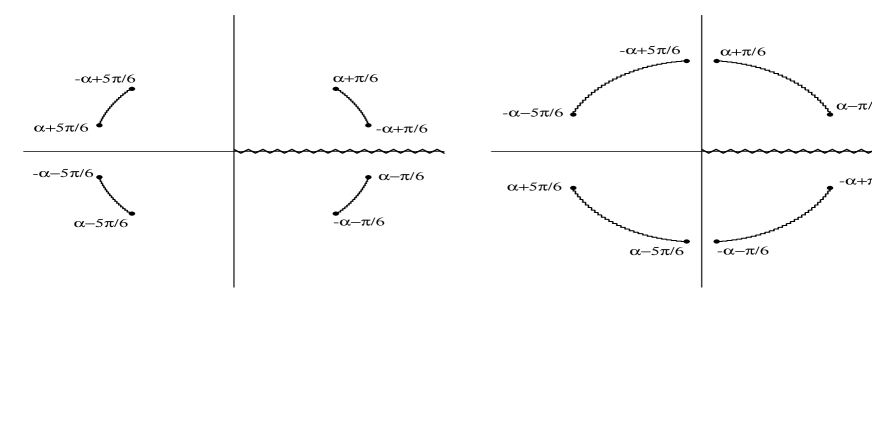
Figure F.1: The branch structure of the integrand in $I_{2}$, the labels show the argument of the branch point. On the left the case of $0<\alpha<\pi/6$ and on the right $\pi/6<\alpha<\pi/2$.

Simply evaluating the integrals around the branch cuts gives,

$$I_{2}=\begin{cases}\left(\frac{\sqrt{3}R}{2}\right)^{s}\frac{16}{s\sqrt{3}}\frac{\cos\left(\frac{\pi s}{6}\right)\sin(\alpha s)}{1+2\cos\left(\frac{\pi s}{3}\right)},&\text{when $\alpha<\frac{\pi}{6}$,}\\ \left(\frac{\sqrt{3}R}{2}\right)^{s}\frac{8}{s\sqrt{3}}\frac{\sin\left(\frac{\pi s}{2}-\alpha s\right)}{1+2\cos\left(\frac{\pi s}{3}\right)}&\text{when $\alpha>\frac{\pi}{6}$.}\end{cases}$$ (F.9)

Finally using the equation for $s$ (6.34), and combining the two results we obtain the quoted result.

Bibliography

- [1] G. Ecker, Prog. Part. Nucl. Phys. 35, 1 (1995) [hep-ph/9501357].
- [2] V. Bernard, N. Kaiser and U.-G. Meissner, Int. J. Mod. Phys. E4, 193 (1995) [hep-ph/9501384].
- [3] U. van Kolck, Prog. Part. Nucl. Phys. 43, 337 (1999) [nucl-th/9902015].
- [4] R. Seki, U. van Kolck and M. J. Savage (editors), Nuclear Physics with Effective Field Theory (World Scientific, Singapore, 1998).
- [5] P. F. Bedaque, M. J. Savage, R. Seki and U. van Kolck (editors), Nuclear Physics with Effective Field Theory II (World Scientific, Singapore, 1999).
- [6] S. R. Beane, P. F. Bedaque, W. C. Haxton, D. R. Phillips and M. J. Savage, nucl-th/0008064.
- [7] S. Weinberg, Physica A96, 327 (1979).
- [8] S. Weinberg, Phys. Lett. B251, 288 (1990); Nucl. Phys. B363, 3 (1991).
- [9] D. B. Kaplan, M. J. Savage, and M. B. Wise, Phys. Lett. B424, 390 (1998) [nucl-th/9801034]; Nucl. Phys. B534, 329 (1998) [nucl-th/9802075].
- [10] U. van Kolck, Nucl. Phys. A645, 273 (1999) [nucl-th/9808007].
- [11] J. Gegelia, nucl-th/9802038; Phys. Lett. B429, 227 (1998); J. Phys. G: Nucl. Part. Phys. 25, 1681 (1999) [nucl-th/9805008].
- [12] E. Epelbaum, W. Glöckle and U.-G. Meissner, Nucl. Phys. A637, 107 (1998); Nucl. Phys. A671, 295 (2000) [nucl-th/9910064].
- [13] S. R. Beane, T. D. Cohen and D. R. Phillips, Nucl. Phys. A632, 445 (1998) [nucl-th/9709062].
- [14] M. C. Birse, J. A. McGovern and K. G. Richardson, Phys. Lett. B464, 169 (1999) [hep-ph/9807302].
- [15] K. G. Wilson and J. G. Kogut, Phys. Rep. 12, 75 (1974); J. Polchinski, Nucl. Phys. B231, 269 (1984); R. D. Ball and R. S. Thorne, Ann. Phys. 236, 117 (1994); T. R. Morris, Prog. Theor. Phys. Suppl. 131, 395 (1998).
- [16] J. Schwinger, Phys. Rev. 72, 742A (1949).
- [17] T. Barford and M. C. Birse, Phys. Rev. C60:064006 (2003) [hep-ph/0206146].
- [18] R. G. Newton, Scattering Theory of Waves and Particles. 2nd Edition. (Springer, New York, 1982).
- [19] H. A. Bethe, Phys. Rev. 76, 38 (1949).
- [20] J. D. Jackson and J. M. Blatt, Rev. Mod. Phys. 22, 77 (1950); J. M. Blatt and J. D. Jackson, Phys. Rev. 76, 18 (1949).
- [21] X. Kong and F. Ravndal, Phys. Lett. B450, 320 (1999) [nucl-th/9811076]; Nucl. Phys. A665, 137 (2000) [hep-ph/9903523].
- [22] P. F. Bedaque, H.-W. Hammer and U. van Kolck, Phys. Rev. Lett. 82, 463 (1999) [nucl-th/9809025]; Nucl. Phys. A646, 444 (1999) [nucl-th/9811046]; Nucl. Phys. A676, 357 (2000) [nucl-th/9906032].
- [23] H.-W. Hammer and T. Mehen, Nucl. Phys. A690, 535 (2001) [nucl-th/0011024]; Phys. Lett. B516, 353 (2001) [nucl-th/0105072].
- [24] P. F. Bedaque, G. Rupak, H. W. Griesshammer and H.-W. Hammer, Nucl. Phys. A714, 589 (2003) [nucl-th/0207034]
- [25] V. N. Efimov, Sov. J. Nucl. Phys. 12, 589 (1971).
- [26] L. H. Thomas, Phys. Rev. 47, 903 (1935).
- [27] K. M. Case, Phys. Rev. 80, 797 (1950).
- [28] K. Meetz, Il Nuovo Cimento 34, 690 (1964).
- [29] A. M. Perelomov and V. S. Popov, Thoer. Math. Phys. 4, 664 (1970).
- [30] M. Bawin and S. A. Coon, [quant-ph/0302199]
- [31] H. E. Camblong and C. R. Ordóñez, [hep-th/0305035].
- [32] S. R. Beane, P. F. Bedaque, L. Childress, A. Kryjevski, J. McGuire and U. van Kolck, Phys. Rev. A64:042103, (2001) [quant-ph/0010073].
- [33] I. R. Afnan and D. R. Phillips [nucl-th/0312021]
- [34] B. Blankleider and J. Gegelia,[nucl-th/0009007].
- [35] D. R. Phillips, G. Rupak and M. J. Savage, Phys. Lett. B473, 209 (2000) [nucl-th/9908054]
- [36] J.-W. Chen, G. Rupak and M. J. Savage, Nucl. Phys. A653, 386 (1999) [nucl-th/9902056].
- [37] K. G. Richardson, Ph. D. thesis, University of Manchester (1999) [hep-ph/0008118].
- [38] T. D. Cohen and J. M. Hansen, Phys. Rev. C59, 13 (1999) [nucl-th/9808038]; Phys. Rev. C59, 3047 (1999) [nucl-th/9901065].
- [39] D. B. Kaplan and J. V. Steele, Phys. Rev. C60:064002 (1999) [nucl-th/9905027]
- [40] U. van Kolck, Nucl. Phys. A631, 56c (1998) [hep-ph/9707228].
- [41] L. S. Gradshteyn and I. M. Ryzhik, Table of Integrals, Series, and Products. 6th Edition. (Academic Press, San Diego, San Fransisco, New York, Boston, London, Sydney and Tokyo, 2000)
- [42] X. Kong and F. Ravndal, Nucl. Phys. A665, 137 (2000); Phys. Rev. C64:044002 (2001).
- [43] H. van Haeringen and L. P. Kok, Phys. Rev. A26, 1218 (1982).
- [44] D. B. Kaplan, M. J. Savage and M. B. Wise, Nucl. Phys. B478, 629 (1996) [nucl-th/9605002].
- [45] J. V. Steele and R. J. Furnstahl, Nucl. Phys. A645, 439 (1999) [nucl-th/9808022].
- [46] S. Fleming, T. Mehen and I. W. Stewart, Nucl. Phys. A677, 313 (2000) [nucl-th/9911001].
- [47] L. D. Landau and J. Smorodinski, J. Phys. Acad. Sci. USSR, 8, 219 (1944).
- [48] T. Barford and M. C. Birse, AIP Conf. Proc. 603, 229 (2001) [nucl-th/0108024].
- [49] C. Ordóñez, L. Ray and U. van Kolck, Phys. Rev. C53, 2086 (1996) [hep-ph/9511380].
- [50] D. B. Kaplan, M. J. Savage, and M. B. Wise, Phys. Rev. C59, 617 (1999) [nucl-th/9804032].
- [51] S. R. Beane, P. F. Bedaque, M. J. Savage and U. van Kolck, Nucl. Phys. A700, 377 (2002) [nucl-th/0104030].
- [52] V. N. Efimov and E. G. Tkachenko, Few-Body Systm. 4, 71 (1988).
- [53] St. D. Glazek and K. G. Wilson, Phys. Rev. D47, 4657 (1993)
- [54] St. D. Glazek and K. G. Wilson, Phys. Rev. Lett. 89:230401 (2002) [hep-ph/0203088].
- [55] A. LeClair, J. M. Roman and G. Sierra, hep-ph/0312141
- [56] G. V. Skorniakov and K. A. Ter-Martirosian, Sov. Phys. JETP 4, 648 (1957).
- [57] G. S. Danilov and V. I. Lebedev, Sov. Phys. JETP 44, 1509 (1963).
- [58] L. D. Faddeev, Mathematical Aspects of the Three-body Problem in Quantum Scattering Theory. (Steklov Math. Inst., Leningrad Publ. 69, transl. D. Davey and Co., New York, 1965)
- [59] F. Gabbiani, P. F. Bedaque and H. W. Griesshammer, Nucl. Phys. A675, 601 (2000) [nucl-th/9911034]
- [60] D. V. Fedorov and A. S. Jensen Phys. Rev. Lett. 71, 4103 (1993); Phys. Rev. A63:063608 (2001); Nucl. Phys. A697, 783 (2002).
- [61] A. C. Phillips, Nucl. Phys. A107, 209 (1968).
- [62] A. Kievsky, S. Rosati, W. Tornow and M. Viviani, Nuc. Phys. A607, 402 (1996).
- [63] W. Dilg, L. Koester and W. Nistler, Phys. Lett. B36, 208 (1971).
- [64] W. T. H. van Oers and J. D. Seagrave, Phys. Lett. B24, 562 (1967).
- [65] E. Braaten and H.-W. Hammer, Phys. Rev. Lett. 91:102002 (2003) [nucl-th/0303038].
- [66] P. F. Bedaque and U. van Kolck, Phys. Lett. B428, 221 (1998) [nucl-th/9710073]; Phys. Rev. C58, 641 (1998) [nucl-th/9802057].
- [67] F. Gabbiani, [nucl-th/0104088].
- [68] E. Braaten, H.-W. Hammer and M. Kusunoki, Phys. Rev. Lett 90: 120402 (2003) [cond-mat/0206232]; E. Braaten, H.-W. Hammer and T. Mehen, Phys. Rev. Lett. 88:040401 (2002) [cond-mat/0108380]; P. F. Bedaque, E. Braaten and H.-W. Hammer, Phys. Rev. Lett. 85, 908 (2000), [cond-mat/0002365]