Nonperturbative dynamics of scalar field theories through the Feynman-Schwinger representation

Abstract

In this paper we present a summary of results obtained for scalar field theories using the Feynman-Schwinger (FSR) approach. Specifically, scalar QED and $\chi^{2}\phi$ theories are considered. The motivation behind the applications discussed in this paper is to use the FSR method as a rigorous tool for testing the quality of commonly used approximations in field theory. Exact calculations in a quenched theory are presented for one-, two-, and three-body bound states. Results obtained indicate that some of the commonly used approximations, such as Bethe-Salpeter ladder summation for bound states and the rainbow summation for one body problems, produce significantly different results from those obtained from the FSR approach. We find that more accurate results can be obtained using other, simpler, approximation schemes.

I Introduction

In the study of hadronic physics one has to face the problem of determining the quantum dynamical properties of physical systems in which the interaction between the constituents is of a nonperturbative nature. In particular, such systems support bound states and clearly nonperturbative methods are needed to describe their properties. Assuming that such systems can be described by a field theory, one has to rely on some approximation scheme. One common approximation is known as perturbation theory. Perturbation theory involves making an expansion in the coupling strength of the interaction. The Green’s function in field theory can be expanded in powers of the coupling strength. In order to be able to obtain a bound state result one must sum the interactions to all orders. Most practical calculations to date have been done within the Bethe-Salpeter framework, where the resulting kernel is perturbatively truncated. In this paper we will discuss another method, which is based on the path integral formulation of Feynman and Schwinger Feynman (1982); Schwinger (1951). It was initiated by Simonov and collaborators Simonov (1988, 1989, 1991); Simonov, and Tjon (1993); Simonov and Tjon (2002); Simonov, Tjon and Weda (2002); Simonov, and Tjon (2002) in their study of quantum chromo-dynamics (QCD).

With the discovery of QCD, nonperturbative calculations in field theory have become even more essential. It is known that the building blocks of matter, quarks and gluons, only exist in bound states. Therefore any reaction that involves quarks will necessarily involve bound states in the initial and/or final states. This implies that even at high momentum transfers, where QCD is perturbative, formation of quarks into a bound state necessitates a nonperturbative treatment. Therefore it is essential to develop new methods for doing nonperturbative calculations in field theory.

The plan of this article is as follows. In the following section a brief review of the particle trajectory method in field theory will be given. The Feynman-Schwinger representation will be introduced through applications to scalar fields. In particular, the emphasis will be on comparing various nonperturbative results obtained by different methods. It will be shown with examples that nonperturbative calculations are interesting and exact nonperturbative results could significantly differ from those obtained by approximate nonperturbative methods.

Results for scalar quantum electrodynamics are discussed in section 3. In particular, a cancellation is found between the vertex corrections and self-energy contributions, so that the exact result can be described by essentially the sum of only the generalized exchange ladders. In section 4 the bound states are obtained for a $\chi^{2}\phi$ theory in a quenched approximation. Exact results are presented for the binding energies of two- and three-body bound states and compared with relativistic quasi-potential predictions. Section 5 deals with the stability of the $\chi^{2}\phi$ theory. It is argued that the quenched theory does not suffer from the well known instability of a $\phi^{3}$ theory. The paper closes with some concluding remarks.

II Feynman-Schwinger representation

Nonperturbative calculations can be divided into two general categories: (i) integral equations, and (ii) path integrals. Integral equations have been used for a long time to sum interactions to all orders with various approximations Salpeter, and Bethe (1951); Gross, and Milana (1991); Tiemeijer, and Tjon (1994); Savkli, and Gross (1999). In general a complete solution of field theory to all orders can be provided by an infinite set of integral equations relating vertices and propagators of the theory to each other. However solving an infinite set of equations is beyond our reach and usually integral equations are truncated by various assumptions about the interaction kernels and vertices. The most commonly used integral equations are those that deal with few-body problems. The Bethe-Salpeter equations Salpeter, and Bethe (1951) are the starting point of those investigations. Approximations schemes have extensively been studied, where in addition to solutions of the Bethe-Salpeter equation Wright, Levine, and Tjon (1967); Nakanishi (1969, 1988); Nieuwenhuis, and Tjon (1996); Savkli, and Tabakin (1998) also 3-dimensional reductions Salpeter (1952); Logunov, and Tavkhelidze (1963); Blankenbecler, and Sugar (1963); Gross (1969, 1982); Wallace, and Mandelzweig (1989) have been explored for the N-particle free particle Greens’ function. In most calculations the ladder approximation has been used for the kernel of the resulting equations. Issues of convergence of these schemes remain. Therefore it is important to have exact solutions of field theory models available to test these approximations. One promising way to reconstruct exact solutions of field theory is the path integral method.

Path integrals provide a systematic method for summing interactions to all orders. The Green’s function in field theory is given by the path integral expression:

$$\langle 0|T[\phi(x_{1})\phi(x_{2})\cdots\phi(x_{n})]|0\rangle = \frac{\biggl{\lmoustache}[{\cal D}\phi]\,\phi(x_{1})\,\phi(t_{2})\cdots\phi(x_{n})\,{\rm exp}\biggl{[}i\int d^{4}x\,L(x)\biggr{]}}{\biggl{\lmoustache}[{\cal D}\phi]\,{\rm exp}\biggl{[}i\int d^{4}x\,L(x)\biggr{]}}.$$ (1)

While path integrals provide a compact expression for the exact nonperturbative result for propagators, evaluation of the path integral is a nontrivial task.

In general, field theoretical path integrals must be evaluated by numerical integration methods, such as Monte-Carlo integration. The best known numerical integration method is lattice gauge theory. Lattice gauge theory involves a discretization of space-time and numerical integrations over field configurations are carried out using Monte-Carlo techniques. A more efficient method of performing path integrals in field theory has been proposed and it consists of explicitly integrating out the fields. It has been demonstrated to be highly successful for the case of simple scalar interactions Simonov, and Tjon (1993); Nieuwenhuis, and Tjon (1994, 1994, 1996); Savkli, Gross, and Tjon (1999, 2000); Savkli (2001); Gross, Savkli, and Tjon (2001); Savkli, Gross, and Tjon (2002); Savkli (2001). This method is known as Feynman-Schwinger representation (FSR). Through applications of the FSR, the importance of exact nonperturbative calculations will be shown with explicit examples.

The basic idea behind the FSR approach is to transform the field theoretical path integral (1) into a quantum mechanical path integral over particle trajectories. When written in terms of trajectories, the exact results decompose into separate parts, and permit us to study the individual role and numerical size of exchange, self-energy, and vertex corrections. This, in turn, alows us to study different approximations to field theory, and, in some cases. prove new results.

To illustrate these ideas, we consider the application of the FSR technique to scalar QED. The Minkowski metric expression for the scalar QED Lagrangian in Stueckelberg form is given by

$${\cal L}_{SQED} = -m^{2}\chi^{2}-\frac{1}{4}F^{2}+\frac{1}{2}\mu^{2}A^{2}$$ (2)

$$+(\partial_{\mu}-ieA_{\mu})\chi^{*}(\partial^{\mu}+ieA^{\mu})\chi$$

$$-\lambda\frac{1}{2}(\partial\cdot A)^{2}\,,$$

where $A^{\mu}$ is the gauge field of mass $\mu$, $\chi$ is the charged field of mass $m$, $F^{\mu\nu}=\partial^{\mu}A^{\nu}-\partial^{\nu}A^{\mu}$ is the gauge field tensor, and, for example, $A^{2}=A_{\mu}A^{\mu}$. The presence of a mass term for the exchange field breaks gauge invariance, and was introduced in order to avoid infrared singularities that arise when the theory is applied in 0+1 dimensions. For dimensions larger than $n=2$ the infrared singularity does not exist and therefore the limit $\mu\rightarrow~{}0$ can be safely taken to insure gauge invariance.

The path integral is to be performed in Euclidean metric. Therefore we perform a Wick rotation:

$${\rm exp}\biggl{[}i\int d^{4}x\,{\cal L}_{M}\biggr{]}\longrightarrow{\rm exp}\biggl{[}-\int d^{4}x\,{\cal L}_{E}\biggr{]}.$$ (3)

The Wick rotation for coordinates is obtained by

$$x_{0}\rightarrow-ix_{0},$$

$$\partial_{0}=\frac{\partial}{\partial x^{0}}\rightarrow i\partial_{0}\,.$$ (4)

The transformation of field $A$ under Wick rotation is found by noting that under a gauge transformation:

$$A_{\mu} \rightarrow A_{\mu}+\partial_{\mu}\Lambda\,.$$ (5)

Then, under a Wick rotation,

$$A_{0} \rightarrow iA_{0}\,,$$ (6)

and the Wick rotated Lagrangian for SQED becomes

$${\cal L}_{SQED} = \chi^{*}\biggl{[}m^{2}-\partial^{2}-2ieA\cdot\partial-ie\partial\cdot A$$ (7)

$$\qquad+e^{2}A^{2}\biggr{]}\chi+{\cal L}_{A}\,.$$

The exchange field part of the Lagrangian is given by

$${\cal L}_{A} \equiv \frac{1}{2}A_{\mu}(\mu^{2}g_{\mu\nu}-\lambda\partial_{\mu}\partial_{\nu})A_{\nu}+\frac{1}{4}F^{2}$$ (8)

$$= \frac{1}{2}A_{\mu}\Bigl{[}(\mu^{2}-\Box)g_{\mu\nu}$$

$$\qquad+(1-\lambda)\partial_{\mu}\partial_{\nu}\Bigr{]}A_{\nu}\,.$$

We employ the Feynman gauge $\lambda=1$ which yields

$${\cal L}_{A} = \frac{1}{2}A_{\nu}(\mu^{2}-\Box)A_{\nu}\,.$$ (9)

The two-body Green’s function for the transition from an initial state $\Phi_{i}(x,\bar{x})$ to final state $\Phi_{f}(y,\bar{y})$ is given by

$$G(y,\bar{y}|x,\bar{x})=N\int{\cal D}\chi^{*}\int{\cal D}\chi\int{\cal D}A\,$$

$$\times\Phi^{*}_{f}\Phi_{i}\,e^{-S_{E}},$$ (10)

where

$$S_{E}=\int d^{4}x\,\,{\cal L}_{SQED},$$ (11)

and a gauge invariant 2-body state $\Phi$ is defined by

$$\Phi(x,\bar{x}) = \chi^{*}(x)U(x,\bar{x})\chi(\bar{x}).$$ (12)

The gauge link $U(x,y)$ which insures gauge invariance of bilinear product of fields is defined by

$$U(x,y)\equiv{\rm exp}\left[-ie\int_{x}^{y}dz\,A(z)\right].$$ (13)

One can easily see that under a local gauge transformation

$$\chi(x) \rightarrow {\rm e}^{ie\Lambda(x)}\chi(x)$$

$$A_{\mu}(x) \rightarrow A_{\mu}(x)+\partial_{\mu}\Lambda(x),$$ (14)

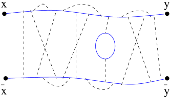
Figure 1: The dashed lines represent exchanges of the gauge field with mass $\mu$ and the solid lines the propagation of the matter fields with mass $m$. Note the matter loop in one of the middle exchanges. All loops of this kind are neglected in the quenched approximation (when $\det S=1$).

$\Phi_{i}(x,\bar{x})$ remains gauge invariant

$$\Phi(x,\bar{x}) \rightarrow {\rm exp}\biggl{[}\underbrace{-ie\Lambda(x)+ie\Lambda(\bar{x})-ie\biggl{\lmoustache}_{x}^{\bar{x}}dz_{\mu}\,\partial_{\mu}\Lambda}_{0}\biggr{]}\chi^{*}(x)U(x,\bar{x})\chi(\bar{x})=\Phi(x,\bar{x}).$$ (15)

Performing path integrals over $\chi$ and $\chi^{*}$ fields in Eq. (10) one finds

$$G(y,\bar{y}|x,\bar{x}) = N\bigg{\lmoustache}{\cal D}A\,({\rm det}S)\,\,U(x,\bar{x})U^{*}(y,\bar{y})S(x,y)S(\bar{x},\bar{y})\,e^{-S[A]}\,,$$ (16)

where the interacting 1-body propagator $S(x,y)$ is defined by

$$S(x,y) \equiv \langle y\,|\,\frac{1}{m^{2}+H(\hat{z},\hat{p})}\,|\,x\rangle$$ (17)

with

$$H(\hat{z},\hat{p}) \equiv (\hat{p}+ieA(\hat{z}))^{2}.$$ (18)

The Green’s function Eq. (16) includes contributions coming from all possible interactions. The determinant in Eq. (16) accounts for all matter ($\chi\bar{\chi}$) loops. Setting this determinant equal to unity (${\rm det}S\rightarrow 1$, referred to as the quenched approximation) eliminates all contributions from these loops (illustrated in Fig. 1) and greatly simplifies the calculation.

Analytical calculation of the path integral over the gauge field $A$ in Eq. (16) seems difficult due to the nontrivial $A$ dependence in $S(x,y)$. In more complicated theories, such as QCD, integration of the gauge field, as far as we know, cannot be done analytically. Therefore, in QCD, the only option is to do the gauge field path integral by using a brute force method. Here one usually introduces a discrete space-time lattice, and integrates over the values of the field components at each lattice site . However, for the simple scalar QED interaction under consideration, it is in fact possible to go further and eliminate the path integral over the field $A$. In order to be able to carry out the remaining path integral over the exchange field $A$ it is desirable to represent the interacting propagator in the form of an exponential. This can be achieved by using a Feynman representation for the interacting propagator. The first step involves the exponentiation of the denominator in Eq. (17):

$$S(x,y)=\int_{0}^{\infty}\!\!\!ds\,e^{-sm^{2}}\langle y|{\rm exp}[-sH]|x\rangle\,.$$ (19)

This expression is similar to a quantum mechanical propagator with $s=it$ and $H$ a Hamiltonian which is a covariant function of 4-vector momenta and coordinates. It is known how to represent a quantum mechanical propagator as a path integral. The representation is in terms of the Lagrangian, and a covariant Lagrangian can easily be obtained from the Hamiltonian (18)

Figure 2: The contour $C$, known as a Wilson loop, that arises in Eq. (24).

$$H(\hat{z},\hat{p})=(\hat{p}+ieA(\hat{z}))^{2}\,\,\Longrightarrow\,\,L(z,\dot{z})=\frac{\dot{z}^{2}}{4}-ie\,\dot{z}\cdot A(z)\,.$$ (20)

Using this Lagrangian, the path integral representation for the interacting propagator becomes

$$S(x,y) = \bigg{\lmoustache}_{0}^{\infty}ds\,\bigg{\lmoustache}\,({\cal D}z)_{xy}\,\,{\rm exp}\biggl{[}-sm^{2}-\frac{1}{4}\int_{0}^{s}d\tau_{s}\,\dot{z}^{2}(\tau_{s})-ie\int_{0}^{s}d\tau_{s}\,\dot{z}A(z(\tau_{s}))\,\,\biggr{]},$$ (21)

where $z_{i}(\tau_{s})$ is a particle trajectory which is a parametric function of the parameter $\tau_{s}$, with $s\geq\tau_{s}\geq 0$ and endpoints $z_{i}(0)=x_{i}$, $z_{i}(s)=y_{i}$, and $i=1$ to 4. This representation allows one to perform the remaining path integral over the exchange field $A$. The final result for the two-body propagator involves a quantum mechanical path integral that sums up contributions coming from all possible trajectories of the two charged particles

$$G = -\bigg{\lmoustache}_{0}^{\infty}ds\,\,\bigg{\lmoustache}_{0}^{\infty}d\bar{s}\,\,\bigg{\lmoustache}\,({\cal D}z)_{xy}\,\bigg{\lmoustache}\,({\cal D}\bar{z})_{\bar{x}\bar{y}}\,\,e^{-K[z,s]-K[\bar{z},\bar{s}]}\langle W(C)\rangle,$$ (22)

where the parameter $\tau_{s}$ is rescaled, so that $\tau_{s}=s\tau$, the kinetic term $K$ is defined by

$$K[z,s] = m^{2}s+\frac{1}{4s}\int_{0}^{1}d\tau\,\dot{z}^{2}(\tau)\,,$$ (23)

and the Wilson loop average $\langle W(C)\rangle$ is given by

$$\langle W(C)\rangle \equiv \int{\cal D}A\,{\rm exp}\biggl{[}-ie\oint_{C}dz\,A(z)-\frac{1}{2}\int d^{4}z\,A(z)(\mu^{2}-\partial^{2})A(z)\biggr{]},$$ (24)

where the contour of integration $C$ (shown in Fig. 2) follows a clockwise trajectory $x\rightarrow y\rightarrow\bar{y}\rightarrow\bar{x}\rightarrow x$ as parameters $\tau$, and $\bar{\tau}$ are varied from 0 to $1$. The $A$ integration in the definition of the Wilson loop average is of standard gaussian form and can be easily performed to obtain

$$\langle W(C)\rangle = {\rm exp}\,\biggl{[}-\frac{e^{2}}{2}\int_{C}\,dz_{\mu}\,\int_{C}\,d\bar{z}_{\nu}\,\Delta_{\mu\nu}(z-\bar{z},\mu)\biggl{]},$$ (25)

$$\Delta_{\mu\nu}(x,\mu) = g_{\mu\nu}\bigg{\lmoustache}\frac{d^{4}p}{(2\pi)^{4}}\frac{e^{ipx}}{p^{2}+\mu^{2}}\,.$$ (26)

When it is necessary to regulate the ultraviolet singularities in (26), a double Pauli-Villars subtraction will be used, so that (26) will be replaced by

$$\Delta_{\mu\nu}(x,\mu) = g_{\mu\nu}\bigg{\lmoustache}\frac{d^{4}p}{(2\pi)^{4}}\frac{e^{ipx}(\Lambda_{1}^{2}-\mu^{2})(\Lambda_{2}^{2}-\mu^{2})}{(p^{2}+\mu^{2})(p^{2}+\Lambda_{1}^{2})(p^{2}+\Lambda_{2}^{2})}\,.$$ (27)

Through the results given in Eqs. (22), (25), and either (26) or (27), the path integration expression involving fields has been transformed into a path integral representation involving trajectories of particles.

Equation (22) has a very nice physical interpretation. The term $\Delta_{\mu\nu}(z_{a}-z_{b},\mu)$ describes the propagation of gauge field interations between any two points on the particle trajectories, and the appearance of these interaction terms in the exponent means that the interactions are summed to all orders with arbitrary ordering of the points on the trajectories. Self-interactions come from terms with the two points $z_{a}$ and $z_{b}$ on the same trajectory, generalized ladder exchanges arise if the two points are on different trajectories, and vertex corrections arise from a combination of the two. Because the particles forming the two-body bound state carry opposite charges, it follows that the self energy and exchange contributions have different signs.

The bound state spectrum can be determined from the spectral decomposition of the two-body Green’s function

$$G(T)=\sum_{n=0}^{\infty}c_{n}e^{-m_{n}T},$$ (28)

where $T$ is defined as the average time between the initial and final states

$$T\equiv\frac{1}{2}(y_{4}+\bar{y}_{4}-x_{4}-\bar{x}_{4}).$$ (29)

In the limit of large $T$, the ground state mass is given by

$$m_{0}=-\lim_{T\rightarrow\infty}\frac{d}{dT}{\rm ln}[G(T)]=-\frac{\int{\cal D}ZS^{\prime}[Z]e^{-S[Z]}}{\int{\cal D}Ze^{-S[Z]}},$$ (30)

III Scalar quantum electrodynamics

In this section we take a closer look at 1-body mass pole calculations for the case of SQED. Two popular methods frequently used to find the dressed mass of a particle are to do a simple bubble summation, or to solve the 1-body Dyson-Schwinger equation in rainbow approximation. It is interesting to compare results given by the bubble summation and the Dyson-Schwinger with the exact FSR result. Below we first give a quick overview of how dressed masses can be obtained in bubble summation and the Dyson-Schwinger equation approaches. For technical simplicity, the 1-body discussion will be limited to 0+1 dimension.

The simple bubble summation involves a summation of all bubble diagrams to all orders. The dressed propagator is given by

$$\Delta_{d}(p) = \frac{1}{p^{2}+m^{2}+\Sigma(p)}.$$ (31)

The dressed mass $M$ is determined from the self energy using

$$M=\sqrt{m^{2}+\Sigma(iM)}.$$ (32)

The self energy for the simple bubble sum (in 0+1d) is given by

$$\Sigma(p) = -e^{2}\bigg{\lmoustache}_{-\infty}^{\infty}\frac{dk}{2\pi}\frac{1}{(k^{2}+\mu^{2})}$$ (33)

$$\times\bigg{\{}\frac{(2p-k)^{2}}{[(p-k)^{2}+m^{2}]}-1\bigg{\}}.$$

The self energy integral in this case is trivial and can be performed analytically, and the dressed mass is determined from Eq. (32)

The rainbow Dyson-Schwinger equation sums more diagrams than the simple bubble summation (Fig. 3). The self energy of the rainbow Dyson-Schwinger equation involves a momentum dependent mass:

$$\Sigma(p) = -e^{2}\bigg{\lmoustache}_{-\infty}^{\infty}\frac{dk}{2\pi}\frac{1}{(k^{2}+\mu^{2})}$$ (34)

$$\times \bigg{\{}\frac{(2p-k)^{2}}{[(p-k)^{2}+\underbrace{m^{2}+\Sigma(k)}]}-1\bigg{\}}\,.\qquad$$

In this case the self energy is nontrivial and it must be determined by a numerical solution of Eq. (34). The dressed mass is determined by the logarithmic derivative of the dressed propagator in coordinate space

$$M = -\lim_{T\rightarrow\infty}\frac{d}{dT}\,\,{\rm log}[\,\Delta_{d}(t)\,].$$ (35)

The type of diagrams summed by each method is shown in Fig. 3. Note that the matter loops do not give any contribution as explained earlier.

Figure 3: Various interactions included in each approach are shown.

Results obtained by these three methods are shown in Fig. 4.

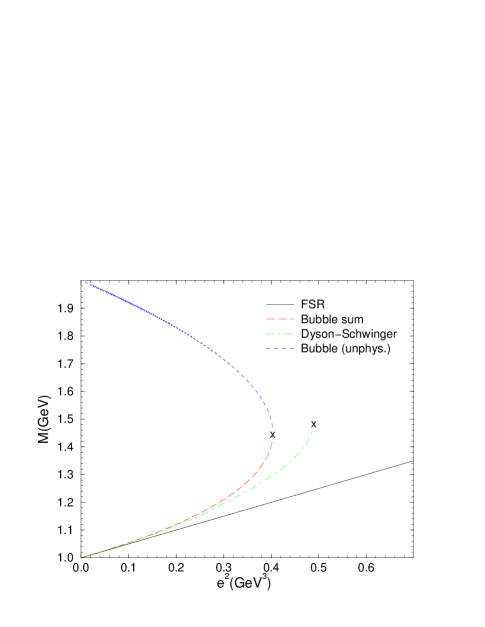
Figure 4: The function $M(e^{2})$, calculated in 0+1d with values of $m=\mu=1$ GeV, using the FSR approach, the Dyson-Schwinger equation in the rainbow approximation, and the bubble summation. While the exact result is always real, the rainbow DSE and the bubble summation results become complex beyond a critical coupling.

It is interesting to note that the simple bubble summation and the rainbow Dyson-Schwinger results display similar behavior. While the exact result provided by the FSR linearly increases for all coupling strengths, both the simple bubble summation and the rainbow Dyson-Schwinger results come to a critical point beyond which solutions for the dressed masses become complex. This example very clearly shows that conclusions about the mass poles of propagators based on approximate methods such as the rainbow Dyson-Schwinger equation can be misleading.

In general a consistent treatment of any nonperturbative calculation must involve summation of all possible vertex corrections. Vertex corrections are those irreducible diagrams that surround an interaction vertex. The elementary vertex is the three-point vertex, $\Gamma_{3}$, but the particle interactions will lead to the appearance of $n$th order irreducible vertices, $\Gamma_{n}$, as illustrated in Fig. 5.

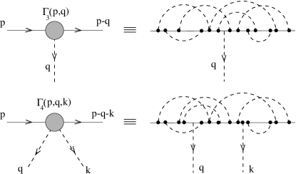
Figure 5: Because of the interactions, the one-particle irreducable vertex functions $\Gamma_{n}$ $(n=3,4,\cdots)$ depend on the external momenta.

The propagation of a bound state therefore involves a summation of all diagrams with the inclusion of higher order vertices (Fig. 6). A rigorous determination of all of these vertices is not feasible. In the literature on bound states $\Gamma_{n>3}$ interaction vertices are usually completely ignored. The 3-point vertex $\Gamma_{3}$ can be approximately calculated in the ladder approximation Maris (2000). However a rigorous determination of the exact form of the 3-point vertex is not possible, for this requires the knowledge of even higher order vertices.

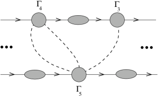
Figure 6: Exact computation of the two-body bound state propagator requires the summation of all particle self energies, vertex corrections, and ladder and crossed ladder exchanges.

In order to be able to make a connection between the exact theory and predictions based on approximate bound state equations it is essential that the role of interaction vertices be understood. The Feynman-Schwinger Representation (FSR) is a useful technique for this purpose.

We now present the interesting outcome, that the full bound state result dictated by a Lagrangian can be obtained by summing only generalized ladder diagrams (“generalized” ladders include both crossed ladders and, in theories with an elementary four-point interaction, both overlapping and non-overlapping “triangle” and “bubble” diagrams).

We adopt the following procedure for determining the contribution of vertex corrections in 3+1 dimension. We start with an initial bare mass $m$ and calculate the full two-body bound state result with the inclusion of all interactions: generalized ladders, self energies and vertex corrections. Let us denote the result for the exact two-body bound state mass by $M_{2}^{\rm tot}(e^{2},m)$, since it will be a function of the coupling strength $e$ and the bare input mass $m$, and the superscript “tot” implies that all interactions are summed. Next we calculate the dressed one-body mass $M_{1}(e^{2},m)$. Then using the dressed mass value $M_{1}(e^{2},m)$ we calculate the bound state mass $M_{2}^{\rm exch}(e^{2},M_{1})$ by summing only the generalized exchange interaction contributions. In this last calculation we sum only exchange interactions (generalized ladders), but the self energy is approximately taken into account since we use the (constant) dressed one-body mass as input. However the vertex corrections and wavefunction renormalization are completely left out since we use the original vertex provided by the Lagrangian. In order to compare the full result where all interactions have been summed with the result obtained by two dressed particles interacting only by generalized ladder exchanges we plot the bound state masses obtained by these methods. Numerical results are presented in Fig. 7. This result is qualitatively similar to that obtained analytically for SQED in 0+1 dimension Savkli, Gross, and Tjon (2002).

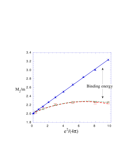
Figure 7: Two-body bound state mass for SQED in 3+1 dimensions. Solid triangles are 2$M_{1}$, open squares are $M_{2}^{\rm exch}$, and open triangles are $M_{2}^{\rm tot}$. Here $\mu/m=0.15$, $\Lambda_{1}/\mu=3$, and $\Lambda_{2}/\mu=5$. The smooth lines are fits to the “data”. Note that $M_{2}^{\rm exch}=M_{2}^{\rm tot}$ to within errors.

The numerical results presented here yield the following prescription for bound state calculations: In order to get the full result for bound states it is a good approximation to first solve for dressed one-body masses exactly (summing all generalized rainbow diagrams), and then use these dressed masses and the bare interaction vertex provided by the Lagrangian to calculate the bound state mass by summing only generalized ladder interactions (leaving out vertex corrections). In terms of Feynman graphs this prescription can be expressed as in Fig. 8

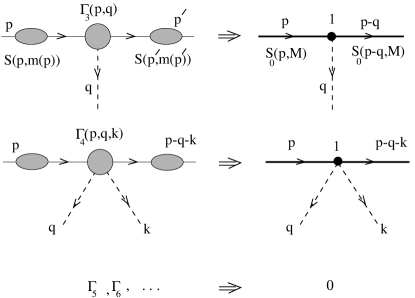
Figure 8: The correct two-body result can be obtained by simply using a dressed constituent mass and a bare vertex, and ignoring the contributions of higher order vertices.

The significance of the results presented above rests in the fact that the problem of calculating exact results for bound state masses in SQED has been reduced to that of calculating only generalized ladders. Summation of generalized ladders can be addressed within the context of bound state equations Gross (1969, 1982); Phillips, Wallace, and Devine (1998). Here we have shown the connection between the full prediction of a Lagrangian and the summation of generalized ladder diagrams. Our results are rigouous for SQED, but are only suggestive for more general theories with spin or internal symmetries. Since we have neglected charged particle loops (our results are in quenched approximation), and the current is conserved in SQED, it is perhaps not surprising that the bare coupling is not renormalized, but the fact that the momentum dependence of the dressed mass and vertex corrections seem to cancel is unexpected. If we were to unquench our calculation, or to use a theory without a conserved current, it is reasonable to expect that both the bare interaction and the mass would be renormalized.

Finally, we call attention to a remarkable cancellation that occurs in the one-body calculations. The exact self energy shown in Fig. 7 (and also in Fig. 4 for different parameters) is nearly linear in $e^{2}$ Savkli, Gross, and Tjon (2000). This remarkable fact implies that the exact self energy is well approximated by the lowest order result from perturbation theory. It is instructive to see how this comes about. If we expand the self energy to fourth order, expanding each term about the bare mass $m$, we have

$$S^{-1}_{d}(p^{2}) = m^{2}-p^{2}+\Sigma(p^{2})$$ (36)

$$= m^{2}-p^{2}+\Sigma_{2}+(p^{2}-m^{2})\Sigma_{2}^{\prime}$$

$$+\Sigma_{4}\,,\quad$$

where $\Sigma_{\ell}=\Sigma_{\ell}(m^{2})$ is the contribution of order $e^{\ell}$ evaluated at $p^{2}=m^{2}$, $\Sigma^{\prime}=d\Sigma(p^{2})/dp^{2}$ evaluated at $p^{2}=m^{2}$, and the formula is valid for $p^{2}-m^{2}\simeq e^{2}$. Expanding the dressed mass in a power series in $e^{2}$

$$M_{1}^{2} = m^{2}+m_{2}^{2}+m_{4}^{2}+\cdots\,,$$ (37)

where $m_{\ell}^{2}$ is the contribution of order $e^{\ell}$, and substituting into Eq. (36), give

$$M_{1}^{2} = m^{2}+\Sigma_{2}+\Sigma_{2}^{\prime}\Sigma_{2}+\Sigma_{4}+\cdots\,,$$ (38)

The mass is then

$$M_{1} = m+\frac{\Sigma_{2}}{2m}+\frac{4m^{2}\left[\Sigma_{2}^{\prime}\Sigma_{2}+\Sigma_{4}\right]-\Sigma_{2}^{2}}{8m^{3}}$$ (39)

$$+\cdots\,,\qquad$$

The linearity of the exact result implies that the forth order term in Eq. (39) must be zero (or very small), and this can be easily confirmed by direct calculations!

The cancellation of the fourth order mass correction (and all higher orders) is reminisent of the cancellations between generalized ladders that explains why quasipotential equations are more effective that the ladder Bethe-Salpeter equation in explaining 2-body binding energies. It shows that a simple evaluation of the second order self energy at the bare mass point is more accurate than solution of the Dyson Schwinger equation in rainbow approximation.

The general lesson seems to be that attempts to sum a small subclass of diagrams exactly is often less accurate than the approximate summation of a larger class of diagrams.

In the next section we consider the application of the FSR approach to scalar $\chi^{2}\phi$ interaction

IV Scalar $\chi^{2}\phi$ interaction with the FSR approach

We consider the theory of charged scalar particles $\chi$ of mass $m$ interacting through the exchange of a neutral scalar particle $\phi$ of mass $\mu$. The Euclidean Lagrangian for this theory is given by

$${\cal L} = \chi^{*}\bigl{[}m^{2}-\partial^{2}+g\phi\bigr{]}\chi+\frac{1}{2}\,\phi(\mu^{2}-\partial^{2})\phi.$$ (40)

The 2-body propagator for the transition from the initial state $\Phi_{i}=\chi^{*}(x)\chi(\bar{x})$ to final state $\Phi_{f}=\chi^{*}(y)\chi(\bar{y})$ is given by

$$G(y,\bar{y}|x,\bar{x})=N\bigg{\lmoustache}{\cal D}\chi^{*}\bigg{\lmoustache}{\cal D}\chi\bigg{\lmoustache}{\cal D}\phi\,\,\,\Phi^{*}_{f}\,\Phi_{i}\,\,{\rm exp}\biggl{[}-\int d^{4}x\,{\cal L}\biggr{]},$$ (41)

After the usual integration of matter fields is done, the Green’s function reduces to

$$G(y,\bar{y}|x,\bar{x}) = N\bigg{\lmoustache}{\cal D}\phi\,({\rm det}S)\,\,S(x,y)S(\bar{x},\bar{y})\,e^{-L_{0}[\phi]}\,,$$ (42)

with the free Lagrangian, $L_{0}$, and the interacting propagator, $S(x,y)$, defined by

$$L_{0}[\phi] \equiv \frac{1}{2}\int d^{4}z\;\phi(z)(\mu^{2}-\partial_{z}^{2})\phi(z)$$

$$S(x,y) \equiv \langle y\,|\,\frac{1}{m^{2}+H(\hat{z},\hat{p})}\,|\,x\rangle\,,$$ (43)

with the Hamiltonian

$$H(\hat{z},\hat{p}) \equiv \hat{p}^{2}-g\phi(\hat{z})\,.$$ (44)

As in the case of scalar QED we employ the quenched approximation: ${\rm det}S\rightarrow 1$.

We exponentiate the denominator by introducing an $s$ integration along the imaginary axis with an $\epsilon$ prescription

$$S(x,y) = \int_{0}^{i\infty}ds\,\,\,e^{-s(m^{2}+i\epsilon)}\,\langle y\,|\,{\rm exp}[-sH]\,|\,x\rangle\,.$$ (45)

This representation should be compared with the representation used earlier in SQED Eq. (19). Here the integration is done along the imaginary axis because $H$ is not positive definite.

Again, a quantum mechanical path integral representation can be constructed by recognizing that Lagrangian corresponding to the $H$ of Eq. (44) is given by

$$L(z,\dot{z})=\frac{\dot{z}^{2}}{4}+g\phi(z)\,.$$ (46)

The path integral representation for the interacting propagator is therefore

$$S(x,y) = -i\bigg{\lmoustache}_{0}^{\infty}ds\,\bigg{\lmoustache}\,{\cal D}z\,\,{\rm exp}\biggl{[}is(m^{2}+i\epsilon)-\frac{i}{4}\int_{0}^{s}d\tau\,\dot{z}^{2}(\tau)+ig\int_{0}^{s}d\tau\,\phi(z(\tau))\,\,\biggr{]}.$$ (47)

This representation allows the elimination of the integral over the exchange field $\phi$. The 2-body propagator reduces to

$$G = -\bigg{\lmoustache}_{0}^{\infty}ds\,\,\bigg{\lmoustache}_{0}^{\infty}d\bar{s}\,\,\bigg{\lmoustache}\,({\cal D}z)_{xy}\,\bigg{\lmoustache}\,({\cal D}\bar{z})_{\bar{x}\bar{y}}\,\,e^{iK[z,s]+iK[\bar{z},\bar{s}]}I_{\phi}\,,$$ (48)

where mass and kinetic term is given by

$$K[z,s] = (m^{2}+i\epsilon)s-\frac{1}{4s}\int_{0}^{1}d\tau\,\dot{z}^{2}(\tau)\,.$$ (49)

The field integration $I_{\phi}$ is a standard gaussian integration

$$I_{\phi} \equiv \biggl{\lmoustache}{\cal D}\phi\,{\rm exp}\biggl{[}+ig\biggl{(}\int_{0}^{s}d\tau\,\phi(z(\tau))+\int_{0}^{\bar{s}}d\bar{\tau}\,\phi(\bar{z}(\bar{\tau}))\biggr{)}-L_{0}[\phi]\biggr{]}$$ (50)

$$\equiv {\rm exp}\biggl{(}-V_{0}[z,s]-2\,V_{12}[z,\bar{z},s,\bar{s}]-V_{0}[\bar{z},\bar{s}]\biggr{)},$$

where $V_{0}$ and $V_{12}$ (self and exchange energy contributions in Fig. 9) are defined by

$$V_{0}[z,s] = \frac{g^{2}}{2}\,\,s^{2}\,\,\bigg{\lmoustache}_{0}^{1}d\tau\bigg{\lmoustache}_{0}^{1}d\tau^{\prime}\,\Delta(z(\tau)-z(\tau^{\prime}),\mu)\equiv s^{2}\,v[z]$$ (51)

$$V_{12}[z,\bar{z},s,\bar{s}] = \frac{g^{2}}{2}\,\,s\bar{s}\,\,\bigg{\lmoustache}_{0}^{1}d\tau\bigg{\lmoustache}_{0}^{1}d\bar{\tau}\,\Delta(z(\tau)-\bar{z}(\bar{\tau}),\mu)\,.$$ (52)

It should be noted that the interaction terms explicitly depend on the $s$ variable, which was not the case for SQED. The interaction kernel $\Delta$ is given by

$$\Delta(x,\mu) = \bigg{\lmoustache}\frac{d^{4}p}{(2\pi)^{4}}\frac{e^{ip\cdot x}}{p^{2}+\mu^{2}}$$ (53)

$$= \frac{\mu}{4\pi^{2}|x|}K_{1}(\mu|x|)\,.$$

In order to be able to compute the path integral over trajectories, a discretization of the path integral is needed

$$({\cal D}z)_{xy} \rightarrow (N/4\pi s)^{2N}\Pi^{N-1}_{i=1}\bigg{\lmoustache}d^{4}z_{i}\,.$$ (54)

The $s$ dependence is crucial for correct normalization. After discretization, the 1-body propagator takes the following form

$$G = i\left(\frac{N}{4\pi}\right)^{2N}\bigg{\lmoustache}\Pi_{i=1}^{N-1}dz_{i}\bigg{\lmoustache}_{0}^{\infty}\frac{ds}{s^{2N}}\,{\rm exp}\biggl{[}im^{2}s-i\frac{k^{2}}{4s}-s^{2}\,v[z]\biggr{]},$$ (55)

where $v[z]$ was defined in Eq. (51). This is an oscillatory and regular integral and it is not convenient for Monte-Carlo integration. The origin of the oscillation is the fact that $s$ integral was defined along the imaginary axis,

$${\rm Rep.\,\,1:}\,\,\,\,S(x,y)=<y\,|\bigg{\lmoustache}_{0}^{-i\infty}ds\,{\rm exp}\biggl{[}-s(m^{2}-\partial^{2}+g\phi+i\epsilon)\biggr{]}|\,x>\,.$$ (56)

In earlier works Simonov (1989); Nieuwenhuis, and Tjon (1996) a nonoscillatory Feynman-Schwinger representation was used,

$${\rm Rep.\,\,2:}\,\,\,\,S(x,y)=<y\,|\bigg{\lmoustache}_{0}^{\infty}ds\,{\rm exp}\biggl{[}-s(m^{2}-\partial^{2}+g\phi)\biggr{]}|\,x>\,.$$ (57)

Rep. 2 leads to a nonoscillatory and divergent result

$$G \propto \bigg{\lmoustache}_{0}^{\infty}\frac{ds}{s^{2N}}\,{\rm exp}\biggl{[}-m^{2}s-\frac{k^{2}}{4s}+s^{2}v[z]\biggr{]},$$ (58)

and the large $s$ divergence was regulated by a cut-off $\Lambda$. This is not a satisfactory prescription since it relies on an arbitrary cut-off. Later it was shown Savkli, Gross, and Tjon (1999); Savkli (2001) that the correct procedure is to start with Rep.1 and make a Wick rotation such that the final result is nonoscillatory and regular. The implementation of Wick rotation however is nontrivial. Consider the s-dependent part of the integral for the 1-body propagator

$$G \propto \bigg{\lmoustache}_{0}^{\infty}\frac{ds}{s^{2N}}\,{\rm exp}\biggl{[}im^{2}s-i\frac{k^{2}}{4s}-s^{2}\,v[z]\biggr{]},$$ (59)

It is clear that a replacement of $s\rightarrow is$ leads to a divergent result. The problem with the Wick rotation (Fig 10) comes from the fact that the $s$ integral is infinite both along the imaginary axis and along the contour at infinity. These two infinities cancel to yield a finite integral along the real axis.

Figure 9: Sample trajectories with self and exchange interactions.

Figure 10: Wick rotation in the $s$ integration.

As $g\rightarrow 0$ the dominant contribution to the $s$ integral in Eq. (59) comes from the stationary point

$$s=is_{0}\simeq i\frac{k}{2m}.$$ (60)

Therefore one might suppress the integrand away from the stationary point by introducing a damping factor $R$

$$R(s,s_{0}) \equiv 1-(s-is_{0})^{2}/\Gamma^{2}.$$ (61)

With this factor the integral in Eq. (59) is modified

$$G\propto\bigg{\lmoustache}_{0}^{\infty}\!\!\frac{ds}{s^{2N}}\,{\rm exp}\biggl{[}im^{2}s-i\frac{k^{2}}{4s}-\frac{s^{2}\,v[z]}{R^{2}(s,s_{0})}\biggr{]}\,.$$

(62)

This modification allows us to make a Wick rotation since the contribution of the contour at infinity now vanishes. However this procedure relies on the fact that there exists a stationary point. It can be seen from the original expression Eq. (59) that this is not always true. According to the original integral the stationary point is given by the following equation

$$im^{2}+i\frac{k^{2}}{4s^{2}}-2s\,v[z] = 0\,.$$ (63)

Introducing $s=i{\rm s}\frac{k}{2m}$ and ${\rm g}^{2}=k\left<v[z]\right>/m^{3}$ this equation becomes

$$-1+{\rm s}^{2}-{\rm g}^{2}{\rm s}^{3}=0\,.$$ (64)

The stationary point is determined by the first intersection of a cubic plot with the positive s axis as shown in Fig. 11. The plot in Fig. 11 shows that, as the effective coupling strength g² is increased the curve no longer crosses the positive s axis. Therefore beyond a critical coupling strength the stationary point vanishes and mass results should be unstable.

Figure 11: As the effective coupling strength g² is increased, the stationary point disappears.

Limiting discussion to cases where the original expression Eq. (59) has a critical point, we now turn to perform a Wick rotation on the modified expression Eq. (62). The Wick rotation in Eq. (62) amounts to a simple replacement $s\rightarrow is$, and a regular, nonoscillatory integral is found:

$$G\propto\bigg{\lmoustache}_{0}^{\infty}\frac{ds}{s^{2N}}\,{\rm exp}\biggl{[}-m^{2}s-\frac{k^{2}}{4s}+\frac{s^{2}\,v[z]}{R^{2}(is,s_{0})}\biggr{]}\,.$$

(65)

At first look it seems that the new integral always has a stationary point determined by the following equation

$$-m^{2}+\frac{k^{2}}{4s^{2}}+\frac{2s\,v[z]}{R^{2}(is,s_{0})}$$

$$\qquad-s^{2}v[z]\frac{(R^{2}(is,s_{0}))^{\prime}}{R^{2}(is,s_{0})}=0.$$ (66)

The key point to remember is that the stationary point we find after the Wick rotation should be the same stationary point we had before the Wick rotation. This is required to make sure that the physics remains the same after the Wick rotation. Self consistency therefore requires that the stationary point after the Wick rotation is at $s=is_{0}$. In that case $R(is_{0},s_{0})=1$, and $(R^{2}(is_{0},s_{0}))^{\prime}=0$ and Eq. (66) determining the critical point reduces to the earlier original Eq. (63).

The regularization of the ultraviolet singularities is done using Pauli-Villars regularization, which is particularly convenient for numerical integration since it only involves a change in the interaction kernel

$$\Delta(x,\mu) \longrightarrow \Delta(x,\mu)-\Delta(x,\alpha\mu).$$ (67)

Calculations of the $\chi^{2}\phi$ interaction in 3+1d require numerical Monte-Carlo integration. The first step is to represent the particle trajectories by a discrete number of $N+1$ points with

Figure 12: Number of steps a particle takes between initial and final coordinates is discretized. The space-time is continuous and there are no space-time boundaries

boundary conditions given by

$$z_{0}=x=(x_{1},x_{2},x_{3},0)$$

$$z_{N}=y=(y_{1},y_{2},y_{3},T)\,.$$ (68)

The discretization employed in the FSR is for the number of time steps a particle takes in going from the initial time to the final time along a trajectory in a 4-d coordinate space. This is very different from the discretization employed in lattice gauge theory. Contrary to lattice gauge theory, in the FSR approach space-time is continuous and rotational symmetry is respected. An additional, important benefit is the lack of space-time lattice boundaries, which allows calculations of arbitrarily large systems using the FSR approach. This feature provides an opportunity for doing complex applications such as calculation of the form factors of large systems.

In doing Monte-Carlo sampling we sample trajectories (lines) rather than gauge field configurations (in a volume). This leads to a significant reduction in the numerical cost. The ground state mass of the Green’s function is obtained using

$$m_{0}=\frac{\int{\cal D}Z\,S^{\prime}[Z]e^{-S[Z]}}{\int{\cal D}Z\,e^{-S[Z]}}.$$ (69)

Sampling of trajectories is done using the standard Metropolis algorithm, which insures that configurations sampled are distributed according to the weight $e^{-S[Z]}$. In sampling trajectories the final state (spacial) coordinates of particles can be integrated over, which puts the system at rest and projects out the $S$-wave ground state. As trajectories of particles are sampled, the wave function of the system can be determined simply by storing the final state configurations of particles in a histogram.

In sampling trajectories the first step is thermalization. In order to insure that the initial configuration of trajectories has no effect on results, the first 1000 or so updates are not taken into account. Statistical independence of subsequent samplings is measured by the correlation function $X(n)$, defined as

$$X(n) \equiv \frac{\left<m(i)m(i+n)\right>-\left<m\right>^{2}}{\left<m\right>^{2}},$$ (70)

where $m(i)$ is the mass measurement at the $i$’th update.

In order to insure that the location of the stationary point is self consistent, as discussed earlier, its location must be determined carefully. The stationary point can be parametrized by $s_{0}=CT/(2m)$, where $T/2m$ is the location of the stationary point when the coupling strength $g$ goes to zero. As the coupling strength is increased, the stationary point moves to larger values of $s_{0}$ (recall Fig. 11) and $C$ increases. Eventually a critical value of the coupling constant is reached beyond which there is no self consistent stationary point. In order to be able to do Monte-Carlo integrations, an initial guess must be made for the location of the stationary point. Self consistency is realized by insuring that the peak location of the s distribution in the Monte-Carlo integration agrees with the initial guess for the stationary point Savkli (2001). In Fig. 13 the dependence of the location of the stationary point on the coupling strength for 2-body bound states is shown. The figure shows that beyond the critical point $g^{2}\simeq 100$ GeV², $C$ goes to infinity implying that there is no stationary point. A similar critical behavior was also observed in Refs. Rosenfelder, and Schreiber (1996, 1996) within the context of a variational approach.

Figure 13: The dependence of the peak of s-distribution on the coupling strength for the 2-body bound state is shown. The peak location is given by $s_{0}=CT/2m$. There is no real solution for $C$ beyond $g^{2}=100$ GeV².

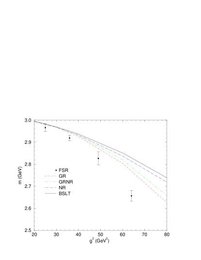
Figure 14: The coupling constant dependence of the 2-body bound state mass is shown. Beyond the critical coupling strength of $g^{2}=100$ GeV² the 2-body mass becomes unstable. The Bethe-Salpeter equation in the ladder approximation gives the smallest binding. The other models are described in the text.

In Fig. 14 FSR 2-body bound state mass results are shown for $m_{\chi}=1$ GeV, $\mu_{\phi}=0.15$ GeV. These results are all for a Pauli-Villars mass of 3$\mu$. Also are shown the predictions of various integral equation calculations.

The FSR calculation sums all ladder and crossed ladder diagrams, and excludes the self energy contributions. According to Fig. 14 all bound state equations underbind. Among the manifestly covariant equations the Gross equation (labeled GR in Fig. 14) gives the closest result to the exact calculation obtained by the FSR method. This is due to the fact that in the limit of infinitely heavy-light systems the Gross equation effectively sums all ladder and crossed ladder diagrams. The equal-time equation (labeled ET in Fig. 14) also produces a strong binding, but the inclusion of retardation effects pushes the ET results away from the exact results (Mandelzweig-Wallace equation Wallace, and Mandelzweig (1989), labeled MW in Fig. 14). In particular the Bethe-Salpeter equation in the ladder approximation (labeled BSE in Fig. 14) gives the lowest binding. Similarly the Blankenbecler-Sugar-Logunov-Tavkhelidze equation Logunov, and Tavkhelidze (1963); Blankenbecler, and Sugar (1963) (labeled BSLT in Fig. 14) gives a very low binding. A comparison of the ladder Bethe-Salpeter, Gross, and the FSR results shows that the exchange of crossed ladder diagrams plays a crucial role.

In Fig. 15 the dependence of the location of the stationary point on the coupling strength for 3-body bound states is shown.

Figure 15: The dependence of the peak of s-distribution on the coupling strength for the 3-body bound state mass is shown. The peak location is given by $s_{0}=CT/2m$. There is no real solution for $C$ beyond $g^{2}=81$ GeV².

In Fig. 16 the 3-body bound state results for 3 equal mass particles of mass 1 GeV are shown. For the 3-body case the only available results are for the Schrödinger and Gross equations. According to the results presented in Fig. 16, the bound state equations underbind for the 3-body case too. The Gross equation gives the closest result to the exact FSR result.

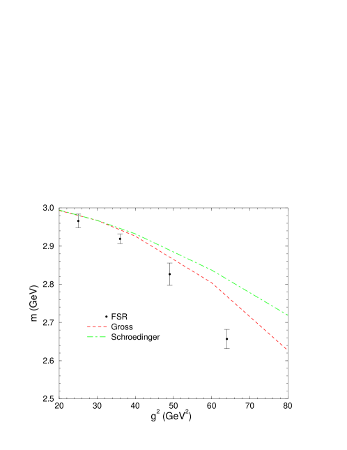
Figure 16: 3-body bound state results for 3 equal mass particles of mass 1 GeV.

Determination of the wavefunction of bound states is done by keeping the final state configurations of particles in a histogram. For example, for a 3-body bound state system, the probability distribution of the third particle for a given configuration of first and second particles is shown in Fig. 17. In the upper-left panel of Fig. 17, the two fixed particles are very close to each other so that the third particle sees them as a single particle. However as the fixed particles are separated from each other the third particle starts having a nonzero probability of being in between the two fixed particles (separation increases as we go from upper right to lower left panels in Fig. 17). Eventually when the two fixed particles are far away from each other the third particle has a nonzero probability distribution only at the origin (the lower left panel in Fig. 17).

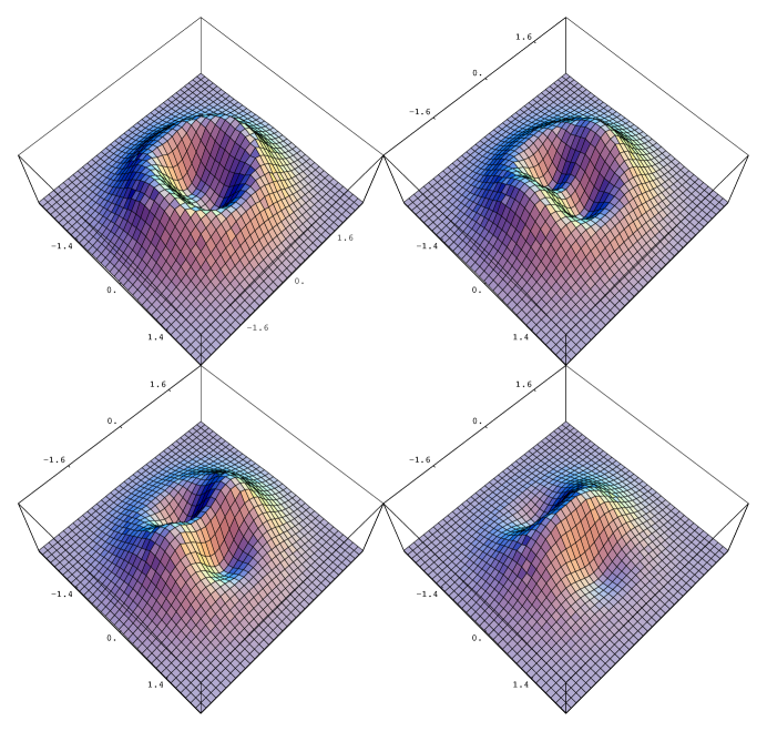
Figure 17: The four panels show the evolution of the probability distribution for the 3rd particle as the distance between the two fixed particles is increased. When the fixed particles are very close to each other the third particle sees them as a single particle (the upper left plot). As the fixed particles are separated, the third particle starts penetrating between them (2nd and 3rd panels), and when two fixed particles are far apart (as shown in the lower right panel), the third particle is most likely to be found between the two fixed particles.

Up to this point the FSR method has been derived and various applications to nonperturbative problems have been presented. In the next section we discuss the stability of the $\chi^{2}\phi$ theory.

V Stability of the scalar $\chi^{2}\phi$ interaction

Scalar field theories with a $\chi^{\dagger}\chi\phi$ interaction (which we will subsequently denote simply by $\chi^{2}\phi$) have been used frequently without any sign of instability, despite an argument in 1952 by DysonDyson (1952) suggesting instability, and a proof in 1959 by G. Baym Baym (1959) showing that the theory is unstable. For example, it is easy to show that, for a limited range of coupling values $0\leq g^{2}\leq g^{2}_{crit}$, the simple sum of bubble diagrams for the propagation of a single $\chi$ particle leads to a stable ground state, and it is shown in Ref. Savkli, and Gross (1999) that a similar result also holds for the exact result in “quenched” approximation. However, if the scalar $\chi^{2}\phi$ interaction is unstable, then this instability should be observed even when the coupling strength $g$ is vanishingly small $g^{2}\rightarrow 0^{+}$, as pointed out recently by Rosenfelder and SchreiberRosenfelder, and Schreiber (1996) (see also Ref. Ding, and Darewych (2000)). Both the simple bubble summation and the quenched calculations do not exhibit this behavior. Why do the simple bubble summation and the exact quenched calculations produce stable results for a finite range of coupling values?

A clue to the answer is already provided by the simplest semiclasical estimate of the ground state energy. In this approximation the gound state energy is obtained by minimizing

$$E_{0}=m^{2}\chi^{2}+\frac{1}{2}\mu^{2}\phi^{2}-g\phi\chi^{2}\,,$$ (71)

where $m$ is the bare mass of the matter particles, and $\mu$ the mass of the “exchanged” quanta, which we will refer to as the mesons. The minimum occurs at

$$E_{0}=m^{2}\chi^{2}-g^{2}\frac{\chi^{4}}{2\mu^{2}}\,.$$ (72)

This is identical to a $\chi^{4}$ theory with a coupling of the wrong sign, as discussed by Zinn-JustinZinn-Justin (1989). The ground state is therefore stable (i.e. greater than zero) provided

$$g^{2}<g^{2}_{\rm crit}=\frac{2m^{2}\mu^{2}}{\chi^{2}}\,.$$ (73)

This simple estimate suggests that the theory is stable over a limited range of couplings if the strength of the $\chi$ field is finite. We now develop this argument more precisely and show under what conditions it holds.

Before presenting new results, we lay the foundation using the variational principle. In the Heisenberg representation the fields are expanded in terms of creation and annihilation operators that depend on time

$$\chi(t,\bf{r}) = \int d\tilde{k}_{m}\left[a(k)\,e^{-ik\cdot x}+b^{{\dagger}}(k)\,e^{ik\cdot x}\right]$$

$$\phi(t,\bf{r}) = \int d\tilde{k}_{\mu}\left[c(k)\,e^{-ik\cdot x}+c^{{\dagger}}(k)\,e^{ik\cdot x}\right]\,,$$

where $x=\{t,{\bf r}\}$ and

$$d\tilde{k}_{m}\equiv\frac{d^{3}k}{(2\pi)^{3}\,2E_{m}(k)}$$ (75)

with $E_{m}(k)=\sqrt{m^{2}+k^{2}}$. The equal-time commutation relations are

$$\left[a(k),a^{\dagger}(k^{\prime})\right]=(2\pi)^{3}\,2E_{m}(k)\,\delta^{3}(k-k^{\prime})\,.$$ (76)

The Lagrangian for the $\chi^{2}\phi$ theory is

$${\cal L}=\chi^{\dagger}\left[\partial^{2}-m^{2}+g\phi\right]\chi+\frac{1}{2}\,\phi\left(\partial^{2}-\mu^{2}\right)\phi\,,$$ (77)

and the Hamiltonian $H$ is a normal ordered product of interacting (or dressed) fields $\phi_{d}$ and $\chi_{d}$

$$H[\phi_{d},\chi_{d},t\,]=\int d^{3}r\,:\Biggl{\{}\left(\frac{\partial\chi_{d}}{\partial t}\right)^{2}+({\bf\nabla}\chi_{d})^{2}+m^{2}\chi_{d}^{2}$$

$$+\frac{1}{2}\biggl{[}\left(\frac{\partial\phi_{d}}{\partial t}\right)^{2}+(\vec{\nabla}\phi_{d})^{2}+\mu^{2}\phi_{d}^{2}\biggr{]}-g\chi_{d}^{2}\phi_{d}\Biggr{\}}:\,.$$ (78)

This hamitonian conserves the difference between number of matter and the number of antimatter particles, which we denote by $n_{0}$. Eigenstates of the Hamiltonian will therefore be denoted by $\left|n_{0},\lambda\right>$, where $\lambda$ represents the other quantum numbers that define the state. Hence, allowing for the fact that the eigenvalue may depend on the time,

$$H[\phi_{d},\chi_{d},t\,]\left|n_{0},\lambda\right>=M_{n_{0},\lambda}(t)\left|n_{0},\lambda\right>\,.$$ (79)

In the absence of an exact solution of (79), we may estimate it from the equation

$$M_{n_{0},\lambda}(t)= \left<n_{0},\lambda\right|H[\phi_{d},\chi_{d},t\,]\left|n_{0},\lambda\right>$$

$$= \left<n_{0},\lambda\right|U^{-1}(t,0)H[\phi,\chi,0\,]U(t,0)\left|n_{0},\lambda\right>$$

$$\equiv \left<n_{0},\lambda,t\right|H[\phi,\chi,0\,]\left|n_{0},\lambda,t\right>\,,$$ (80)

where $U(t,0)$ is the time translation operator which carries the Hamiltonian from time $t=0$ to later time $t$. We have also chosen $t=0$ to be the time at which the interaction is turned on, $\phi_{d}(t)=U^{-1}(t,0)\phi(0)U(t,0)$, and the last step simplifies the discussion by permitting us to work with a Hamiltonian constructed from the free fields $\phi$ and $\chi$. [If the interaction were turned on at some other time $t_{0}$, we would obtain the same result by absorbing the additional phases $\exp(\pm iEt_{0})$ into the creation and annhilation operators.]

At $t=0$ the Hamiltonian in normal order reduces to

$$H[\phi,\chi,0\,] = \int d\tilde{k}_{m}\,E_{m}(k)\,{\cal N}_{0}(k,k)+\int d\tilde{p}_{\mu}\,E_{\mu}(p)\,c^{\dagger}(p)c(p)$$ (81)

$$-\frac{g}{2}\int\,\frac{d\tilde{k}_{m}\,d\tilde{k^{\prime}}_{m}}{\omega(k-k^{\prime})}{\cal N}_{1}(k,k^{\prime})\biggl{[}c^{\dagger}(k^{\prime}-k)+c(k-k^{\prime})\biggr{]},$$

where

$${\cal N}_{0}(k,k^{\prime})=\left\{a^{\dagger}(k)a(k^{\prime})+b^{\dagger}(k)b(k^{\prime})\right\},$$

$${\cal N}_{1}(k,k^{\prime})={\cal N}_{0}(k,k^{\prime})+\left\{a^{\dagger}(k)b^{\dagger}(-k^{\prime})+a(-k)b(k^{\prime})\right\}$$ (82)

and $\omega(k)=\sqrt{\mu^{2}+{\bf k}^{2}}$. To evaluate the matrix element (80) we express the the eigenstates as a sum of free particle states with $n_{0}$ matter particles, $n_{\rm pair}$ pairs of $\chi{\bar{\chi}}$ particles, and $\ell$ mesons:

$$\left|n_{0},\lambda,t\right>\equiv\left|n_{0},\alpha(t),\beta(t)\}\right>=\frac{1}{\gamma(t)}\,\sum_{n_{\rm pair}=0}^{\infty}\sum_{\ell=0}^{\infty}\alpha_{n_{\rm pair}}(t)\beta_{\ell}(t)\left|n_{0},n_{\rm pair},\ell\right>,$$ (83)

where $\gamma(t)$ is a normalization constant (defined below), the time dependence of the states is contained in the time dependence of the coefficients $\alpha(t)$ and $\beta(t)$, and

$$\left|n_{0},n_{\rm pair},\ell\right>\equiv\int\frac{\left|k_{1},\cdots,k_{n_{1}};q_{1},\cdots,q_{n_{2}};p_{1},\cdots,p_{\ell}\right>}{\sqrt{(n_{0}+n_{\rm pair})!\,n_{\rm pair}!\,\ell!}}$$ (84)

with $n_{1}=n_{0}+n_{\rm pair}$, $n_{2}=n_{\rm pair}$ and

$$\int=\int\,\prod_{i=1}^{n_{1}}\,d\tilde{k_{i}}\,f(k_{i})\;\prod_{j=1}^{n_{2}}\,d\tilde{q_{j}}\,f(q_{j})\;\prod_{l=1}^{\ell}\,d\tilde{p_{l}}\,g(p_{l}).$$ (85)

The particle masses in $d\tilde{k}$ and $d\tilde{p}$ have been suppressed; their values should be clear from the context. The normalization of the functions $f(p)$ and $g(p)$ is chosen to be

$$\int d\tilde{k}\,f^{2}(k)=\int d\tilde{p}\,g^{2}(p)\equiv 1$$ (86)

which leads to the normalization

$$\left<n^{\prime}_{0},n^{\prime}_{\rm pair},\ell^{\prime}\,|\,n_{0},n_{\rm pair},\ell\right>= \delta_{n^{\prime}_{0},n_{0}}\,\delta_{n^{\prime}_{\rm pair},n_{\rm pair}}\,\delta_{\ell^{\prime},\ell}$$

$$\left<n_{0},\lambda,t\,|\,n_{0},\lambda,t\right>= 1\,,$$ (87)

if $\gamma(t)=\alpha(t)\beta(t)$ with

$$\alpha^{2}(t)= \sum_{n_{\rm pair}=0}^{\infty}\alpha_{n_{\rm pair}}^{2}(t)=\alpha(t)\cdot\alpha(t)$$

$$\beta^{2}(t)= \sum_{\ell=0}^{\infty}\,\beta_{\ell}^{2}(t)=\beta(t)\cdot\beta(t)\,.$$ (88)

The expansion coefficients $\{\alpha_{n_{\rm pair}}(t)\}$ and $\{\beta_{\ell}(t)\}$ are vectors in infinite dimensional spaces.

In principle the scalar cubic interaction in four dimensions requires ultraviolet regularization. However the issue of regularization and the question of stabilty are qualitatively unrelated. For example, the cubic interaction is also unstable in dimensions lower than four, where there is no need for regularization. The ultraviolet regularization would have an effect on the behavior of functions $f(p)$, and $g(p)$, which are left unspecified in this discussion except for their normalization.

The matrix element (80) can now be evaluated. Assuming that $f(k)=f(-k)$ and $g(k)=g(-k)$, it becomes:

$$M_{n_{0},\lambda}(t)=\left\{n_{0}+2L(t)\right\}\tilde{m}+G(t)\,\tilde{\mu}-gV\left\{n_{0}+2L(t)+2L_{1}(t)\right\}\,\sqrt{G_{1}(t)}\,,$$ (89)

where the constants $\tilde{m}$, $\tilde{\mu}$, and $V$ are

$$\tilde{m} \equiv \int\,d\tilde{k}\,E_{m}(k)\,f^{2}(k)\,,\quad\tilde{\mu}\equiv\int\,d\tilde{p}\,E_{\mu}(p)\,g^{2}(p)$$

$$V \equiv \int\,\frac{d\tilde{k}_{m}\,d\tilde{k}^{\prime}_{m}\,f(k)f(k^{\prime})g(k-k^{\prime})}{\sqrt{m^{2}+({\bf k}-{\bf k}^{\prime})^{2}}}\,,$$ (90)

and the time dependent quantities are

$$L(t)= \sum_{n_{\rm pair}=0}^{\infty}\frac{n_{\rm pair}\,\alpha^{2}_{n_{\rm pair}}(t)}{\alpha^{2}(t)},\quad G(t)=\sum_{\ell=0}^{\infty}\frac{\ell\,\beta_{\ell}^{2}(t)}{\beta^{2}(t)}$$

$$L_{1}(t)= \sum_{n_{\rm pair}=1}^{\infty}\frac{\sqrt{n_{0}+n_{\rm pair}}\sqrt{n_{\rm pair}}\;\alpha_{n_{\rm pair}}(t)\,\alpha_{{n_{\rm pair}}-1}(t)}{\alpha^{2}(t)}$$

$$\sqrt{G_{1}(t)}= \sum_{\ell=1}^{\infty}\frac{\sqrt{\ell}\;\beta_{\ell}(t)\beta_{\ell-1}(t)}{\beta^{2}(t)}\,.$$ (91)

Note that $L$ and $G$ are the average number of matter pairs and mesons, respectively, in the intermediate state.

The variational principle tells us that the correct mass must be equal to or larger than (89). This inequality may be simplified by using the Schwarz inequality to place an upper limit on the quantities $L_{1}$ and $G_{1}$. Introducing the vectors

$$f_{1}= \{\alpha_{1},\sqrt{2}\,\alpha_{2},\cdots\}=\{\sqrt{n}\;\alpha_{n}\}$$

$$f_{2}= \{\sqrt{n_{0}+1}\,\alpha_{0},\sqrt{n_{0}+2}\,\alpha_{1},\cdots\}=\{\sqrt{n_{0}+n}\;\alpha_{n-1}\}$$

$$h= \{\beta_{1},\sqrt{2}\,\beta_{2},\cdots\}=\{\sqrt{\ell}\;\beta_{\ell}\}\,,$$ (92)

we may write

$$L_{1}(t)=\frac{f_{1}(t)\cdot f_{2}(t)}{\alpha^{2}(t)} \leq\frac{\sqrt{f_{1}^{2}(t)\,f_{2}^{2}(t)}}{\alpha^{2}(t)}$$

$$=\sqrt{L(t)\{n_{0}+1+L(t)\}}$$

$$\sqrt{G_{1}(t)}=\frac{h(t)\cdot\beta(t)}{\beta^{2}(t)} \leq\frac{\sqrt{h^{2}(t)\beta^{2}(t)}}{\beta^{2}(t)}=\sqrt{G(t)}\,.$$ (93)

Hence, suppressing explicit reference to the time dependence of $L$ and $G$, Eq. (89) can be written

$$M_{n_{0},\lambda}(t)\geq\left(n_{0}+2L\right)\tilde{m}+G\,\tilde{\mu}-gV\left\{\left(\sqrt{n_{0}+1+L}+\sqrt{L}\right)^{2}-1\right\}\,\sqrt{G}\,.$$ (94)

Minimization of the ground state energy with respect to the average number of mesons $G$ occurs at

$$\sqrt{G_{0}}=\frac{gV}{2\tilde{\mu}}\,\left\{\left(\sqrt{n_{0}+1+L}+\sqrt{L}\right)^{2}-1\right\}\,.$$ (95)

At this minimum point the ground state energy is bounded by

$$M_{n_{0},\lambda}(t)\geq \left\{n_{0}+2L\right\}\tilde{m}-\mu G_{0}\,.$$ (96)

If we continue with the minimization process we would obtain $M_{n_{0},\lambda}(t)\to-\infty$ as $L\to\infty$, providing no lower bound and hence suggesting that the state is unstable. However, if L is finite, this result shows that the ground state is stable for couplings in the interval $0<g^{2}<g_{crit}^{2}$ with

$$g_{crit}^{2}\equiv\frac{4\,\tilde{\mu}\,\tilde{m}\,(n_{0}+2L)}{V^{2}\left\{\left(\sqrt{n_{0}+1+L}+\sqrt{L}\right)^{2}-1\right\}^{2}}\,.$$ (97)

This interval is nonzero if the number of matter particles, $n_{0}$, and the average number of $\chi\bar{\chi}$ pairs, $L$, is finite. In particular, if there are no $Z$ diagrams or $\chi\bar{\chi}$ loops in the intermediate states, then the ground state will be stable for a limited range of values of the coupling.

This result also suggests strongly that the system is unstable when $g^{2}>g^{2}_{\rm crit}$, or when $L\to\infty$ (implying that $g^{2}_{\rm crit}\to 0$). However, since Eq. (96) is only a lower bound, our argument does not provide a proof of these latter assertions.

We now discuss the effect of the Z-graphs and of the matter loops on the stability. Using the Feynman-Schwinger representation (FSR), we will show that the ground state is (i) stable when $Z$-diagrams are included in intermediate states, but (ii) unstable when matter loops are included.

The covariant trajectory $z(\tau)$ of the particle is parametrized in the FSR as a function of the proper time $\tau$. In $\chi^{2}\phi$ theory the FSR expression for the 1-body propagator for a dressed $\chi$-particle in quenched approximation in Euclidean space was given qualitatively in Eq. (65). The detailed expression, needed in the following discussion, is

$$G(x,y) = \int_{0}^{\infty}ds\left[\frac{N}{4\pi s}\right]^{2N}\;\prod^{N-1}_{i=1}\int d^{4}z_{i}$$ (98)

$$\times\exp\biggl{\{}-K[z,s]-V[z,s_{r}]\biggr{\}}\,,\qquad$$

where the integrations are over all possible particle trajectories (discretized into $N$ segments with $N-1$ variables $z_{i}$ and boundary conditions $z_{0}=x$, and $z_{N}=y$) and the kinetic and self energy terms are

$$K[z,s] = m^{2}s+\frac{N}{4s}\sum_{i=1}^{N}(z_{i}-z_{i-1})^{2}\,,$$ (99)

$$V[z,s] = -\frac{g^{2}s^{2}}{2N^{2}}\sum_{i,j=1}^{N}\Delta\left(\delta z_{ij},\mu\right)\,,$$ (100)

where $\Delta(z,\mu)$ is the Euclidean progagator of the meson (suitably regularized), $\delta z_{ij}=\frac{1}{2}(z_{i}+z_{i-1}-z_{j}-z_{j-1})$, and

$$s_{r}\equiv\frac{s}{R(s,s_{0})}=\frac{s}{1+(s-s_{0})^{2}/\Gamma^{2}}\,.$$ (101)

(The need for the substitution $s\to s_{r}$ was discussed above in Sec. IV.)

In preparation for a discussion of the effects of $Z$-diagrams and loops, we first discuss the stability of Eq. (98) when neither $Z$-diagrams nor loops are present. To make the discussion explicit, consider the one body propagator in 0+1 dimension. Since the integrals converge, we make the crude approximation that each $z_{i}$ integral is approximated by one point (since we are excluding $Z$-diagrams, the points may lie along the classical trajectory). If the boundary conditions are $z_{0}=0$ and $z_{N}=T$ the points along the classical trajectory are $z_{i}=iT/N$, and

$$K[z,s]=m^{2}s+\frac{N}{4s}\sum_{i=1}^{N}(z_{i}-z_{i-1})^{2}=m^{2}s+\frac{T^{2}}{4s}\,.$$ (102)

If the interaction is zero, this has a stationary point at $s=s_{0}=T/(2m)$, giving

$$K[z,s]=K_{0}=mT\,,$$ (103)

yielding the expected free particle mass $m$. [Note that half of this result comes from the sum over $(z_{i}-z_{i-1})^{2}$.] The potential term (100) may be similarily evaluated; it gives a negative contribution that reduces the mass.

We now turn to a discussion of the effect of $Z$-diagrams. For the simple estimate of the kinetic energy, Eq. (102), we chose integration points $z_{i}=iT/N$ uniformly spaced along a line. The classical trajectory connects these points without doubling back, so that they increase monotonically with proper time, $\tau$. However, since the integration over each $z_{i}$ is independent, there also exist trajectories where $z_{i}$ does not increase monotonically with $\tau$. In fact, for every choice of integration points $z_{i}$ there exist trajectories with $z_{i}$ monotonic in $\tau$ and trajectories with $z_{i}$ non-monotonic in $\tau$. The latter double back in time, and describe $Z$-diagrams in the path integral formalism. Two such trajectories that pass through the same points $z_{i}$ are shown in Fig. 18. These two trajectories contain the same points, $z_{i}$, but ordered in different ways, and both occur in the path integral.

Figure 18: It is possible to create particle-antiparticle pairs using folded trajectories. However folded trajectories are suppressed by the kinematics, as discussed in the text.

Now, since the total self energy is the sum of potential contributions $V[z,s]$ from all $(z_{i},z_{j})$ pairs, irrespective of how these coordinates are ordered, it must be the same for the straight trajectory $z(\tau)$ and the folded trajectory $z_{f}(\tau)$:

$$V[z_{f},s]=V[z,s]\,.$$ (104)

However, according to Eq. (99), the kinetic energy of the folded trajectory is larger than the kinetic energy of the straight trajectory

$$K[z_{f},s]>K[z,s]\,,$$ (105)

because it includes some terms with larger values of $(z_{i}-z_{i-1})^{2}$. Since the kinetic energy term is always positive, the folded trajectory ($Z$-graph) is always suppressed (has a larger exponent) compared with a corresponding unfolded trajectory (provided, of course, that $g^{2}<g^{2}_{\rm crit}$).

This argument holds only for cases where the trajectory does not double back to times before $z_{0}=0$ or after $z_{N}=T$. An example of such a trajectory is shown in Fig. 19 (upper panel). Here we compare this folded trajectory to another folded trajectory, $z^{\prime}_{f}$, with point $z_{1}$ closer to the starting point $z_{0}$ (lower panel of Fig. 19). This new folded trajectory has points spaced closer together, so that the kinetic energy is smaller and the potential energy is larger, and therefore

$$K[z_{f},s]-V[z_{f},s]>K[z^{\prime}_{f},s]-V[z^{\prime}_{f},s]\,.$$ (106)

It is clear that the larger the folding in the trajectory, the less energetically favorable is the path, and the most favorable path is again an unfolded trajectory with no points outside of the limits $z_{0}<z_{i}<z_{N}$.

While these arguments have been stated in 0+1 dimensions for simplicity, they are not dependent on the number of dimensions, and can be extended to the realistic case of 1+3 dimensions.

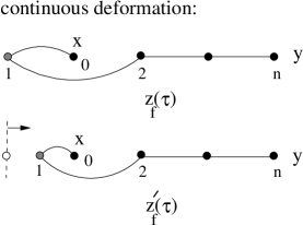
Figure 19: A folded trajectory at the end point of the path, and a similar one with $z_{1}$ closer to $z_{0}$.

We conclude that a calculation in quenched approximation, where the creation of particle-antiparticle pairs can only come from $Z$-graphs, must be more stable (produce a larger mass) than a similar calculation without any $\chi\bar{\chi}$ pairs. The quenched $\chi^{2}\phi$ theory therefore is bounded by the same limits given in Eq. (97). This conclusion supports, and is supported by, the results of Refs. Savkli, and Gross (1999); Savkli (2001, 2001) which show, in the quenched approximation, that the $\chi^{2}\phi$ interaction is stable for a finite range of coupling strengths.

It is now clear that the instability of $\chi^{2}\phi$ theory must be due to either (i) the possibility of creating an infinite number of closed $\chi\bar{\chi}$ loops, or (ii) the presence of an infinite number of matter particles (as in an infinite medium). Indeed, the original proof given by Baym used the possibility of loop creation from the vacuum to prove that the vacuum was unstable.

These results provide justification for the stability of relativistic one boson exchange models that usually exclude matter loops but may include $Z$-diagrams of all orders. Our argument cannot be easily extended to symmetric $\phi^{3}$ theories where it is impossible to make a clear distinction between $Z$-diagrams and loops.

VI Conclusions

In this paper we have given a summary results for scalar interactions obtained with the use of the FSR representation . The FSR approach uses a covariant path integral representation for the trajectories of particles. Reduction of field theoretical path integrals to path integrals involving particle trajectories reduces the dimensionality of the problem and the associated computational cost.

Applications of the FSR approach to 1 and 2-body problems in particular shows that uncontrolled approximations in field theory may lead to significant deviations from the correct result. Our results indicate that use of the Bethe-Salpeter equation in ladder approximation to solve the 2-body bound state problem is a poor approximation. For the scalar theories examined here, a better approximation to the 2-body problem is obtained using the Gross equation in ladder approximation. Similarly, use of the rainbow approximation for the 1-body problem gives a poorer result that simply calculating the self energy to second order! In all of these cases, the explanation for these results seems to be that the crossed diagrams (such as crossed ladders) play an essential role, canceling contributions from higher order ladder or rainbow diagrams.