Dynamical coupled-channel model of kaon-hyperon interactions

Abstract

The $\pi N\rightarrow KY$ and $KY\rightarrow KY$ reactions are studied using a dynamical coupled-channel model of meson-baryon interactions at energies where the baryon resonances are strongly excited. The channels included are: $\pi N$, $K\Lambda$, and $K\Sigma$. The resonances considered are: $N^{*}$ [$S_{11}(1650)$, $P_{11}(1710)$, $P_{13}(1720)$, $D_{13}(1700)$]; $\Delta^{*}$ [$S_{31}(1900)$, $P_{31}(1910)$, $P_{33}(1920)$]; $\Lambda^{*}$ [$S_{01}(1670)$, $P_{01}(1810)$] $\Sigma^{*}$ [$P_{11}(1660)$, $D_{13}(1670)$]; and $K^{*}$(892). The basic non-resonant $\pi N\rightarrow KY$ and $KY\rightarrow KY$ transition potentials are derived from effective Lagrangians using a unitary transformation method. The dynamical coupled-channel equations are simplified by parametrizing the $\pi N\rightarrow\pi N$ amplitudes in terms of empirical $\pi N$ partial-wave amplitudes and a phenomenological off-shell function. Two models have been constructed. Model A is built by fixing all coupling constants and resonance parameters using SU(3) symmetry, the Particle Data Group values, and results from a constituent quark model. Model B is obtained by allowing most of the parameters to vary around the values of model A in fitting the data. Good fits to the available data for $\pi^{-}p\to K^{\circ}\Lambda,~{}K^{\circ}\Sigma^{\circ}$ have been achieved. The investigated kinematics region in the center-of-mass frame goes from threshold to 2.5 GeV. The constructed models can be imbedded into associated dynamical coupled-channel studies of kaon photo- and electro-production reactions.

I Introduction

Investigation of kaon-nucleon and nucleon-hyperon interactions with hadronic probes has a long history in strangeness physics. However, the interactions involving an additional relevant kaon-hyperon channel have received marginal attention, because of lack of data. More recently, strangeness reactions are also receiving considerable attention in associated strangeness production with incident photon and electron beams. With the advent of facilities such as JLab, ELSA, Spring-8, and GRAAL, copious and high precision data on meson electromagnetic production on both nucleon and nuclear targets are becoming available. Measurements of the strangeness associated production channels focus on the energy region of $E_{\gamma}^{lab}\leq$ 2.5 GeV, corresponding to the total center-of-mass energy W$\leq$2.3 GeV, which cover the baryon resonances region. A result of our earlier work Chi01 on the $\gamma p\to K^{+}\Lambda$ reaction showed that multi-step processes, due to the coupling with the $\pi N$ channel, can have as much as a $20\%$ effect on the total cross-section. To investigate very recent strangeness production data, it is necessary to extend that work, which was limited to the $K\Lambda$ channel, to include all of the $K\Sigma$ channels: $\gamma p\to KY$, with $K\equiv K^{+},~{}K^{\circ}$ and $Y\equiv\Lambda,~{}\Sigma^{\circ},~{}\Sigma^{+}$. Accordingly, a dynamical coupled-channel investigation of these processes requires realistic models to describe $\pi N\to\pi N,~{}KY$, and $KY\to KY$ processes. The purpose of this paper is to report on our progress in this direction.

The importance of developing coupled-channel approaches to meson-baryon reactions is summarized as follows:

• Such an approach is required for a proper extraction of fundamental resonance decay properties, which are ultimately to be predicted by basic quark dynamics. In short, information about baryon resonance properties can only be reliably extracted within the context of an appropriate reaction theory. The importance of this interplay between extraction of fundamental information and the need for a consistent reaction theory has been emphasized by Sato and Lee Sat96 in the pion sector. Here we extend their investigation to the kaon sector.

• Impressive amounts of high quality data from JLab JLab , ELSA ELSA , LEPS LEPS , and GRAAL Graal offer us the opportunity to pin down the underlying reaction mechanism and to study the role and/or properties of intervening baryon resonances. Such an effort is a prerequisite for any attempt to search for missing resonances MissR . Combining models from a chiral constituent quark formalism Sagxx ; Sagxy with a coupled-channel approach, as presented in this work, is expected to provide reliable insights into the elementary strangeness photo- and electro-production reactions.

In recent years, coupled-channel effects on meson-baryon reactions with strangeness production have been investigated using two approaches. Kaiser et al. Kai97 applied a coupled-channel approach with chiral SU(3) dynamics to investigate pion- and photon-induced meson production near the $KY$ threshold. Although their recent results Car00 include p-wave multipoles, and thus reproduce data slightly above the threshold region, their chiral SU(3) dynamics model can not provide the higher partial waves that are important in describing the data at higher energies. Similar approaches have also been taken in Refs. Kri98 ; Oll00 ; Lut02 ; Hyo03 . Given the relevant W range mentioned above, their simplified dynamics represents of course only a first step. Indeed, comparisons with the $\pi N\to KY$ data clearly show that SU(3) models of Refs. Kai97 ; Hyo03 , even when p-waves interactions are included Car00 , greatly miss fitting the differential cross-sections: theoretical predictions produce slopes opposite to that required by the data.

The second coupled-channel approach used in the literature to investigate photon- and meson-induced reactions is based on using effective Lagrangians along with a K-matrix method, developed by the Giessen Group Feu98 ; Wal00 ; PM1 ; PM2 . In the $K$-matrix approach, all intermediate states are put on-energy-shell and hence possibly important off-shell dynamical effects are not accounted for. The advantage of this K-matrix approach is its numerical simplicity in handling a large number of coupled channels. However, the extracted $N^{*}$ parameters may suffer from interpretation difficulties in terms of existing hadron models, as explicitly demonstrated in an investigation Sat96 of the $\Delta$ resonance.

In this paper, we present a dynamical coupled-channel model in which the meson-baryon off-shell interactions are defined in terms of effective Lagrangians. This off-shell approach is achieved by directly extending existing dynamical models Sat96 for $\pi N$ scattering and pion photoproduction, to include $KY$ channels. The main feature of our approach is that the strong interaction matrix elements of $\pi N\rightarrow KY$ and $KY\rightarrow KY$ transition operators are derived from effective Lagrangians using the unitary transformation method of Ref. Sat96 . This derivation marks our major differences with chiral SU(3) coupled-channel models mentioned above Kai97 ; Car00 ; Kri98 ; Oll00 ; Lut02 ; Hyo03 since it allows one to include all relevant higher partial waves and our approach is also applicable at energies way above threshold. The dynamical content of our approach is also clearly very different from the on-shell $K$-matrix coupled-channel models Feu98 ; Wal00 ; PM1 ; PM2 .

It is necessary to indicate more precisely, and within a more general theoretical framework, the differences between our and other approaches . Similar to the well-studied meson-exchange models of $NN$ and $\pi N$ scattering, we also start with relativistic quantum field theory. With a model Lagrangian, there are two approaches for deriving models of meson-baryon scattering. The most common approach Kle74 is to find an appropriate three-dimensional reduction of the ladder Bethe-Salpeter equation of the considered model Lagrangian. Meson-baryon interactions are then identified with the driving terms of the resulting three-dimensional scattering equation; such as the Blankenbecler-Sugar bs or Gross gross equations. A fairly extensive study of the three-dimensional reductions for $\pi N$ scattering is given by Hung et al. Hung . Extending such reduction methods to derive coupled-channel equations with $stable$ two-particle channels is straightforward. In fact, the K-matrix coupled-channel equations employed in Refs. Feu98 ; Wal00 can be derived along this line if one further neglects that the principal-value parts of the meson-baryon propagators, which account for the off-shell dynamics. The scattering equations used in SU(3) chiral models of Refs. Kai97 ; Car00 ; Kri98 ; Oll00 ; Hyo03 can also be derived from the ladder Bethe-Salpeter equation using a procedure similar to a three-dimensional reduction, although this simplification is not spelled out explicitly by the authors. In Ref. Lut02 , the Bethe-Salpeter equation is solved directly, but only for the simplified case that the interaction kernel is of separable form due to the use of contact interactions. The difficulties in solving the Bethe-Salpeter equation, even with the ladder approximation, are well documented Keister .

Alternatively, one can construct models of meson-baryon interactions by deriving an effective Hamiltonian $H_{eff}$ defined in a chosen channel-space from a specific model Lagrangian. The scattering equation within the considered channel-space is then governed by standard scattering theory

$$S_{\alpha\beta}(E) = \delta_{\alpha,\beta}-2\pi iT_{\alpha\beta}(E),$$ (1)

$$T_{\alpha\beta}(E) = <\alpha\mid H_{I}+H_{I}\frac{1}{E-H_{0}-H_{I}+i\epsilon}H_{I}\mid\beta>,$$ (2)

where $\alpha,\beta$ represent the relevant channels, $S$ is the S-matrix and $T$ is the scattering operator. Here we have defined $H_{eff}=H_{0}+H_{I}$, with $H_{0}$ denoting the free Hamiltonian and $H_{I}$ defining the interactions between considered channels. This approach for $\pi N$ scattering and pion photo- and electro-production reactions has been pursued by Sato and Lee Sat96 . They applied the unitary transformation method of Refs. Sat91 ; SKO to derive $H_{eff}$ in a $\Delta\oplus\pi N\oplus\gamma N$ channel-space. The essential idea of the unitary transformation method we adopt is to eliminate unphysical vertex interactions $MB\to B^{\prime}$ with $m_{M}+m_{B}<m_{B^{\prime}}$ from the original field theory Hamiltonian (which can be constructed from a starting model Lagrangian using the standard canonical quantization procedure) and absorb their effects into $MB\to M^{\prime}B^{\prime}$ two-body interactions of the resulting $H_{eff}$. For the $\pi N$ scattering in the $\Delta$ region, the resulting effective Hamiltonian of the Sato-Lee model is

$$H_{eff}=H_{0}+v_{\pi N,\pi N}+\Gamma_{\Delta\leftrightarrow\pi N},$$ (3)

where $v_{\pi N,\pi N}$ is the non-resonant interaction and the $\Delta$ excitation is described by the vertex interaction $\Gamma_{\pi N\leftrightarrow\Delta}$. With the Hamiltonian Eq.(3), it is straightforward (as explained in Ref. Sat96 ) to show that the solution of Eq.(2) can be cast into the following form:

$$T_{\pi N,\pi N}(E)=t_{\pi N,\pi N}(E)+t^{R}_{\pi N,\pi N}(E),$$ (4)

where the non-resonant scattering operator $t_{\pi N,\pi N}$ is defined by the non-resonant potential $v_{\pi N,\pi N}$,

$$t_{\pi N,\pi N}(E)=v_{\pi N,\pi N}+v_{\pi N,\pi N}G_{\pi N}(E)t_{\pi N,\pi N}(E),$$ (5)

where the $\pi N$ propagator is defined by

$$G_{\pi N}(E)=\frac{1}{E-E_{\pi}({\bf k})-E_{N}({\bf p})+i\epsilon}\ ,$$ (6)

with $E_{\alpha}({\bf p})=\sqrt{{\bf p}^{2}+m_{\alpha}^{2}}$. The resonant amplitudes (in the center-of-mass frame) is

$$t^{R}_{\pi N,\pi N}(E)=\frac{\bar{\Gamma}^{\dagger}_{\Delta,\pi N}(E)\bar{\Gamma}_{\Delta,\pi N}(E)}{E-m^{0}_{\Delta}-\Sigma_{\Delta}(E)}\ ,$$ (7)

with

$$\bar{\Gamma}_{\Delta,\pi N}(E) = \Gamma_{\Delta\rightarrow\pi N}+\Gamma_{\Delta\rightarrow\pi N}G_{\pi N}(E)t_{\pi N,\pi N}(E),$$ (8)

$$\Sigma_{\Delta}(E) = \bar{\Gamma}_{\pi N}(E)G_{\pi N}(E)\Gamma_{\pi N\rightarrow\Delta}\ .$$ (9)

It is clear from the above equations that the resonant operator $t^{R}$ contains off-shell effects due to the non-resonant interaction $v_{\pi N,\pi N}$. Such off-shell effects must be accounted for in order to determine from the data the $bare$ vertex $\Gamma_{\Delta\leftrightarrow\pi N}$.

Figure 1: Graphical representation for $\sigma$-exchange $\pi N$ interaction.

For our later discussions, we now point out that the matrix elements of the effective Hamiltonian, Eq.(3), can be calculated from the usual Feynman diagrams once one specifies the time components of the propagators of intermediate states. For example, the $\sigma-$exchange (Fig. 1) of $v_{\pi N,\pi N}$ derived from the Lagrangian $L=g_{\sigma NN}\bar{\psi}_{N}(x)\psi_{N}(x)\phi_{\sigma}(x)+g_{\sigma\pi\pi}\phi_{\pi}(x)\phi_{\pi}(x)\phi_{\sigma}(x)$ is of the following form (with the normalization defined by Eqs. (1)-(2))

$$<{\bf p^{\prime}}{\bf k^{\prime}}\mid v^{(\sigma)}_{\pi N,\pi N}\mid{\bf p}{\bf k}> = \frac{g_{\sigma NN}g_{\sigma\pi\pi}}{(2\pi)^{3}}\frac{1}{\sqrt{2E_{\pi}(k^{\prime})}}\sqrt{\frac{m_{N}}{E_{N}(p^{\prime})}}I_{\sigma}\frac{1}{\sqrt{2E_{\pi}(k)}}\sqrt{\frac{m_{N}}{E_{N}(p)}},$$ (10)

with the propagator defined by

$$I_{\sigma}=\frac{1}{2}\left[\frac{1}{(E_{\pi}(k^{\prime})-E_{\pi}(k))^{2}-{\bf q}^{2}+m_{\sigma}^{2}+i\epsilon}+\frac{1}{(E_{N}(p^{\prime})-E_{N}(p))^{2}-{\bf q}^{2}-m_{\sigma}^{2}+i\epsilon}\right],$$ (11)

where ${\bf q}={\bf k}-{\bf k}^{\prime}={\bf p^{\prime}}-{\bf p}$ is the three-momentum transfer. In this Hamiltonian formulation, all particles are on their mass-shell, but the energies are not conserved during the collisions and hence $E_{\pi}(k^{\prime})-E_{\pi}(k)\neq E_{N}(p^{\prime})-E_{N}(p)$ in general. The $\sigma$ propagator form, given in Eq. (11), is not an arbitrary choice, but is rigorously defined by the selected unitary transformation. It is important to note that the matrix element, Eq. (10), is independent of the collision energy $E$ of Eqs. (1)-(2). If other methods, such as the Tamm-Dancoff method, are chosen, the resulting effective Hamiltonian could be energy-dependent, which then leads to non-trivial gauge invariant problems in applying the model to study meson photo- and electro-production reactions. The energy independence of the resulting $H_{eff}$ is an important feature of the unitary transformation method developed in Refs. Sat96 ; Sat91 . In this work we extend Eqs. (3)-(9) to include $KY$ channel and higher mass nucleon and hyperon resonances. The starting Lagrangians will be given later. The resulting effective $v_{\pi N,KY}$ and $v_{KY,KY}$ can be calculated from Feynman amplitudes with the rules illustrated in Eqs. (10)-(11).

Our goal is to construct models for describing all available data of differential cross-sections and polarization observables of the $\pi N\to KY$ reactions in the total center-of-mass energy range of W$\approx$1.3 to 2.3 GeV. These data Kna75 ; Bak78L ; Bak78S ; Sax80 ; Har80 ; Datax have been obtained a few decades ago with low intensity beams and therefore are not very extensive and not of high quality. Nevertheless, we will show that they give sufficient constraints on constructing models of $KY$ interactions.

In section II, we present the dynamical coupled-channel equations and explain our strategy in solving these equations. The results are given in section III. Section IV is devoted to Summary and Conclusions.

II Dynamical Coupled-Channel Equations

In this work, we consider a coupled-channel formulation obtained by extending Eqs. (3)-(9) to include the $KY$ channels. Specifically, we are interested in solving

$$T_{\alpha,\beta}(E)=t_{\alpha,\beta}(E)+t^{R}_{\alpha,\beta}(E),$$ (12)

where $\alpha,\beta\equiv\pi N,KY$. The non-resonant scattering operator is defined by

$$t_{\alpha,\beta}(E)=v_{\alpha,\beta}+\sum_{\delta=\pi N,KY}v_{\alpha,\delta}G_{\delta}(E)t_{\delta,\beta}(E),$$ (13)

where the propagators are defined by

$$G_{\pi N}(E) = \frac{1}{E-E_{\pi}({\bf k})-E_{N}({\bf p})+i\epsilon},$$ (14)

$$G_{KY}(E) = \frac{1}{E-E_{K}({\bf k})-E_{Y}({\bf p})+i\epsilon},$$ (15)

with $E_{\alpha}({\bf p})=\sqrt{{\bf p}^{2}+m_{\alpha}^{2}}$. The resonant amplitude (in the center-of-mass frame) is

$$t^{R}_{\alpha,\beta}(E)=\sum_{N^{*}_{i}}\frac{\bar{\Gamma}^{\dagger}_{N^{*}_{i},\alpha}(E)\bar{\Gamma}_{N^{*}_{i},\beta}(E)}{E-m^{0}_{N^{*}_{i}}-\Sigma_{N^{*}_{i}}(E)},$$ (16)

with

$$\bar{\Gamma}_{N^{*}_{i},\alpha}(E) = \Gamma_{N^{*}_{i}\rightarrow\alpha}+\sum_{\delta=\pi N,KY}\Gamma_{N^{*}_{i}\rightarrow\delta}G_{\delta}(E)t_{\delta,\alpha}(E),$$ (17)

$$\Sigma_{N^{*}_{i}}(E) = \sum_{\delta=\pi N,KY}\bar{\Gamma}_{N^{*}_{i}\rightarrow\delta}(E)G_{\delta}(E)\Gamma_{\delta\rightarrow N^{*}_{i}}.$$ (18)

In momentum-space, the matrix element of Eq. (13) in the center-of-mass frame is

$$t_{\beta\alpha}(\mathbf{p}^{\prime},\mathbf{p},E) = v_{\beta\alpha}(\mathbf{p}^{\prime},\mathbf{p})$$ (19)

$$+\sum_{\delta}\int d{\bf p}^{\prime\prime}v_{\beta\delta}({\bf p},{\bf p}^{\prime\prime})\frac{1}{E-E_{M_{\delta}}({\bf p}^{\prime\prime})-E_{B_{\delta}}({\bf p}^{\prime\prime})+i\epsilon}t_{\delta\alpha}(\mathbf{p}^{\prime\prime},\mathbf{p},E),$$

and the matrix element of the dressed vertex interaction Eq. (17) is

$$\bar{\Gamma}_{N^{*}_{i},\alpha}({\bf p},E) = \Gamma_{N^{*}\rightarrow\alpha}({\bf p})$$ (20)

$$+\sum_{\delta}\int d{\bf p}^{\prime}\Gamma_{N^{*}_{i}\rightarrow\delta}({\bf p}^{\prime})\frac{1}{E-E_{M_{\delta}}({\bf p}^{\prime})-E_{B_{\delta}}({\bf p}^{\prime})+i\epsilon}t_{\delta,\alpha}({\bf p}^{\prime},{\bf p},E).$$

The integrals in the above equations extend over the relative momentum ${\bf p}$, the off-shell dynamics is hence included in determining the scattering amplitudes. The K-matrix coupled-channel equation limit used by others can be obtained from the above equations only if one keeps the on-shell part (-$i\pi\delta(E-E_{M_{\delta}}({\bf p}^{\prime\prime})-E_{B_{\delta}}({\bf p}^{\prime\prime}))$ of the propagators.

II.1 Non-resonant amplitudes

Our first task is to define the nonresonant potentials for solving the coupled-channel equation (19). In the $K\Lambda$ threshold energy region, it is reasonable to derive the potentials involving the $KY$ channel using effective Lagrangians with SU(3) symmetry. On the other hand, it is not clear how to derive $\pi N$ potential $v_{\pi N,\pi N}$ for energies well above the $\pi N$ threshold region. We thus circumvent deriving $v_{\pi N,\pi N}$ and instead use a phenomenological procedure to include its effect using empirical $\pi N$ amplitudes Arn03 . Accordingly, the main outcome from our calculations are scattering operators for $\pi N\to KY$ and $KY\to KY$ transitions, which are also needed for dynamical coupled-channel studies of $\gamma N\to KY$ reactions.

To proceed, we first derive from Eq. (13) the following equations:

$$t_{KY,KY}(E) = V_{KY,KY}(E)+V_{KY,KY}(E)G_{KY}(E)t_{KY,KY}(E),$$ (21)

$$t_{KY,\pi N} = v_{KY,\pi N}+t_{KY,KY}(E)G_{KY}(E)v_{KY,\pi N},$$ (22)

where the effective $KY$ potential $V_{KY,KY}(E)$ is defined by

$$V_{KY,KY}(E)=v_{KY,KY}+v_{KY,\pi N}[G_{\pi N}(E)+G_{\pi N}(E)t_{\pi N,\pi N}(E)G_{\pi N}(E)]v_{\pi N,KY},$$ (23)

with

$$t_{\pi N,\pi N}(E)=v_{\pi N,\pi N}+v_{\pi N,\pi N}G_{\pi N}(E)t_{\pi N,\pi N}(E).$$ (24)

We see that the operators $T_{KY,KY}$ and $T_{KY,\pi N}$ can be obtained by solving Eqs. (21)-(23) using the matrix elements of $v_{KY,KY}$, $v_{KY,\pi N}$ and $t_{\pi N,\pi N}$. We will calculate $v_{KY,KY}$, $v_{KY,\pi N}$ from effective Lagrangians. On the other hand, we will use a phenomenological procedure to set

$$t_{\pi N,\pi N}({\bf p}^{\prime},{\bf p},E)=\frac{F(p^{\prime})}{F(p_{0})}T^{VPI}_{\pi N,\pi N}(E)\frac{F(p)}{F(p_{0})}\ ,$$ (25)

where $p_{0}$ is the on-shell momentum defined by $E=E_{N}(p_{0})+E_{\pi}(p_{0})$, $T^{VPI}_{\pi N,\pi N}(E)$ is the empirical $\pi N$ amplitudes taken from the dial-in program SAID SAID , and we have introduced an off-shell function

$$F({\bf p})=\left(\frac{\Lambda_{c}^{2}}{\Lambda_{c}^{2}+{\bf p}^{2}}\right)^{2}.$$ (26)

The matrix elements of $v_{\pi N,KY}$ and $v_{KY,KY}$ are calculated from effective Lagrangians by using the unitary transformation method of Ref. Sat96 . The effective Lagangians we consider are given in Appendix A. The resulting potentials are the following:

$$v_{KY,\,\pi N}\ = \ v_{N_{D}}\,+ \,v_{Y_{E}}\, +\,v_{K^{*}}\, +\,v_{Y^{*}_{E}}\,,$$ (27)

$$v_{KY,\,KY}\ = \ v_{N_{D}}\,+ \,v_{\Xi_{E}}\, +\,v_{\rho}\, +\,v_{\Xi^{*}_{E}}\,,$$ (28)

where $\Xi$ is a baryon with the strangeness $S=-2$ and isospin $I=1/2$, and $\Xi^{*}$ its excited states; $K^{*}$ indicates possible strange vector mesons including $K^{*}(892)$ and $K_{1}(1270)$; $\rho$ here stands for all possible vector mesons ($\rho,\omega,\phi$).

However, not every term in Eqs. (27) and (28) is computed in our calculation for a variety of reasons. We do not consider $\Xi$ and $\Xi^{*}$ exchange terms, $v_{\Xi_{E}}$ and $v_{\Xi^{*}_{E}}$, because of their unknown coupling strength. The vector meson $t$-channel exchange terms, $v_{\rho}$ and $K_{1}(1270)$, are also not included because of their unknown couplings as well as the duality hypothesis ST96 . Since on the one hand, our formalism can handle all $N^{*}$ resonances with spin$\leq 3/2$, in the $s$-channels, and on the other hand, contributions from higher spin $N^{*}$s are found Spin5 to be negligible in the processes studied here, it should be a reasonable approximation to keep only the $t$-channel contributions from $K^{*}(892)$. Due to the above considerations, the potentials used in this work are

$$v_{KY,\,\pi N}\ \simeq \ v_{N_{D}}\,+ \,v_{Y_{E}}\, +\,v_{K^{*}(892)}\, +\,v_{Y^{*}_{E}}\,,$$ (29)

$$v_{KY,\,KY}\ \simeq \ v_{N_{D}}\,,$$ (30)

as illustrated in Figs. (2) and (3). Their matrix elements can be calculated from the usual Feynman diagrams except that the propagators of intermediate particles are defined by the procedures illustrated in Eqs. (10)-(11). For $Y^{*}$ resonance exchange terms $v_{Y^{*}_{E}}$, the width is included in the propagators using the following Breit-Wigner form:

$$G(\sqrt{s})=\frac{\sqrt{\Gamma}}{\sqrt{s}-M_{R}+\frac{i}{2}\Gamma}\,.$$ (31)

Figure 2: Graphical representation of the potentials in $\pi N\to KY$, (a) direct nucleon pole $v_{N_{D}}$, (b) hyperon exchange $v_{Y_{E}}$, (c) strange vector meson exchange $v_{K^{*}}$, and (d) hyperon resonance exchange $v_{Y^{*}_{E}}$.

Figure 3: Graphical representation of the potentials in $KY\to KY$, (a) direct nucleon pole $v_{N_{D}}$, (b) $\Xi$ exchange $v_{\Xi_{E}}$, (c) vector meson exchange $v_{\rho}$, and (d) $\Xi$ resonance exchange $v_{\Xi^{*}_{E}}$.

In appendix B, and in the next Section, we show how we determine the coupling constants associated with the resulting potentials using SU(3) symmetry and constituent quark models. To solve the coupled-channel equations Eqs. (21)-(24), the matrix elements of the potentials must be regularized by introducing form factors, given in Eq. (28). The cutoff $\Lambda_{c}$ of these form factors are adjusted to fit the $\pi N\to KY$ data Kna75 ; Bak78L ; Bak78S ; Sax80 ; Har80 .

II.1.1 Resonant terms

The calculation of the resonant terms $t^{R}_{\pi N,KY}$ and $t^{R}_{KY,KY}$ using Eqs. (16)-(18) requires bare form factors $\Gamma_{N^{*},\pi N}$ and $\Gamma_{N^{*},\pi N}$ from a hadron model. The number of the resonances we need to consider is rather large and such calculations are not very certain at the present time. To make progress, we postpone such that more fundamental approach and simply adopt the following Breit-Wigner form:

$$t^{R}_{\alpha,\beta}(E)=\sum_{N^{*}}\frac{\bar{\Gamma}^{*}_{N^{*},\alpha}\,\bar{\Gamma}_{N^{*},\beta}}{E-E_{N^{*}}+\frac{i}{2}\Gamma_{N^{*}}^{(tot)}}\,,$$ (32)

with the total width

$$\Gamma_{N^{*}}^{(tot)}=\sum_{\alpha}|\bar{\Gamma}_{N^{*},\alpha}|^{2}.$$ (33)

We will only consider the known resonances and hence the above resonant amplitudes can be evaluated using the information provided by the Particle Data Group PDG . For poorly determined decay strengths $\bar{\Gamma}_{N^{*},\pi N}$ and $\bar{\Gamma}_{N^{*},KY},$ we use a SU(3) quark model Cap98 ; Kon80 to fix them.

III Results and discussion

In this Section we will first use the formalism developed in the previous sections to build models by fitting the existing differential cross-section and hyperon polarization asymmetry data for the following processes:

$$\pi^{-}p \to K^{\circ}\Lambda,$$ (34)

$$\pi^{-}p \to K^{\circ}\Sigma^{\circ},$$ (35)

in the center-of-mass energy region ranging from threshold to $W\approx$ 2.3 GeV. We then present our predictions based on this coupled-channel model for the following reactions:

$$K^{\circ}\Lambda \to K^{\circ}\Lambda,$$ (36)

$$K^{\circ}\Lambda \to K^{\circ}\Sigma^{\circ},$$ (37)

$$K^{\circ}\Sigma^{\circ} \to K^{\circ}\Sigma^{\circ}.$$ (38)

To our knowledge no empirical or theoretical information about the above $KY\rightarrow KY$ reactions is available, although it constitutes an important ingredient in strangeness physics, especially in dynamical coupled-channel studies of hyperon photoproduction reactions, as discussed in Introduction.

To proceed, we need to construct the driving terms $v_{KY,\pi N}$, Figs. (2a) to (2d) and $v_{KY,KY}$, Fig. (3a), for solving Eqs. (21)-(22).

To produce numerical results for observables, the first step is to select a set of resonances relevant to the reaction mechanism, to be included in the calculation. To keep the number of adjustable parameters reasonable, we need some guidance from independent investigations on the relevant reaction mechanism, or in other words, on the intervening resonances in different s-, u-, and t-channels. As mentioned in previous Sections, our final aim is to apply this formalism to study associated strangeness production using electromagnetic probes. We therefore consider resonant states that were found to be important in this realm (see e.g. Refs. Sagxy ; SL ; OS ) (though our formalism allows us to introduce any nucleon and/or hyperon resonance with spin $\leq$3/2). These resonances are:

s-channel:

$N^{*}$: $S_{11}(1650)$, $P_{11}(1710)$, $P_{13}(1720)$, $D_{13}(1700)$;

$\Delta^{*}$: $S_{31}(1900)$, $P_{31}(1910)$, $P_{33}(1920)$.

u-channel:

$\Lambda^{*}$: $S_{01}(1670)$, $P_{01}(1810)$

$\Sigma^{*}$: $P_{11}(1660)$, $D_{13}(1670)$.

t-channel: $K^{*}$(892).

Notice that the above set of s-channel resonances is in line with the findings of the Giessen Group PM1 .

The next step is to choose the coupling constants for various meson-baryon-baryon vertices of the mechanisms considered as shown in Figs. (2a) to (2d) and Fig. (3a).

We will construct two models. The first model, henceforth called model A, is obtained by fitting the data with most of coupling constants fixed by combining SU(3)-symmetry, with central values reported in the Particle Data Group PDG , and the predictions from constituent quark models Cap98 . In the second model, henceforth called model B, in fitting the data, we let the rather poorly determined coupling constants used in model A, vary within the ranges permitted by the estimated broken SU(3)-symmetry or by the uncertainties ($\delta$) corresponding to the ranges reported in the PDG PDG . More precisely, those adjustable parameters are allowed to vary within $\pm 2\delta$. Accordingly, the fixed and adjustable parameters within our models can be classified into three sets, as explained below.

Set I: The coupling constants $\pi NN$, $\pi NN^{*}$, and $KNY^{*}$ channels can be found in the literature. They are determined from using either the SU(3) predictions or from the partial decay widths listed by the Particle Data Group PDG . Those coupling constants are listed in Table I and are used, without any adjustments, in constructing both models A and B.

Table 1: Set I coupling constants taken from the SU(3)-symmetry predictions or PDG partial decay widths PDG , as discussed in Appendix B .

Notation	Resonance	Coupling	Value
		$f_{\pi NN}$	0.997
$N4$	$S_{11}(1650)~{}1/2^{-}$	$f_{\pi NN4}$	0.272
$N5$	$D_{13}(1700)~{}3/2^{-}$	$f_{\pi NN5}$	0.608
$N6$	$P_{11}(1710)~{}1/2^{+}$	$f_{\pi NN6}$	0.093
$N7$	$P_{13}(1720)~{}3/2^{+}$	$f_{\pi NN7}$	0.246
$L3$	$S_{01}(1670)~{}1/2^{-}$	$f_{KNL3}$	0.078
$L5$	$P_{01}(1810)~{}1/2^{+}$	$f_{KNL5}$	0.194
$S1$	$P_{11}(1660)~{}1/2^{+}$	$f_{KNS1}$	0.183
$S4$	$D_{13}(1670)~{}3/2^{-}$	$f_{KNS4}$	1.054

Set II: This set includes the following coupling constants: $KYN$, $KYN^{*}$, $KY\Delta^{*}$, $\pi YY$, and $\pi YY^{*}$.

Table 2: Set II coupling constants in $\pi N\to KY$ and $KY\to KY$. For model A, resonance pseudovector couplings are taken from either the prediction of constituent quark models (QM) Cap98 ; Kon80 or PDG partial decay widths PDG , for model B the values are extracted from our minimization procedure.

Notation	Resonance	Coupling	Model A	Model B
		$f_{K\Lambda N}$	-0.950	-0.610
		$f_{K\Sigma N}$	0.270	0.120
		$f_{\pi\Sigma\Lambda}$	0.741	0.010
		$f_{\pi\Sigma\Sigma}$	0.710	0.010
$N4$	$S_{11}(1650)~{}1/2^{-}$	$f_{K\Lambda N4}$	-0.204	-0.254
		$f_{K\Sigma N4}$	0.0	-0.200
$N5$	$D_{13}(1700)~{}3/2^{-}$	$f_{K\Lambda N5}$	-0.665	-1.179
		$f_{K\Sigma N5}$	0.0	-0.468
$N6$	$P_{11}(1710)~{}1/2^{+}$	$f_{K\Lambda N6}$	0.372	0.286
		$f_{K\Sigma N6}$	-0.162	-0.237
$N7$	$P_{13}(1720)~{}3/2^{+}$	$f_{K\Lambda N7}$	-0.508	-0.969
		$f_{K\Sigma N7}$	0.507	0.461
$D1$	$S_{31}(1900)~{}1/2^{-}$	$f_{K\Sigma D1}$	0.0	-0.156
$D2$	$P_{31}(1910)~{}1/2^{+}$	$f_{K\Sigma D2}$	0.0	-0.200
$D3$	$P_{33}(1920)~{}3/2^{+}$	$f_{K\Sigma D3}$	-0.190	-0.010
$L3$	$S_{01}(1670)~{}1/2^{-}$	$f_{\pi\Sigma L3}$	-0.094	-0.200
$L5$	$P_{01}(1810)~{}1/2^{+}$	$f_{\pi\Sigma L5}$	-0.111	-0.010
$S1$	$P_{11}(1660)~{}1/2^{+}$	$f_{\pi\Lambda S1}$	0.0	-0.064
		$f_{\pi\Sigma S1}$	-0.098	-0.200
$S4$	$D_{13}(1670)~{}3/2^{-}$	$f_{\pi\Lambda S4}$	0.977	0.252
		$f_{\pi\Sigma S4}$	2.110	0.230

The coupling constants, $f_{KYN}$ and $f_{\pi YY}$, needed for evaluating the Born terms, Figs. (2a) to (2c), are not very well known. So we adopt the predicted central values using the SU(3) flavor symmetry with the well known PiNN pion-nucleon coupling constant $f_{\pi NN}$ as input. For the coupling constants associated with the decay of $N^{*}$, $\Lambda^{*}$, and $\Sigma^{*}$ into $\pi Y$ or $KY$, we use the results of constituent quark models (QM) Cap98 ; Kon80 , which have modest success in predicting baryon resonances and their properties. Using the $N^{*}\rightarrow KY,\,\pi N$ and $Y^{*}\rightarrow\pi Y,\,\bar{K}N$ decay amplitudes tabulated in Refs. Cap98 ; Kon80 , the resonance coupling constants, as defined by the effective Lagrangians given in Appendix A, can be determined straightforwardly. These coupling constants are listed in the 4^th column of Table II and are used, with no adjustments, in our construction of model A. In model B, they are treated as adjustable parameters, within $\pm 2\delta$ as explained above.

Set III: The set includes three categories, and were treated as free parameters in constructing both models A and B, as listed in Table III.

i) The cutoff parameters ($\Lambda_{s}$, $\Lambda_{u}$, $\Lambda_{t}$, and $\Lambda_{\pi N}$) were allowed to vary between 500 and 1200 MeV/c.

ii) The off-shell parameter for describing the propagator of the spin 3/2 resonances, as introduced in Ref. OS . For simplicity, we assume this off-shell parameter, $X$ in Table III, is the same for all three spin 3/2 resonances considered.

iii) The $K^{*}NY$ coupling constants for evaluating $K^{*}$-exchange mechanism illustrated in Fig. (2c).

Table 3: Set III parameters, as extracted from minimizations for models A and B.

Parameter	Symbol	Model A	Model B
cut-offs	$\Lambda_{s}$	500.0	500.0
	$\Lambda_{u}$	730.1	1200.0
	$\Lambda_{t}$	1200.0	1199.6
	$\Lambda_{\pi N}$	1017.8	1199.9
off-shell	$X$	1.178	1.484
$K^{*}NY$ couplings	$f^{V}_{K^{*}N\Lambda}$	0.437	0.367
	$f^{T}_{K^{*}N\Lambda}$	-2.161	-2.676
	$f^{V}_{K^{*}N\Sigma}$	-0.286	-0.291
	$f^{T}_{K^{*}N\Sigma}$	0.031	0.186

At this point, we wish to summarize the content of our models A and B, and discuss briefly the extracted free parameters. In the fitting procedure, to save computation time, we have used a data-base of about 500 points for differential cross-sections and polarization asymmetries in the whole energy range of interest here. However, the resulting fits are compared with the complete data-base, and a representative set of data are shown in the rest of this Section.

Model A:

As described above, only parameters listed in Table III are varied in constructing model A. All coupling constants for defining potentials $v_{KY,\pi N}$ and $v_{KY,KY}$ are fixed, as listed in Table I and the 4^th column of Table II. We note that the resulting cutoff parameters for model A, Table III, are reasonable, while the $K^{*}NY$ parameters so determined remain to be examined theoretically. It is clear that model A can only give a very qualitative description of the data. The model A gives a reduced $\chi^{2}$ of 3.28.

Model B:

As mentioned above, the parameters in Table I are taken from the literature and are not adjusted. The coupling constants listed in Table II for model A come from the predictions of exact SU(3)-symmetry and/or taking the central values of the partial decay widths listed by PDG PDG . Since the SU(3)-symmetry is only an approximate symmetry, the predicted values could have uncertainties of up to about $30\%$ . Furthermore, the ranges specified by PDG for most of partial decay widths of resonances are very large. To obtain a better fit to the data and to shed light on the relative importance of different resonances, model B is constructed by also varying the parameters listed in Table II in fitting the data. However, the ranges of these parameters are constrained by about 30 $\%$ deviation from exact SU(3) values or by $\pm 2\delta$ for central values taken from PDG. The resulting parameters of model B are compared with the values of model A in Tables 2 and  3. It is clear that, according to our study, the central values for the relevant parameters as reported in literature, are not the most appropriate ones. However, the extracted values, allowed to vary within the ranges established by other sources, lead to a significantly reduced, improved $\chi^{2}.$ It goes down by roughly a factor of 2: model B leads to $\chi^{2}$=1.77.

In the following, we compare the results of models A and B with relevant data.

III.1 Differential cross section for $\pi^{-}p\to K^{\circ}\Lambda,~{}K^{\circ}\Sigma^{\circ}$ processes

Differential cross-section at nine center-of mass total energies are shown in Figs. (4) and (5) for the reactions $\pi^{-}p\to K^{\circ}\Lambda,~{}K^{\circ}\Sigma^{\circ}$, respectively.

For the $\pi^{-}p\to K^{\circ}\Lambda$ channel, the model B (full curves) results are comparable to those of the model A (dashed curves) up to $W\approx$ 1.7 GeV, and above $W\approx$ 2.0 GeV. In the intermediate energy range, the model B gives a better account of the data. However, from $W\approx$ 1.8 GeV up, both models fail to reproduce the far backward angle data.

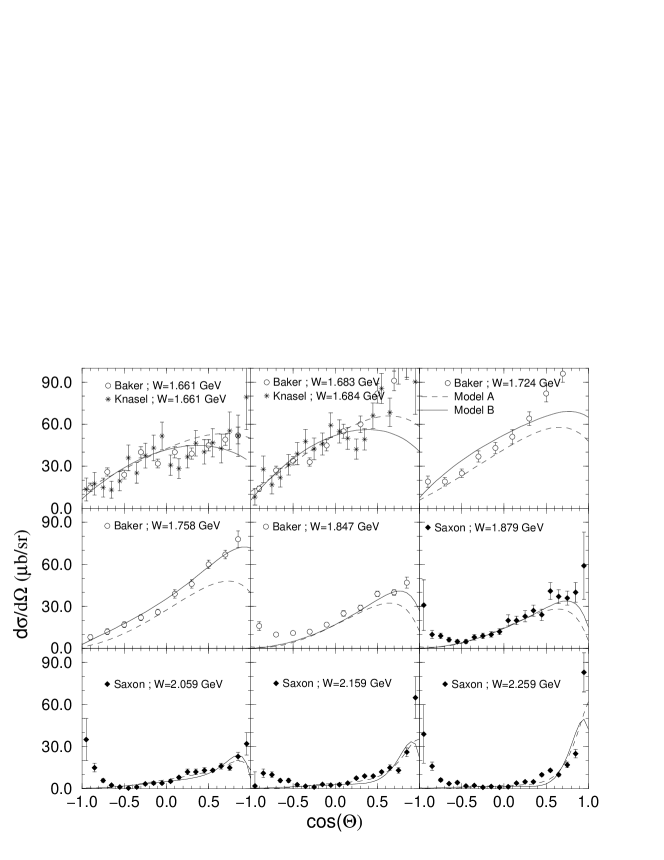
Figure 4: Differential cross-section for the reaction $\pi^{-}p\to K^{\circ}\Lambda$. The curves are from models A (dashed curves) and B (full curves). Data are from Refs. Bak78L ; Kna75 .

For the $\pi^{-}p\to K^{\circ}\Sigma^{\circ}$ reaction, the situation is different: the model B shows a significantly better agreement with the data up to $W\approx$ 2.1 GeV. At the two highest energies, models A and B produce comparable results and they both miss the bump around $\cos(\theta)\approx$ 0.3.

The main gross features of our results might be explained by the ingredients of the reaction mechanisms in our models. The $K^{\circ}\Lambda$ channel is dominated by the $N^{*}$ resonances. In our models the included resonances are around M $\approx$ 1.7 GeV. To cure the above short comings, we probably need to include higher mass resonances, especially the $P_{13}$(1900). This hypothesis is endorsed by the results reported in Ref. PM1 . In the case of the $K^{\circ}\Sigma^{\circ}$ channel, the $\Delta$ resonances embodied in our models are around M $\approx$ 1.9 GeV and ensure a much better reproduction of the data.

We have noticed that by loosening the constraints on the adjustable parameters ($\pm 3\delta$ instead of $\pm 2\delta$), the model-data agreement gets improved for the $K^{\circ}\Lambda$ channel, especially at backward angles. However, we feel that the extracted values are less meaningful.

Interpretation of recent data from JLab JLab and ELSA ELSA within a constituent quark model is in progress Sagxy . That work will allow us to determine the most pertinent resonances with respect to strangeness electromagnetic production. Afterwards, the present formalism will be used to imbed those resonances into planned future coupled-channel investigations of associated strangeness photo- and electro-production.

Figure 5: Differential cross-section for the reaction $\pi^{-}p\to K^{\circ}\Sigma^{\circ}$. The curves are as in Fig. (4). Data are from Refs. Bak78S ; Har80 .

III.2 Polarization asymmetry for $\pi^{-}p\to K^{\circ}\Lambda,~{}K^{\circ}\Sigma^{\circ}$ processes

The quality of the final state hyperon polarization asymmetry data, shown in Figs. 6 and 7 is clearly very poor. Nevertheless, as already noticed by the Giessen Group PM1 , the inclusion of those data in the fitting procedure has a significant effect on the extracted coupling constants reported in Tables II and III.

Figure 6: $\Lambda$-polarization asymmetries for the reaction $\pi^{-}p\to K^{\circ}\Lambda$. The curves are as in Fig. (4). Data are from Refs. Bak78L ; Sax80 .

The main features of the polarized $\Lambda$ asymmetries (Fig. (6)) are that they are large and positive up to $W\approx$ 1.8 GeV, and above they show nodal structures. The model B shows a better agreement with the data at lower energies. The short comings at higher energies could again be attributed to the lack of higher mass $N^{*}$s in our models.

The most noticeable differences between models A and B are in the shapes of the $\Sigma-$ polarization asymmetry for $W\leq$  1.8 GeV (Fig. 7). The higher mass $\Delta$ resonances seem to play a less important role here than in the case of the differential cross-sections (Fig. 5).

Figure 7: $\Sigma$-polarization asymmetries for the reaction $\pi^{-}p\to K^{\circ}\Sigma^{\circ}$. The curves are as in Fig. (4). Data are from Ref. Har80 .

III.3 Role of the nucleon resonances in the reactions $\pi^{-}p\to K^{\circ}\Lambda,K^{\circ}\Sigma^{\circ}$.

It is interesting to identify the role of nucleon resonances within our model B. To do so, we have turned off the nucleon resonances, one at a time, by putting the relevant couplings in Table II to zero, and have calculated the observable without any readjustment of the other parameters. The excitation functions, at three angles, for the cross-sections and the polarization asymmetries are depicted in Figures (8) and (9) for the reactions $\pi^{-}p\rightarrow K^{\circ}\Lambda\ {\rm and}\ K^{\circ}\Sigma^{\circ}$, respectively.

The notation used in the figures for the resonances are those in Table II; namely, N4: $S_{11}(1650)$, N5: $D_{13}(1700)$, N6: $P_{11}(1710)$, and N7: $P_{13}(1720)$.

The most striking feature here is the angular dependence of the role played by each resonance.

In the $K^{\circ}\Lambda$ channel (Fig. 8, left column), the effects on the differential cross-sections due to the $S_{11}(1650)$ goes from highly dominant at forward angles to marginal at large backward angles.

For the P-wave resonances, $P_{11}(1710)$ and $P_{13}(1720)$, we observe strong effects at extreme angles, which also reveal large interference phenomena.

The D-Wave resonance, $D_{13}(1700)$, has a significant effect only below $\approx$ 1.7 GeV and show a sharp increase at intermediate and large angles. The possible role played by D-wave resonances has not been investigated in other recent works Car00 ; PM1 .

Figure 8: Excitation function at three angles for the reaction $\pi^{-}p\to K^{\circ}\Lambda$ from threshold up to W=2.3 GeV. The curves are from model B (full curve), and the same model without one nucleon resonance: N4 (dotted), N5 (dashed), N6 (long dashed), N7 (dash-dotted).

The polarized $\Lambda$ asymmetries (Fig. 8, right column), show very different behavior. At the forward angles, different resonances have comparable effects. Around 90^∘, the spin 3/2 resonances, $D_{13}(1700)$ and $P_{13}(1720)$, produce important interferences effects. Finally, at large backward angles, all resonances show significant contributions below $\approx$ 1.9 GeV.

The results of a similar study on the role of the resonances for the process $\pi^{-}p\to K^{\circ}\Sigma^{\circ}$ are depicted in Fig. 9.

Here the $S_{11}(1650)$ resonance has a significant effect on both observables and at all angles. The $P_{11}(1710)$ shows small contributions in the whole phase space for both observables, while the other P-wave with higher spin, $P_{13}(1720)$, produces significant effects at forward angles in the differential cross-section below W $\approx$ 2.0 GeV, and even more at large backward angles. The role played by the D-Wave resonance, $D_{13}(1700)$, in the differential cross-section increases with angle and becomes comparable to that of $S_{11}(1650)$ at large backward angles. Finally, the polarization observable does not show any significant sensitivity to the $P_{13}(1720)$ and $D_{13}(1700)$ resonances.

Such a partial-wave decomposition has been also performed by the Giessen Group PM1 on the total cross-section observables, leading also to small contributions from the $P_{11}$ resonances. Effects found there for the other three resonances are compatible with our findings.

Finally, we have performed a similar decomposition for the $\Delta$ resonances included in our model B. However, no note-worthy effect was observed.

Figure 9: Same as Fig. (8), but for the $\pi^{-}p\to K^{\circ}\Sigma^{\circ}$ channel.

III.4 Total cross section for the reactions $\pi^{-}p\to K^{\circ}\Lambda$ and $\pi^{-}p\to K^{\circ}\Sigma^{\circ}$

Total cross-section data were not included in our fitting data-base. Our results are hence, postdictions.

For the reaction $\pi^{-}p\to K^{\circ}\Lambda$ the two models give comparable results, and model B does slightly better at lower energies.

In the case of $\pi^{-}p\to K^{\circ}\Sigma^{\circ}$ channel the situation is very different: model B gives a significantly better agreement with the data than does model A.

Both features reflect our comments about the differential cross-sections, showing that the method used to extracted total cross-section data from differential cross-section measurements is sufficiently reliable.

Figure 10: Total cross section for the reactions $\pi^{-}p\to K^{\circ}\Lambda$ (upper box), and $\pi^{-}p\to K^{\circ}\Sigma^{\circ}$ (lower box). Curves are the same as in Fig. (4). Data are from Refs. Bak78L ; Kna75 ; Sax80 ; Har80 .

III.5 Total cross sections of $KY\rightarrow KY$ processes

Using the models we have constructed, one can predict the $KY\rightarrow KY$ amplitudes. These amplitudes, although presently inaccessible experimentally, are needed for dynamical coupled-channel investigations of the electromagnetic production of hyperons. As an example, we show in Fig. 11 the predicted total cross sections for the $K^{\circ}\Lambda\to K^{\circ}\Lambda$, $K^{\circ}\Lambda\to K^{\circ}\Sigma^{\circ}$, and $K^{\circ}\Sigma^{\circ}\to K^{\circ}\Sigma^{\circ}$ processes.

For each of the models, we show two curves: i) contributions due only to the resonant terms (dotted curve for model A and dash-dotted for model B), ii) full calculation (dashed curves for model A and full curves for model B).

Figure 11: Total cross section for the reactions $K^{\circ}\Lambda\to K^{\circ}\Lambda$ (upper box), $K^{\circ}\Lambda\to K^{\circ}\Sigma^{\circ}$ (middle box), and $K^{\circ}\Sigma^{\circ}\to K^{\circ}\Sigma^{\circ}$ (lower box). Curves come from only resonant terms for models A and B (dotted and dash-dotted, respectively, and full A and B models (dashed and full curves, respectively).

We see that the predictions from model A and model B are strikingly different. Within model B, the resonant terms play a more significant role in all three channels. Moreover, the magnitude of the total cross sections are higher by roughly a factor of 4 for model B than for model A.

We therefore expect that the more realistic model B will generate very different final state $KY$ scattering effects on Kaon electromagnetic production reactions. Our investigations in this direction will be published elsewhere.

IV Summary and Conclusions

Based on an extension of the dynamical model of Ref. Sat96 , we have developed an approach to construct the coupled-channel models for describing the $\pi N\rightarrow KY$ and $KY\rightarrow KY$ reactions at energies where the baryon resonances are strongly excited. As a start, we only consider $\pi N$ and $KY$ ($\equiv~{}K\Lambda$, $K\Sigma$) channels. Furthermore, the resonances which were found to be important in the $\pi N\to KY$ and kaon photoproduction reactions are included in the investigations. Thus the models we construct can be consistently used to also investigate kaon electromagnetic production reactions. Undoubtedly, our objective is very limited compared to a more rigorous coupled-channel approach, which necessarily includes more channels, such as $\pi\Delta$, $\rho N$, and $\omega N$. However, our approach can be used to include additional nucleon and hyperon resonances with spin $\leq$ 3/2.

Given that no attempt is made to also fit the $\pi N$ elastic scattering data, we solve the coupled-channel equations with a simplification that the $\pi N\rightarrow\pi N$ scattering t-matrix elements are parameterized in terms of the empirical $\pi N$ partial-wave amplitudes and a phenomenological off-shell function. On the other hand, the basic non-resonant $\pi N\rightarrow KY$ and $KY\rightarrow KY$ transition potentials are derived rigorously from effective Lagrangians using a unitary transformation method.

We have constructed two models. The first one (model A) is built by assuming that all coupling constants and resonance parameters can be fixed using SU(3)-symmetry information from the Particle Data Group, plus values from a constituent quark model. The second model (B) is obtained by allowing most of the parameters to vary around the values of model A in fitting the data. Good fits to the available differential cross section and spin observable data for $\pi^{-}p\to K^{\circ}\Lambda,~{}K^{\circ}\Sigma^{\circ}$ have been achieved. The investigated kinematics region in the center-of-mass frame goes from threshold to 2.5 GeV.

The constructed models will facilitate coupled-channel studies of kaon photo- and electro-production reactions. In particular, the predicted $KY\rightarrow KY$ amplitudes, which are inaccessible experimentally, are needed to predict coupled-channel effects, such as that due to the $\gamma N\rightarrow K\Lambda\rightarrow K\Sigma$ transition. Our effort in this direction will be published elsewhere.

Appendix A LAGRANGIANS

The effective Lagrangians used in this work are given in this appendix for reference.

A.1 Born term interaction

The $0^{-}$meson-$\frac{1}{2}^{+}$baryon interactions are usually described using either pseudoscalar(PS) or pseudovector (PV) coupling,

$${\cal L}_{MBB^{\prime}}^{(PS)} = -ig_{MBB^{\prime}}\,\bar{\psi}\,\gamma_{5}\,\psi^{\prime}\,\phi\,+\,h.c.\,,$$ (39)

$${\cal L}_{MBB^{\prime}}^{(PV)} = -\frac{f_{MBB^{\prime}}}{m_{\pi}}\,\bar{\psi}\,\gamma_{5}\,\gamma_{\mu}\,\psi^{\prime}\,\partial^{\mu}\phi\,+\,h.c.\,.$$ (40)

If baryons $B$ and $B^{\prime}$ are on-shell, then ${\cal L}_{MBB^{\prime}}^{(PS)}$ and ${\cal L}_{MBB^{\prime}}^{(PV)}$ are equivalent, and the pseudoscalar coupling $g_{MBB^{\prime}}$ and pseudovector coupling $f_{MBB^{\prime}}$ are related by

$$\frac{f_{MBB^{\prime}}}{m_{\pi}}=\frac{g_{MBB^{\prime}}}{M_{B}+M_{B^{\prime}}}\,.$$ (41)

In this work, the pseudovector coupling is used for both $\pi$ and $K$ sectors. Using SU(3) symmetry as discussed later, we can express the interaction Lagrangians in each particle basis. For example, the Lagrangian for the ($K^{+}p\,\Lambda$) vertex can be written as

$${\cal L}_{K^{+}p\,\Lambda}^{(PV)}=-\frac{f_{K\Lambda N}}{m_{\pi}}\Bigl{(}\,\bar{p}\,\gamma_{5}\gamma_{\mu}\,\Lambda\,\partial^{\mu}K^{+}+\bar{\Lambda}\,\gamma_{5}\gamma_{\mu}\,p\,\partial^{\mu}\bar{K}^{-}\Bigr{)}\ ,$$

where the field operators are denoted by the particle’s identity.

A.2 SU(3) symmetry

The notation used to described the particle fields is defined here:

$$N\equiv\left(\begin{array}[]{c}p\\ n\end{array}\right),\qquad\bar{N}\equiv\bigl{(}\bar{p},\;\bar{n}\bigr{)}.$$ (42)

$$K\equiv\left(\begin{array}[]{c}K^{+}\\ K^{0}\end{array}\right),\qquad\bar{K}\equiv\bigl{(}K^{-},\;\bar{K^{0}}\bigr{)}.$$ (43)

$$\bm{\tau}\cdot\bm{\pi}\equiv\left(\begin{array}[]{cc}\pi^{0}&\sqrt{2}\pi^{+}\\ \sqrt{2}\pi^{-}&-\pi^{0}\end{array}\right).$$ (44)

$$\bm{\tau}\cdot\bm{\Sigma}\equiv\left(\begin{array}[]{cc}\Sigma^{0}&\sqrt{2}\Sigma^{+}\\ \sqrt{2}\Sigma^{-}&-\Sigma^{0}\end{array}\right),\qquad\bar{\bm{\Sigma}}\cdot\bm{\tau}\equiv\left(\begin{array}[]{cc}\bar{\Sigma}^{0}&\sqrt{2}\bar{\Sigma}^{-}\\ \sqrt{2}\bar{\Sigma}^{+}&-\bar{\Sigma}^{0}\end{array}\right).$$ (45)

$$\Delta\equiv\left(\begin{array}[]{c}\Delta^{++}\\ \Delta^{+}\\ \Delta^{0}\\ \Delta^{-}\end{array}\right),\qquad\bar{\Delta}\equiv\bigl{(}\bar{\Delta}^{++},\;\bar{\Delta}^{+},\;\bar{\Delta}^{0},\;\bar{\Delta}^{-}\bigr{)}.$$ (46)

Suppressing the factors $\gamma_{5}\gamma_{\mu}\partial^{\mu}$ for $PV$ coupling (or $i\gamma_{5}$ for $PS$ coupling), the explicit interaction Lagrangians in the SU(3) sector for octet baryons are:

$$\begin{split}{\cal L}_{\pi NN}=&-\frac{f_{\pi NN}}{m_{\pi}}\,\bar{N}\bm{\tau}N\cdot\bm{\pi}\\ =&-\frac{f_{\pi NN}}{m_{\pi}}\Bigl{[}\,\bar{p}\,p\,\pi^{0}-\bar{n}\,n\,\pi^{0}+\sqrt{2}\,\bar{p}\,n\,\pi^{+}+\sqrt{2}\,\bar{n}\,p\,\pi^{-}\Bigr{]}\,,\\[10.00002pt] {\cal L}_{\pi\Lambda\Sigma}=&-\frac{f_{\pi\Lambda\Sigma}}{m_{\pi}}\,\bigl{(}\bar{\Lambda}\bm{\Sigma}+\bar{\bm{\Sigma}}\Lambda\bigr{)}\cdot\bm{\pi}\\ =&-\frac{f_{\pi\Lambda\Sigma}}{m_{\pi}}\Bigl{[}\,\bar{\Lambda}\,(\Sigma^{+}\pi^{-}+\Sigma^{0}\pi^{0}+\Sigma^{-}\pi^{+})+(\bar{\Sigma}^{+}\pi^{+}+\bar{\Sigma}^{0}\pi^{0}+\bar{\Sigma}^{-}\pi^{-})\,\Lambda\,\Bigr{]}\,,\\[10.00002pt] {\cal L}_{\pi\Sigma\Sigma}=&\,\ i\ \frac{f_{\pi\Sigma\Sigma}}{m_{\pi}}\,\bigl{(}\bar{\bm{\Sigma}}\times\bm{\Sigma}\bigr{)}\cdot\bm{\pi}\\ =&-\frac{f_{\pi\Sigma\Sigma}}{m_{\pi}}\Bigl{[}(\bar{\Sigma}^{+}\Sigma^{+}-\bar{\Sigma}^{-}\Sigma^{-})\,\pi^{0}+(\bar{\Sigma}^{0}\Sigma^{-}-\bar{\Sigma}^{+}\Sigma^{0})\,\pi^{+}+(\bar{\Sigma}^{-}\Sigma^{0}-\bar{\Sigma}^{0}\Sigma^{+})\,\pi^{-}\Bigr{]}\,,\\[10.00002pt] {\cal L}_{K\Lambda N}=&-\frac{f_{K\Lambda N}}{m_{\pi}}\Bigl{[}\,\bar{\Lambda}\,(\bar{K}N)+(\bar{N}K)\,\Lambda\,\Bigr{]}\\ =&-\frac{f_{K\Lambda N}}{m_{\pi}}\Bigl{[}(\bar{p}\,K^{+}+\bar{n}\,K^{0})\,\Lambda+\bar{\Lambda}\,(K^{-}p+\bar{K}^{0}n)\Bigr{]}\,,\\[10.00002pt] {\cal L}_{K\Sigma N}=&-\frac{f_{K\Sigma N}}{m_{\pi}}\Bigl{[}\,\bar{\bm{\Sigma}}\cdot(\bar{K}\bm{\tau}N)+(\bar{N}\bm{\tau}K)\cdot{\bm{\Sigma}}\,\Bigr{]}\\ =&-\frac{f_{K\Sigma N}}{m_{\pi}}\Bigl{[}\;\bar{\Sigma}^{0}(K^{-}p-\bar{K}^{0}n)+\sqrt{2}\,\bar{\Sigma}^{+}K^{0}p+\sqrt{2}\,\bar{\Sigma}^{-}K^{-}n\\ &\phantom{-\frac{f_{K\Sigma N}}{m_{\pi}}\Bigl{[}\,}+(\bar{p}\,K^{+}-\bar{n}\,K^{0})\,\Sigma^{0}+\sqrt{2}\,\bar{p}\,K^{0}\Sigma^{+}+\sqrt{2}\,\bar{n}\,K^{+}\Sigma^{-}\Bigr{]}\,.\end{split}$$ (47)

For interactions involving the $\Delta$, which is a decuplet baryon with isospin $3/2$ , the Lagrangians are

$$\begin{split}{\cal L}_{\pi N\Delta}=&\frac{f_{\pi N\Delta}}{m_{\pi}}\Bigl{[}\,\bar{\Delta}^{\mu}\,\bm{T}\,N+\bar{N}\,\bm{T}^{\dagger}\Delta^{\mu}\Bigr{]}\cdot\partial_{\mu}\bm{\pi}\,,\\ =&\frac{f_{\pi N\Delta}}{m_{\pi}}\Bigl{[}\,-\bar{\Delta}^{++}\pi^{+}p+\bar{\Delta}^{+}\bigr{(}\sqrt{\tfrac{2}{3}}\,\pi^{0}p-\sqrt{\tfrac{1}{3}}\,\pi^{+}n\bigr{)}\\ &\phantom{\frac{f_{\pi N\Delta}}{m_{\pi}}\Bigl{[}\,}+\bar{\Delta}^{0}\bigr{(}\sqrt{\tfrac{1}{3}}\,\pi^{-}p+\sqrt{\tfrac{2}{3}}\,\pi^{0}n\bigr{)}\,+\bar{\Delta}^{-}\pi^{-}n+h.c.\,\Bigr{]}\,,\\[10.00002pt] {\cal L}_{K\Sigma\Delta}=&\frac{f_{K\Sigma\Delta}}{m_{\pi}}\Bigl{[}\,\bar{\Delta}^{\mu}\,\bm{T}\cdot{\bm{\Sigma}}\;\partial_{\mu}K+\partial_{\mu}\bar{K}\,\bar{\bm{\Sigma}}\cdot\bm{T}\,\Delta^{\mu}\Bigr{]}\\ =&\frac{f_{K\Sigma\Delta}}{m_{\pi}}\Bigl{[}\,-\bar{\Delta}^{++}\Sigma^{+}K^{+}+\bar{\Delta}^{+}\bigr{(}\sqrt{\tfrac{2}{3}}\,\Sigma^{0}K^{+}-\sqrt{\tfrac{1}{3}}\,\Sigma^{+}K^{0}\bigr{)}\\ &\phantom{\frac{f_{K\Sigma\Delta}}{m_{\pi}}\Bigl{[}\,}+\bar{\Delta}^{0}\bigr{(}\sqrt{\tfrac{1}{3}}\,\Sigma^{-}K^{+}+\sqrt{\tfrac{2}{3}}\,\Sigma^{0}K^{0}\bigr{)}\,+\bar{\Delta}^{-}\Sigma^{-}K^{0}+h.c.\,\Bigr{]}\,,\end{split}$$ (48)

where the four-vector indices and derivatives are suppressed in the second lines. The couplings in Eqs.(47-48) can be related using SU(3) symmetry Sto97 .

A.3 Baryon resonance interaction

The general interaction Lagrangians for baryon resonances (for spin-1/2 and 3/2) are described here. As in the Born terms, the explicit form for each SU(3) sector can be obtained by making appropriate substitutions in Eqs.(47-48),

$$\begin{split}{\cal L}_{MBR(\frac{1}{2}^{\pm})}^{(PS)}=&-g_{MBR}\,\bar{R}\,\Gamma\,\psi\,\phi\,+\,h.c.\,,\\[5.0pt] \mbox{with}\ \Gamma\equiv&\left\{\begin{array}[]{cl}i\gamma_{5}&\mbox{for $R(\frac{1}{2}^{+})$}\\ 1&\mbox{for $R(\frac{1}{2}^{-})$}\end{array}\right..\end{split}$$ (49)

$$\begin{split}{\cal L}_{MBR(\frac{1}{2}^{\pm})}^{(PV)}=&-\frac{f_{MBR}}{m_{\pi}}\,\bar{R}\,\Gamma_{\mu}\,\psi\,\partial^{\mu}\phi\,+\,h.c.\,,\\[5.0pt] \mbox{with}\ \Gamma_{\mu}\equiv&\left\{\begin{array}[]{cl}\gamma_{5}\gamma_{\mu}&\mbox{for $R(\frac{1}{2}^{+})$}\\ i\gamma_{\mu}&\mbox{for $R(\frac{1}{2}^{-})$}\end{array}\right..\end{split}$$ (50)

where the pseudovector couplings $f_{MBR}$ and the pseudoscalar couplings $g_{MBR}$ for resonance $R(\frac{1}{2}^{\pm})$ are related by

$$\frac{f_{MBR}}{m_{\pi}}=\frac{g_{MBR}}{M_{R}\pm M_{B}}\,.$$ (51)

$$\begin{split}{\cal L}_{MBR(\frac{3}{2}^{\pm})}=&\,\frac{f_{MBR}}{m_{\pi}}\,\Bigl{[}\,\bar{R}^{\mu}\,\Gamma\,\Theta_{\mu\nu}(Z)\,\psi\,\partial^{\nu}\phi+\bar{\psi}\,\Gamma\,\Theta_{\nu\mu}(Z)\,R^{\mu}\,\partial^{\nu}\phi^{\dagger}\,\Bigr{]}\,,\\[5.0pt] &\mbox{with}\ \Gamma\equiv\left\{\begin{array}[]{cl}1&\mbox{for $R(\frac{3}{2}^{+})$}\\ i\gamma_{5}&\mbox{for $R(\frac{3}{2}^{-})$}\end{array}\right.,\\[5.0pt] &\mbox{and}\ \Theta_{\mu\nu}(Z)\equiv g_{\mu\nu}-(Z+\frac{1}{2})\gamma_{\mu}\gamma_{\nu}\,.\end{split}$$ (52)

A.4 Vector meson interaction

For vector meson interactions, the corresponding Lagrangians are:

$$\begin{split}{\cal L}_{K^{*}YN}^{(V)}=&-g^{V}_{K^{*}\Lambda N}\bigl{(}\bar{N}\gamma^{\mu}\,\Lambda\,K^{*}_{\mu}+\bar{K}^{*}_{\mu}\,\bar{\Lambda}\,\gamma^{\mu}N\bigr{)}\\ &-g^{V}_{K^{*}\Sigma N}\bigl{(}\bar{N}\gamma^{\mu}\,\bm{\tau}\cdot\bm{\Sigma}\,K^{*}_{\mu}+\bar{K}^{*}_{\mu}\,\bar{\bm{\Sigma}}\cdot\bm{\tau}\,\gamma^{\mu}N\bigr{)}\,,\\[10.00002pt] {\cal L}_{K^{*}YN}^{(T)}=&-\frac{g^{T}_{K^{*}\Lambda N}}{M_{\Lambda}+M_{N}}\bigl{(}\bar{N}\sigma^{\mu\nu}\Lambda\,\partial_{\mu}K^{*}_{\nu}+\partial_{\mu}\bar{K}^{*}_{\nu}\,\bar{\Lambda}\,\sigma^{\mu\nu}N\bigr{)}\\ &-\frac{g^{T}_{K^{*}\Sigma N}}{M_{\Sigma}+M_{N}}\bigl{(}\bar{N}\sigma^{\mu\nu}\bm{\tau}\cdot\bm{\Sigma}\,\partial_{\mu}K^{*}_{\nu}+\partial_{\mu}\bar{K}^{*}_{\nu}\,\bar{\bm{\Sigma}}\cdot\bm{\tau}\,\sigma^{\mu\nu}N\bigr{)}\,,\\[10.00002pt] {\cal L}_{K_{1}YN}^{(V)}=&-i\,g^{V}_{K_{1}\Lambda N}\bigl{(}\bar{N}\gamma^{\mu}\gamma_{5}\,\Lambda\,K^{*}_{\mu}+\bar{K}^{*}_{\mu}\,\bar{\Lambda}\,\gamma_{5}\gamma^{\mu}N\bigr{)}\\ &-i\,g^{V}_{K_{1}\Sigma N}\bigl{(}\bar{N}\gamma^{\mu}\gamma_{5}\,\bm{\tau}\cdot\bm{\Sigma}\,K^{*}_{\mu}+\bar{K}^{*}_{\mu}\,\bar{\bm{\Sigma}}\cdot\bm{\tau}\,\gamma_{5}\gamma^{\mu}N\bigr{)}\,,\\[10.00002pt] {\cal L}_{K_{1}YN}^{(T)}=&-\frac{i\,g^{T}_{K_{1}\Lambda N}}{M_{\Lambda}+M_{N}}\bigl{(}\bar{N}\sigma^{\mu\nu}\gamma_{5}\,\Lambda\,\partial_{\mu}K^{*}_{\nu}+\partial_{\mu}\bar{K}^{*}_{\nu}\,\bar{\Lambda}\,\gamma_{5}\sigma^{\mu\nu}N\bigr{)}\\ &-\frac{i\,g^{T}_{K_{1}\Sigma N}}{M_{\Sigma}+M_{N}}\bigl{(}\bar{N}\sigma^{\mu\nu}\gamma_{5}\,\bm{\tau}\cdot\bm{\Sigma}\,\partial_{\mu}K^{*}_{\nu}+\partial_{\mu}\bar{K}^{*}_{\nu}\,\bar{\bm{\Sigma}}\cdot\bm{\tau}\,\gamma_{5}\sigma^{\mu\nu}N\bigr{)}\,.\end{split}$$

Appendix B Coupling constants

B.1 Hadronic couplings

In Sec. A.3, we give the interaction Lagrangians ${\cal L}_{MBR}$ for spin-1/2 and 3/2 baryon resonances $R$ ($=N^{*},\,\Delta^{*},\,Y^{*}$), where $B=N,\,\Delta,\,Y$ and $M=\pi,\,K$. The coupling constants in Eqs. (49-52) can be derived from partial widths $\Gamma$ in the decay $R\rightarrow MB$. The derivation is straightforward, and the formulae are given here:
For resonances with $J^{P}=1/2^{\pm}$,

$$\Gamma_{1/2^{\pm}} = C_{\mathrm{iso}}\,\frac{g_{MBR}^{2}}{4\pi}\,\frac{E_{B}\mp M_{B}}{M_{R}}\;q\,,$$ (53)

$$= C_{\mathrm{iso}}\,\frac{f_{MBR}^{2}}{4\pi}\left(\frac{M_{R}\pm M_{B}}{m_{\pi}}\right)^{2}\frac{E_{B}\mp M_{B}}{M_{R}}\;q\,,$$

and for resonances with $J^{P}=3/2^{\pm}$,

$$\Gamma_{3/2^{\pm}}=C_{\mathrm{iso}}\,\frac{f_{MBR}^{2}}{12\pi m_{\pi}^{2}}\,\frac{E_{B}\pm M_{B}}{M_{R}}\;q^{3}\,,$$ (54)

where $E_{B}$ is the energy of the final baryon, and $q$ denotes the three-momentum of the meson and baryon in the rest frame of the decaying resonance. $C_{\mathrm{iso}}$ is the isospin factor, and $C_{\mathrm{iso}}=3$ for decays $N^{*}\rightarrow\pi N$ and $N^{*}\rightarrow K\Sigma$, and $C_{\mathrm{iso}}=1$ otherwise.

B.2 $KYN$ and $\pi YY$ couplings

In this Section we summarize the situation with respect to the free parameters $f_{K\Lambda N}~{},~{}f_{K\Sigma N}~{},~{}f_{\pi\Sigma\Lambda}$, and $f_{\pi\Sigma\Sigma}$, see Table II.

Given that in the literature pseudoscalar couplings are more commonly used, we would like to make clear the relation between those and the pseudovector ones used in our work.

B.2.1 Expressions

Actually the issues related to the use of pseudoscalar (PS) versus pseudovector (PV) couplings have been discussed by several authors (see, e.g. PSvPV ; seoul ), but at the present time there is no strong argument to prefer one to the other.

Using de Swart convention, we have the following relations for the PS couplings:

$$g_{K\Lambda N} = -\frac{g_{\pi NN}}{\sqrt{3}}~{}(3-2\alpha_{D}),$$ (55)

$$g_{K\Sigma N} = g_{\pi NN}~{}(2\alpha_{D}-1),$$ (56)

$$g_{\pi\Lambda\Sigma} = \frac{2}{\sqrt{3}}~{}\alpha_{D}~{}g_{\pi NN},$$ (57)

$$g_{\pi\Sigma\Sigma} = 2~{}(1-\alpha_{D})~{}g_{\pi NN},$$ (58)

with $\alpha_{D}=\frac{D}{D+F}$ the standard fraction of D- and F-couplings.

The relations between PV and PS couplings are (see e.g. seoul ; Loiseau :

$$f_{\pi NN} = \frac{m_{\pi}}{2M_{N}}~{}g_{\pi NN},$$ (59)

$$f_{K\Lambda N} = \frac{m_{K}}{M_{N}+M_{\Lambda}}~{}g_{K\Lambda N},$$ (60)

$$f_{K\Sigma N} = \frac{m_{K}}{M_{N}+M_{\Sigma}}~{}g_{K\Sigma N},$$ (61)

$$f_{\pi\Lambda\Sigma} = \frac{m_{\pi}}{M_{\Lambda}+M_{\Sigma}}~{}g_{\pi\Lambda\Sigma},$$ (62)

$$f_{\pi\Sigma\Sigma} = \frac{m_{\pi}}{2M_{\Sigma}}~{}g_{\pi\Sigma\Sigma}.$$ (63)

Expressions relating PS and PV couplings for $KNN^{*}$ and $KNY^{*}$, for S- and P-resonances, can be found in seoul .

B.2.2 Numerical considerations

The central values of two main KYN couplings are determined using Eqs. (B3) and (B4), with $\alpha_{D}=0.644$ (Ref. Don ), and $g_{\pi NN}=14.11$ (Ref. PiNN ). For those couplings, the allowed ranges in the fitting procedure are in line with the findings of a recent work General based on generalized Goldberger-Treiman relation combined with the Dashen-Weinstein sum rule, which puts the following uncertainties on the $g_{K\Lambda N}$ and $g_{K\Sigma N}$ couplings: $\pm 36\%$ and $\pm 55\%$, respectively. We hence find:

$$\frac{g_{K\Lambda N}}{\sqrt{4\pi}}=-3.934~{}~{};~{}~{}-5.351~{}\leq\frac{g_{K\Lambda N}}{\sqrt{4\pi}}~{}\leq~{}-2.518$$

$$\frac{g_{K\Sigma N}}{\sqrt{4\pi}}=1.146~{}~{};~{}~{}0.516~{}\leq\frac{g_{K\Sigma N}}{\sqrt{4\pi}}~{}\leq~{}1.777.$$

Finally, concerning the two other couplings, $\pi\Lambda\Sigma$ and $\pi\Sigma\Sigma$, the most recent works that we are aware of are Refs. Loiseau ; Doi but they do not give identical values.

References

- (1) W.-T. Chiang, F. Tabakin, T.-S. H. Lee, and B. Saghai, Phys. Lett. B517, 101 (2001).
- (2) T. Sato and T.-S. H. Lee, Phys. Rev. C 54, 2660 (1996).
- (3) D.S. Carman et al., The CLAS Collaboration, Phys. Rev. Lett. 90, 131804 (2003); J.W.C. McNabb et al., The CLAS Collaboration, submitted to Phys. Rev. Lett, nucl-ex/0305028.
- (4) K.H. Glander et al., Eur. Phys. J. A19, 251 (2004).
- (5) R.G.T. Zegers et al., Phys. Rev. Lett. 91, 092001 (2003).
- (6) O. Bartalini et al., Nucl. Phys. A699, 218 (2002).
- (7) See e.g., S. Capstick and W. Roberts, Prog. Part. Nucl. Phys. 45, 5241 (2002), and references therein.
- (8) B. Saghai and Z. Li, Eur. Phys. J. A11, 217 (2001); B. Saghai, AIP Conf. Proc. 59, 57 (2001), nucl-th/0105001.
- (9) B. Saghai, nucl-th/0310025.
- (10) N. Kaiser, T. Waas, and W. Weise, Nucl. Phys. A612, 297 (1997).
- (11) J. Caro Ramon, N. Kaiser, S. Wetzel, and W. Weise, Nucl. Phys. A672, 249 (2000).
- (12) B. Krippa, Phys. Rev. C 58, 1333 (1998).
- (13) J.A. Oller, E. Oset, and A. Ramos, Prog. Part. Nucl. Phys. 45, 157 (2000).
- (14) M.F.M. Lutz and E.E. Kolomeitsev, Nucl. Phys. A700, 193 (2002).
- (15) T. Hyodo, S. Nam, D. Jido, and A. Hosaka, Phys. Rev. C68, 018201 (2003).
- (16) T. Feuster and U. Mosel, Phys. Rev. C 58, 457 (1998).
- (17) A. Waluyo, C. Bennhold, H. Haberzettl, G. Penner, U. Mosel, and T. Mart, nucl-th/0008023.
- (18) G. Penner and U. Mosel, Phys. Rev. C 66, 055211 (2002).
- (19) G. Penner and U. Mosel, Phys. Rev. C 66, 055212 (2002).
- (20) A. Klein and T-S. H. Lee, Phys. Rev. D 10, 4308 (1974).
- (21) R. Blankenbecler and R. Sugar, Phys. Rev. 142, 1051 (1966).
- (22) F. Gross, Phys. Rev. C 26, 2203 (1982).
- (23) C.T. Hung, S.N. Yang, T.-S.H. Lee, J. Phys. G20, 1536 (1994).
- (24) B.D. Keister and W.N. Polyzou, Adv. Nucl. Phys. 20, 225 (1991).
- (25) T. Sato, M. Doi, N. Odagawa, and H. Ohtsubo, Few Body Syst. Suppl. 5, 254 (1992).
- (26) T. Sato, M. Kobayashi and H. Ohtsubo, unpublished.
- (27) R.D. Baker et al., Nucl. Phys. B141, 29 (1978).
- (28) R.D. Baker et al., Nucl. Phys. B145, 402 (1978).
- (29) T.M. Knasel et al., Phys. Rev. D 11, 1 (1975).
- (30) D.H. Saxon et al., Nucl. Phys. B162, 522 (1980).
- (31) J.C. Hart et al., Nucl. Phys. B166, 73 (1980).
- (32) B. Nelson et al., Phys. Rev. Lett. 31, 901 (1973); K.W. Bell et al., Nucl. Phys. B222, 389 (1983).
- (33) R.A. Arndt, I.I. Strakovsky, and R.L. Workman, Int. J. Mod. Phys. A18, 449 (2003).
- (34) http://gwdac.phy.gwu.edu.
- (35) See e.g., B. Saghai and F. Tabakin, Phys. Rev. C 53, 66 (1996), and references therein.
- (36) V. Shkylyar, G. Penner, U. Mosel, nucl-th/0403064.
- (37) K. Hagiwara et al.,Particle Data Group, Phys. Rev. D 66, 010001 (2002).
- (38) S. Capstick and W. Roberts, Phys. Rev. D 58, 074011 (1998).
- (39) R. Koniuk and N. Isgur, Phys. Rev. D 21,1868 (1980).
- (40) J.C. David, C. Fayard, G.H. Lamot, B. Saghai, Phys. Rev. C 53, 2613 (1996).
- (41) T. Mizutani, C. Fayard, G.H. Lamot, B. Saghai, Phys. Rev. C 58, 75 (1998).
- (42) T.E.O. Ericson, B. Loiseau, A.W. Thomas Phys. Rev. C 66, 014005 (2002).
- (43) V.G.J. Stocks and T.A. Rijken, Nucl. Phys. A613, 311 (1997).
- (44) C. Bennhold, L.E. Wright, Phys. Rev. C 36, 438 (1987); J. Cohen, Phys. Rev. C 37, 187 (1988); M.K. Cheoun, B.S. Han, B.G. Yu, Il-Tong Cheon, Phys. Rev. C 54, 1811 (1996); S.S. Hsiao, D.H. Lu, Shin Nan Yang, Phys. Rev. C 61, 068201 (2000).
- (45) Bong Soo Han, Myung Ki Cheoun, K.S. Kim, Il-Tong Cheon, Nucl. Phys. A691, 713 (2001).
- (46) B. Loiseau, S. Wycech Phys. Rev. C 63, 034003 (2001).
- (47) J.F. Donoghue, B.R. Holstein, Phys. Rev. D 25, 2015 (1982).
- (48) I.J. General, S.R. Cotanch, Phys. Rev. C 69, 035202 (2004).
- (49) T. Doi, Y. Kondo, M. Oka, hep-ph/031117.