Abstract

Fluctuations of charged particle number are studied in the canonical ensemble. In the infinite volume limit the fluctuations in the canonical ensemble are different from the fluctuations in the grand canonical one. Thus, the well-known equivalence of both ensembles for the average quantities does not extend for the fluctuations. In view of a possible relevance of the results for the analysis of fluctuations in nuclear collisions at high energies, a role of the limited kinematical acceptance is studied.

1. Introduction.   The statistical approach to strong interactions is surprisingly successful in describing experimental results on hadron production properties in nuclear collisions at high energies (see e.g. Ref. [1] and references therein). This motivates a rapid development of statistical models and it raises new questions, previously not addressed in statistical physics. In particular, an applicability of the models formulated within various statistical ensembles has been considered for average quantities. The micro-canonical ensemble, where the motional and material conservation laws are strictly fulfilled in all microscopic states of the system, has to be used for collisions in which a small number of particles is produced, like p+p interactions at low energies (see e.g. Ref. [2]). The canonical ensemble ($~{}c.e.~{}$), where only the material conservation laws are obeyed, is relevant for the systems with a large number of all produced particles, but a small number of carriers of conserved charges like electric charge, baryon number, strangeness or charm (see e.g. Ref. [3]). Finally, models formulated using grand canonical ensemble ($~{}g.c.e.~{}$) can be used when the number of carriers of conserved charge is large enough (see e.g. Ref. [4]). In the latter approach both material and motional conservation laws are relaxed and the mean values of conserved charges and energy are adjusted by introduction of chemical potentials and temperature, respectively.

The question of applicability of various statistical ensembles for the study of fluctuations of physical quantities has not been addressed up to now. In the text-books of statistical mechanics, the particle number fluctuations are considered in $g.c.e$ only. It is because the discussion is limited to the non-relativistic cases, so that in the $c.e.$ the particle number is fixed. However, in the relativistic case, relevant for the models of hadron production in high energy nuclear collisions, only conserved charges are fixed, and consequently the particle number fluctuates in both $c.e.$ and $g.c.e.$ .

The analysis of fluctuations is an important tool to study a physical system created in high energy nuclear collisions (see e.g. [5]). Recently, rich experimental data on fluctuations of particle production properties in nuclear collisions at high energies have been presented (see e.g. presentations at “Quark Matter 2004”). In particular, intriguing results concerning the particle number fluctuations in collisions of small nuclei at the CERN SPS have been shown [6]. These new results motivate our work, in which the particle number fluctuations are calculated in $c.e.$ and compared with those obtained in $g.c.e.$ . Finally, the possible influence of the limited experimental acceptance on observed fluctuations is studied.

2. Partition function in g.c.e. and c.e.   Let us consider the system which consists of one sort of positively and negatively charged particles (e.g. $\;\pi^{+}\;$ and $\;\pi^{-}\;$ mesons) with total charge equal to zero $\;Q=0\;$. In the case of the Boltzmann ideal gas (the interactions and quantum statistics effects are neglected) in the volume $V$ and at temperature $T$ the g.c.e. partition function reads:

$$Z_{g.c.e.}(V,T)\;=\;\sum_{N_{+}=0}^{\infty}\sum_{N_{-}=0}^{\infty}\;\frac{(\lambda_{+}z)^{N_{+}}}{N_{+}!}\;\frac{(\lambda_{-}z)^{N_{-}}}{N_{-}!}\;=\;\exp\left(\lambda_{+}z~{}+~{}\lambda_{-}z\right)~{}=~{}\exp(2z)~{}.$$ (1)

In Eq. (1) $\;z\;$ is a single particle partition function

$$z\;=\;\frac{V}{2\pi^{2}}\int_{0}^{\infty}k^{2}dk\;\exp\left[-~{}\frac{(k^{2}+m^{2})^{1/2}}{T}\right]\;=\;\frac{V}{2\pi^{2}}\;\;T\,m^{2}\,K_{2}\left(\frac{m}{T}\right)~{},$$ (2)

where $m$ is a particle mass and $\;K_{2}\;$ is the modified Hankel function. Parameters $\;\lambda_{+}\;$ and $\;\lambda_{-}\;$ are auxiliary parameters introduced in order to calculate the mean number and the fluctuations of positively and negatively charged particles (the chemical potential equals to zero to satisfy the condition $\langle Q\rangle_{g.c.e.}=0$). They are set to one in the final formulas.

The $c.e.$ partition function is obtained by an explicit introduction of the charge conservation constrain, $N_{+}-N_{-}=0$ for each microscopic state of the system and it reads:

$$Z_{c.e.}(V,T) \;=\;\sum_{N_{+}=0}^{\infty}\sum_{N_{-}=0}^{\infty}\;\frac{(\lambda_{+}z)^{N_{+}}}{N_{+}!}\;\frac{(\lambda_{-}z)^{N_{-}}}{N_{-}!}\;\delta(N_{+}-N_{-})\;=\;$$ (3)

$$\;=\;\frac{1}{2\pi}\int_{0}^{2\pi}d\phi\;\;\exp\left[z\;(\lambda_{+}\;e^{i\phi}\;+\;\lambda_{-}\;e^{-i\phi})\right]\;=\;I_{0}(2z)\;.$$

In Eq. (3) the integral representations of the $\delta$-Kronecker symbol and the modified Bessel function were used: [7]

$$\delta(n)=\frac{1}{2\pi}\int_{0}^{2\pi}d\phi~{}\exp(in\phi)~{},~{}~{}I_{Q}(2z)=\frac{1}{2\pi}\int_{0}^{2\pi}d\phi\;\exp[-iQ\phi\;+\;2z\;\cos\phi]\;.$$ (4)

3. Mean particle number.   The average number of $N_{+}$ and $N_{-}$ can be calculated as

$$\langle N_{\pm}\rangle\;=\;\left(\frac{\partial}{\partial\lambda_{\pm}}\ln Z\right)_{\lambda_{\pm}\;=\;1}~{},$$ (5)

and in the $\;g.c.e.\;$ (1) they are equal to:

$$\langle N_{\pm}\rangle_{g.c.e.}\;=\;\left(\frac{\partial}{\partial\lambda_{\pm}}\ln Z_{g.c.e.}\right)_{\lambda_{\pm}\;=\;1}=\;z~{}.$$ (6)

By construction the mean total charge is equal to zero: $\langle Q\rangle_{g.c.e.}=\langle N_{+}\rangle_{g.c.e.}-\langle N_{-}\rangle_{g.c.e.}=0$. In the c.e. (3) the charge conservation $Q=N_{+}-N_{-}=0$ is imposed on each microscopic state of the system. This condition introduces a correlation between particles which carry conserved charges. The average particle numbers are [3]:

$$\langle N_{\pm}\rangle_{c.e.}\;=\;\left(\frac{\partial}{\partial\lambda_{\pm}}\ln Z_{c.e.}\right)_{\lambda_{\pm}\;=\;1}\;=\;z\;\frac{I_{1}(2z)}{I_{0}(2z)}\;.$$ (7)

The exact charge conservation leads to the $\;c.e.\;$ suppression ($I_{1}(2z)/I_{0}(2z)<1$) of the charged particle multiplicity relative to the result for the $\;g.c.e.\;$ (6). The ratio of $\langle N_{\pm}\rangle$ calculated in the $~{}c.e.~{}$ and $~{}g.c.e.~{}$ is plotted as a function of $z$ in Fig. 1.

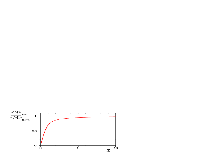
Figure 1: The ratio of $\langle N_{\pm}\rangle_{c.e.}$ (7) to $\langle N_{\pm}\rangle_{g.c.e.}$ (6) as a function of $z$.

In the large volume limit ($V\rightarrow\infty$ corresponds also to $z\rightarrow\infty$) the results for mean quantities in the $\;c.e.\;$ and $\;g.c.e.\;$ are equal. This result is referred as an equivalence of the canonical and grand canonical ensembles. It can be obtained using an asymptotic expansion of the modified Bessel function [7]:

$$\lim_{z\to\infty}I_{n}(2z)\;=\;\frac{\exp(2z)}{\sqrt{4\pi z}}\;\left[1~{}-~{}\frac{4n^{2}-1}{16z}~{}+~{}O\left(\frac{1}{z^{2}}\right)\right]~{},$$ (8)

which gives $I_{1}(2z)/I_{0}(2z)\rightarrow 1$ and therefore

$$\langle N_{\pm}\rangle_{c.e.}~{}\cong~{}\langle N_{\pm}\rangle_{g.c.e}=z~{}.$$ (9)

Using the series expansion one gets [7] for small systems ($z\ll 1$):

$$I_{n}(2z)~{}=~{}\frac{z^{n}}{n!}~{}+~{}\frac{z^{n+2}}{(n+1)!}~{}+~{}O\left(z^{n+4}\right)~{},$$ (10)

and consequently $I_{1}(2z)/I_{0}(2z)\cong z$ which results in

$$\langle N_{\pm}\rangle_{c.e.}~{}\cong~{}z^{2}~{}~{}\ll~{}~{}\langle N_{\pm}\rangle_{g.c.e.}~{}=~{}z~{}.$$ (11)

The asymptotics of the mean multiplicity discussed above are clearly seen in Fig. 1.

4. Scaled variance.   An useful measure of fluctuations of any variable $X$ is the ratio of its variance $V(X)=\langle X^{2}\rangle-\langle X\rangle^{2}$ to its mean value $\langle X\rangle$, referred here as the scaled variance:

$$\omega^{X}\;\equiv\;\frac{\langle X^{2}\rangle-\langle X\rangle^{2}}{\langle X\rangle}~{}.$$ (12)

Note, that $\omega^{X}=1$ for the Poisson distribution. Thus, to study the fluctuations of charged particles the second moment of the multiplicity distribution $\;\langle N_{\pm}^{2}\rangle\;$ has to be calculated. In the $~{}g.c.e.~{}$ (1) and $c.e.$ (3) one finds:

$$\langle N_{\pm}^{2}\rangle_{g.c.e.} \;=\;\frac{1}{Z_{g.c.e.}}\left[\frac{\partial}{\partial\lambda_{\pm}}\left(\lambda_{\pm}\frac{\partial\;\;Z_{g.c.e.}}{\partial\lambda_{\pm}}\right)\right]_{\lambda_{\pm}=1}\;=\;z\;+\;z^{2}~{},$$ (13)

$$\langle N_{\pm}^{2}\rangle_{c.e.} \;=\;\frac{1}{Z_{c.e.}}\left[\frac{\partial}{\partial\lambda_{\pm}}\left(\lambda_{\pm}\frac{\partial\;\;Z_{c.e.}}{\partial\lambda_{\pm}}\right)\right]_{\lambda_{\pm}=1}\;=\;z\;\frac{I_{1}(2z)}{I_{0}(2z)}\;+\;z^{2}\;\frac{I_{2}(2z)}{I_{0}(2z)}~{}=~{}z^{2}~{}.$$ (14)

The corresponding scaled variances are:

$$\omega_{g.c.e.}^{\pm} \;=\;\frac{\langle N_{\pm}^{2}\rangle_{g.c.e.}\;-\;\langle N_{\pm}\rangle_{g.c.e.}^{2}}{\langle N_{\pm}\rangle_{g.c.e.}}\;=\;1~{},$$ (15)

$$\omega_{c.e.}^{\pm} \;=\;\frac{\langle N_{\pm}^{2}\rangle_{c.e.}\;-\;\langle N_{\pm}\rangle_{c.e.}^{2}}{\langle N_{\pm}\rangle_{c.e.}}\;=\;1\;-\;z\left[\,\frac{I_{1}(2z)}{I_{0}(2z)}\;-\;\frac{I_{2}(2z)}{I_{1}(2z)}\,\right]~{}.$$ (16)

Using Eqs. (8) and (10) the asymptotic behaviour of $\omega_{c.e}^{\pm}$ for both $z\rightarrow 0$ and $z\rightarrow\infty$ can be found. The c.e. fluctuations measured in terms of $\omega$ are equal to those in the $~{}g.c.e.~{}$ for the small system ($z\ll 1$) (another variable to treat the fluctuations in the small systems is discussed in Appendix):

$$\omega_{c.e}^{\pm}\;\cong\;1~{}-~{}\frac{z^{2}}{2}\;\cong~{}1~{}=\omega^{\pm}_{g.c.e}~{}.$$ (17)

For large systems $(z\gg 1)$ the scaled variance for the $~{}c.e.~{}$ is two times smaller than the scaled variance for the $~{}g.c.e.~{}$:

$$\omega_{c.e.}^{\pm}\;\cong\;\frac{1}{2}~{}+~{}\frac{1}{8z}~{}\cong~{}\frac{1}{2}~{}=~{}\frac{1}{2}~{}\omega_{g.c.e.}^{{\pm}}\;.$$ (18)

The dependence of the scaled variance calculated within the $c.e$ and $g.c.e.$ on $z$ is shown in Fig. 2.

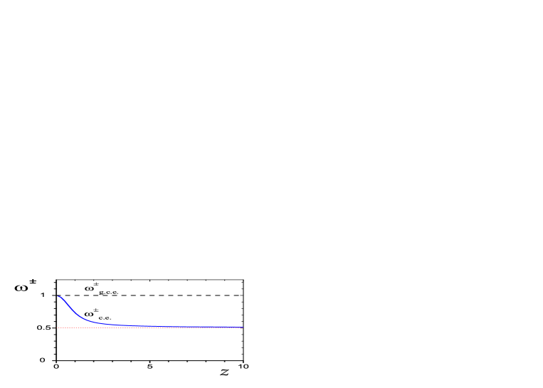
Figure 2: The scaled variances of $N_{\pm}$ calculated within the $~{}g.c.e.~{}$, $\omega^{\pm}_{g.c.e.}=1$ (15), and $~{}c.e.~{}$, $\omega^{\pm}_{c.e.}$ (16).

The scaled variance shows a very different behavior than the mean multiplicity. In the limit of small $z$ the ratio of the results for $c.e.$ and $g.c.e.$ approaches zero for the mean multiplicity (Fig. 1) and one for the scaled variance (Fig. 2). On the other hand in the large $z$ limit the mean multiplicity ratio approaches one and the scaled variance ratio 0.5. Thus in the case of fluctuations the canonical and grand canonical ensembles are not equivalent.

5. Multiplicity distribution.   In the $g.c.e.$ the multiplicity distribution of $\;N_{+}\;$ (and $\;N_{-}$) is equal to the Poisson one:

$$P_{g.c.e.}(N_{+})\; \equiv\;\sum_{N_{-}=0}^{\infty}~{}P_{g.c.e.}\left(N_{+},N_{-}\right)~{}=~{}\frac{1}{Z_{g.c.e.}}~{}\sum_{N_{-}=0}^{\infty}\frac{z^{N_{+}}}{N_{+}!}~{}\frac{z^{N_{-}}}{N_{-}!}$$ (19)

$$=~{}\exp(-z)\cdot\frac{z^{N_{+}}}{N_{+}!}~{},$$

whereas the corresponding distribution in the $\;c.e.\;$ (3) is:

$$P_{c.e.}(N_{+})\; \equiv\;\sum_{N_{-}=0}^{\infty}~{}P_{c.e.}\left(N_{+},N_{-}\right)~{}=~{}\frac{1}{Z_{c.e.}}~{}\sum_{N_{-}=0}^{\infty}\frac{z^{N_{+}}}{N_{+}!}~{}\frac{z^{N_{-}}}{N_{-}!}~{}\cdot\delta\left(N_{+}-N_{-}\right)$$ (20)

$$=\;\frac{1}{I_{0}(2z)}\cdot\left(\frac{z^{N_{+}}}{N_{+}!}\right)^{2}\;.$$

As an example, the distributions in $g.c.e.$ and $c.e.$ are plotted in Figs. 3 and 4 for $z=0.5$ (the small system) and $z=10$ (the large system), respectively.

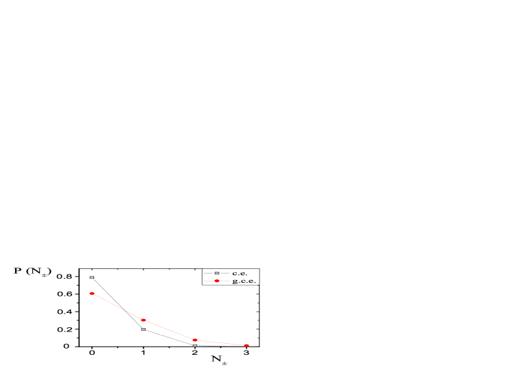
Figure 3: Multiplicity distributions $P_{c.e.}(N_{\pm})$ (20) and $P_{g.c.e.}(N_{\pm})$ (19) for $z=0.5$.

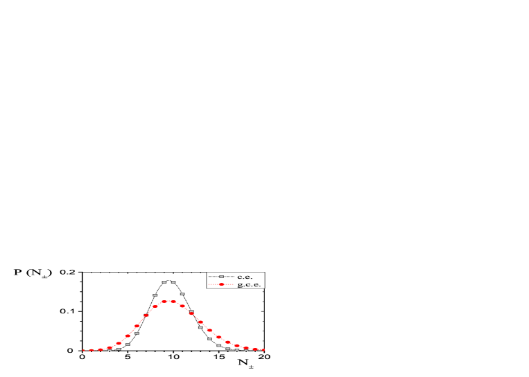
Figure 4: Multiplicity distributions $P_{c.e.}(N_{\pm})$ (20) and $P_{g.c.e.}(N_{\pm})$ (19) for $z=10$.

As expected from the previous discussion, the $~{}c.e.~{}$ distribution (20) is narrower (the variance is smaller) than the $~{}g.c.e.~{}$ one (19). This result is valid for both the large ($z\gg 1$) and the small ($z\ll 1$) system. On the other hand, the average value of $N_{\pm}$ is smaller in the $~{}c.e.~{}$ than in the $~{}g.c.e.~{}$ for small $z$. It results in $\omega^{\pm}_{c.e.}\rightarrow\omega^{\pm}_{g.c.e}=1$ at $z\rightarrow 0$. Moreover, for $\langle N_{\pm}\rangle\ll 1$ one can easily demonstrate that $\omega^{\pm}\cong 1$ for any $P(N_{\pm})$ distribution if the conditions $P(0)\gg P(1)\gg P(k)$ (with $k\geq 2$) are satisfied. Indeed, in this limit one can neglect all $P(N_{\pm})$ for $N_{\pm}\geq 2$ which results in:

$$\omega^{\pm}\;\equiv\;\frac{\langle N_{\pm}^{2}\rangle-\langle N_{\pm}\rangle^{2}}{\langle N_{\pm}\rangle}\;\cong\;\frac{P(1)\cdot 1^{2}\;-\;[P(1)\cdot 1]^{2}}{P(1)\cdot 1}\;\cong~{}1~{},$$ (21)

as $P(1)\cong\langle N_{\pm}\rangle\ll 1$. In the large volume limit, see Fig. 4, the mean values of the $c.e.$ and $g.c.e.$ distributions become equal, but the $c.e.$ distribution is narrower than the $g.c.e.$ one.

6. Total multiplicity of charged particles.   The total multiplicity of charged particles is defined as $N_{ch}=N_{+}+N_{-}$. Its average in the $\;g.c.e.\;$ and $~{}c.e.~{}$ reads:

$$\langle N_{ch}\rangle_{g.c.e.} \;=\;\langle\;N_{+}+N_{-}\;\rangle_{g.c.e.}\;=\;\langle N_{+}\rangle_{g.c.e.}+\langle N_{-}\rangle_{g.c.e.}\;=~{}2z\;,$$ (22)

$$\langle N_{ch}\rangle_{c.e.} \;=\;\langle\;N_{+}+N_{-}\;\rangle_{c.e.}\;=\;\langle N_{+}\rangle_{c.e.}+\langle N_{-}\rangle_{c.e.}\;=\;2z\;\frac{I_{1}(2z)}{I_{0}(2z)}\;.$$ (23)

In the $~{}g.c.e.~{}$ one finds:

$$\langle N_{ch}^{2}\rangle_{g.c.e.} ~{}=~{}\langle N_{+}^{2}+2N_{+}N_{-}+N_{-}^{2}\rangle_{g.c.e.}~{}=~{}\langle N_{+}^{2}\rangle_{g.c.e.}+2\langle N_{+}\rangle_{g.c.e.}\langle N_{-}\rangle_{g.c.e.}+$$ (24)

$$~{}+~{}\langle N_{-}^{2}\rangle_{g.c.e.}~{}=~{}z^{2}+z~{}+~{}2z^{2}~{}+~{}z^{2}+z~{}=~{}4z^{2}~{}+~{}2z~{},$$

and consequently the scaled variance of $N_{ch}$ in the $~{}g.c.e.~{}$ is:

$$\omega_{g.c.e.}^{ch}~{}\equiv~{}\frac{\langle N_{ch}^{2}\rangle_{g.c.e.}~{}-~{}\langle N_{ch}\rangle^{2}_{g.c.e.}}{\langle N_{ch}\rangle_{g.c.e.}}~{}=~{}\frac{4z^{2}+2z~{}-~{}(2z)^{2}}{2z}~{}=~{}1~{}.$$ (25)

The result (25) also follows from explicit expression on the probability distribution of $N_{ch}$ in the $~{}g.c.e.~{}$:

$$P_{g.c.e.}(N_{ch})~{}\equiv~{}\sum_{N_{+}}^{\infty}\sum_{N_{-}=0}^{\infty}P_{g.c.e.}\left(N_{+},N_{-}\right)\cdot\delta\left[N_{ch}-\left(N_{+}+N_{-}\right)\right]$$ (26)

$$~{}=~{}\frac{1}{Z_{g.c.e.}}~{}\sum_{N_{+}}^{\infty}\sum_{N_{-}=0}^{\infty}\frac{z^{N_{+}}}{N_{+}!}~{}\frac{z^{N_{-}}}{N_{-}!}\cdot\delta\left[N_{ch}-\left(N_{+}+N_{-}\right)\right]~{}=~{}\exp(-2z)~{}\frac{(2z)^{N_{ch}}}{N_{ch}!}~{}.$$

Thus distributions of $N_{ch}$ and $N_{\pm}$ are Poissonian in the $~{}g.c.e.~{}$. In the $~{}c.e.~{}$ the negatively and positively charged particles are correlated, $\langle N_{+}\cdot N_{-}\rangle_{c.e.}\neq\langle N_{+}\rangle_{c.e.}\cdot\langle N_{-}\rangle_{c.e.}$. The correlation term reads:

$$\langle N_{+}\cdot N_{-}\rangle_{c.e.}\;=\;\frac{1}{Z_{c.e.}}\left(\frac{\partial^{2}\;Z_{c.e.}}{\partial\lambda_{+}\partial\lambda_{-}}\right)_{\lambda_{\pm}=1}~{}=\;z^{2}~{}.$$ (27)

Using Eqs. (14) and (27) one obtains the scaled variance of $N_{ch}$ in the $~{}c.e.~{}$:

$$\omega_{c.e.}^{ch}\;\equiv~{}\frac{\langle N_{ch}^{2}\rangle_{c.e.}\;-\;\langle N_{ch}\rangle^{2}_{c.e.}}{\langle N_{ch}\rangle_{c.e.}}\;=\;1\;+\;z\left[\frac{I_{2}(2z)+I_{0}(2z)}{I_{1}(2z)}\;-\;2\;\frac{I_{1}(2z)}{I_{0}(2z)}\right]~{}.$$ (28)

The scaled variances $\omega^{ch}_{g.c.e}$ and $\omega^{ch}_{c.e.}$ as functions of $z$ are shown in Fig. 5 together with $\omega^{\pm}_{g.c.e}$ and $\omega^{\pm}_{c.e.}$.

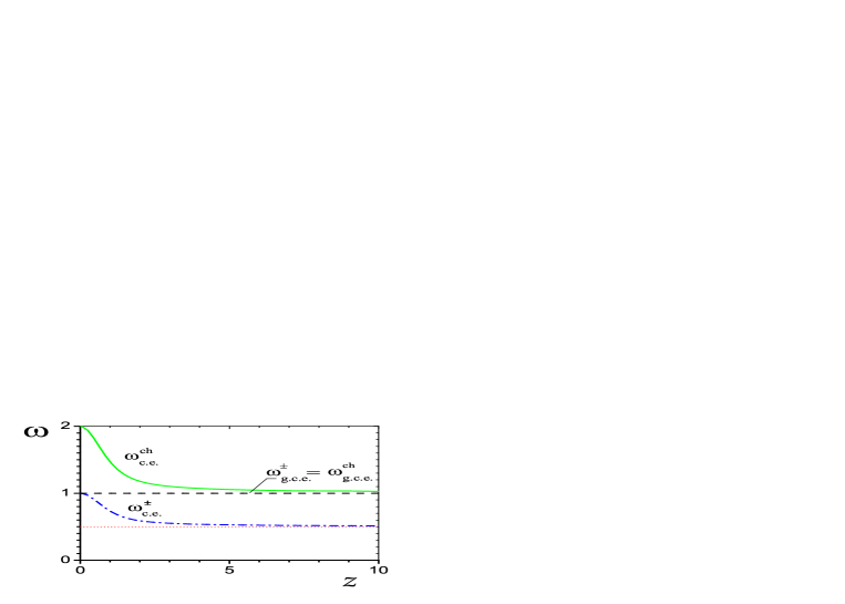
Figure 5: The scaled variances $\omega^{ch}_{c.e.}$  (28),   $\omega^{\pm}_{c.e.}$  (16)   and $\omega^{\pm}_{g.c.e.}=\omega^{ch}_{g.c.e.}=1$  (15,25) as functions of $z$.

From Eqs. (16) and (28) and the recurrence relation $I_{0}(2z)=I_{2}(2z)+I_{1}(2z)/z$ [7] it follows that $\omega_{c.e.}^{ch}=2\omega_{c.e.}^{\pm}$, i.e. the relative variance of total charge multiplicity $N_{ch}$ is two times larger than the one of $N_{\pm}$. This is because $N_{ch}=2N_{+}=2N_{-}$ in each microscopic state allowed by an exact charge conservation. One obtains a similar result for the case of particle production via decay of neutral resonances, e.g., $\rho^{0}\rightarrow\pi^{+}+\pi^{-}$. The distributions of $\pi^{+}$ and $\pi^{-}$ coincide with the $\rho^{0}$ distribution, and consequently $\omega^{\pm}=\omega$, where $\omega$ is the scaled variance of the distribution of $\rho^{0}$. But because $N_{ch}=2N_{\rho}$ one gets $\omega^{ch}=2\omega$.

Probability distribution of $\;N_{ch}\;$ in the $~{}c.e.~{}$ reads:

$$P_{c.e.}(N_{ch}) \;\equiv\;\sum_{N_{+}}^{\infty}\sum_{N_{-}=0}^{\infty}P_{c.e.}\left(N_{+},N_{-}\right)\cdot\delta\left[N_{ch}-\left(N_{+}+N_{-}\right)\right]$$ (29)

$$~{}=~{}\frac{1}{I_{0}(2z)}~{}\sum_{N_{+}=0}^{\infty}\sum_{N_{-}=0}^{\infty}\frac{z^{N_{+}}}{N_{+}!}\frac{z^{N_{-}}}{N_{-}!}\cdot\delta\left(N_{+}-N_{-}\right)\cdot\delta\left[N_{ch}-\left(N_{+}+N_{-}\right)\right]$$

$$\;=\;\frac{1}{I_{0}(2z)}~{}\left[\frac{z^{N_{ch}/2}}{(N_{ch}/2)!\;}\right]^{2}\;.$$

It coincides, of course, with $P_{c.e.}(N_{+})$ (20) at $N_{+}=N_{ch}/2$. As an example , the probability distributions $P_{g.c.e.}(N_{ch})$ (26) and $P_{c.e.}(N_{ch})$ (29) are shown for $z=0.5$ (the small system) and for $z=10$ (the large system) in Figs. 6 and 7, respectively. Only even multiplicities $N_{ch}=0,\;2,\;4\ldots\;$ are allowed in the $~{}c.e.~{}$ because of an exact charge conservation. For the small system ($z\ll 1$) the $\omega^{ch}$ reads (both $P_{g.c.e.}(N_{ch}=1)\ll 1$ and $P_{c.e.}(N_{ch}=2)\ll 1$ at $z\ll 1$):

$$\omega^{ch}_{g.c.e.} ~{}\cong~{}\frac{P_{g.c.e.}(1)\cdot 1^{2}~{}-~{}\left[P_{g.c.e.}(1)\cdot 1\right]^{2}}{P_{g.c.e.}(1)\cdot 1}~{}\cong~{}1~{},$$ (30)

$$\omega^{ch}_{c.e.} ~{}\cong~{}\frac{P_{c.e.}(2)\cdot 2^{2}\;-\;\left[P_{c.e.}(2)\cdot 2\right]^{2}\;-\;\left[P_{c.e.}(2)\cdot 2\right]^{2}}{P_{c.e.}(2)\cdot 2}~{}\cong~{}2~{}.$$ (31)

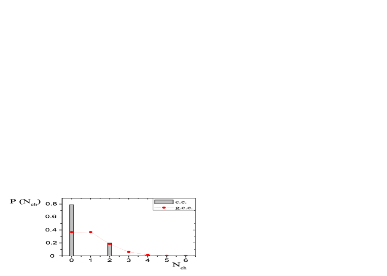
Figure 6: Multiplicity distributions of $\;N_{ch}\;$ for $\;z=0.5\;$ in the $\;g.c.e.\;$ and $\;c.e.\;$.

Figure 7: Multiplicity distributions of $\;N_{ch}\;$ for $\;z=10\;$ in the $\;g.c.e.\;$ and $\;c.e.\;$.

In the large $z$ limit the average number of charge particles $\langle N_{ch}\rangle$ and its scaled variance $\omega^{ch}$ in the $\;g.c.e.\;$, Eqs. (22) and (25), are equal to those in the $\;c.e.\;$, Eqs. (23) and (28). Nevertheless the corresponding probability distributions are different, see Fig. 7. This is because all odd multiplicities are excluded in $c.e.$ as a consequence of the charge conservation. The relation between $P_{g.c.e.}(N_{ch})$ (26) and $P_{c.e.}(N_{ch})$ (29) for the large system ($z\gg 1$) can be established as follows. Let us introduce the probability distribution $P^{*}(N_{ch})$ defined as

$$P^{*}(N_{ch})~{} \equiv~{}C\cdot P_{g.c.e.}(N_{ch})~{}, ~{}~{}N_{ch} \;=\;0,\;2,\;4,\ldots~{},$$ (32)

$$P^{*}(N_{ch})~{} \equiv~{}0~{}, ~{}~{}N_{ch} \;=\;1,\;3,\;5,\ldots~{},$$ (33)

where the constant $C$ is given by a normalization condition

$$1 ~{}=~{}\sum_{N_{ch}=0,2,4,\ldots}~{}P^{*}(N_{ch})~{}\equiv~{}C\cdot\sum_{N_{ch}=0,2,4,\ldots}~{}P_{g.c.e.}(N_{ch})$$ (34)

$$~{}=~{}C\cdot\exp(-2z)~{}\sum_{n=0}^{\infty}\frac{(2z)^{2n}}{(2n)!}~{}=~{}C\cdot\exp(-2z)~{}\cosh(2z)~{}.$$

Using Eq. (34) one gets $C=2\cdot[1+\exp(-4z)]^{-1}\cong 2$ for $z\gg 1$. The origin of the result $C\cong 2$ is the fact that

$$P_{g.c.e.}(N_{ch}+1)~{}\equiv~{}P_{g.c.e.}(N_{ch})\cdot\frac{2z}{N_{ch}+1}\cong P_{g.c.e.}(N_{ch})~{},$$ (35)

for $N_{ch}$ close to its average value $\langle N_{ch}\rangle_{g.c.e.}=2z\gg 1$, i.e. if the odd numbers $N_{ch}=1,3,5,\ldots~{}$ are forbidden the probabilities $P_{g.c.e.}(N_{ch})$ for the even numbers $N_{ch}=0,2,4,\ldots~{}$ should be approximately doubled to have a correct normalization for $P^{*}(N_{ch})$ (32).

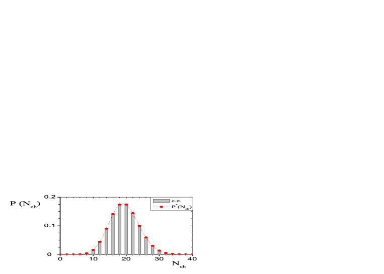
Figure 8: Multiplicity distributions $P_{c.e.}(N_{ch})$ (29) and $P^{*}(N_{ch})$ (32) for $z=10$.

Using the Stirling formula, $n!\cong n^{n}e^{-n}\sqrt{2\pi n}$, valid for $n\gg 1$, one finds that $P_{c.e.}(N_{ch})\cong P^{*}(N_{ch})$ for $N_{ch}$ close to its average value equal to $2z\gg 1$. Both distributions are plotted in Fig. 8 for a comparison.

7. Limited kinematical acceptance.   In the experimental study of nuclear collisions at high energies only a fraction of all produced particles which carry conserved charges is registered. Thus the multiplicity distribution of the measured particles is expected to be different from the distribution of all produced particles. Within $c.e.$ the effect of the limited kinematical acceptance (the acceptance in the momentum space) can be taken into account introducing a probability $q$ that a single particle is registered. Because in $c.e.$ particles are uncorrelated in momentum space the multiplicity distribution of accepted particles for a fixed number of produced particles $N$ is given by the binomial distribution:

$$P_{acc}(n,N)~{}=~{}q^{n}(1-q)^{N-n}~{}\cdot\frac{N!}{n!(N-n)!}~{}.$$ (36)

Consequently one gets:

$$\overline{n}~{}=~{}q~{}N~{},~{}~{}~{}~{}~{}\overline{n^{2}}~{}-\overline{n}^{2}~{}=~{}q(1-q)~{}N~{},$$ (37)

where $(k=1,2)$

$$\overline{n^{k}}~{}\equiv~{}\sum_{n=0}^{N}n^{k}~{}P_{acc}(n,N)~{}.$$ (38)

Introducing the probability distribution $P(N)$ the first two moments of the distribution of accepted particles can be calculated:

$$\langle n\rangle_{acc} ~{}\equiv~{}\sum_{N=0}^{\infty}P(N)~{}\sum_{n=0}^{N}n~{}P_{acc}(n_{+},N)~{}=~{}q\cdot\langle N\rangle~{},$$ (39)

$$\langle n^{2}\rangle_{acc} ~{}\equiv~{}\sum_{N=0}^{\infty}P(N)~{}\sum_{n=0}^{N}n^{2}~{}P_{acc}(n,N)~{}=~{}q^{2}\cdot\langle N^{2}\rangle~{}+~{}q(1-q)\cdot\langle N\rangle~{},$$ (40)

where ($k=1,2$)

$$\langle N^{k}\rangle~{}\equiv~{}\sum_{N=0}^{\infty}N^{k}~{}P(N)~{}.$$ (41)

Finally, the scaled variance for the accepted particles can be obtained:

$$\omega_{acc}~{}=~{}q\cdot\omega~{}+~{}(1-q)~{},$$ (42)

where $\omega$ in Eq. (42) is the scaled variance of the $P(N)$ distribution. Assuming that $P(N)$ corresponds to the $~{}c.e.~{}$, one finds from Eq. (42) the scaled variance for the accepted particles in the $~{}c.e.~{}$ $\omega_{acc}^{+}\cong 1$ for $q\ll 1$ and $\omega_{acc}^{+}\cong\omega_{c.e.}^{+}$ for $q\cong 1$.

These limiting behaviour agrees with the expectations. In the large acceptance limit ($q\approx 1$) the distribution of measured particles approaches the distribution in the full acceptance. For a very small acceptance ($q\approx 0$) the measured distribution approaches the Poisson one independent of the shape of the distribution in the full acceptance.

8. Summary.    The particle number fluctuations have been considered within canonical ensemble for a system with zero net charge. The results are compared to those in the grand canonical ensemble where only the mean value of charge is required to be zero. In the large volume limit the fluctuations in $c.e.$ are found to be different from those in the $g.c.e.$ . Thus the well known equivalence of both ensembles for the mean quantities is not valid for the fluctuations. The scaled variance of the multiplicity distribution of same charge particles is calculated to be 0.5 in the $c.e.$ and it is two times smaller than the scaled variance in $g.c.e$ . These results may be relevant for the analysis of fluctuations in high energy nuclear collisions. In view of this the influence of the limited kinematical acceptance on multiplicity fluctuations also have been discussed.

In this work the influence of the electric charge conservation was discussed. However, other material conservation laws, e.g. baryon number, strangeness or charm, can be treated within the same scheme. An extension of this work for a non-zero value of the conserved charge and several species of charged particles as well as an influence of an exact charge conservation on the energy fluctuations in the $~{}c.e.~{}$ will be presented elsewhere.

Acknowledgments.  We are grateful to A.I. Bugrij, A.P. Kostyuk, I.N. Mishustin, L.M. Satarov and Yu.M. Sinyukov for critical comments and useful discussions. We thank Marysia Gazdzicka for help in preparing the manuscript. Partial support by Institut für Theoretische Physik, Frankfurt Universität and Frankfurt Institute for Advanced Studies (M.I.G.), by DAAD scholarship under Leonard-Euler-Stipendienprogramm (O.S.Z.) and by Polish Committee of Scientific Research under grant 2P03B04123 (M.G.) is acknowledged.

Appendix.   A variable $F_{2}^{X}~{}=~{}\langle X(X-1)\rangle/\langle X\rangle^{2}$ , was used for study of the fluctuations of $N_{\pm}$ and $N_{ch}$ in small systems ($z\ll 1$) [8]. In the $~{}g.c.e.~{}$ (i.e. for the Poisson distribution of $N_{\pm}$ and $N_{ch}$) one gets $\left(F_{2}^{\pm}\right)_{g.c.e.}=\left(F_{2}^{ch}\right)_{g.c.e.}=1$, whereas in the $~{}c.e.~{}$ one finds (see also Fig. (9)):

$$\left(F_{2}^{\pm}\right)_{c.e.} ~{}\equiv~{}\frac{\langle N_{\pm}~{}\left(N_{\pm}-1\right)\rangle_{c.e.}}{\langle N_{\pm}\rangle^{2}_{c.e.}}~{}=~{}\frac{I_{0}(2z)\cdot I_{2}(2z)}{I_{1}^{2}(2z)}~{}~{}\raisebox{-2.15277pt}{$\stackrel{{\scriptstyle\cong}}{{\scriptstyle z\ll 1}}$}~{}~{}\frac{1}{2}~{}+~{}\frac{z^{2}}{6}~{},$$ (43)

$$\left(F_{2}^{ch}\right)_{c.e.} ~{}\equiv~{}\frac{\langle N_{ch}~{}\left(N_{ch}-1\right)\rangle_{c.e.}}{\langle N_{ch}\rangle^{2}_{c.e.}}~{}=~{}\frac{I_{0}^{2}(2z)~{}+~{}I_{0}(2z)\cdot I_{2}(2z)}{2~{}I_{1}^{2}(2z)}~{}~{}\raisebox{-2.15277pt}{$\stackrel{{\scriptstyle\cong}}{{\scriptstyle z\ll 1}}$}~{}~{}\frac{1}{2z^{2}}~{}.$$ (44)

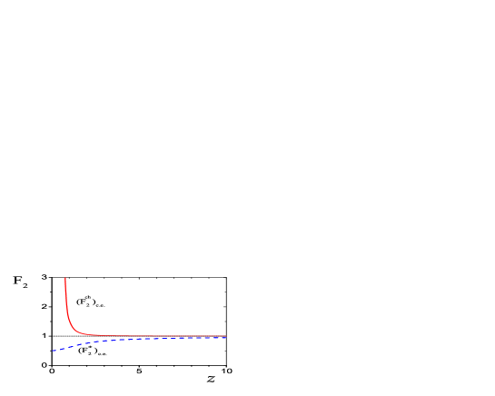
Figure 9: The fluctuation measure $F_{2}$ as a function of $z$ in the $~{}c.e.~{}$. The dashed and solid lines indicate $\left(F_{2}^{\pm}\right)_{c.e.}$ (43) and $\left(F_{2}^{ch}\right)_{c.e.}$ (44), respectively.

.

In the large volume limit $F_{2}^{\pm}\rightarrow 1$ and $F_{2}^{ch}\rightarrow 1$ because $\langle N_{\pm}\rangle^{2}\gg\langle N_{\pm}\rangle\gg 1$ (the same for $N_{ch}$). Therefore, this measure is not suitable for a study of the particle number fluctuations in the large systems.

References

[1]
P. Braun-Munzinger, K. Redlich, J. Stachel, nucl-th/0304013.
[2]
K. Werener, J. Aichelin, Phys. Rev. C 52 (1995) 1584; F. Liu,
K. Werner, J. Aichelin, Phys. Rev. C 68 (2003) 024905; F. Becattini,
L. Ferroni, hep-ph/0307061;
F. Liu, K. Werner, J. Aichelin, M. Bleicher, H. Stöcker, J. Phys. G 30 (2004) S589.
[3]
K. Redlich, L. Turko, Z. Phys. C 5 (1980) 541; J. Rafelski, M.
Danos, Phys. Lett. B 97 (1980) 279. J. Cleymans, K Redlich, E
Suhonen, Z. Phys. C 51 (1991) 137; J. Cleymans, A. Keränen, M.
Marais, E. Suhonen, Phys. Rev C 56 (1997) 2747;
F. Becattini, Z. Phys. C 69 (1996) 485; F. Becattini, U. Heinz, Z.
Phys. C 76 (1997) 269;
J. Cleymans, H. Oeschler, K. Redlich, Phys. Rev. C 59 (1999) 1663;
Phys. Lett. B 485 (2001) 27;
M.I. Gorenstein, M. Gaździcki, W. Greiner, Phys. Lett. B 483
(2000) 60;
M.I. Gorenstein, A.P. Kostyuk, H. Stöcker, W. Greiner,
Phys. Lett. B 509 (2001) 277.
[4]
J. Cleymans, H. Satz, Z. Phys. C 57 (1993) 135; J. Sollfrank, M.
Gaździcki, U. Heinz, J. Rafelski, Z. Phys. C 61 (1994) 659; G.D.
Yen, M.I. Gorenstein, W. Greiner, S.N. Yang, Phys. Rev. C56
(1997) 2210; F. Becattini, M. Gaździcki, J. Solfrank, Eur. Phys. J C 5 (1998) 143;
G.D. Yen, M.I. Gorenstein, Phys. Rev. C 59 (1999) 2788; P.
Braun-Munzinger, I. Heppe, J. Stachel, Phys. Lett.B 465 (1999) 15;
P. Braun-Munzinger, D. Magestro, K. Redlich, J. Stachel, Phys. Lett. B 518 (2001) 41; F. Becattini, M. Gaździcki, A. Keranen, J. Mannienen,
R. Stock, Phys. Rev. C 69 (2004) 024905.
[5] Misha A. Stephanov, K Rajagopal, Edward V. Shuryak,
Phys. Rev. Lett. 81 (1998) 4816; Phys. Rev. D 60 (1999)
114028;
Henning Heiselberg, Phys. Rep. 351 (2001) 161;
S. Jeon, V. Koch, arXiv:hep-ph/0304012;
M. Gaździcki, M.I. Gorenstein, St. Mrówczyński,
Phys. Lett. B 585 (2004) 115;
M.I. Gorenstein, M. Gaździcki, O.S. Zozulya, Phys. Lett.
B 585 (2004) 237.
[6]
M. Gaździcki, for the NA49 Collaboration, nucl-ex/04030023 (Talk
presented at QM’04).
[7]
M. Abramowitz and I.E. Stegun,
Handbook of Mathematical Functions, 1964 (New York: Dover).
[8]
S. Jeon, V. Koch, K. Redlich, X.N. Wang, Nucl. Phys. A 697 (2002)
546.