Traces of Thermalization at RHIC

Abstract

I argue that measurements of Au+Au collisions at 20, 130 and 200 GeV of the centrality dependence of the mean $p_{t}$ together with $p_{t}$ and net-charge fluctuations reflect the approach to local thermal equilibrium.

1 Introduction

Fluctuations of the net transverse momentum reported by the CERES, NA49, PHENIX and STAR experiments exhibit substantial dynamic contributions [1]. In particular, preliminary STAR data for Au+Au collisions at 20, 130 and 200 GeV energies show that $p_{t}$ fluctuations increase as centrality increases [2]. However, data from PHENIX and STAR exhibit a similar increase in the mean transverse momentum $\langle p_{t}\rangle$, a quantity unaffected by fluctuations [3, 4]. In [5] I ask whether the approach to local thermal equilibrium can explain the similar centrality dependence of $\langle p_{t}\rangle$ and $p_{t}$ fluctuations. Here I address new data from STAR and PHENIX, including a new and, perhaps, related effect in the centrality dependence of net-charge fluctuations [2].

Dynamic fluctuations are generally determined from the measured fluctuations by subtracting the statistical value expected, e.g., in equilibrium [6]. For particles of momenta $\mathbf{p}_{1}$ and $\mathbf{p}_{2}$, dynamic multiplicity fluctuations are characterized by

$$R_{AA}={{\langle N^{2}\rangle-\langle N\rangle^{2}-\langle N\rangle}\over{\langle N\rangle^{2}}}={{1}\over{\langle N\rangle^{2}}}\int\!d\mathbf{p}_{1}d\mathbf{p}_{2}\,r(\mathbf{p}_{1},\mathbf{p}_{2}),$$ (1)

where $\langle\cdots\rangle$ is the event average. This quantity depends only on the two-body correlation function $r(\mathbf{p}_{1},\mathbf{p}_{2})=N(\mathbf{p}_{1},\mathbf{p}_{2})-N(\mathbf{p}_{1})N(\mathbf{p}_{2})$. It is obtained from the multiplicity variance by subtracting its Poisson value $\langle N\rangle$, and divided by $\langle N\rangle^{2}$ to minimized the effect of experimental efficiency [6]. For dynamic $p_{t}$ fluctuations one similarly finds

$$\langle\delta p_{t1}\delta p_{t2}\rangle=\int\!d\mathbf{p}_{1}d\mathbf{p}_{2}\,{{r(\mathbf{p}_{1},\mathbf{p}_{2})}\over{\langle N(N-1)\rangle}}\delta p_{t1}\delta p_{t2},$$ (2)

where $\delta p_{ti}=p_{ti}-\langle p_{t}\rangle$; STAR measures this observable. The observable measured by PHENIX satisfies $F_{p_{t}}\approx N\langle\delta p_{t1}\delta p_{t2}\rangle/2\sigma^{2}$ when dynamic fluctuations are small compared to statistical fluctuations $\sigma^{2}=\langle p_{t}^{2}\rangle-\langle p_{t}\rangle^{2}$.

2 Thermalization

Thermalization occurs as scattering drives the phase space distribution within a small fluid cell toward a Boltzmann distribution that varies in space through the temperature $T(\mathbf{x},t)$. The time scale for this process is the relaxation time $\nu^{-1}$. In contrast, density differences between fluid cells must be dispersed by transport from cell to cell. The time needed for diffusion to disperse a dense fluid “clump” of size $L\sim(|\nabla n|/n)^{-1}$ is $t_{\rm d}\sim\nu L^{2}/v_{\rm th}^{2}$, where $v_{\rm th}\sim 1$ is the thermal speed of particles. This time can be much larger than $\nu^{-1}$ for a sufficiently large clumps. Global equilibrium, in which the system is uniform, can be only obtained for $t\gg t_{\rm d}$. However, the rapid expansion of the collision system prevents inhomogeneity from being dispersed prior to freeze out.

Dynamic fluctuations depend on the number of independent particle “sources.” This number changes as the system evolves. Initially, these sources are the independent strings formed as the nuclei collide. The system is highly correlated along the string, but is initially uncorrelated in the transverse plane. As local equilibration proceeds, the clumps become the sources. The fluctuations at this stage depend on number of clumps as determined by the clump size, i.e., the correlation length in the fluid. Dynamic fluctuations would eventually vanish if the system reaches global equilibrium, where statistical fluctuations are determined by the total number of particles.

3 Mean $p_{t}$ and its Fluctuations

In [5] I use the Boltzmann transport equation to show that thermalization alters the average transverse momentum following

$$\langle p_{t}\rangle=\langle p_{t}\rangle_{o}S+\langle p_{t}\rangle_{e}(1-S),$$ (3)

where $S\equiv e^{-{\mathcal{N}}}$ is the probability that a particle escapes the collision volume without scattering. The initial value $\langle p_{t}\rangle_{o}$ is determined by the particle production mechanism. If the number of collisions $\mathcal{N}$ is small, $S\approx 1-\mathcal{N}$ implies the random-walk-like increase of $\langle p_{t}\rangle$ relative to $\langle p_{t}\rangle_{o}$. For a longer-lived system, energy conservation limits $\langle p_{t}\rangle$ to a local equilibrium value $\langle p_{t}\rangle_{e}$ fixed by the temperature.

As centrality is increased, the system lifetime increases, eventually to a point where local equilibrium is reached. Correspondingly, the survival probability $S$ in (3) decreases with increasing centrality. The average $p_{t}$ peaks for impact parameters near the point where equilibrium is established. The behavior in events at centralities beyond that point depends on how the subsequent hydrodynamic evolution changes $\langle p_{t}\rangle_{e}$ as the lifetime increases. Systems formed in the most central collisions can experience a cooling that reduces (3) with proper time $\tau$ as $\langle p_{t}\rangle_{e}\propto\tau^{-\gamma}$ [5].

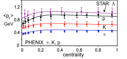
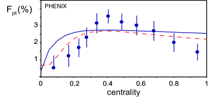
Figure 1: Mean $p_{t}$ (left) and dynamic $p_{t}$ fluctuations (right) with data [1, 3, 4]. The dashed curve in the right figure is a fit to the PHENIX data alone, while the solid curve is a fit to the STAR data. Centrality is determined by the number of participants relative to the b=0 value.

Thermalization can explain the behavior in fig. 1. The survival probability is $S=\exp\{-\int_{\tau_{0}}^{\tau_{F}}\nu(\tau)d\tau\}\approx(\tau_{0}/\tau_{F})^{\alpha}$, where $\nu=\langle\sigma v_{\rm rel}\rangle n(\tau)$ for $\sigma$ the scattering cross section, $v_{\rm rel}$ the relative velocity, and $\tau_{0,F}$ the formation and freeze out times. Longitudinal expansion implies $n(\tau)\propto\tau^{-1}$, yielding the power law with $\alpha=\nu_{0}\tau_{0}$. To fit the measured centrality dependence, I assume $\alpha=4$ and $\gamma=0.15$ in central collisions, and parameterize $S(N_{\rm part})$ by taking $\alpha\propto N_{\rm part}^{1/2}$ and $\tau_{F}-\tau_{0}\propto N_{\rm part}$, where $N_{\rm part}$ is the number of participants. I take the same $\alpha$ for all species, as appropriate for parton scattering.

Dynamic fluctuations depend on two-body correlations and, correspondingly, are quadratic in the survival probability. In [5] I add Langevin noise terms to the Boltzmann equation to describe the fluctuations of the phase space distribution. A simple limit is obtained when the initial correlations are independent of those near local equilibrium, $\langle\delta p_{t1}\delta p_{t2}\rangle=\langle\delta p_{t1}\delta p_{t2}\rangle_{o}S^{2}+\langle\delta p_{t1}\delta p_{t2}\rangle_{e}(1-S)^{2}$; this form was used in [5]. Alternatively, if the initial correlations are not far from the local equilibrium value, I find

$$\langle\delta p_{t1}\delta p_{t2}\rangle=\langle\delta p_{t1}\delta p_{t2}\rangle_{o}S^{2}+\langle\delta p_{t1}\delta p_{t2}\rangle_{e}(1-S^{2}).$$ (4)

Here I use (4), which provides somewhat better agreement with the latest STAR data in the peripheral region where thermalization is incomplete and my model assumptions most applicable. As before, the initial quantity $\langle\delta p_{t1}\delta p_{t2}\rangle_{o}$ is determined by the particle production mechanism, while $\langle\delta p_{t1}\delta p_{t2}\rangle_{e}$ describes the system near local equilibrium.

To estimate $\langle\delta p_{t1}\delta p_{t2}\rangle_{o}$ for nuclear collisions, I apply the wounded nucleon model to describe the soft production that dominates $\langle p_{t}\rangle$ and $\langle\delta p_{t1}\delta p_{t2}\rangle$, to find

$$\langle\delta p_{t1}\delta p_{t2}\rangle_{o}={{2\langle\delta p_{t1}\delta p_{t2}\rangle_{pp}}\over{N_{\rm part}}}\left({{1+R_{pp}}\over{1+R_{AA}}}\right)$$ (5)

[5]. The pre-factor is expected because (2) measures relative fluctuations and, therefore, should scale as $N_{\rm part}^{-1}$. The term in parentheses accounts for the normalization of (2) to $\langle N(N-1)\rangle$; $R_{AA}$ scales as $N_{\rm part}^{-1}$ [6]. ISR measurements imply $\langle\delta p_{t1}\delta p_{t2}\rangle_{pp}/\langle p_{t}\rangle_{pp}^{2}\approx 0.015$. I use HIJING to estimate $R_{pp}$ and $R_{AA}$, thus building in resonance and jet fluctuations.

Near local equilibrium, spatial correlations occur because the fluid is inhomogeneous – it is more likely to find particles near a dense clump. These spatial correlations fully determine the momentum correlations since the distribution at each point is thermal. The mean $p_{t}$ at each point is proportional to the temperature $T(\mathbf{x})$, so that $\langle\delta p_{t1}\delta p_{t2}\rangle_{e}\sim\int r(\mathbf{x}_{1},\mathbf{x}_{2}){\delta T}(\mathbf{x}_{1}){\delta T}(\mathbf{x}_{2})$, where $r(\mathbf{x}_{1},\mathbf{x}_{2})$ is the spatial correlation function, $\delta T=T-\overline{T}$, and $\overline{T}$ is a density-weighted average. I take $n$ ($\propto T^{3}$) and $r$ to be Gaussian with the transverse widths $R_{t}$ and $\xi_{t}$, respectively the system radius and correlation length. In [5] I obtain

$$\langle\delta p_{t1}\delta p_{t2}\rangle_{e}=F{{\langle p_{t}\rangle^{2}R_{AA}}\over{1+R_{AA}}}$$ (6)

where $R_{AA}$ is given by (1) [5]. The dimensionless quantity $F$ depends on $\xi_{t}/R_{t}$. I compute $F$ assuming $R_{t}\propto N_{\rm part}^{1/2}$; $F=0.046$ for $\xi_{t}/R_{t}=1/6$. I again use HIJING to estimate $R_{AA}$.

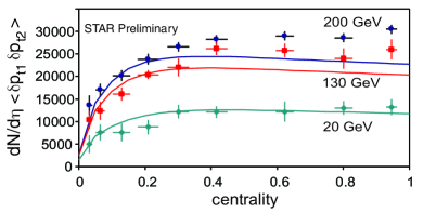
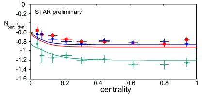
Figure 2: Dynamic $p_{t}$ (left) and net-charge fluctuations (right) with STAR data [2]. The curves and data are for three different beam energies, 20 GeV, 130 GeV and 200 GeV. Centrality is determined by the number of participants relative to the b=0 value.

Calculations in figs. 1 and 2 illustrate the common effect of thermalization on one-body and two-body $p_{t}$ observables. The solid curves in all figures are fit to STAR fluctuation data and $\langle p_{t}\rangle$ data, while the dashed curve shows a fit to the PHENIX data alone. New to this work are the STAR $p_{t}$ and net charge fluctuation data in fig. 2. To compute the energy dependence of fluctuations, I take $\alpha\propto N$ and $R_{AA}\propto N^{-1}$ for the measured multiplicity $N$. Deviations in the most central collisions at the highest beam energies may result from radial flow or, perhaps, jets [1]. Nevertheless, I stress that jets – and quenching effects – are incorporated in my calculations via the HIJING $R_{AA}$ in (6). HIJING without rescattering does not describe this data.

Net charge fluctuations in fig. 2 are characterized by $\nu_{dyn}=R^{++}+R^{--}-2R^{+-}$ for $R^{ab}$ given by (1) [6]. I therefore expect $\nu_{dyn}$ to satisfy $\nu_{dyn}=\nu_{o}S^{2}+\nu_{e}(1-S^{2})$. I use STAR pp data to fix $\nu_{0}$ and, following [6], compute $\nu_{e}/\nu_{0}$ assuming a longitudinal narrowing of the correlation length seen in balance function data [1]. The agreement of in-progress calculations with preliminary data [2] is encouraging.

References

References

- [1] J. Mitchell [PHENIX] in these proceedings.
- [2] G. Westfall [STAR] ibid.; C. Pruneau [STAR], nucl-ex/0401016.
- [3] J. Adams et al. [STAR Collab.], nucl-ex/0403020.
- [4] S. S. Adler [PHENIX Collab.], nucl-ex/0307022.
- [5] S. Gavin, Phys. Rev. Lett. to be published (2004) [nucl-th/0308067].
- [6] C. Pruneau, S. Gavin and S. Voloshin, Phys. Rev. C 66, 044904 (2002) [nucl-ex/0204011].