Effective Interactions for the Three-Body Problem

Abstract

The three-body energy-dependent effective interaction given by the Bloch-Horowitz (BH) equation is evaluated for various shell-model oscillator spaces. The results are applied to the test case of the three-body problem (³H and ³He), where it is shown that the interaction reproduces the exact binding energy, regardless of the parameterization (number of oscillator quanta or value of the oscillator parameter $b$) of the low-energy included space. We demonstrate a non-perturbative technique for summing the excluded-space three-body ladder diagrams, but also show that accurate results can be obtained perturbatively by iterating the two-body ladders. We examine the evolution of the effective two-body and induced three-body terms as $b$ and the size of the included space $\Lambda$ are varied, including the case of a single included shell, $\Lambda\hbar\omega=0\hbar\omega$. For typical ranges of $b$, the induced effective three-body interaction, essential for giving the exact three-body binding, is found to contribute $\sim$10% to the binding energy.

I Introduction

Techniques in popular use in the nuclear three-body problem include the FaddeevFaddeev (1961), Green’s Function Monte Carlo (GFMC), and correlated hyper-spherical harmonics expansion methods (see, for instance, refs.Carlson and Schiavilla (1998); Pudliner et al. (1997); Kievsky et al. (1994)). These methods have been used with realistic phenomenological potentials (e.g. Av18Wiringa et al. (1995),, CD-BonnMachleidt et al. (1996), etc. . .) with strong short-range interactions, yielding binding energies accurate to within $0.1$%Nogga et al. (2003).

All of these methods treat the bare $NN$ interactions in Hilbert spaces that are effectively infinite. Because the complexity of the Hilbert spaces grows very rapidly with nucleon number A, the extension of such methods to heavier systems becomes increasingly difficult. This motivates another approach: Solving A-body problems in more tractable finite “included spaces,” while accounting for the missing physics of the “excluded space” through an effective interaction. For shell-model-inspired effective theories that define included spaces in terms of harmonic oscillator (HO) bases, the missing physics includes both high-momentum and long-wavelength interactions. The former are missing because the included space contains only low-energy oscillator shells, while the latter are connected with the finite extent of the basis states, which are overconfined in an HO potential.

Shell-model calculations often employ two-body effective interactions, but these are generally determined phenomenologically. In recent years there has been growing success in calculating these effective interactions directly from the underlying bare interaction in a precise and systematic way (e.g. refs.Navratil and Barrett (1998); Navratil et al. (2000); Haxton and Song (2000); Haxton and Luu (2002) and references within). The purpose of this paper is to extend upon this work by calculating the more complicated $H_{eff}$ that could be used in a shell-model-inspired effective theory, through three-body order in the excluded space.. The inclusion of three-body contributions is generally believed essential in building in the density dependence crucial to saturation.

The exact effective interaction for the A-body problem is an A-body operator. The calculation of this interaction is clearly as difficult as solving the original A-body problem in an infinite Hilbert space. However, there are reasons to hope that such an A-body calculation might be unnecessary. This hope depends on the plausible notion that the effective interaction might converge as an expansion in the number of nucleons interacting in the excluded space. Were such an expansion to converge at the three- or four-body cluster level, then standard three- or four-body methods could be used to treat the excluded space. These more complicated but still tractable effective interactions could then be diagonalized in the shell-model-inspired effective theories to produce accurate binding energies and wave functions.

There are a couple of arguments that such a scheme might converge. One is the success of the shell model when phenomenological two-body effective interactions are used. This suggests that a good part of the excluded-space physics is two-body. Another is the qualitative argument that short-range clustering is increasingly unlikely as the size of the nucleon cluster increases: such spacial clustering is necessary for strong, multi-particle, high-momentum interactions. Finally, we know that the Pauli principle forbids short-range s-wave interactions above A=4.

Additional support for this notion comes from recent large-basis ab initio no-core shell-model (NCSM) calculationsNavratil and Barrett (1998); Navratil et al. (2000); Navratil and Ormand (2003). These calculations use a large but finite HO Hilbert space. A Lee-Suzuki (LS) similarity transformationSuzuki and Lee (1980) coupled with a folded-diagram sumTowner (1977) is performed on the bare NN interaction to yield an energy-independent effective interaction. Early calculations utilized only the effective two-body interaction as derived from these transformations. Hence calculations in large Hilbert spaces, or included spaces, were usually needed to ensure convergence of the binding energy (i.e. the included space had to be large enough such that the contributions to the binding energy from the effective three- and higher-body terms were small). Recent calculations that now include induced three-body interactions derived from the LS procedure show significant improvement in the convergence of binding energies for the alpha particle and some $p$-shell nucleiNavratil and Barrett (1999); Navratil and Ormand (2003).

An alternative approach to calculating the induced three-body effective interaction was developed in Ref.Haxton and Song (2000) using an excitation-energy-dependent three-body interaction based on the self-consistent solution of the Bloch-Horowitz (BH) equationBloch and Horowitz (1958). This method was successfuly used to calculate the binding energy of ³He. However, both of these works to date (i.e. LS and BH procedures) involve handling the excluded-space physics in a very large but still finite Hilbert space. This approximation introduces an extra dependence to the three-body binding on the size of the excluded space. Such dependence can only be removed by a true summation over all excluded high-energy modes (i.e. excluded space of infinte size). Though this dependence is small due to the fact that results of these previous works are quite accurate (both groups examined the convergence of their results as a function of the size of the excluded space), the rate of convergence clearly depends in detail on how singular the underlying NN interaction is. Here we develop a method for calculating the effective three-body interaction that introduces no such high-momentum cutoff, but instead truly integrates over all high-energy modes. The accuracy of our results is only limited by our numerical precision. Thus it can be applied with equal confidence to any underlying NN reaction, regardless of that potential’s description of short-range physics. This interaction is used in the simplest test cases, ³He/³H, and the results are compared with those that would result from evaluating the effective interaction only at the two-body level. Our treatment is based on solving the BH equation as well, which produces a state-dependent (and thus excitation-energy-dependent) Hermitian interaction,

$$H_{eff}(E)=P\{H+H\frac{1}{E-QH}QH\}P,$$ (1)

where

$$H = \sum_{i<j}^{A}(T_{ij}+V_{ij})$$

$$= \sum_{i}^{A}T_{i}+\sum_{i<j}^{A}V_{ij}-\frac{P_{CM}^{2}}{2M_{A}}.$$

Here the intrinsic Hamiltonian $H$ is obtained by summing the relative kinetic energy and potential energy operators $T_{ij}$ and $V_{ij}$ over all nucleon pairs $i$ and $j$. The relative kinetic energy is found by subtracting the center-of-mass (CM) kinetic energy from the total kinetic energy obtained by summing $T_{i}$ over all nucleons. $M_{A}$ is the total mass of the A-body system, $Q$ is the excluded space projection operator, and $P=1-Q$ is the included-space projection operator that defines the finite, low-energy space in which a direct diagonalization will be done, once $H_{eff}$ is obtained. As $E$ is the desired eigenvalue, which is not known $a$ $priori$, the equations must be solved self-consistently. In the calculations reported here, the Av18 potential is used as the bare $NN$ interaction and no bare three-body interaction is included.

Because our application is to ³He/³H, rather than to a heavier nucleus, we will have solved the effective interaction at the A-body level. Thus we are not testing the assumption of a cluster expansion here. Instead, our focus is on the technique for solving the effective interaction, and its relation to the approximate two-body result. Using techniques familiar from Faddeev calculations, we first determine an effective two-body-like interaction, $V_{12,eff}^{(2+1)}$, from the scattering $t$-matrix. We find that the induced effective three-body interaction can be evaluated perturbatively by iterating on $V_{12,eff}^{(2+1)}$. For a certain range of oscillator parameters $b$, convergence is achieved even for very small included spaces, including the limiting $0\hbar\omega$ space.

We also develop a non-perturbative method. By rearranging the terms of the original expansion for the three-body interaction, the series can be summed exactly through numerical solution of an integral equation. This method is very accurate and efficient for any included space and any oscillator parameter.

In Section II we generalize the two-body formulation presented in Ref.Haxton and Luu (2002). Section III describes our perturbative treatment of the effective interaction, while Section IV presents the nonperturbative solution via an integral equation. The associated discussions focus on qualitative issues, with derivations reserved for the appendices. We discuss the results and the need for a simple test of the cluster assumption (by applying current results to ⁴He) in Section V.

II Preliminaries: Two-body Review

To guarantee that $H_{eff}$, like the bare $H$, is translationally invariant one can work in a complete basis of three-nucleon HO Slater determinants that includes all configurations with quanta $N\hbar\omega<\Lambda\hbar\omega$. Such a basis, in traditional independent-particle shell-model coordinates, is overcomplete, consisting of subspaces characterized by the eigenvalues of the center-of-mass Hamiltonian $H_{CM}$ that do not interact via $H_{eff}$. For $A\leq$4, it is convenient to avoid this overcompleteness by using a Jacobi basis, which reduces the $A$-body intrinsic-Hamiltonian problem to an ($A$-1)-body problem. This is the choice we make here. The Jacobi included-space ($P$) basis corresponding to the HO shell-model basis described above is thus simple, consisting of all relative-coordinate configurations with $N\hbar\omega<\Lambda\hbar\omega$. (We note that for $A>$4, the single-particle basis is the more efficient basis for many-body calculations. However, an $H_{eff}$ developed in a Jacobi basis can be easily transformed to single-particle coordinates for use in shell-model-inspired diagonalizations.)

Such included spaces for the two-nucleon system are simple to construct. For example, a $\Lambda$=2 included space consists of spatial wave functions of the form $|n=0,l=0>$, $|n=1,l=0>$, and $|n=0,l=2>$, coupled to spin and isospin wave functions to maintain antisymmetry. This requires $l+s+t$ to be odd. The corresponding construction of fully anti-symmetrized $A$-body wave functions is less trivial Moshinsky (1969). Here we use the codes described in Ref.Navratil et al. (2000) to generate these for $A$=3. In Table 1 dimensions of various $A$=3 included spaces are given as a function of $\Lambda$.

For the three-body system one can obtain accurate results by diagonalizing the bare $H$ in a Jacobi basis, provided $\Lambda$ is made sufficiently large. This was done in Ref.Haxton and Song (2000) for the Av18 potential with $\Lambda$=60, resulting in a binding energy accurate to $\sim$ 20 keV. The motivation for solving this problem for small $\Lambda$ using effective interactions is to explore techniques that might be more feasible for larger $A$, where the model-space growth analogous to Table 1 will be much steeper.

One goal of the current work is to find techniques that might make the integration over the excluded space more tractable. In our earlier work on the two-body systemHaxton and Luu (2002) we found that this integration is difficult at both long and short distances. We found it convenient in Ref.Haxton and Luu (2002) to remove the long-distance difficulties, the pathologies associated with the overbinding of the HO, at the outset. As the overbinding of the HO becomes arbitrarily large as $r$ increases, part of the tail of the wave function remains unresolved in any finite-basis treatment– though numerically the contribution of the tail becomes increasingly unimportant in direct diagonalizations as more shells are added. (This contrasts with the short-range problem, as Av18 and other modern potentials are regulated at short distance by some assumed functional form. Such potentials can be fully resolved in finite bases, provided $\Lambda$ is larger than the scale implicit in that functional form.) In Ref.Haxton and Luu (2002) the long-range behavior was handled by the following rearrangement of Eq. (1)

$$H_{eff}=P\left\{\frac{E}{E-TQ}[T_{eff}+V_{eff}]\frac{E}{E-QT}\right\}P,$$ (2)

where

$$T_{eff} = T+T\frac{-1}{E}QT,$$ (3)

$$V_{eff} = V+V\frac{1}{E-QH}QV.$$ (4)

Here $T$ and $V$ are shorthand for $\sum_{i<j}^{A}T_{ij}$ and $\sum_{i<j}^{A}V_{ij}$, respectively. Due to space restrictions Eq. 2 was stated in Ref.Haxton and Luu (2002) without derivation. Hence we show its derivation for completeness in Appendix A.

To calculate included-space matrix elements of Eq. 2, it was first convenient to define the states

$$\widetilde{|\Omega>}=\frac{E}{E-QT}P|\Omega>=\frac{E}{E-QT}|\Omega>,$$ (5)

where $|\Omega>$ is some state that resides in the included space (i.e. $|\Omega>\in P$). With this definition, matrix elements of Eq. 2 became

$$<\Omega_{f}|H_{eff}|\Omega_{i}>=\widetilde{<\Omega_{f}|}T_{eff}+V_{eff}\widetilde{|\Omega_{i}>}.$$ (6)

Our expansion of $H_{eff}$ was formed by expanding the resolvent of $V_{eff}$ (see Eq. 4) in powers of $QV$:

$$\frac{1}{E-QH}Q=\frac{1}{E-QT}Q+\frac{1}{E-QT}QV\frac{1}{E-QT}Q+\ldots$$ (7)

An iterative procedure was then used to calculate included-space matrix elements of this expansion. At each order we solved for the self-consistent energy $E$.

The rearrangement of Eq. (2) was applied to the deuteron in Ref.Haxton and Luu (2002) and led to excellent results in perturbation theory for suitably chosen oscillator parameters $b$ (only few orders of $QV$ were needed to reproduce the deuteron binding energy to within one keV). Figure 1 shows that $\frac{E}{E-QT}$ acting on the HO state $|\Omega>$ drastically changes that state’s large-$r$ behavior: The asymptotic behavior of $\widetilde{|\Omega>}$ is $e^{-\gamma r}/\gamma r$, where $\gamma=\sqrt{mE}$, $m$ being the mass of the particleLuu (2003). As this is the proper fall-off, the overconfining effects of the HO are thus repaired. The effects are important for the deuteron, which has an extended wave function because of its small binding energy. The operator $\frac{E}{E-QT}$ modifies only those HO states that reside in the last shell of the included space. For all other states within the included space, the operator is identical to unity. The “endshell-corrected” states thus control all of the proper asymptotic behavior.

The resummation of the kinetic energy operator allows one to adjust basis wave functions to absorb much of the short-range behavior of the $NN$ interaction into the included space, leaving a weak residual interaction that can be handled perturbatively. By adjusting the oscillator parameter $b$ to low values ($\sim 0.4-0.5$ fm), the residual Q-space contributions to the binding energy due to $V\frac{1}{E-QH}QV$ can be evaluated to within $\sim$ one keV in third-order perturbation theory, even for very small included spaces. This is only possible because the kinetic energy has been summed to all orders independent of $b$, thus guaranteeing that the choice of a small $b$ will not alter the wave function at large $r$.

The optimal $b$ presumably provides the best resolution of the hard core without substantially altering the ability of the basis to reconstruct the intermediate-range potential.

In the next section we will explore a similar expansion for ³H/³He. We find modifications are necessary to account for the disparate length scales that come about from the inclusion of a third particle. Before starting this discussion, we end this section by presenting compact expressions for the operators $\frac{E}{E-QT}P$ and $\frac{1}{E-QT}Q$. Such operators appear frequently in subsequent formulae.

II.1 $\frac{E}{E-QT}P$ and $\frac{1}{E-QT}Q$ operators

The operator $\frac{1}{E-QT}$ closely resembles the free particle propagator. However, due to the projection operator Q in the denominator, calculating matrix elements of $\frac{E}{E-QT}P$ requires a little ingenuity. Here we show that the excluded-space Green’s function can be expanded in terms of the much simpler full Green’s function and operators within the included space that can be inverted easily. Following Ref.Krenciglowa et al. (1976), we first consider

$$PT\frac{E}{E-QT}P=PT\{\frac{E}{E-T}P-\frac{1}{E-T}PT\frac{E}{E-QT}\}P,$$ (8)

where $Q=1-P$. Collecting terms in this “Schwinger-Dyson” form and noting that $P^{2}=P$ gives

$$P \left\{1+T\frac{1}{E-T}\right\}P\ PT\frac{E}{E-QT}P=PT\frac{E}{E-T}P,$$ (9)

$$\Rightarrow PT\frac{E}{E-QT}P=\left\{P\frac{E}{E-T}P\right\}^{-1}\ PT\frac{E}{E-T}P.$$

The last term in Eq. 9, $PT\frac{E}{E-T}P$, can be rewritten

$$PT\frac{E}{E-T}P=EP\left(P\frac{E}{E-T}P-1\right)P.$$

Plugging the above equation into Eq. 9 finally gives

$$PT\frac{E}{E-QT}P=P\left(E-\left\{P\frac{1}{E-T}P\right\}^{-1}\right)P.$$ (10)

Similarly, the “Schwinger-Dyson” form of $\frac{E}{E-QT}P$ is

$$\frac{E}{E-QT}P=\frac{E}{E-T}P-\frac{1}{E-T}\left[PT\frac{E}{E-QT}P\right].$$ (11)

Using Eq. (10) then yields

$$\frac{E}{E-QT}P=\frac{1}{E-T}\left\{P\frac{1}{E-T}P\right\}^{-1}P.$$ (12)

This expression is relatively simple to use. The free particle propagator, $\frac{1}{E-T}$, is known analytically. Indeed, its form is diagonal in momentum space. The operator $P\frac{1}{E-T}P$ represents a matrix composed of included-space overlaps of the free particle propagator. Since we work within small included spaces, inverting this matrix is not difficult. The included-space matrix elements are easy to calculate, as analytic expressions for $<\Omega_{f}|\frac{1}{E-T}|\Omega_{i}>$ for any $A$-body system exists. These expressions involve multiple sums over hypergeometric functions and gamma functions. In Appendix C we give the relevant expression for the three-body system.

To derive an analogous expression for $\frac{1}{E-QT}Q$, we first consider

$$\frac{1}{E-QT}= \frac{1}{E-T}-\frac{1}{E-QT}PT\frac{1}{E-T}$$ (13)

$$=\frac{1}{E-T}- \frac{1}{E-T}\left\{P\frac{1}{E-T}P\right\}^{-1}\frac{T}{E}\frac{1}{E-T},$$

where we have substituted Eq. 12 in the second line above. With the use of Eqs. 12 and 13, $\frac{1}{E-QT}Q$ becomes

$$\frac{1}{E-QT}Q= \frac{1}{E-QT}(1-P)$$ (14)

$$=\frac{1}{E-T}- \frac{1}{E-T}\left\{P\frac{1}{E-T}P\right\}^{-1}\frac{1}{E-T}.$$

The physical interpretation of Eq. 14 is simple: the term on the LHS represents free propagation in the excluded ($Q$) space, while the first term on the RHS (bottom line) represents free propagation in the full ($P+Q$) space and the second term subtracts off the contribution coming from included-space ($P$) propagation.

It is convenient to make the following definitions:

$$G_{0} = \frac{1}{E-T},$$ (15)

$$\Gamma_{0}^{-1} = \left\{P\frac{1}{E-T}P\right\}^{-1}.$$ (16)

With these definitions, Eqs. 12 and 14 become

$$\frac{E}{E-QT}P = G_{0}\Gamma_{0}^{-1},$$

$$\frac{1}{E-QT}Q = G_{0}-G_{0}\Gamma_{0}^{-1}G_{0}.$$

Finally, with the expressions above, we can express our perturbative expansion in a concise form,

$$H_{eff}= E-\Gamma_{0}^{-1}+\Gamma_{0}^{-1}\Gamma_{1}\Gamma_{0}^{-1}$$ (17)

$$+ \Gamma_{0}^{-1}\left\{\Gamma_{2}-\Gamma_{1}\Gamma_{0}^{-1}\Gamma_{1}\right\}\Gamma_{0}^{-1}+ \ldots,$$

where

$$\Gamma_{1}= PG_{0}VG_{0}P$$ (18)

$$\Gamma_{2}= PG_{0}VG_{0}VG_{0}P$$

$$\vdots \quad\quad\vdots$$

$$\Gamma_{n}= PG_{0}\left(VG_{0}\right)^{n}P.$$

In the expansion given by Eq. 17, $E-\Gamma_{0}^{-1}$ corresponds to $\frac{E}{E-TQ}T_{eff}\frac{E}{E-QT}$, while $\Gamma_{0}^{-1}\Gamma_{1}\Gamma_{0}^{-1}$ corresponds to $\frac{E}{E-TQ}V\frac{E}{E-QT}$, and so on. As we stressed in Ref.Haxton and Luu (2002), matrix elements of the operators shown in Eq. 18 can be simply calculated using a recursive procedure.

III A Perturbative Three-body calculation

Similarly, one might apply the expansion given by Eqs. (17) and (18) directly to ³He/³H. As was done in the two-body system, we construct endshell-corrected states to build in the correct aymptotic forms. Figure 2 shows momentum-space results for one $10\hbar\omega$ endshell state. As expected, the modified wavefunction acquires a strong peak near zero-momentum, corresponding to large-r corrections.

To determine an optimal $b$ for subsequent calculations, $H$ is minimized within the included space. The results are given in Fig. 3 for several included spaces. As expected, the endshell states improve the binding of the three-body system and lower the optimal $b$, relative to uncorrected HO results. However, the improved binding energies are still far away from the exact answers. This contrasts with the deuterium results (see Fig.2 of Ref. Haxton and Luu (2002)), where 0th-order results using endshell states were accurate ( $\sim$ 50 keV), and became nearly exact in second- or third-order perturbation theory. The 0th order A=3 results underbind by $\sim 3$ MeV.

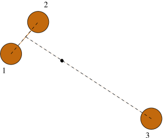
Figure 5: Problematic configuration for three-body expansion. Such a configuration consists of two closely spaced particles (1 and 2), while a third particle is separated far from the first two.

As Fig. 4 shows, these results are not corrected in perturbation theory. Successive orders produce wildly oscillating values for the binding energy, in contrast to the rapid convergence found for the deuteron. The difficulty is that a single distance scale $b$ does not provide sufficient freedom to describe short-range behavior governed by two relative cordinates. Extended states such as those of Fig. 5 are problematic. Once one makes a choice of Jacobi coordinates, the short-range behavior of some two-body cluster will be difficult to describe. For example, the choice $(\vec{r}_{3}-\vec{r}_{2})/\sqrt{2}$ and $(2\vec{r}_{1}-\vec{r}_{3}-\vec{r}_{2})/\sqrt{6}$ prevents one from adjusting $b$ to account for the short-range interactions of nucleons 1 and 2. Consequently, important hard-core interactions lie outside the included space, leading to nonperturbative behavior.

III.1 Invoking Faddeev Decompositions

Because the deuteron was easily treated, it is possible to sum to all orders the repeated excluded space scatterings of any two-nucleon cluster. Such a partial summation should account for the strong repulsive interaction between any two coupled nucleons, leaving only intermediate- and long-range interactions. Such interactions can be treated reasonably accurately within the included space using our endshell-corrected states, leaving perturbative corrections. This partial summation corresponds to the Faddeev decompositionFaddeev (1961); Glockle (1983). The starting point is again Eq. 6,

$$<\Omega_{f}|H_{eff}|\Omega{i}>=\widetilde{<\Omega_{f}|}T_{eff}+V_{eff}\widetilde{|\Omega_{i}>},$$

where we cast $V_{eff}$ in its integral form,

$$V_{eff}=V^{3}_{eff}=V+V\frac{1}{E-QT}QV^{3}_{eff}.$$ (19)

Here the superscript ³ denotes that this is a three-body effective interaction. Now consider the state $V^{3}_{eff}\widetilde{|\ \Omega_{\sigma}>}$ $\equiv$ $\widetilde{|\ \Psi_{\sigma}>}$, which satisfies

$$\widetilde{|\ \Psi_{\sigma}>}=V\widetilde{|\ \Omega_{\sigma}>}+V\frac{1}{E-QT}Q\widetilde{|\ \Psi_{\sigma}>}.$$ (20)

This can be decomposed into Faddeev components $\widetilde{|\Psi_{\sigma}>_{ij}}$, given by

$$\widetilde{|\ \Psi_{\sigma}>}_{12}= V_{12}\widetilde{|\ \Omega_{\sigma}>}+V_{12}\frac{1}{E-QT}Q\widetilde{|\ \Psi_{\sigma}>},$$ (21)

$$\widetilde{|\ \Psi_{\sigma}>}_{23}= V_{23}\widetilde{|\ \Omega_{\sigma}>}+V_{23}\frac{1}{E-QT}Q\widetilde{|\ \Psi_{\sigma}>},$$

$$\widetilde{|\ \Psi_{\sigma}>}_{31}= V_{31}\widetilde{|\ \Omega_{\sigma}>}+V_{31}\frac{1}{E-QT}Q\widetilde{|\ \Psi_{\sigma}>},$$

where

$$\widetilde{|\ \Psi_{\sigma}>}=\widetilde{|\ \Psi_{\sigma}>}_{12}+\widetilde{|\ \Psi_{\sigma}>}_{23}+\widetilde{|\ \Psi_{\sigma}>}_{31}.$$ (22)

Equations 22 and 21 show that the Faddeev components require the solution of three coupled integral equations. For example, $\widetilde{|\ \Psi_{\sigma}>}_{12}$ satisfies

$$\widetilde{|\ \Psi_{\sigma}>}_{12} =V_{12}\widetilde{|\ \Omega_{\sigma}>}+$$ (23)

$$V_{12} \frac{1}{E-QT}Q\left(\widetilde{|\ \Psi_{\sigma}>}_{12}+\widetilde{|\ \Psi_{\sigma}>}_{23}+\widetilde{|\ \Psi_{\sigma}>}_{31}\right).$$

Equation 23 can be inverted with respect to the $\widetilde{|\ \Psi_{\sigma}>}_{12}$ Faddeev component, giving

$$\widetilde{|\ \Psi_{\sigma}>}_{12} =V^{(2+1)}_{12,eff}\widetilde{|\ \Omega_{\sigma}>}+$$ (24)

$$V^{(2+1)}_{12,eff} \frac{1}{E-QT}Q\left(\widetilde{|\ \Psi_{\sigma}>}_{23}+\widetilde{|\ \Psi_{\sigma}>}_{31}\right),$$

where

$$V^{(2+1)}_{12,eff}= \frac{1}{1-V_{12}\frac{1}{E-QT}Q}V_{12}$$ (25)

$$= V_{12}+V_{12}\frac{1}{E-QT-QV_{12}}QV_{12}$$

$$= V_{12}+V_{12}\frac{1}{E-QT}QV^{(2+1)}_{12,eff}.$$

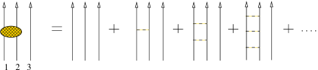
Figure 6: Diagrammatic expansion of $\frac{1}{E-QT-QV_{12}}Q.$ The dashed lines correspond to $V_{12}$ interactions.

Analogous equations can be found for the remaining Faddeev components. The superscript ⁽²⁺¹⁾ indicates that the effective interaction given by Eq. 25 represents the sum of repeated potential scatterings between the same two nucleons (in this case, nucleons 1 and 2), while the third nucleon remains a spectator, as illustrated in Fig. 6.

This expression is exactly the partial sum mentioned above. Notice that the middle expression in Eq. 25 is very similar to Eq. 4. Furthermore, the integral form of $V^{(2+1)}_{12,eff}$ is similar to that of the G-matrixBrueckner (1955). Yet there are subtleties that differentiate the two. We will return to this point later. The integral equation given by Eq. 25 can also be solved exactly in terms of the (2+1)-body $t$-matricesGlockle (1983). In Appendix B we show

$$V^{(2+1)}_{12,eff}=t_{12}-t_{12}G_{0}\left[\Gamma_{0}+\Gamma^{(2+1)}_{\infty}\right]^{-1}G_{0}t_{12},$$ (26)

where

$$t_{12} = V_{12}+V_{12}G_{0}t_{12}$$ (27)

$$\Gamma^{(2+1)}_{\infty} = PG_{0}t_{12}G_{0}P,$$ (28)

and $\Gamma_{0}$ is given by Eq. 16. The physical interpretation of Eq. 26 is similar to the one given below Eq. 13: the first term on the RHS represents the effective interaction coming from repeated scatterings in the full ($P+Q$) space, while the second term subtracts off the contribution from the included ($P$) space.

The advantage in using the Faddeev decompositions comes from exploiting particle exchange symmetries. As the states $|\ \Omega_{\sigma}>$ are fully anti-symmetric, the individual Faddeev components can be related to each other by simple permutation operatorsGlockle (1983). In particular,

$$\widetilde{|\ \Psi_{\sigma}>}_{23}= P_{12}P_{23}\widetilde{|\ \Psi_{\sigma}>}_{12},$$ (29)

$$\widetilde{|\ \Psi_{\sigma}>}_{31}= P_{12}P_{13}\widetilde{|\ \Psi_{\sigma}>}_{12},$$

$$\Rightarrow\widetilde{|\ \Psi_{\sigma}>}= (1+\Pi)\widetilde{|\ \Psi_{\sigma}>}_{12},$$

where the permutation operator $\Pi$ is defined as $\Pi=P_{12}P_{13}+P_{12}P_{23}$. The last expression in Eq. 23 then becomes

$$\widetilde{|\ \Psi_{\sigma}>}_{12}=V^{(2+1)}_{12,eff}\widetilde{|\ \Omega_{\sigma}>}+V^{(2+1)}_{12,eff}\frac{1}{E-QT}Q\Pi\widetilde{|\ \Psi_{\sigma}>}_{12},$$

which can be formally inverted with respect to $\widetilde{|\ \Psi_{\sigma}>}_{12}$ to give

$$\widetilde{|\ \Psi_{\sigma}>}_{12}=\left(V^{(2+1)}_{12,eff}+V^{(3+0)}_{12,eff}\right)\widetilde{|\ \Omega_{\sigma}>}.$$ (30)

where

$$V^{(3+0)}_{12,eff}\equiv V^{(2+1)}_{12,eff}\frac{1}{E-QT-Q\Pi V^{(2+1)}_{12,eff}}Q\Pi V^{(2+1)}_{12,eff}.$$ (31)

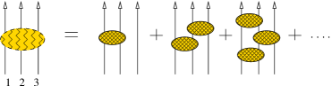
Figure 7: Diagrammatic expansion of $\frac{1}{E-QH}Q$ for the three-body problem. The shaded ovals on the RHS are given by Fig. 6. Aside from the first term on the RHS, the remaining terms contribute to $V^{(3+0)}_{12,eff}$.

Equation 31 defines the induced three-body interaction coming from repeated scatterings of $V^{(2+1)}_{12,eff}$ (see Fig. 7). The operator $\Pi$ ensures that every insertion of $V^{(2+1)}_{12,eff}$ represents scatterings coming from different pairs of nucleons (i.e. the rungs of Fig. 7 alternate), preventing any double couting. As there are no spectator nucleons in this expression, it is labeled with the superscript ⁽³⁺⁰⁾.

Matrix elements $<H_{eff}>$ are given by

$$\widetilde{<\Omega_{i}|}H_{eff}\widetilde{|\ \Omega_{f}>}=$$ (32)

$$\widetilde{<\Omega_{i}|}T_{eff}+\sum_{l<m}^{3} \left(V^{(2+1)}_{lm,eff}+V^{(3+0)}_{lm,eff}\right)\widetilde{|\ \Omega_{f}>}$$

$$=\widetilde{<\Omega_{i}|}T_{eff}+3 \left(V^{(2+1)}_{12,eff}+V^{(3+0)}_{12,eff}\right)\widetilde{|\ \Omega_{f}>},$$

where the factor of $3$ in the last expression comes from the anti-symmetry of the states. An expansion of Eq. 32 can now be found by expanding the resolvent of Eq. 31 in powers of $\Pi V^{(2+1)}_{12,eff}$,

$$\frac{1}{E-QT-Q\Pi V^{(2+1)}_{12,eff}}Q =$$

$$\frac{1}{E-QT}Q+\frac{1}{E-QT} Q\Pi V^{(2+1)}_{12,eff}\frac{1}{E-QT}Q+\ldots.$$

Expressions analogous to those of Eq. (18) can be constructed from $\Pi$ and $V^{(2+1)}_{12,eff}$,

$$\Gamma_{n}= PG_{0}\left(V^{(2+1)}_{12,eff}G_{0}\right)^{n}P$$ (33)

$$\gamma_{n}= PG_{0}\left(\Pi V^{(2+1)}_{12,eff}G_{0}\right)^{n}P$$

$$\tilde{\Gamma}_{n}= PG_{0}V^{(2+1)}_{12,eff}G_{0}\left(\Pi V^{(2+1)}_{12,eff}G_{0}\right)^{n-1}P.$$

Combining Eq. 33 with the expansion of Eq. 32 gives the final result (compare with Eq. 17),

$$H_{eff}= E-\Gamma_{0}^{-1}+3\Gamma_{0}^{-1}\Gamma_{1}\Gamma_{0}^{-1}+$$ (34)

$$3\Gamma_{0}^{-1} \left\{\tilde{\Gamma}_{2}-\Gamma_{1}\Gamma_{0}^{-1}\gamma_{1}\right\}\Gamma_{0}^{-1}+$$

$$3\Gamma_{0}^{-1} \{\tilde{\Gamma}_{3}-\tilde{\Gamma}_{2}\Gamma_{0}^{-1}\gamma_{1}-\Gamma_{1}\Gamma_{0}^{-1}\gamma_{2}+$$

$$\quad\quad\quad\quad\quad\quad\Gamma_{1}\Gamma_{0}^{-1}\gamma_{1}\Gamma_{0}^{-1}\gamma_{1}\}\Gamma_{0}^{-1}+\ldots$$

Figure 8 shows the convergence of the binding energies for ³H and ³He for several included-space and oscillator parameter choices. The expansion of Eq. (34) converges even for very small included spaces, including $\Lambda=0$ (which corresponds to a single matrix element). Surprisingly, the most rapid convergence occurs for the smallest included spaces. We do not have a convincing physical explanation for this result.

Note that the zeroth order results (i.e. $E-\Gamma_{0}^{-1}+3\Gamma_{0}^{-1}\Gamma_{1}\Gamma_{0}^{-1}$) all overbind in Fig. 8. This is possible since the zeroth order calculation is no longer variational, as $V^{(2+1)}_{12,eff}$ now depends on $E$ (see Eq. 25). Hence there is no prescribed method for finding the optimal $b$, other than by trial and error. (We stress that fully converged results will be independent of $b$, as we have executed the effective theory faithfully. By an optimal $b$ we mean one that will speed the convergence.) The values of $b$ used in Fig. 8 should be near the optimal. Note that these values are much larger than those found for the deuteron calculations of Ref.Haxton and Luu (2002). Since $V^{(2+1)}_{12,eff}$ is calculated exactly, all short range two-body correlations are correctly taken into account. Hence $b$ is no longer forced to small values by the demands of short-$r$ physics, but instead can relax to values characteristic of the size of the three-body system.

As mentioned earlier, $V^{(2+1)}_{12,eff}$ is reminiscent of the $G$-matrix found in traditional nuclear many-body theory, which is also an infinite ladder sum in particle-particle propagation. However the differences are substantial. Traditional shell-model calculations have always used G-matrix interactions at the two-body level, ignoring any dependence the operator may have on spectator nucleons (including in general certain violations of the Pauli principle). The operator $V^{(2+1)}_{12,eff}$, on the other hand, depends explicitly on the spectator nucleon kinetic energy, as well as on the kinetic energies of the interacting nucleons. This dependence is manifest in Eq. 25, as the operator $T$ in the resolvent $\frac{E}{E-QT}Q$ represents the sum of the kinetic energies of all nucleons. This dependence on the spectator nucleon is essential for calculating the correct two-body correlations within the three-body system, as $Q$ is defined by the quanta carried by the three-body configurations. Similarly, for $A$-body calculations, the analogous operator, $V^{(2+(A-2))}_{12,eff}$, would carry the dependence of all spectator nucleons.

It appears that a perturbative expansion for the binding energy of ³He/³H results only if one first sums two-body ladder interactions to all orders (i.e. $V^{(2+1)}_{12,eff}$). This summation softens the two-body interaction, which on iteration can then generate the effective three-body interaction (i.e. $V^{(3+0)}_{12,eff}$) perturbatively. A similar procedure was followed in Refs.Bedaque et al. (2000); Gabbiani et al. (2000), where the triton binding energy was calculated by perturbing in di-baryon fields. The di-baryon fields themselves represent an infinite scattering of two-body interactions, in analogy with $V^{(2+1)}_{12,eff}$.

IV A non-perturbative three-body calculation

A drawback of the perturbative approach of the previous section is that for each included space defined by $\Lambda$, there is only a limited range of $b$s for which the expansion converges readily. Furthermore, there is no definite procedure for estimating the optimal $b$, as the zeroth-order calculation is no longer variational. Thus a nonperturbative procedure would be attractive: any $b$ could be chosen, and physical observables would prove to be independent of $b$, as they must for a rigorously executed effective theory. Such a non-perturbative summation is indeed possible by reshuffling the terms of Eq. (34) to form a summable geometric series and by numerically solving an integral equation. This approach provides an opportunity to directly compare the relative sizes of $V^{(2+1)}_{12,eff}$ and $V^{(3+0)}_{12,eff}$ as functions of both $\Lambda$ and $b$.

In this section we only show results for the triton system, as ³He calculations produce similar results. The starting point this time is Eq. 34,

$$H_{eff}=E-\Gamma_{0}^{-1}+3\Gamma_{0}^{-1}\Gamma_{1}\Gamma_{0}^{-1}+$$ (35)

$$3\Gamma_{0}^{-1}\left\{\tilde{\Gamma}_{2}-\Gamma_{1}\Gamma_{0}^{-1}\gamma_{1}\right\}\Gamma_{0}^{-1}+$$

$$3\Gamma_{0}^{-1}\left\{\tilde{\Gamma}_{3}-\tilde{\Gamma}_{2}\Gamma_{0}^{-1}\gamma_{1}-\Gamma_{1}\Gamma_{0}^{-1}\gamma_{2}+\Gamma_{1}\Gamma_{0}^{-1}\gamma_{1}\Gamma_{0}^{-1}\gamma_{1}\right\}\Gamma_{0}^{-1}$$

$$+\ldots,$$

where the set $\{\Gamma_{n},\tilde{\Gamma}_{n},\gamma_{n}\}$ is given by Eq. 33. This expansion can be rearranged into

$$H_{eff} =E-\Gamma_{0}^{-1}+3\Gamma_{0}^{-1}\Gamma_{1}\Gamma_{0}^{-1}$$ (36)

$$+ 3(\Gamma_{0}^{-1}\left(\tilde{\Gamma}_{2}+\tilde{\Gamma}_{3}+\ldots\right)\Gamma_{0}^{-1}-\Gamma_{0}^{-1}\left(\tilde{\Gamma}_{2}+\tilde{\Gamma}_{3}+\ldots\right)\Gamma_{0}^{-1}\left(\gamma_{1}+\gamma_{2}+\ldots\right)\Gamma_{0}^{-1}+\ldots)$$

$$-3(\Gamma_{0}^{-1} \Gamma_{1}\Gamma_{0}^{-1}\left(\gamma_{1}+\gamma_{2}+\ldots\right)\Gamma_{0}^{-1}-\Gamma_{0}^{-1}\Gamma_{1}\Gamma_{0}^{-1}\left(\gamma_{1}+\gamma_{2}+\ldots\right)\Gamma_{0}^{-1}\left(\gamma_{1}+\gamma_{2}+\ldots\right)\Gamma_{0}^{-1}+\ldots).$$

Equation 36 can be verified by expanding its terms out and directly comparing with Eq. 35. The following definitions can be made to simplify Eq. 36,

$$\tilde{\Gamma}_{\infty} =\tilde{\Gamma}_{2}+\tilde{\Gamma}_{3}+\ldots$$ (37)

$$\gamma_{\infty} =\gamma_{1}+\gamma_{2}+\ldots,$$

where the above expressions represent infinite summations. Substituting these expressions into Eq. 36 gives

$$H_{eff}=E-\Gamma_{0}^{-1}+3\Gamma_{0}^{-1}\Gamma_{1}\Gamma_{0}^{-1}$$ (38)

$$+ 3(\Gamma_{0}^{-1}\tilde{\Gamma}_{\infty}\Gamma_{0}^{-1}-\Gamma_{0}^{-1}\tilde{\Gamma}_{\infty}\Gamma_{0}^{-1}\gamma_{\infty}\Gamma_{0}^{-1}+\ldots)$$

$$- 3(\Gamma_{0}^{-1}\Gamma_{1}\Gamma_{0}^{-1}\gamma_{\infty}\Gamma_{0}^{-1}-\Gamma_{0}^{-1}\Gamma_{1}\Gamma_{0}^{-1}\gamma_{\infty}\Gamma_{0}^{-1}\gamma_{\infty}\Gamma_{0}^{-1}+\ldots)$$

The two geometric series in the equation above can be summed to give the final desired result,

$$H_{eff}= E-\Gamma_{0}^{-1}+3\Gamma_{0}^{-1}\Gamma_{1}\Gamma_{0}^{-1}$$ (39)

$$+ 3\Gamma_{0}^{-1}\left(\tilde{\Gamma}_{\infty}-\Gamma_{1}\Gamma_{0}^{-1}\gamma_{\infty}\right)\frac{1}{1+\Gamma_{0}^{-1}\gamma_{\infty}}\Gamma_{0}^{-1}$$

$$= T_{eff}+3V^{(2+1)}_{12,eff}+3V^{(3+0)}_{12,eff},$$

where we have made the following identifications,

$$T_{eff}= E-\Gamma_{0}^{-1}$$

$$V^{(2+1)}_{12,eff}= \Gamma_{0}^{-1}\Gamma_{1}\Gamma_{0}^{-1}$$

$$V^{(3+0)}_{12,eff}= \Gamma_{0}^{-1}\left(\tilde{\Gamma}_{\infty}-\Gamma_{1}\Gamma_{0}^{-1}\gamma_{\infty}\right)\frac{1}{1+\Gamma_{0}^{-1}\gamma_{\infty}}\Gamma_{0}^{-1}.$$

The usefulness of Eq. (39) depends on having an efficient method for calculating the included-space matrix elements of $\gamma_{\infty}$ and $\tilde{\Gamma}_{\infty}$. This can be done by first considering the state $\gamma_{\infty}|\ \Omega_{\sigma}>=|\Psi_{\sigma}>$, which, using Eq. 37, satisfies

$$|\Psi_{\sigma}>= \gamma_{1}|\ \Omega_{\sigma}>+\gamma_{2}|\ \Omega_{\sigma}>+\ldots$$ (40)

$$=G_{0} \Pi V_{12}G_{0}|\ \Omega_{\sigma}>+G_{0}\Pi V_{12}G_{0}\Pi V_{12}G_{0}|\ \Omega_{\sigma}>+\ldots$$

$$=G_{0} \Pi V_{12}G_{0}|\ \Omega_{\sigma}>+G_{0}\Pi V_{12}|\Psi_{\sigma}>.$$

Hence $|\Psi_{\sigma}>$ satisfies the Fredholm integral equation of the second kindHackbusch (1995). There are numerous numerical methods available for solving this particular integral equation. We use a general projection algorithmHackbusch (1995). Due to the large number of partial waves and the complicated structure of the operator $\Pi$, solving the integral equation by matrix inversion is impractical.

Once $|\Psi_{\sigma}>$ is found, the matrix elements

$$<\Omega_{i}|\gamma_{\infty}|\ \Omega_{\sigma}>=<\Omega_{i}|\Psi_{\sigma}>$$

can be evaluated. Then the matrix elements $<\Omega_{i}|\tilde{\Gamma}_{\infty}|\Omega_{\sigma}>$ are easily calculated since

$$\tilde{\Gamma}_{\infty}|\Omega_{\sigma}>=G_{0}V_{12}|\Psi_{\sigma}>,$$

which can be verified using Eqs. 33 and 37. Hence

$$<\Omega_{i}|\tilde{\Gamma}_{\infty}|\ \Omega_{\sigma}>=<\Omega_{i}|G_{0}V_{12}|\Psi_{\sigma}>.$$

Tables 2 and 3 show the calculated binding energies for the triton system as a function of the included-space size $\Lambda$ and oscillator parameter $b$. In Table 2 we have ignored the small isospin-violating parts of the Av18 potential. Hence isospin is conserved at $T=1/2$. Table 3 includes isospin-violating contributions. This causes a small admixture of $T=3/2$ components into the ground state. At about the keV level, the results are independent of the choice of the included space, i.e., of $b$ and $\Lambda$. The $\sim$ few keV variations illustrate the level of our numerical precision. Note that for the values $b$=.83 and 1.17 fm, our calculations of the previous section would give non-converging binding energies. This of course emphasizes the non-perturbative nature of these calculations.

Note that Eq. 39 has the correct limiting behavior as $\Lambda\rightarrow\infty$, $H_{eff}\rightarrow H$. In this limit the projection operator $P\rightarrow 1$, giving $\Gamma_{0}^{-1}\rightarrow G_{0}^{-1}$. Thus

$$E-\Gamma_{0}^{-1}\overset{\Lambda\rightarrow\infty}{\longrightarrow}T.$$

It is also straightforward to show that

$$V^{(2+1)}_{12,eff}=\Gamma_{0}^{-1}\Gamma_{1}\Gamma_{0}^{-1} \overset{\Lambda\rightarrow\infty}{\longrightarrow}\frac{1}{1+t_{12}G_{0}}t_{12}$$

$$=V_{12},$$

where we have used Eq. 27 to obtain the second line above. Finally, it is obvious that $V^{(3+0)}_{12,eff}$ vanishes in this limit since

$$\tilde{\Gamma}_{\infty}-\Gamma_{1}\Gamma_{0}^{-1}\gamma_{\infty}\overset{\Lambda\rightarrow\infty}{\longrightarrow}\quad\tilde{\Gamma}_{\infty}-G_{0}V\gamma_{\infty}=0.$$

Hence $H_{eff}\rightarrow H$.

Tables 4- 6 show the variation of the matrix elements of $V^{(2+1)}_{12,eff}$ and $V^{(3+0)}_{12,eff}$ with $\Lambda$ and $b$. Isospin-violating effects have also been ignored in these results. As the number of included-space examples is small, it is difficult to extract any limiting behavior. Yet it does seem that as $\Lambda$ increases, matrix elements of $V^{(2+1)}_{12,eff}$ approach the bare $V_{12}$ (indicated by the symbol $\infty$ in the tables). This is especially evident in Table 5, where the effect of renormalization is small (i.e. the renormalized matrix elements are not too different from their bare matrix elements). In the cases involving $V^{(3+0)}_{12,eff}$, limiting behavior is also difficult to extract. Indeed, in Tables. 4 and 6 matrix elements of $V^{(3+0)}_{12,eff}$ tend to grow away from zero with increasing $\Lambda$ rather than tend toward zero. However, in these cases the renormalization is strong, so that limiting behavior would not be expected for such small $\Lambda$. In Table 5 the renormalization is much weaker, and the limiting behavior $3V^{(3+0)}_{12,eff}\rightarrow 0$ is clearly seen for the $\hbar\omega=15$ and $=60$ MeV examples. It is also clear from Tables. 4- 6 that the matrix elements of $V^{(2+1)}_{12,eff}$ and $V^{(3+0)}_{12,eff}$ have a strong dependence on $\Lambda$ and $b$ ($\hbar\omega$), a dependence often ignored in traditional shell-model calculations.

Generally the contribution of $<V^{(3+0)}_{12,eff}>$ to the overall binding energy is small compared to $<V^{(2+1)}_{12,eff}>$ ($\sim 10\%$ of $V^{(2+1)}_{12,eff}$), as is evident from Fig. 9. This graph gives the $<T_{eff}>$, $3<V^{(2+1)}_{12,eff}>$, and $3<V^{(3+0)}_{12,eff}>$ contributions to the binding energy as functions of $\Lambda$ and $b$. Interestingly, for each included-space $\Lambda$, there are two values of $b$ at which the contribution of $<V^{(3+0)}_{12,eff}>$ completely vanishes. Table 7 lists specific values. If this result proves to be a generic property of the three-body $H_{eff}$ in heavier nuclei (that is, if zeros appear in those calculations at approximately the same value of $b$), this could greatly simplify the more complicated included-space diagonalizations required in heavy systems. For example, the three-body contribution could be ignored or could be explored in low-order perturbation theory. This would require establishing that the A=3 zero for $<V^{(3+0)}_{12,eff}>$ does persist at about the same $b$ in heavier systems. This seems plausible, as the three-body ladder in a heavy nucleus is quite similar to that in A=3.

V Conclusion

We found in Section III that the simple perturbative scheme found in Ref.Haxton and Luu (2002) (i.e. Eq. (17)) did not directly extend to the three-body system due to the additional length scale introduced by the third nucleon. For any choice of Jacobi coordinates, this second length scale excludes a class of hard-core interactions from the included space regardless of the choice of $b$. This problem was circumvented by invoking the Faddeev decomposition on $H_{eff}$, which allowed us to sum to all orders the repeated potential scattering between the same two nucleons, generating $V^{(2+1)}_{12,eff}$. Hence the strong repulsive two-nucleon force was treated non-perturbatively. The remaining contribution to $H_{eff}$, $V^{(3+0)}_{12,eff}$, can then be calculated by summing repeated insertions of $V^{(2+1)}_{12,eff}$ on alternate pairs of nucleons. For certain ranges of $b$, this expansion converged after several orders of perturbation even for the smallest allowed included spaces, as shown in Fig. 8.

In Section IV we described a non-perturbative method for calculating $H_{eff}$ in the three-body system, summarized in Eq. (39). This allowed a direct comparison of the contributions of $<T_{eff}>$, $<V^{(2+1)}_{12,eff}>$, and $<V^{(3+0)}_{12,eff}>$. Because the calculation was non-perturbative, we were able to explore the dependence of the included-space matrix elements (and establish the independence of the binding energy) for a wider range of $b$s and $\Lambda$s. Also, for each included space, we found two values of $b$ where the total binding was due to $V^{(2+1)}_{12,eff}$, a result that should be explored in heavier systems. The numerical methods included an efficient algorithm for solving integral equations (i.e. Eq. (40)). In the current applications to A=3 systems, the numerical effort was not substantial.

Work is in progress to apply a similar formalism to the alpha particle. As in the three-body case, one must account for the various length scales inherent to the four-body system. This can be done by invoking the Faddeev-Yakubovsky decompositions on $H_{eff}$, in direct analogy to the three-body decompositions presented in this paper. Such a procedure will not only yield $<T_{eff}>$, $<V^{(2+2)}_{12,eff}>$ and $<V^{(3+1)}_{12,eff}>$ (direct analogs of $<V^{(2+1)}_{12,eff}>$ and $<V^{(3+0)}_{12,eff}>$), but also $<V^{(4+0)}_{12,eff}>$. This last expression represents the induced effective four-body interaction. It will be interesting to see if these calculations verify the commonly implicit assumption of the hierarchical sizes of these interactions (i.e. $V^{(2+2)}_{12,eff}\ <\ V^{(3+1)}_{12,eff}\ <\ V^{(4+0)}_{12,eff}$). The four-body effective interaction is the most complicated lowest-order (s-wave) operator that can be constructed. Furthermore, alpha-particle clustering is an important phenomenological feature of nuclear structure, apparent even in simple systems like ⁸Be. Thus it will be interesting to determine the size of this contribution. The A=4 calculations will also check whether zeros in the three-body effective interaction persist. If they do, we may learn something about their “trajectories” in $b$ as A is inceased.

Appendix A Derivation of Eq. 17

For completeness, we show the derivation of Eq. 2, which was first used in Ref.Haxton and Luu (2002) in deriving a perturbative expansion for the deuteron. We begin by explicitly expressing the BH equation in its various components,

$$H_{eff}= H+H\frac{1}{E-QH}QH$$ (41)

$$= H+T\frac{1}{E-QH}QT+V\frac{1}{E-QH}QV+T\frac{1}{E-QH}QV+V\frac{1}{E-QH}QT.$$

Next consider the operator

$$T\frac{1}{E-QH}QT= T\left[\frac{1}{E-QT}+\frac{1}{E-QT}QV\frac{1}{E-QH}\right]QT$$ (42)

$$= T\frac{1}{E-QT}\left[1+QV\frac{1}{E-QH}\right]QT$$

$$= T\frac{1}{E-QT}\left[1+QV\left\{\frac{1}{E-QT}+\frac{1}{E-QH}QV\frac{1}{E-QT}\right\}\right]QT$$

$$= TQ\frac{1}{E-TQ}\left[E-QT+QV+QV\frac{1}{E-QH}QV\right]\frac{1}{E-QT}QT,$$

where the relation $\frac{1}{E-QT}QT=TQ\frac{1}{E-TQ}$ was used. A similar calculation gives

$$T\frac{1}{E-QH}QV= T\frac{1}{E-QT}\left[V+QV\frac{1}{E-QH}QV\right],$$ (43)

$$V\frac{1}{E-QH}QT= \left[V+V\frac{1}{E-QH}QV\right]\frac{1}{E-QT}QT.$$

Substituting Eqs. 42 and 43 into Eq. 41 and using the fact that

$$1+\frac{1}{E-QT}QT=\frac{E}{E-QT},$$

and

$$T+TQ\frac{1}{E-TQ}(E-T)\frac{1}{E-QT}QT=TQ\frac{1}{E-TQ}(T-T\frac{Q}{E}T)\frac{1}{E-QT}QT,$$

gives the desired result:

$$H_{eff}=TQ\frac{1}{E-TQ}(T-T\frac{Q}{E}T)\frac{1}{E-QT}QT+TQ\frac{1}{E-TQ}(V+V\frac{1}{E-QH}QV)\frac{1}{E-QT}QT.$$

Hence

$$<n^{\prime}\ l^{\prime}\ \alpha|H_{eff}|n\ l\ \alpha>=\widetilde{<n^{\prime}\ l^{\prime}\ \alpha|}T_{eff}+V_{eff}\widetilde{|n\ l\ \alpha>},$$ (44)

where

$$T_{eff} = T+T\frac{-Q}{E}T$$ (45)

$$V_{eff} = V+V\frac{1}{E-QH}QV,$$ (46)

and

$$\widetilde{|n\ l\ \alpha>}=\frac{E}{E-QT}|n\ l\ \alpha>.$$ (47)

Note that the resolvent in Eq. 46 is now sandwiched between $V$s only, and not $T$s. Forming a perturbative expansion involves expanding this resolvent as was done in Eq. 7.

The operator $\frac{E}{E-QT}$ acts non-trivially only on endshell states. That is,

$$\frac{E}{E-QT}|n\ l\ \alpha>=\left\{\begin{array}[]{ll}\widetilde{|n\ l\ \alpha>}&\mbox{if $|n\ l\ \alpha>$ endshell}\\ |n\ l\ \alpha>&\mbox{if $|n\ l\ \alpha>$ below endshell,}\end{array}\right.$$ (48)

which can be easily verified by expanding the operator in powers of $QT$ and noting the fact that the kinetic energy operator $T$ can change the principal quantum number $n$ by at most $\pm 1$. These ‘tilde’ states $\widetilde{|n\ l\ \alpha>}$ represent the culmination of the infinitely repeated scatterings of the operator $QT$ on the original states $|n\ l\ \alpha>$. Such scatterings persist at large-$r$ even though the potential $V$ has already vanished.

Appendix B Derivation of $V_{12,eff}^{(2+1)}$ (Eq. 26)

Iterating the last expression of Eq. 25 on $V_{12,eff}^{(2+1)}$ gives

$$V_{12,eff}^{(2+1)}= V_{12}+V_{12}\frac{1}{E-QT}QV_{12}+$$ (49)

$$V_{12}\frac{1}{E-QT}QV_{12}\frac{1}{E-QT}QV_{12}+\ldots$$

Replacing $\frac{1}{E-QT}Q$ by the relevant expression below Eq. 16, Eq. 49 becomes

$$V_{12,eff}^{(2+1)}= V_{12}+V_{12}\left(G_{0}-G_{0}\Gamma_{0}^{-1}G_{0}\right)V_{12}$$ (50)

$$+ V_{12}\left(G_{0}-G_{0}\Gamma_{0}^{-1}G_{0}\right)V_{12}\left(G_{0}-G_{0}\Gamma_{0}^{-1}G_{0}\right)V_{12}$$

$$+ \ldots$$

The various terms of Eq. 50 can be re-ordered to give

$$V_{12,eff}^{(2+1)}=\left(V_{12}+V_{12}G_{0}V_{12}+V_{12}G_{0}V_{12}G_{0}V_{12}+\ldots\right)\\ -\left(V_{12}+V_{12}G_{0}V_{12}+\ldots\right)G_{0}\Gamma_{0}^{-1}G_{0}\left(V_{12}+V_{12}G_{0}V_{12}+\ldots\right)\\ +\left(V_{12}+V_{12}G_{0}V_{12}\ldots\right)G_{0}\Gamma_{0}^{-1}G_{0}\left(V_{12}+V_{12}G_{0}V_{12}\ldots\right)G_{0}\Gamma_{0}^{-1}G_{0}\left(V_{12}+V_{12}G_{0}V_{12}\ldots\right)-\ldots,$$ (51)

where

$$V_{12}+V_{12}G_{0}V_{12}+V_{12}G_{0}V_{12}G_{0}V_{12}+\ldots$$ (52)

represents an infinite sum of two-body interactions between particles 1 and 2. The solution to Eq. 52 is given by the operator $t_{12}$, where

$$t_{12}=V_{12}+V_{12}G_{0}t_{12}.$$ (53)

As mentioned near the end of sect. III, the operator $t_{12}$ differs from the usual two-body $t$-matrix since it is imbedded within a three-body space. Hence $G_{0}$ contains a dependence on the Jacobi momentum $q$ of the third ‘spectator’ nucleon. This dependence carries over to the operator $t_{12}$. Hence the designation $(2+1)$-body $t$-matrix.

Replacing the infinite sum of Eq. 52 by $t_{12}$ and inserting this into Eq. 51 gives

$$V_{12,eff}^{(2+1)}= t_{12}-t_{12}G_{0}\Gamma_{0}^{-1}G_{0}t_{12}$$ (54)

$$+t_{12}G_{0}\Gamma_{0}^{-1}\Gamma_{\infty}^{(2+1)}\Gamma_{0}^{-1}G_{0}t_{12}$$

$$-t_{12}G_{0}\Gamma_{0}^{-1}\Gamma_{\infty}^{(2+1)}\Gamma_{0}^{-1}\Gamma_{\infty}^{(2+1)}\Gamma_{0}^{-1}G_{0}t_{12}$$

$$+\ldots,$$

where $\Gamma^{(2+1)}_{\infty}$ is given by Eq. 28, i.e.

$$\Gamma^{(2+1)}_{\infty}=PG_{0}t_{12}G_{0}P.$$

Equation 54 can now be summed geometrically, giving the desired result

$$V^{(2+1)}_{12,eff}=t_{12}-t_{12}G_{0}\left[\Gamma_{0}+\Gamma^{(2+1)}_{\infty}\right]^{-1}G_{0}t_{12}.$$

Appendix C Matrix elements of $\frac{1}{E-T}$ for the three-body problem

The relevant matrix element is

$$<n^{\prime}l^{\prime};N^{\prime}L^{\prime}|\frac{1}{E-T}|nl;NL>=\delta_{l^{\prime},l}\delta_{L^{\prime},L}\int dpdp^{\prime}R^{*}_{n^{\prime},l}(p)R^{*}_{N^{\prime},L}(p^{\prime})\frac{p^{2}p^{\prime 2}}{E-p^{2}/2m-p^{\prime 2}/2m}R_{n,l}(p)R_{N,L}(p^{\prime}).$$ (55)

Replacing the radial integrals by their series expansion and changing to dimensionless variables, Eq. 55 becomes

$$\delta_{l^{\prime},l}\delta_{L^{\prime},L}(-1)^{n+n^{\prime}+N+N^{\prime}}\sqrt{C_{1}(n,n^{\prime},l;,N,N^{\prime},L)}\frac{2}{\hbar\omega}\\ \times\sum_{\begin{subarray}{c}m,m^{\prime}=0\\ M,M^{\prime}=0\end{subarray}}^{\begin{subarray}{c}n,n^{\prime}\\ N,N^{\prime}\end{subarray}}\frac{(-1)^{m+m^{\prime}+M+M^{\prime}}}{\sqrt{C_{2}(n,n^{\prime},l;N,N^{\prime},L;m,m^{\prime},M,M^{\prime})}}\int dxdx^{\prime}e^{-(x^{2}+x^{\prime 2})}\frac{x^{2(1+l+m+m^{\prime})}x^{\prime 2(1+L+M+M^{\prime})}}{\frac{2E}{\hbar\omega}-x^{2}-x^{\prime 2}},$$ (56)

where

$$C_{1}(n,n^{\prime},l;N,N^{\prime},L)=4\Gamma(n)\Gamma(n^{\prime})\Gamma(N)\Gamma(N^{\prime})\Gamma(n+l+1/2)\Gamma(n^{\prime}+l+1/2)\Gamma(N+L+1/2)\Gamma(N^{\prime}+L+1/2),$$

and

$$C_{2}(n,n^{\prime},l;N,N^{\prime},L;m,m^{\prime},M,M^{\prime})=\\ \Gamma(n-m)\Gamma(n^{\prime}-m^{\prime})\Gamma(N-M)\Gamma(N^{\prime}-M^{\prime})\Gamma(l+m+3/2)\Gamma(l+m^{\prime}+3/2)\\ \Gamma(L+M+3/2)\Gamma(L^{\prime}+M^{\prime}+3/2)\Gamma(m+1)\Gamma(m^{\prime}+1)\Gamma(M+1)\Gamma(M^{\prime}+1).$$ (57)

An analytic solution to the integral in Eq. 56 can be found by first changing variables to cylindrical coordinates:

$$x= \rho cos\phi$$

$$x^{\prime}= \rho sin\phi$$

$$\rho^{2}= x^{2}+x^{\prime 2}.$$

Hence the integral becomes

$$\int_{0}^{\infty}dxdx^{\prime}e^{-(x^{2}+x^{\prime 2})}\frac{x^{2(1+l+m+m^{\prime})}x^{\prime 2(1+L+M+M^{\prime})}}{\frac{2E}{\hbar\omega}-x^{2}-x^{\prime 2}}=\left[\int_{0}^{\infty}d\rho\ e^{-\rho^{2}}\frac{\rho^{2(2+l+m+m^{\prime}+L+M+M^{\prime})+1}}{\frac{2E}{\hbar\omega}-\rho^{2}}\right]\\ \times\left[\int_{0}^{\pi/2}d\phi\ (cos\phi)^{2(1+l+m+m^{\prime})}(sin\phi)^{2(1+L+M+M^{\prime})}\right].$$ (58)

The integrals in square brackets have analytic solutions that can be found in any book of integrals (e.g. see Ref.Gradshteyn and Ryzhik (1965)). They are written here for completeness:

$$\int_{0}^{\infty}d\rho\ e^{-\rho^{2}}\frac{\rho^{2(2+l+m+m^{\prime}+L+M+M^{\prime})+1}}{\frac{2E}{\hbar\omega}-\rho^{2}}=\frac{(-1)^{3+l+m+m^{\prime}+L+M+M^{\prime}+1}}{4}e^{-2E/\hbar\omega}\left(\frac{2E}{\hbar\omega}\right)^{2+l+m+m^{\prime}+L+M+M^{\prime}}\\ \times\Gamma(3+l+m+m^{\prime}+L+M+M^{\prime})\Gamma(-(3+l+m+m^{\prime}+L+M+M^{\prime}),-\frac{2E}{\hbar\omega})$$ (59)

$$\int_{0}^{\pi/2}d\phi\ (cos\phi)^{2(1+l+m+m^{\prime})}(sin\phi)^{2(1+L+M+M^{\prime})}=\frac{\Gamma(l+m+m^{\prime}+3/2)\Gamma(L+M+M^{\prime}+3/2)}{2\Gamma(3+l+m+m^{\prime}+L+M+M^{\prime})}.$$ (60)

This procedure generalizes for matrix elements of $\frac{1}{E-T}$ for higher-body systems. For an A-body problem within Jacobi coordinates, a change of variables to (A-1)-dimensional spherical coordinates is needed so that the resulting (A-1) integrals ‘factorize’ (e.g. those in square brackets of Eq. 58).

Figure 1: Effect of $\frac{E}{E-QT}$ operator on a two-body endshell HO state for $70\hbar\omega$ included space. Plot a (c) shows the un-corrected HO state, while plot b (d) shows the ensuing endshell corrections. Note the large corrections at large-$r$.

Figure 2: Effect of $\frac{E}{E-QT}$ operator on a particular three-body endshell HO state for $10\hbar\omega$ included space. Plots a and c show the uncorrected wavefunctions for the ${}^{1}S_{0}$ and ${}^{3}S_{1}$ channels, respectively, while plots b and d show the ensuing corrections. Note the large corrections at small-$p$, corresponding to large corrections at large-$r$.

Figure 3: Variational results for ³He for various included spaces. The upper sets of lines correspond to calculations without endshell corrections, while the lower sets have endshell corrections.

Figure 4: $10\hbar\omega$ included-space calculation for ³He using expansion given by Eq. 17.

Figure 8: Perturbative calculation of triton and ³He B.Es. for different $\Lambda$s and $b$s using the expansion given in Eq. 34. The solid black lines of each graph correspond to the exact binding energies.

Figure 9: Relative sizes of $T_{eff}$, $3V^{(2+1)}_{12,eff}$, and $3V^{(3+0)}_{12,eff}$ for $0\hbar\omega$ and $2\hbar\omega$ triton calculations as a function of $b$. The upper pairs of lines refer to $T_{eff}$, the middle pair $V^{(3+0)}_{12,eff}$,and the bottom two $V^{(2+1)}_{12,eff}$. Note that the respective sums of all three terms gives the triton binding energy.

Table 1: Dimension of included space for various sizes $\Lambda$ and isospin channel $T$ for the three-body system.

$\Lambda$	# of $T=1/2$ states	# of $T=3/2$ states	Total
0	1	0	1
4	15	7	22
10	108	63	161
20	632	314	946
30	1906	950	2856
40	4263	2128	6391
50	8037	4014	12051

Table 2: Triton B.E. at different oscillator $b$s and $\Lambda$s. These results ignore the small isospin-symmetry breaking effects included in the Av18 potential. Hence isospin is conserved (T=1/2). Numbers in parentheses refer to the lowest eigenvalue of the bare $H$ within the corresponding model space. Results in MeV.

$\Lambda$	b=0.83 fm	b=1.17 fm	b=1.66 fm
0	-7.6147 (218.533)	-7.6144 (74.113)	-7.6148 (26.480)
2	-7.6143 (65.260)	-7.6144 (26.732)	-7.6145 (12.556)
4	-7.6144 (26.226)	-7.6141 (15.840)	-7.6141 (9.068)
6	-7.6179 (13.268)	-7.6140 (9.899)	-7.6141 (6.524)
8	-7.6179 (5.985)	-7.6136 (6.725)	-7.6139 (5.257)
10	-7.6182 (1.606)	-7.6131 (4.156)	-7.6138 (4.093)

Table 3: Triton B.E. at different oscillator $b$s and $\Lambda$s. These results include isospin-symmetry breaking parts of the Av18 potential. Hence the ground state consists of both T=1/2 & 3/2 channels. Results in MeV.

$\Lambda$	b=0.83 fm	b=1.17 fm	b=1.66 fm
0	-7.6219	-7.6217	-7.6213
2	-7.6230	-7.6209	-7.6209
4	-7.6255	-7.6217	-7.6206

Table 4: Triton $<0\hbar\omega|H_{eff}|0\hbar\omega>$ matrix element at different oscillator $b$s and model sizes $\Lambda$. Within each cell, the top number represents $<T_{eff}>$, the middle number
$3<V_{12,eff}^{(2+1)}>$, and the bottom number $3<V_{12,eff}^{(3+0)}>$. Numbers are in MeV.

$\hbar\omega\ \Lambda$	0	2	4	6	8	10	$\infty$
60	64.51	90.00	90.00	90.00	90.00	90.00	90.00
	-68.36	-38.41	-32.54	-26.40	-21.03	-16.52	128.50
	-3.76	8.26	22.38	37.25	51.34	64.06	0.00
30	33.59	45.00	45.00	45.00	45.00	45.00	45.00
	-45.11	-47.20	-45.61	-44.05	-42.50	-40.99	29.10
	3.91	3.71	6.17	8.96	11.96	15.03	0.00
15	17.67	22.50	22.50	22.50	22.50	22.50	22.50
	-26.37	-31.54	-30.43	-29.73	-29.16	-28.66	3.98
	1.08	2.43	4.16	5.03	5.68	6.26	0.00

Table 5: A particular triton $<0\hbar\omega|H_{eff}|2\hbar\omega>$ matrix element at different oscillator $b$s and model sizes $\Lambda$. Within each cell, the top number represents $3<V_{12,eff}^{(2+1)}>$, and the bottom number $3<V_{12,eff}^{(3+0)}>$. Numbers are in MeV. Note that $T_{eff}=0$ for this case.

$\hbar\omega\ \Lambda$	2	4	6	8	10	$\infty$
60	-33.149	-47.107	-46.936	-46.873	-46.837	-45.375
	0.146	-1.771	-1.692	-1.016	-0.330	0.000
30	-13.400	-18.898	-18.772	-18.665	-18.564	-18.952
	0.641	-0.197	-0.655	-0.920	-1.065	0.000
15	-5.053	-6.964	-6.911	-6.884	-6.857	-6.769
	0.398	0.385	0.296	0.194	0.104	0.000

Table 6: A particular Triton $<2\hbar\omega|H_{eff}|2\hbar\omega>$ matrix element at different oscillator $b$s and model sizes $\Lambda$. Within each cell, the top number represents $<T_{eff}>$, the middle number $3<V_{12,eff}^{(2+1)}>$, and the bottom number $3<V_{12,eff}^{(3+0)}>$. Numbers are in MeV.

$\hbar\omega\ \Lambda$	2	4	6	8	10	$\infty$
60	122.210	150.000	150.000	150.000	150.000	150.000
	-11.616	11.714	15.141	18.365	20.788	89.884
	10.381	18.639	25.302	31.312	36.794	0.000
30	61.986	75.000	75.000	75.000	75.000	75.000
	-16.159	-12.223	-11.338	-10.376	-9.496	21.034
	4.571	7.211	8.547	9.790	11.033	0.000
15	31.679	37.500	37.500	37.500	37.500	37.500
	-10.649	-10.579	-10.162	-9.805	-9.509	4.019
	2.144	3.365	3.782	4.071	4.335	0.000

Table 7: Values of $b$ where the contribution from $V^{(3+0)}_{12,eff}$ vanishes for a few included spaces sizes. Note that for each included space, there are two values.

$\Lambda$	0	2	4
b (fm)	0.895, 1.838	0.562, 2.219	0.375, 2.706

References

• Faddeev (1961) L. D. Faddeev, Sov. Phys. JETP 12, 1014 (1961).
• Carlson and Schiavilla (1998) J. Carlson and R. Schiavilla, Rev. Mod. Phys. 70, 743 (1998).
• Pudliner et al. (1997) B. S. Pudliner, V. R. Pandharipande, J. Carlson, S. C. Pieper, and R. B. Wiringa, Phys. Rev. C56, 1720 (1997), eprint nucl-th/9705009.
• Kievsky et al. (1994) A. Kievsky, M. Viviani, and S. Rosati, Nucl. Phys. A577, 511 (1994), eprint nucl-th/9706067.
• Wiringa et al. (1995) R. B. Wiringa, V. G. J. Stoks, and R. Schiavilla, Phys. Rev. C51, 38 (1995), eprint nucl-th/9408016.
• Machleidt et al. (1996) R. Machleidt, F. Sammarruca, and Y. Song, Phys. Rev. C53, 1483 (1996), eprint nucl-th/9510023.
• Nogga et al. (2003) A. Nogga et al., Phys. Rev. C67, 034004 (2003), eprint nucl-th/0202037.
• Navratil and Barrett (1998) P. Navratil and B. R. Barrett, Phys. Rev. C57, 562 (1998), eprint nucl-th/9711027.
• Navratil et al. (2000) P. Navratil, G. P. Kamuntavicius, and B. R. Barrett, Phys. Rev. C61, 044001 (2000), eprint nucl-th/9907054.
• Haxton and Song (2000) W. C. Haxton and C. L. Song, Phys. Rev. Lett. 84, 5484 (2000), eprint nucl-th/9907097.
• Haxton and Luu (2002) W. C. Haxton and T. Luu, Phys. Rev. Lett. 89, 182503 (2002), eprint nucl-th/0204072.
• Navratil and Ormand (2003) P. Navratil and E. W. Ormand, Phys. Rev. C68, 034305 (2003), eprint nucl-th/0305090.
• Suzuki and Lee (1980) K. Suzuki and S. Lee, Prog. Theor. Phys. 64, 2091 (1980).
• Towner (1977) I. Towner, A Shell Model Description of Light Nuclei (Clarendon Press, Oxford, 1977).
• Navratil and Barrett (1999) P. Navratil and B. R. Barrett, Phys. Rev. C59, 1906 (1999), eprint nucl-th/9812062.
• Bloch and Horowitz (1958) C. Bloch and J. Horowitz, Nucl. Phys 8, 91 (1958).
• Moshinsky (1969) M. Moshinsky, The Harmonic Oscillator in Modern Physics: from Atoms to Quarks (Gordon and Breach, New York, 1969).
• Luu (2003) T. Luu, Ph.D. thesis, University of Washington, Seattle, Wa. 98195 (2003).
• Krenciglowa et al. (1976) E. Krenciglowa et al., Ann. Phys 101, 154 (1976).
• Glockle (1983) W. Glockle, The Quantum Mechanical Few-Body Problem (Springer-Verlag, New York, 1983).
• Brueckner (1955) K. Brueckner, Phys. Rev. A176, 1853 (1955).
• Bedaque et al. (2000) P. F. Bedaque, H. W. Hammer, and U. van Kolck, Nucl. Phys. A676, 357 (2000), eprint nucl-th/9906032.
• Gabbiani et al. (2000) F. Gabbiani, P. F. Bedaque, and H. W. Griesshammer, Nucl. Phys. A675, 601 (2000), eprint nucl-th/9911034.
• Hackbusch (1995) W. Hackbusch, Integral Equations: Theory and Numerical Treatment (BirkHauser-Verlag, Berlin, 1995).
• Gradshteyn and Ryzhik (1965) I. Gradshteyn and I. Ryzhik, Table of Integrals, Series, and Products (Academic Press, New York, 1965).
Refer to caption$r$(fm)$b=1.0$fm$\Lambda\hbar\omega=70\hbar\omega$ $<r|\frac{E}{E-QT}|34\ D>$(d)25201510500.40.30.20.10-0.1-0.2$r$(fm)$b=1.0$fm$\Lambda\hbar\omega=70\hbar\omega$ $<r|34\ D>$(c)25201510500.80.60.40.20-0.2-0.4$r$(fm)$b=1.0$fm$\Lambda\hbar\omega=70\hbar\omega$ $<r|\frac{E}{E-QT}|35\ S>$(b)25201510501.41.210.80.60.40.20-0.2-0.4$r$(fm)$b=1.0$fm$\Lambda\hbar\omega=70\hbar\omega$ $<r|35\ S>$(a)25201510502.521.510.50-0.5