Antibaryons bound in nuclei

Abstract

We study the possibility of producing a new kind of nuclear systems which in addition to ordinary nucleons contain a few antibaryons ($\overline{B}=\overline{p}$, $\overline{\Lambda}$, etc.). The properties of such systems are described within the relativistic mean–field model by employing G–parity transformed interactions for antibaryons. Calculations are first done for infinite systems and then for finite nuclei from ⁴He to ²⁰⁸Pb. It is demonstrated that the presence of a real antibaryon leads to a strong rearrangement of a target nucleus resulting in a significant increase of its binding energy and local compression. Noticeable effects remain even after the antibaryon coupling constants are reduced by factor $3-4$ compared to G–parity motivated values. We have performed detailed calculations of the antibaryon annihilation rates in the nuclear environment by applying a kinetic approach. It is shown that due to significant reduction of the reaction Q–values, the in–medium annihilation rates should be strongly suppressed leading to relatively long–lived antibaryon–nucleus systems. Multi–nucleon annihilation channels are analyzed too. We have also estimated formation probabilities of bound $\overline{B}+A$ systems in $\overline{p}A$ reactions and have found that their observation will be feasible at the future GSI antiproton facility. Several observable signatures are proposed. The possibility of producing multi–quark–antiquark clusters is discussed.

I Introduction

Antibaryons are extremely interesting particles for nuclear physics. They are building blocks of antimatter which can be produced in the laboratory. When in close contact baryons and antibaryons promptly annihilate each other producing mesons in the final state. These reactions have been actively studied in 80’s and 90’s, most extensively at LEAR (see reviews Wal89 ; Ams91 ). In particular, many attempts have been made to find $\overline{N}N$ bound states with mass close to the threshold Kle02 , but up to now no clear evidence was found (see, however, the recent paper BES03 ).

In contrast to elementary $\overline{B}B$ interactions, much less is known about antibaryon-nuclear interactions. Main information in this case is provided by antiprotonic atoms and scattering data. However, due to strong absorption this information is limited to a far periphery of the nuclear density distribution. As follows from the analysis of Refs. Won84 ; Bat97 , the real part of the antiproton optical potential in nuclei might be as large as $-(200\div 300)$ MeV with uncertainty reaching 100% in the deep interior. The imaginary part is also quite uncertain in this region.

On the other hand, many interesting predictions concerning the antibaryon behavior in nuclear medium have been made. In particular, appearance of antinucleon bound states in nuclei is one of the most popular conjectures. This possibility was first studied in early 80’s Aue81 ; Won84 ; Hei83 ; Bal85 using antinucleon optical potentials consistent with the $\overline{p}$–atomic data. However, much deeper antinucleon potentials have been obtained Bog81 ; Bou82 on the basis of relativistic nuclear models Due56 ; Wal74 . They predict a large number of deeply bound antinucleon states in nuclei Aue86 ; Mao99 . Several observable signatures of such states have been discussed in Refs. Aue86 ; Mis90 ; Mis93 ; Hof99 . Besides, it was demonstrated in Ref. Sch91 that in-medium reduction of the antibaryon masses may lead to enhanced yields of baryon-antibaryon pairs in relativistic heavy-ion collisions. This mechanism was also used in Refs. Tei94 ; Sib98 to explain subthreshold antibaryon production in pA and AA collisions.

The Relativistic Mean–Field (RMF) models Ser85 ; Rei89 are widely used now for describing nuclear matter and finite nuclei. Within this approach nucleons are described by the Dirac equation coupled to scalar and vector meson fields. Scalar $S$ and vector $V$ potentials generated by these fields modify the spectrum of the Dirac equation in homogeneous isospin–symmetric nuclear matter as follows

$$E^{\pm}(\bm{p})=V\pm\sqrt{(m_{N}-S)^{2}+{\bf p}^{2}}~{},$$ (1)

where $m_{N}$ and ${\bf p}$ are the vacuum mass and 3-momentum of a nucleon, respectively. The $+$ sign corresponds to nucleons with positive energy

$$E_{N}(\bm{p})=E^{+}(\bm{p})=V+\sqrt{(m_{N}-S)^{2}+{\bf p}^{2}}~{},$$ (2)

and the $-$ sign corresponds to antinucleons with energy

$$E_{\overline{N}}({\bf p})=-E^{-}(-{\bf p})=-V+\sqrt{(m_{N}-S)^{2}+{\bf p}^{2}}.$$ (3)

Changing sign of the vector potential for antinucleons is exactly what is expected from the G–parity transformation of the nucleon potential. As follows from Eq. (1), the spectrum of single–particle states of the Dirac equation in nuclear environment is modified in two ways. First, the mass gap between positive– and negative–energy states, $2\hskip 1.0pt(m_{N}-S)$, is reduced due to the scalar potential and, second, all states are shifted upwards due to the vector potential.

It is well known from nuclear phenomenology that a good description of nuclear ground state is achieved with $S\simeq 350$ MeV and $V\simeq 300$ MeV so that the net potential for slow nucleons is $V-S\simeq-50$ MeV. Using the same values one obtains for antinucleons a very deep potential, $-V-S\simeq-650$ MeV. Such a potential would produce many strongly bound states in the Dirac sea. However, when these states are occupied they are hidden from the direct observation. Only creating a hole in this sea, i.e. inserting a real antibaryon into the nucleus, produces an observable effect. If this picture is correct one can expect the existence of strongly bound states of antinucleons in nuclei. Qualitatively the same conclusions can be made about antihyperons ($\overline{\Lambda},\overline{\Sigma},\overline{\Xi},\ldots$) which are coupled to the meson fields generated by nucleons.

Of course, these bound antibaryon–nuclear systems will have limited life times because of unavoidable annihilation of antibaryons. The naive estimates based on the vacuum annihilation cross sections would predict life times of the order of 1 fm/c. However, due to strong reduction of phase space available for annihilation in medium, these life times can be much longer. When calculating the structure of bound antibaryon–nuclear systems we first consider them as stationary objects. Afterwards their life times are estimated on the basis of kinetic approach taking into account in–medium effects.

In our previous paper Bue02 we have performed self-consistent calculations of bound antibaryon–nuclear systems which take into account rearrangement of nuclear structure due to the presence of a real antibaryon. We have found not only a significant increase in the binding energy but also a strong local compression of nuclei induced by the antibaryon. The calculations were mainly done for antiprotons with potentials obtained by G-parity transformation. In the present work we extend our study in several directions. We report on new results for antiprotons and antilambdas for wider range of target nuclei. Calculations for reduced couplings of antibaryons to the meson fields are done too in order to simulate effects which are missing in a simple mean–field approximation. We have also performed a detailed study of the annihilation processes which determine the life time of the antibaryon–nuclear systems. The possibility of a delayed annihilation due to the reduction of the available phase space is demonstrated by direct calculations. Different scenarios of producing bound antibaryon–nuclear systems by using antiproton beams are considered and their observable signatures are discussed. In particular, we point out the possibility of inertial compression of nuclei and deconfinement phase transition induced by antibaryons.

Our paper is organized as follows. In Sect II we describe the formalism used in calculations of antibaryon–nuclear systems and briefly explain the numerical procedure applied for solving the RMF equations. The limiting case of infinite matter with admixture of antibaryons is studied in Sect. III. The numerical results concerning bound antibaryon–nuclear systems are presented in Sect. IV. The problem of antibaryon annihilation both in infinite and finite nuclear systems is discussed in Sect. V. Probabilities of creating nuclei with bound antiprotons and antilambdas in $\overline{p}A$ collisions are estimated in Sect. VI. Possible observable signatures of such systems are considered in Sect. VII. Finally, in Sect. VIII we summarize our results, formulate several open questions and tasks for future.

II Theoretical Framework

To study antibaryon–nuclear bound states we use different versions of the relativistic mean–field (RMF) model. This approach has several advantages: a) its effective degrees of freedom are adequate for the description of nuclear many–body systems, b) it describes nuclear ground–state observables with high accuracy, c) antinucleons are naturally included in the theory through the nucleonic Dirac equation, d) its generalization for antihyperons is straightforward .

There remain, however, uncertainties in its application to antibaryons. We list only some of them: a) the G-parity symmetry is not necessarily valid in a many–body system (we shall discuss this issue later), b) the coupling constants of the model as well as its functional form are determined for nuclear ground states and extrapolation to higher densities is somewhat uncertain, c) it is believed that the RMF model can be considered as an effective field theory only at low enough energies, $\Delta E\lesssim 1$ GeV. On the other hand, inserting an antibaryon into a nucleus delivers an excitation energy of about 2 GeV, which might be beyond the applicability domain of such models.

Despite of these uncertainties, the RMF approach allows an exploratory study of new types of finite nuclear systems. The RMF model (for reviews, see Ser85 ; Rei89 ) is formulated in terms of a covariant Lagrangian density of nucleons and mesons. We modify the usual approach by introducing real antibaryons in addition to protons and neutrons. The Lagrangian density ${\cal{L}}$ reads ($\hbar=c=1$)

$${\cal{L}} = \sum_{j=N,\overline{B}}\overline{\psi}_{j}(i\gamma^{\mu}\partial_{\mu}-m_{j})\psi_{j}$$ (4)

$$+ \frac{1}{2}\hskip 1.0pt\partial^{\hskip 1.0pt\mu}\sigma\partial_{\mu}\sigma-\frac{1}{2}\hskip 1.0ptm_{\sigma}^{2}\sigma^{2}-\frac{b}{3}\hskip 1.0pt\sigma^{3}-\frac{c}{4}\hskip 1.0pt\sigma^{4}$$

$$- \frac{1}{4}\hskip 1.0pt\omega^{\mu\nu}\omega_{\mu\nu}+\frac{1}{2}\hskip 1.0ptm^{2}_{\omega}\omega^{\mu}\omega_{\mu}+\frac{d}{4}(\omega^{\mu}\omega_{\mu})^{2}$$

$$- \frac{1}{4}\hskip 1.0pt\vec{\rho}^{\hskip 1.0pt\hskip 1.0pt\mu\nu}\vec{\rho}_{\mu\nu}+\frac{1}{2}\hskip 1.0ptm_{\rho}^{2}\vec{\rho}^{\hskip 1.0pt\hskip 1.0pt\mu}\vec{\rho}_{\hskip 1.0pt\mu}$$

$$+ \sum_{j=N,\overline{B}}\overline{\psi}_{j}\left[g_{\sigma j}\sigma-g_{\omega j}\omega^{\mu}\gamma_{\mu}-g_{\rho j}\vec{\rho}^{\hskip 1.0pt\hskip 1.0pt\mu}\gamma_{\mu}\vec{\tau}_{j}-e_{j}A^{\mu}\frac{1+\tau_{3}}{2}\gamma_{\mu}\right]\psi_{j}$$

$$- \frac{1}{4}F_{\mu\nu}F^{\mu\nu}\,.$$

Here the degrees of freedom are nucleons ($N$), antinucleons ($\overline{B}=\overline{N}$) or antihyperons ($\overline{B}=\overline{\Lambda},\overline{\Sigma},\ldots$), the isoscalar $\sigma$ ($J^{\pi}=0^{+}$) and $\omega$ ($J^{\pi}=1^{-}$) mesons, the isovector $\vec{\rho}$ ($J^{\pi}=1^{-}$) meson as well as the Coulomb field $A_{\mu}$. The field tensors $G_{\mu\nu}$ of the vector fields ($G=\omega,\vec{\rho},A$) are defined as

$$G_{\mu\nu}=\partial_{\mu}G_{\nu}-\partial_{\nu}G_{\mu}\,.$$ (5)

Arrows refer to the isospin space. The quantities $m_{j}$ in Eq. (4) denote the vacuum masses of nucleons and antibaryons, $m_{\omega}$ and $m_{\rho}$ are, respectively, the vacuum masses of $\omega$ and $\rho$ mesons.The $\sigma$ meson mass $m_{\sigma}$ and the coupling constants $g_{ij}$ are adjustable parameters which are found by fitting the observed data on medium and heavy nuclei (see below).

Our approach employs two common approximations, the mean–field and the no–sea approximations. The latter implies that we consider explicitly only the valence Fermi and Dirac sea states. On the other hand, the filled Dirac sea states are included only implicitly via nonlinear terms of scalar and vector potentials. According to recent work Fur02 , the vacuum contribution and the related counter terms have a structure similar to the meson field terms. Implementing a real antinucleon inside a target nucleus means appearance of a hole in the nucleonic Dirac sea. The mean-field approximation consists in replacing the meson field operators and the corresponding source currents by their expectation values. This leads to classical mean fields, for example:

$$\sigma\rightarrow\langle\sigma\rangle,~{}~{}~{}~{}~{}~{}~{}~{}~{}~{}~{}\omega^{\mu}\rightarrow\langle\omega^{\mu}\rangle\,.$$ (6)

Below we treat the RMF model in Hartree approximation i.e. neglect all exchange terms arising from antisymmetrization of single–particle states.

Equation of motion for all meson and fermion fields are obtained from the Euler-Lagrange equations

$$\frac{\partial}{\partial x^{\mu}}\left(\frac{\partial{\cal{L}}}{\partial(\partial q_{i}/\partial x^{\mu})}\right)-\frac{\partial{\cal{L}}}{\partial q_{i}}=0,\quad q_{i}=N,\overline{B},\sigma,\omega,\vec{\rho},A\,.$$ (7)

In the equilibrium (static) case this gives the stationary Dirac equations for (anti)baryons

$$\epsilon_{j}^{\alpha}\psi_{j}^{\alpha}=\left[-i\hskip 1.0pt\bm{\alpha}\bm{\nabla}+\beta\hskip 1.0pt(m_{j}-S_{j})+V_{j}\right]\psi_{j}^{\alpha}\,.$$ (8)

Here $j=N,\overline{B}$ and $\alpha$ denotes various single–particle valence states with the wave functions $\psi_{j}^{\alpha}$ and energies $\epsilon_{j}^{\alpha}$. The scalar and vector potentials acting on (anti)baryons are defined as

$$S_{j} = g_{\sigma j}\hskip 1.0pt\sigma\,,$$ (9)

$$V_{j} = g_{\omega j}\hskip 1.0pt\omega^{0}+g_{\rho j}\hskip 1.0pt\rho^{0}_{3}\tau_{3}+e_{j}A^{0}\frac{1+\tau_{3}}{2}\,.$$ (10)

Since we consider static systems with even numbers of neutrons and protons, only time–like components of vector fields give nonzero contributions in the mean–field approximation. Disregarding the mixing of proton and neutron states we retain only the $\rho_{3}$ components of the $\rho$–meson field. We also assume that the time–reversal invariance is valid even in the presence of an unpaired particle like an antiproton.

Equations of motion for the meson fields read

$$(-\Delta+m_{\sigma}^{2}+b\hskip 1.0pt\sigma+c\hskip 1.0pt\sigma^{2})\hskip 1.0pt\sigma = \sum\limits_{j}g_{\sigma j}\rho_{Sj}\,,$$ (11)

$$(-\Delta+m_{\omega}^{2}+d\hskip 1.0pt\omega_{0}^{2})\hskip 1.0pt\omega_{0} = \sum\limits_{j}g_{\omega j}\rho_{j}\,,$$ (12)

$$(-\Delta+m_{\rho}^{2})\hskip 1.0pt\rho_{3}^{0} = \sum\limits_{j}g_{\rho j}\rho_{Ij}\,,$$ (13)

$$\Delta A_{0} = \sum\limits_{j}e_{j}\rho_{Qj}$$ (14)

The scalar, vector, isovector and charge densities are defined as

$$\rho_{Sj} = \langle\overline{\psi}_{j}\psi_{j}\rangle\,,$$ (15)

$$\rho_{j} = \langle\psi_{j}^{\dagger}\psi_{j}\rangle\,,$$ (16)

$$\rho_{Ij} = \langle\psi^{\dagger}_{j}\tau_{3}\psi_{j}\rangle\,,$$ (17)

$$\rho_{Qj} = \frac{1}{2}\hskip 1.0pt\langle\psi^{\dagger}_{j}\hskip 1.0pt(1+\tau_{3})\hskip 1.0pt\psi_{j}\rangle\,,$$ (18)

where angular brackets mean averaging over the ground state wave function.

Table 1: The parameter sets of the RMF models used in this paper.

	NLZ	NLZ2	NL3	TM1
$m_{N}\,({\rm MeV})$	938.9	938.9	939.0	938.0
$m_{\sigma}\,({\rm MeV})$	488.67	493.150	508.194	511.198
$m_{\omega}\,({\rm MeV})$	780.0	780.0	782.501	783.0
$m_{\rho}\,({\rm MeV})$	763.0	763.0	763.0	763.0
$g_{\sigma N}$	10.0553	10.1369	10.217	10.0289
$g_{\omega N}$	12.9086	12.9084	12.868	12.6139
$g_{\rho N}$	4.84944	4.55627	4.4740	4.6322
$b\,({\rm fm}^{-1})$	13.5072	13.7561	10.431	7.2325
$c$	$-40.2243$	$-41.4013$	$-28.885$	0.6183
$d$	0	0	0	71.305

To investigate sensitivity of the results to the model parameters, we have considered several versions of the RMF model, namely the NL3 Lal97 , NLZ Ruf88 , NLZ2 Ben99 and TM1 Sug94 models. The corresponding parameter sets are listed in Table 1. They were found by fitting binding energies and radii of spherical nuclei from ${}^{16}{\rm O}$ (not included in the TM1 fit) to Pb isotopes .

Regarding the antibaryon couplings, there is no reliable information suitable for high density nuclear matter. In this situation, as a starting point, we choose antibaryon–meson coupling constants motivated by the G–parity transformation. It is analogous to the ordinary parity transformation in the configurational space, which inverts the directions of 3–vectors. The G–parity transformation is defined as the combination of the charge conjugation and the $180^{\circ}$ rotation around the second axis of the isospin space Gre01 . As known, $\sigma$ and $\rho$ mesons and the Coulomb field have positive G–parity, while $\omega$ meson has negative G–parity. Therefore, applying the G–parity transformation to the baryon potentials (9)–(10) one obtains the corresponding potentials for antibaryons. The results of this transformation can be formally expressed by the following relations between the coupling constants:

$$g_{\sigma\overline{N}}=g_{\sigma N}\,,\quad g_{\omega\overline{N}}=-g_{\omega N}\,,\quad g_{\rho\overline{N}}=g_{\rho N}\,.$$ (19)

If these relations are valid, one can make two conclusions. First, equal scalar potentials lead to equal effective masses for nucleons and antinucleons. Second, the vector potentials have opposite signs for these particles. This is in agreement with the conclusion made by considering positive– and negative–energy solutions of the Dirac equation (see Eqs. (2)–(3)).

The simple consideration based on the G–parity transformation of mean meson fields is certainly an idealization. There are several effects in many–body systems which can, in principle, significantly distort this picture. Here we mention only two of them. First, inclusion of exchange (Fock) terms leads generally to smaller magnitudes of scalar and vector potentials for antinucleons in dense baryon–rich matter as compared to nucleons Sou90 . Second, the expressions (9)–(10) correspond to the tadpole (single bubble) diagrams associated with the $\sigma,\omega$ and $\rho$ meson exchanges. However, for antibaryons one should consider also the contribution of more complicated multi–meson diagrams originating from annihilation channels in the intermediate state. By using dispersion relations, the corresponding contribution to the real part of the antibaryon self energy can be expressed through the $\overline{B}N$ annihilation cross section. The calculations of Refs. Tei94 ; Sib98 show that such a contribution can reach $100-150$  MeV for slow antinucleons at normal nuclear density.

Taking into account all these uncertainties, in our calculations we consider not only the G–parity motivated couplings (19), but also the reduced antibaryon couplings

$$g_{\sigma\overline{N}}=\xi g_{\sigma N}\,,\quad g_{\omega\overline{N}}=-\xi g_{\omega N}\,,\quad g_{\rho\overline{N}}=\xi g_{\rho N}\,$$ (20)

with the same reduction parameter $\xi$ for interactions with $\sigma,~{}\omega$ and $\rho$ meson fields. By choosing $\xi$ in the interval $0\leq\xi\leq 1$ we can investigate all possibilities from maximally strong antibaryon couplings to noninteracting antibaryons. In calculations of antihyperon–nuclear system we use the coupling constants motivated by the SU(3) flavor symmetry, namely assume that $g_{\sigma\overline{\Lambda}}=\frac{2}{3}g_{\sigma\overline{N}},~{}g_{\omega\overline{\Lambda}}=\frac{2}{3}g_{\omega\overline{N}}$ .

By using Eq. (20) we can rewrite the source terms in Eqs. (11)–(12) in a more transparent form

$$\sum\limits_{j}g_{\sigma j}\rho_{Sj}=g_{\sigma N}\hskip 1.0pt(\rho_{SN}+\xi\rho_{S\overline{N}})\,,$$ (21)

$$\sum\limits_{j}g_{\omega j}\rho_{j}=g_{\omega N}\hskip 1.0pt(\rho_{N}-\xi\rho_{\overline{N}})\,.$$ (22)

One can infer from these relations that presence of antibaryons in nuclear matter leads to increase of the scalar (attractive) potential and decrease of the vector (repulsive) potential acting on surrounding nucleons. Unlike some previous works, we take into account the rearrangement of nuclear structure due to the presence of a real antibaryon This leads to enhanced binding and additional compression of nuclei as was first demonstrated in Ref. Bue02 .

A few remarks about the numerical procedures are in place here. Calculations are performed for nuclear systems obeying the axial and reflection symmetries. We replace the Dirac equations (8) for single–particle wave functions $\psi_{j}^{\alpha}$ by the effective Schrödinger equations for their upper components. Introducing explicitly the upper ($\psi_{+}$) and lower ($\psi_{-}$) spinor components of the wave function and omitting indices $j$ and $\alpha$ , we rewrite Eqs. (8) in the form

$$\epsilon\left(\begin{array}[]{c}\psi_{+}\\ \psi_{-}\end{array}\right)=\left(\begin{array}[]{cc}m-S+V&\bm{\sigma}\bm{p}\\ \bm{\sigma}\bm{p}&-m+S+V\end{array}\right)\left(\begin{array}[]{c}\psi_{+}\\ \psi_{-}\end{array}\right)\,.$$ (23)

Here $\bm{\sigma}$ denote the spin Pauli matrices and $\bm{p}=-i\bm{\nabla}$ . From the lower part of Eq. (23) one gets

$$\psi_{-}=(\epsilon+m-S-V)^{-1}(\bm{\sigma}\bm{p})\hskip 1.0pt\psi_{+}\,.$$ (24)

Substituting this expression into the upper part leads to the following equation for $\psi_{+}$

$$\epsilon\hskip 1.0pt\psi_{+}=h\hskip 1.0pt\psi_{+}\,,$$ (25)

where $h$ is the effective, energy–dependent Hamiltonian

$$h=(\bm{\sigma}\bm{p})\hskip 1.0pt(\epsilon+m-S-V)^{-1}\hskip 1.0pt(\bm{\sigma}\bm{p})+m-S+V\,.$$ (26)

Eqs. (25) for nucleon and antibaryon wave functions are solved by iterations, using the damped gradient method suggested in Ref. Rei82 . At each iteration step we use the potentials $S,V$ determined by solving Eqs. (11)–(14) for mean meson and Coulomb fields at the preceding step. Numerical calculations are carried out on a spatial grid with equidistant grid points. The Fourier transformation of fermion and meson fields is used to evaluate spatial derivatives as matrix multiplication in the momentum space. This allows us to use a rougher grid with the cell size $\sim 0.7$ fm, as compared to much finer grids required by the finite difference schemes. Most calculations below were carried out with the cell size of 0.3 fm which guarantees the the numerical accuracy in binding energies and density profiles better than 0.5%. For nucleons we implement the paring correlations using the BCS model with a $\delta$ pairing force and a smooth cut–off given by the Fermi distribution in single–particle energies Ben99 . The center of mass corrections are taken into account in the same way as for normal nuclei (for details see Ref. Ben99 ).

III Infinite matter with admixture of antibaryons

To study qualitative effects due to the presence of antibaryons, let us consider first homogeneous isospin–symmetric nucleonic matter with admixture of antibaryons ($\overline{B}N$ matter). As compared to the general formalism developed in the preceding section, here we neglect the isospin–asymmetry and Coulomb effects assuming vanishing $\rho$–meson and electromagnetic fields. At zero temperature, disregarding medium polarization (density rearrangement) effects, we calculate thermodynamic functions of $\overline{B}N$ matter at fixed, spatially homogeneous densities of nucleons $\rho_{N}$ and antibaryons $\rho_{\overline{B}}$ . In this case one can omit the spatial derivatives in Eqs. (11)–(14) and solve the Dirac equations (8) in the plane wave representation. For example, assuming that the G-parity concept is valid on the mean–field level, one gets the energy spectra of $N,\overline{N}$ states given by Eqs. (2)–(3) where $S=g_{\sigma N}\sigma,V=g_{\omega N}\omega_{0}$.

Within the mean field approximation the occupation numbers of nucleons ($j=N$) and antibaryons ($j=\overline{B}$) at zero temperature have the form of Fermi distributions $\Theta(p_{Fj}-p)$ where $\Theta(x)\equiv(1+{\rm sqn}\,x)/2$ and $p_{Fj}=(6\pi^{2}\rho_{j}/\nu_{j})^{1/3}$ is the Fermi momentum of corresponding particles (here $\nu_{j}$ denote their spin-isospin degeneracy factors). Applying the standard formalism Ser85 one can obtain the energy density $e=E/V=T^{00}$ directly from the Lagrangian (4) with the result

$$e=\sum\limits_{j=N,\overline{B}}(e_{j}^{\rm kin}+g_{\omega j}\rho_{j}\hskip 1.0pt\omega_{0})+\frac{1}{2}m_{\sigma}^{2}\sigma^{2}+\frac{b}{3}\sigma^{3}+\frac{c}{4}\hskip 1.0pt\sigma^{4}-\frac{1}{2}\hskip 1.0ptm_{\omega}^{2}\omega_{0}^{2}-\frac{d}{4}\hskip 1.0pt\omega_{0}^{4}\,.$$ (27)

Here $e^{\rm kin}_{j}$ is the ”kinetic” part of the energy density

$$e^{\rm kin}_{j}=\frac{\nu_{j}}{2\pi^{2}}\int\limits_{0}^{p_{Fj}}{\rm d}p\,p^{2}\sqrt{m_{j}^{*\hskip 1.0pt2}+p^{2}}\,,$$ (28)

where $m_{j}^{*}$ is the effective mass of $j$–th particles, related to the scalar meson field as

$$m_{j}^{*}=m_{j}-g_{\sigma j}\sigma\,.$$ (29)

After calculating the integral in Eq. (28) we get the formula

$$e^{\rm kin}_{j}=\frac{\nu_{j}p_{Fj}^{\hskip 1.0pt4}}{8\pi^{2}}\hskip 1.0pt\Psi\left(\frac{m_{j}^{*}}{p_{Fj}}\right)\,,$$ (30)

where $\Psi(z)$ is a dimensionless function

$$\Psi(z)\equiv 4\int\limits_{0}^{1}{\rm d}\hskip 1.0ptt\hskip 1.0ptt^{2}\sqrt{t^{2}+z^{2}}=\sqrt{1+z^{2}}\left(1+\frac{z^{2}}{2}\right)-\frac{z^{4}}{4}\ln\frac{\sqrt{1+z^{2}}+1}{\sqrt{1+z^{2}}-1}\,.$$ (31)

Equations for meson fields can be obtained by minimizing the energy density with respect to $\sigma$  and $\omega_{0}$ . From Eqs. (27)–(29) one gets  

$$(m_{\sigma}^{2}+b\sigma+c\sigma^{2})\hskip 1.0pt\sigma=\sum\limits_{j=N,\overline{B}}g_{\sigma j}\rho_{Sj}\,,$$ (32)

$$(m_{\omega}^{2}+d\omega_{0}^{2})\hskip 1.0pt\omega_{0}=\sum\limits_{j=N,\overline{B}}g_{\omega j}\rho_{j}\,,$$ (33)

where $\rho_{Sj}\equiv\partial e/\partial m_{j}$ coincides with the scalar density defined in preceding section. The explicit expression for $\rho_{Sj}$ has the form

$$\rho_{Sj}=\frac{\nu_{j}}{2\pi^{2}}\int\limits_{0}^{p_{Fj}}{\rm d}p\,p^{2}\frac{m_{j}^{*}}{\sqrt{m_{j}^{*\hskip 1.0pt2}+p^{2}}}=\frac{\nu_{j}\hskip 1.0ptp_{Fj}^{\hskip 1.0pt2}\hskip 1.0ptm_{j}^{*}}{4\pi^{2}}\hskip 1.0pt\Phi\left(\frac{m_{j}^{*}}{p_{Fj}}\right)\,,$$ (34)

where

$$\Phi(z)\equiv\frac{\Psi^{\hskip 1.0pt\prime}(z)}{2z}=\sqrt{1+z^{2}}-\frac{z^{2}}{2}\ln\frac{\sqrt{1+z^{2}}+1}{\sqrt{1+z^{2}}-1}\,.$$ (35)

Using (33) one can rewrite Eq. (27) in a simpler form

$$e=\sum\limits_{j=N,\overline{B}}e_{j}^{\rm kin}+\frac{1}{2}m_{\sigma}^{2}\sigma^{2}+\frac{b}{3}\sigma^{3}+\frac{c}{4}\hskip 1.0pt\sigma^{4}+\frac{1}{2}\hskip 1.0ptm_{\omega}^{2}\omega_{0}^{2}+\frac{3}{4}\hskip 1.0ptd\omega_{0}^{4}\,.$$ (36)

Notice that the terms containing the vector field $\omega_{0}$ generate a repulsive contribution.

Figure 1: Energy per particle of homogeneous $\overline{N}N$ matter, $\epsilon=E/(N_{N}+N_{\overline{N}})$ , as a function of nucleon density (in units of $\rho_{0}=0.15$ fm^-3) at fixed $\chi=\rho_{\overline{N}}/\rho_{N}$. Upper (lower) panel shows results of the TM1 (NLZ) calculation. Points A correspond to minima of $\epsilon$ at $\chi=1/16$ .

To find bound states of the $\overline{B}N$  matter we calculate the energy per particle,

$$\epsilon\equiv\frac{E}{N_{N}+N_{\overline{B}}}=\frac{e}{\rho_{N}+\rho_{\overline{B}}}\,,$$ (37)

at different $\rho_{N}$  and $\rho_{\overline{B}}$ . It is useful to introduce instead of $\rho_{\overline{B}}$ the relative concentration of antibaryons

$$\chi=\frac{N_{\overline{B}}}{N_{N}}=\frac{\rho_{\overline{B}}}{\rho_{N}}\,.$$ (38)

Due to the charge–conjugation invariance of $\overline{N}N$ matter, its energy density must be symmetric under the replacement $\rho_{\overline{N}}\leftrightarrow\rho_{N}$ . Therefore, it is sufficient to consider only the values $\chi\leq 1$ . At fixed $\chi$, using Eqs. (27)–(35) one has in the low density limit

$$\epsilon_{0}\equiv\lim\limits_{\rho_{N}\to 0}\epsilon=\frac{m_{N}+m_{\overline{B}}\chi}{1+\chi}\,.$$ (39)

By definition, the total binding energy of the system is equal to

$$BE=(\epsilon_{0}-\epsilon)\cdot(N_{N}+N_{\overline{B}}).$$ (40)

In the case of $\overline{N}N$ matter $\epsilon_{0}=m_{N}$ . To investigate qualitatively properties of bound $\overline{B}+{}^{16}{\rm O}$ systems (see Sect. IV), we study separately the case of $\chi=1/16$ .

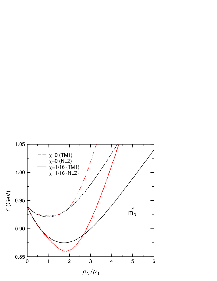
Figure 2: Comparison of energies per particle calculated within the TM1 and NLZ models for $\chi=0$ and $1/16$.

Figures 1, 2 show the energies per particle of $\overline{N}N$ matter calculated within the TM1 and NLZ models. The coupling constants of $\overline{N}$ interactions are fixed by the G–parity transformation (see Eq. (19)). Different curves corresponds to different values of antinucleon concentration $\chi$. Dashed lines in Fig. 1 represent the results for the case $\chi=1/16$ . It is seen that nucleonic matter becomes more bound after inserting a certain fraction of antibaryons. The maximal binding takes place at $\chi=1$ i.e. for the ”baryon–free” matter with net baryon density equal to zero. As one can see from Eqs. (33), (36), the repulsive vector contribution to the energy density vanishes in this case ($\omega_{0}=0$), therefore, the behavior of $\epsilon(\rho_{N})$ is determined only by the counterbalance of scalar attraction and effects of Fermi motion. It is interesting to note that such baryon–free $\overline{N}N$ matter is fully symmetric with respect to interchanging nucleons and antinucleons. Thus, there is absolutely no reason that the $N$ and $\overline{N}$ coupling constants would violate the G–parity symmetry.

To illustrate the model dependence of the results, in Fig. 2 we compare predictions of the TM1 and NLZ models for $\chi=0$  and $\chi=1/16$. One can see that the NLZ parametrization predicts larger binding of the $\overline{N}N$ matter at densities $\rho_{N}\sim 2\rho_{0}$ . The calculated parameters of bound states for $\chi=0$  (pure nucleonic matter), 1/16 and 1 are presented in Table 2.

Table 2: Characteristics of bound states of pure nucleonic matter ($\chi=0$) as well as the $\overline{N}N$ matter predicted by the TM1 and NLZ models.

Model	TM1			NLZ
$\chi$	0	$1/16$	1	0	$1/16$	1
$\rho_{N}/\rho_{0}$	0.99	1.75	4.99	1.01	1.84	4.04
$\epsilon$ (MeV)	922	875	449	923	860	412
$m_{N}^{*}$ (MeV)	593	393	90	544	224	42

By using Eq. (40) and the values of minimal energies per particle given in this table (for $\chi=1/16$), one can estimate the binding energy of a bound $\overline{p}\,+^{16}{\rm O}$  system. This leads to the result

$$BE\hskip 1.0pt(^{16}_{\hskip 3.0pt\overline{p}}{\rm O})=\left\{\begin{array}[]{ll}1070\,{\rm MeV{}}&(\mbox{\rm TM1})\,,\\ 1330\,{\rm MeV{}}&({\rm NLZ})\,.\end{array}\right.$$ (41)

On the other hand, applying the formalism of Sect. II to a finite system ¹⁶$\scriptstyle\overline{p}$ O Bue02 gives for its binding energy 1159  MeV (TM1) and 828 MeV (NLZ2). Comparison of these results shows influence of the finite size (surface), rearrangement (polarization) and Coulomb effects which are not taken into account in the infinite matter calculations.

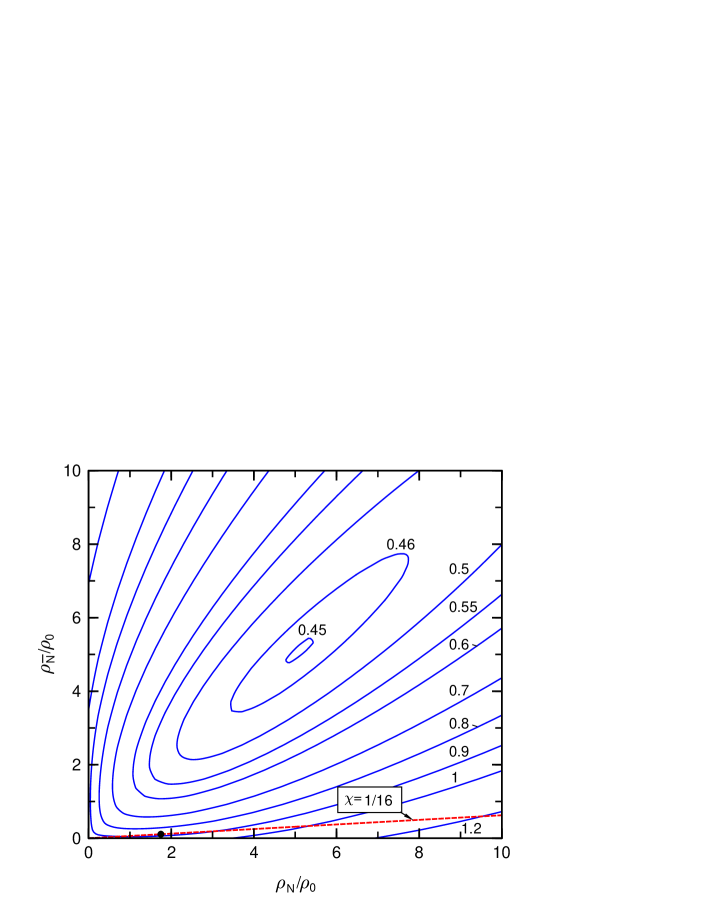
Figure 3: Contours of energy per particle (shown in GeV near the corresponding curves) on the $\rho_{N}-\rho_{\overline{N}}$  plane, calculated within the TM1 model. The dashed line corresponds to states with $\chi=1/16$ . Solid point shows position of minimal $\epsilon$ on this line.

More detailed results for the $\overline{N}N$ matter are represented in Fig. 3 in the form of contour plots of $\epsilon\hskip 1.0pt(\rho_{N},\rho_{\overline{N}})$ on the plane $\rho_{N}-\rho_{\overline{N}}$  calculated within the TM1 model. The states with fixed $\chi$ lie on straight lines going from the origin of the plane. The maximal binding, about 490 MeV per particle, is predicted for symmetric systems with $\rho_{\overline{N}}=\rho_{N}\simeq 5\hskip 1.0pt\rho_{0}$ . Most likely, the hadronic language is not valid at such high densities and the quark–antiquark degrees of freedom are more appropriate in this case.

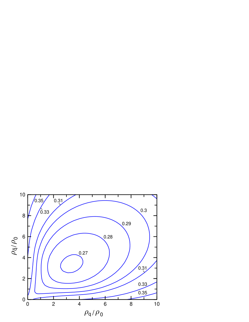
Figure 4: Contours of energy per particle, $\epsilon=E/(N_{q}+N_{\bar{q}})$ , (shown in GeV near the corresponding curves) of cold quark–antiquark matter calculated within the SU(2) NJL model Mis99 . The horizontal (vertical) axis corresponds to the total density of $u+d$ quarks (antiquarks) in units of $\rho_{0}=0.15$ fm^-3 .

Strong binding effects can also be expected in a deconfined $q\overline{q}$ matter. In Refs. Mis99 ; Mis00 we have performed calculations for such matter within the generalized Nambu–Jona-Lasinio (NJL) model. As an example, Fig. 4 shows energy per particle, $\epsilon=E/(N_{q}+N_{\bar{q}})$, for nonstrange isospin–symmetric $q\bar{q}$ matter at zero temperature. Here $N_{q}\,(N_{\bar{q}})$ denotes the total number of $u,d$ quarks (antiquarks). The figure displays contour plots of $\epsilon\hskip 1.0pt(\rho_{q},\rho_{\bar{q}})$ predicted by the SU(2) NJL model (for details, see Ref. Mis99 ). The binding in this case is generated by an attractive interaction in the scalar–pseudoscalar channel. Again, one can see that the strongest binding is predicted for the baryon–symmetric case $\rho_{q}=\rho_{\bar{q}}$ . The maximum binding energy per $q\bar{q}$ pair is

$$BE\simeq(m_{q}^{\rm vac}-270\,{\rm MeV})\times 2\simeq 60\,{\rm MeV}\,,$$ (42)

where $m_{q}^{\rm vac}\simeq 300$ MeV is the constituent mass of light quarks in the vacuum. Approximately three times larger binding energies have been found in Ref. Mis00 for cold quark–antiquark matter with admixture of strange $s,\bar{s}$ quarks. On the basis of this finding, in Refs. Mis99 ; Mis00 we have predicted possible existence of new metastable systems, mesoballs, consisting of many quarks and antiquarks in a common ”bag”. Such systems are characterized by a small (or zero) baryon number and their decay should occur mainly via emitting pions from the surface. It is interesting to note that multi–quark–antiquark clusters were also predicted Buc79 on the basis of the MIT bag model. It is instructive to compare the value (42) with the binding energy of baryon–symmetric $\overline{N}N$ matter calculated within the RMF model. Using Table 2 for the case $\chi=1$ , we get the binding energy per quark–antiquark pair, $2\hskip 1.0pt(m_{N}-\epsilon)/3\simeq 326\,(350)$  MeV, within the TM1 (NLZ) model. Therefore, the hadronic approach may overestimate real binding energies of cold and dense baryon–free matter by a factor $\sim 5$ .

Figure 5: Energy per particle of the $\overline{N}N$ matter versus the nucleon density at fixed $\chi=1/16$ . Different curves correspond to the TM1 calculation at different values of the parameter $\xi$ characterizing deviation of the $\overline{N}$ coupling constants from the G–parity motivated values.

As noted above, the G–parity symmetry may be violated in a dense baryon–rich matter. As a consequence, the G–parity motivated choice of antibaryon coupling constants, Eq. (19), may overestimate binding energies of the $\overline{B}N$ matter. To elaborate on this issue, we have performed an analogous calculation, but with reduced couplings $g_{\sigma\overline{B}}\,,~{}g_{\omega\overline{B}}$  as defined in Eq. (20). The results of calculations within the TM1 model for different values of $\xi$ are presented in Fig. 5. It shows the energy per particle of $\overline{N}N$ matter with $\chi=1/16$. The lower curve corresponds to the case of the exact G–parity symmetry. One can see that a reduction of $\xi$ results in a smaller binding and compression of the $\overline{N}N$ matter. However, the admixture of antinucleons becomes relatively unimportant only at very small antinucleon couplings, corresponding to $\xi\hskip 1.0pt<0.25$ . It is shown below that the same conclusion follows from more refined calculations for the finite ¹⁶$\scriptstyle\overline{p}$ O system.

Table 3: The parameters of the TM1 and NLZ models in the hyperonic sector. The remaining parameters are given in Table 1.

	$m_{\overline{\Lambda}}\,({\rm MeV})$	$m_{\sigma^{*}}\,({\rm MeV})$	$m_{\phi}\,({\rm MeV})$	$g_{\sigma\overline{\Lambda}}$	$g_{\omega\overline{\Lambda}}$	$g_{\rho\hskip 1.0pt\overline{\Lambda}}$	$g_{\sigma^{*}\overline{\Lambda}}$	$g_{\phi\overline{\Lambda}}$
NLZ	1116	975	1020	6.23	$-8.61$	0	6.77	6.09
TM1	1116	975	1020	6.21	$-8.41$	0	6.67	5.95

We end this section by considering cold nucleonic matter with admixture of antihyperons $\overline{Y}=\overline{\Lambda},\,\overline{\Sigma}\ldots$ As proposed in Ref. Sch96 , the observed data on $\Lambda\Lambda$ interaction can be reproduced within the RMF model by including additional scalar ($\sigma_{*}$) and vector ($\phi$) meson fields coupled only to hyperons. By the same reason, to take into account the interaction between antihyperons in the $\overline{Y}N$ matter, we generalize the Lagrangian (4) by introducing the additional terms 

$$\delta{\cal{L}}_{YY}= \frac{1}{2}\left(\partial^{\mu}\sigma_{*}\partial_{\mu}\sigma_{*}-m_{\sigma}^{2}\sigma_{*}^{2}\right)-\frac{1}{4}\phi^{\mu\nu}\phi_{\mu\nu}+\frac{1}{2}m^{2}_{\phi}\phi^{\mu}\phi_{\mu}+$$ (43)

$$+\overline{\psi}_{\overline{Y}}\left(g_{\sigma_{*}\overline{Y}}\hskip 1.0pt\sigma_{*}-g_{\phi{\overline{Y}}}\hskip 1.0pt\phi^{\mu}\gamma_{\mu}\right)\psi_{\overline{Y}}\,.$$

In our calculations of the $\overline{\Lambda}N$ matter and bound $\overline{\Lambda}$–nuclear systems we use the values of parameters suggested in Ref. Sch96 . The $\overline{\Lambda}$–meson couplings were obtained from the $\Lambda$–meson coupling constants by using the G–parity transformation.

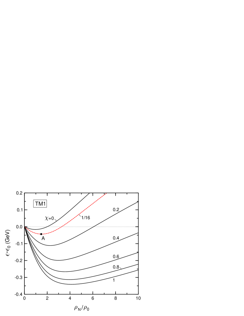
Figure 6: Energy per particle of $\overline{\Lambda}N$ matter versus the nucleon density calculated within the TM1 model. Different curves correspond to different values of the $\overline{\Lambda}$ concentration $\chi=\rho_{\overline{\Lambda}}/\rho_{N}$ . The curves are shifted along the vertical axis by a $\chi$–dependent value $\epsilon_{0}=\lim\limits_{\rho_{N}\to 0}\epsilon$ . Point A marks the position of energy minimum for $\chi=1/16$ .

Table 4: Characteristics of bound states of pure nucleonic matter ($\chi=0$) as well as the $\overline{\Lambda}N$–matter predicted by the TM1 models.

$\chi$	0	$1/16$	1/4	1
$\rho_{N}/\rho_{0}$	0.99	1.47	2.49	4.08
$\epsilon_{0}-\epsilon$ (MeV)	16	44	135	252
$m_{N}^{*}$ (MeV)	593	456	257	44
$m_{\overline{\Lambda}}^{*}$ (MeV)	905	812	662	420

It is easy to see that the hyperon-hyperon interactions lead to the following effects. First, the gap equation for the antihyperon effective mass is modified (as compared to Eq. (29)) due to the additional $\sigma_{*}$ field:

$$m_{\overline{Y}}^{*}=m_{\Lambda}-g_{\sigma\overline{Y}}\sigma-g_{\sigma_{*}\overline{Y}}\sigma_{*}\,.$$ (44)

Second, the energy density of the $\overline{Y}N$ matter contains now the additional contribution of $\sigma_{*}$  and $\phi$  mesons,

$$\delta e_{YY}=\frac{1}{2}\left(m_{\sigma_{*}}^{2}\sigma_{*}^{2}+m_{\phi}^{2}\phi_{0}^{2}\right)\,.$$ (45)

Figure 6 shows the energy per particle of the $\overline{\Lambda}N$ matter, calculated within the TM1 model, generalized in accordance with Eqs. (44)–(45), with parameters listed in Tables 1, 3. To compare results for different $\chi$ , the energy per particle is shifted by a corresponding vacuum value $\epsilon_{0}$ defined in Eq. (39). The calculated parameters of bound states are given in Table 4. Comparison with results obtained earlier for the $\overline{N}N$ matter shows that binding energies and equilibrium densities are noticeably smaller in the $\overline{\Lambda}N$ case. For example, the binding energy predicted for the ¹⁶$\scriptstyle\overline{\Lambda}$ O  ”nucleus” equals approximately $44\times 17\simeq 748$  MeV which is about 30% smaller than for ¹⁶$\scriptstyle\overline{p}$ O bound state. This difference is explained by a smaller scalar coupling of $\overline{\Lambda}$ particles as compared to antinucleons ($g_{\sigma\overline{\Lambda}}/g_{\sigma\overline{N}}\simeq 2/3$) .

IV Finite antibaryon–nuclear systems

IV.1 Light nuclear systems with antiprotons

The nucleus ¹⁶O is the lightest nuclear system for which the RMF approach is considered to be reliable. This nucleus is included into the fit of the effective forces NL3 and NLZ2. Therefore, we choose this nucleus as a basic system to study the antibaryon–nuclear bound states. First, let us consider an antiproton bound in a ¹⁶O nucleus. For clarity we use the notation ¹⁶$\scriptstyle\overline{p}$ O for such a combined system. A priori it is unclear which quantum numbers has the lowest bound state. We first assume that this is the $\frac{1}{2}^{+}$ state and later on we shall check this assumption. Results of our self-consistent calculations for both ¹⁶O and ¹⁶$\scriptstyle\overline{p}$ O are presented in Fig. 7.

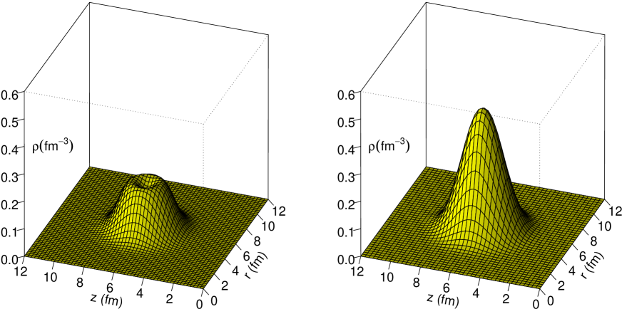
Figure 7: 3D plots of nucleon density in the ¹⁶O nucleus (left) and in the bound $\overline{p}\hskip 1.0pt\hskip 1.0pt+^{16}$O system (right) calculated within the NL3 model.

It shows 3D plots of the nucleon densities for the G–parity motivated antiproton couplings ($\xi$=1). One can see that inserting an antiproton into the nucleus gives rise to a dramatic rearrangement of nuclear structure. This effect has a simple origin. As explained above, the antiproton contributes with the same sign as nucleons to the scalar density (see Eq. (21)), but with the negative sign to the vector density. This leads to an overall increase of attraction and decrease of repulsion for surrounding nucleons. To maximize attraction, protons and neutrons move to the center of the nucleus, where the antiproton has its largest occupation probability. This leads to a strong compression of the nucleus.

Figure 8: The left panel represents the sum of proton and neutron densities as function of nuclear radius for ¹⁶O without (top) and with an antiproton. The left and right parts of the upper middle panel show separately the proton and neutron densities, the lower part of this panel displays the antiproton density (with minus sign). The right panel shows the scalar (negative) and vector (positive) parts of the nucleon potential. Small contributions shown in the lower row correspond to the isovector ($\rho$–meson) part.

Figure 8 shows the densities and potentials for ¹⁶O with and without the antiproton. For normal ¹⁶O all RMF parametrizations considered produce very similar results. The presence of the antiproton changes drastically the structure of the nucleus. Depending on the parametrization, the sum of proton and neutron densities reaches a maximum value of $(2-4)\,\rho_{0}$ , where $\rho_{0}\simeq 0.15$ fm^-3 is the normal nuclear density. The largest compression is predicted by the TM1 model. This follows from the fact that this parametrization gives the softest equation of state as compared to other forces considered here. According to our calculations, the difference between proton and neutron densities is quite large, which leads to an increase in symmetry energy. The reason is that protons, though they feel additional Coulomb attraction to the antiproton, repel each other. As a consequence, neutrons are concentrated closer to the center than protons and the symmetry energy increases.

Figure 9: Left panels: radial profiles of the vector ($\rho_{j}$) and scalar ($\rho_{Sj}$) densities of antiproton ($j=\overline{p}$) and nucleons ($j=N$) in the ground state of ${}^{16}_{\hskip 3.0pt\overline{p}}$O as predicted by the NLZ2 and NL3 calculations. Right panels show the corresponding profiles of the effective nucleon mass.

Figure 9 shows radial profiles of scalar and vector densities of nucleons and the antiproton in ¹⁶$\scriptstyle\overline{p}$ O . As compared to the normal ¹⁶O nucleus, absolute values of vector and scalar densities increase in the central region of the nucleus. This leads to a strong drop of the effective nucleon mass near the nuclear center , which in turn suppresses the local annihilation rate of the antiproton (see Sect. V).

Figure 10: Proton (left), neutron (middle) and antiproton (right) energy levels for the nucleus ¹⁶O with one antiproton and without it (rightmost columns in the left and middle panels).

Since nucleons feel a deeper potential due to the presence of the antiproton, their binding energy increases too. This can be seen in Fig. 10. The nucleon binding is largest within the NL3 parametrization. In the TM1 case, the $s1/2^{+}$ state is also deep, but higher levels are less bound as compared to the NL3 and NLZ2 calculations. This is a consequence of the smaller spatial extension of the potential in this case. The highest $s1/2^{-}$ level in the TM1 calculation (see Fig. 10) is even less bound than for the system without an antiproton.

For the antiproton levels, the TM1 parametrization predicts the deepest bound state with binding energy of about $1130$ MeV. The NL3 calculation gives nearly the same binding, while in the NLZ2 case, antiproton levels are more shallow and have smaller spacing. It should be noted that the antiprotons are more strongly bound than was obtained in Ref. Mao99 . This follows from the fact that here we consider both nucleons and the antinucleon self–consistently allowing the target nucleus to change its shape and structure due to the presence of the antiproton. The total binding energy of the ¹⁶$\scriptstyle\overline{p}$ O  system is predicted to be 828 MeV for NLZ2, 1051 MeV for NL3, and 1159 MeV for TM1. For comparison, the binding energy of the normal ¹⁶O nucleus is 127.8, 128.7 and 130.3 MeV in NLZ2, NL3, and TM1, respectively.

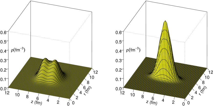
Figure 11: 3D plots of nucleon densities for the nucleus ⁸Be without (left) and with (right) antiproton calculated within the NL3 model.

As a second example, we investigate the effect of a single antiproton inserted into the ⁸Be nucleus. In this case only the NL3 parametrization was used (the effect is similar for all three RMF models). The normal ⁸Be nucleus is not spherical, exhibiting a clearly visible $\alpha-\alpha$ structure with the deformation $\beta_{2}\simeq 1.20$ in the ground state. As one can see from Fig. 11, inserting an antiproton gives rise to the compression and change of nuclear shape, which results in a much less elongated nucleus with $\beta_{2}\simeq 0.23$. Its maximum density increases by a factor of three from $1.3\hskip 1.0pt\rho_{0}$ to $4.1\hskip 1.0pt\rho_{0}$ . The cluster structure of the ground state completely vanishes. A similar effect has been predicted in Ref. Aka02 for the $K^{-}$ bound state in the ⁸Be nucleus. In our case the binding energy increases from $52.9$ MeV (the experimental value is $56.5$ MeV) to about $700$ MeV.

Figure 12: The profiles of net baryon density, $\rho_{N}-\rho_{\overline{p}}$ , in the $\overline{p}\,+^{4}$He (left) and $\overline{p}\,+^{16}$O (right) systems, calculated within the NLZ2 model.

Figure 12 represents profiles of the net baryon density i.e. the sum of the proton and neutron densities minus the antiproton density. For both considered systems, there is a dip in the center surrounded by the region with baryon density increased as compared to normal nuclei.

Table 5: Total binding energies of $\overline{p}+^{16}$O system with antiproton occupying different states.

$J_{z}^{\pi}$	$1/2^{+}$	$3/2^{-}$	$1/2^{-}$	$1/2^{-}$
NL3	-1051	-1008	-920	-780
NLZ2	-828	-938	-804	-876

Now we address the question of wether the antiproton $1/2^{+}$ state is energetically the most favorable configuration of the ¹⁶$\scriptstyle\overline{p}$ O  system or not. To answer this questions, we put the antiproton into various states and calculate the total binding energy. The results are shown in Table 5. In the case of NL3, the lowest $1/2^{+}$ state indeed corresponds to the configuration with lowest energy. However, within the NLZ2 calculation a state with the antiproton in the $3/2^{-}$ state corresponds to the ground state of the system.

Figure 13: 3D plot of nucleon density in the in the bound $\overline{\Lambda}\,+^{16}$O system calculated with the NLZ model.

The $3/2^{-}$ state has a different spatial distribution and thus, leads to a different shape of the potential felt by nucleons. So, even though the antiproton in the $3/2^{-}$ state is less bound than in the $1/2^{+}$ state, nucleons become more bound in this case and the binding energy of the whole system increases.

IV.2 Light systems with antilambdas

Figure 14: Radial profiles of the net baryon density, $\rho_{N}-\rho_{\overline{\Lambda}}$ , in the $\overline{\Lambda}\,+^{4}$He (left) and $\overline{\Lambda}\,+^{16}$O (right) systems calculated with the NLZ model.

Bound states of nuclei with antihyperons are especially interesting because we expect longer life times in this case (see Sect. V). We performed calculations of the ⁴$\scriptstyle\overline{\Lambda}$ He and ¹⁶$\scriptstyle\overline{\Lambda}$ O  systems within the NLZ model. The assumed $\overline{\Lambda}$ couplings with the meson fields are given in Table 3.

Figure 13 shows the 3D plot of the sum of proton and neutron densities in the ¹⁶$\scriptstyle\overline{\Lambda}$ O  nucleus. Comparison with the results for the ¹⁶$\scriptstyle\overline{p}$ O  systems (see Fig. 7) shows noticeably lower nucleon densities in this case. However, we still predict significant compression of nuclei containing antihyperons. Figure 14 gives profiles of the net baryon density in the ⁴$\scriptstyle\overline{\Lambda}$ He and ¹⁶$\scriptstyle\overline{\Lambda}$ O  nuclei. It is interesting that the central density dip is even more pronounced here as compared to nuclei with antiprotons (see Fig. 12). This effect can be explained by a stronger localization of the antilambda due to its larger effective mass.

Figure 15: The profiles of densities and mean–field potentials in the bound $\overline{p}\hskip 1.0pt+^{16}$O system calculated with reduced antiproton coupling constants. The upper (lower) panel corresponds to the NL3 (NLZ2) model. Different curves correspond to different values of the parameter $\xi$  defined in Eq. (20). Shown are the nucleon densities (left), antiproton densities (middle) and scalar and vector potentials for nucleons (right). Note, that at $\xi<1$ the antiproton potentials are smaller due to reduced $\overline{p}$ couplings.

IV.3 Calculations with reduced antibaryon couplings

As was pointed out earlier, the G–parity transformation may not work on the mean–field level. Therefore, we have performed calculations of bound $\overline{p}+A$ systems with reduced antiproton couplings to mean meson fields. Figure 15 shows the results for the ¹⁶$\scriptstyle\overline{p}$ O  nucleus obtained for several values of the parameter $\xi$ introduced in Eq. (20).

Figure 16: Binding energy of ${}^{16}_{\hskip 3.0pt\overline{p}}$O calculated in the TM1 and NLZ models as a function of the parameter $\xi$ .

One can see that at $\xi\gtrsim 0.25$, the compressed shape of the nucleus is not very much affected. The largest compression, of course, occurs for $\xi=1$, i.e. in the case of the exact G–parity. At $\xi$ smaller than $0.05$ (NL3) or $0.01$ (NLZ2), the nucleon density profiles practically coincide with the density distribution of the normal ¹⁶O nucleus. On the other hand, the antiproton density profile becomes rather flat in this case. Somewhere in between, there exists a critical $\xi$ value separating these two regimes. Detailed calculations with different $\xi$ show that there is no smooth transition but rather an abrupt jump. This is an indication that, to a large extent, the shell effects control the structure of these systems.

Figure 17: Same as in Fig. 15 but for ⁴He with an antiproton.

The results of these calculations show that the conclusions made in Ref. Bue02 and in the present work do not strongly depend on the actual values of $g_{\sigma\overline{N}}$ and $g_{\omega\overline{N}}$. As a consistency check, we verified that at $\xi\to 0$ the binding energy of ¹⁶$\scriptstyle\overline{p}$ O  goes to the value of normal ¹⁶O . This is demonstrated in Fig. 16 where one can see strong increase of the binding energy for $\xi\gtrsim 0.1$ .

Similar results take place for the $\overline{p}\hskip 1.0pt+^{4}$He system. They are presented in Fig. 17. Of course, this is system is rather small and the mean-field approximation may be not accurate in this case. Nevertheless, we expect to get a qualitative picture even for such a light system. At $\xi=1$ the nucleon density in the ⁴$\scriptstyle\overline{p}$ He nucleus reaches a maximum value of about $6\hskip 1.0pt\rho_{0}$ which is noticeably larger than in ¹⁶$\scriptstyle\overline{p}$ O . As in the case of ¹⁶$\scriptstyle\overline{p}$ O , depending on the $\xi$ value, there are two different configurations of the bound system, namely a highly compressed one and the other resembling normal helium plus a quasi free antiproton. For both RMF models, the reduction of antiproton coupling constants up to $\xi\simeq 0.25$ does not produce a strong effect in the density distribution.

IV.4 Rearrangement of nuclear structure and Dirac sea

Figure 18: Proton and antiproton potentials as well as corresponding single–particle levels for the systems ⁴He, $\overline{p}\,+^{4}$He (left side) and ¹⁶O, $\overline{p}\,+^{16}$O (right side) calculated within the NLZ2 model. The full and open dots in the Dirac sea show the most bound occupied and vacant states, respectively.

The presence of an antiproton within a light nucleus leads to a drastic rearrangement of its structure and to the polarization of the Dirac sea. We illustrate this effect in Fig. 18, where the effective potentials and single–particle levels are shown for helium and oxygen, in each case with and without an antiproton. A hole at the deepest bound level in the lower well corresponds to a positive energy antiproton. After inserting an antiproton the nuclear structure is strongly rearranged. Both the nucleonic as well as the antiparticle states become deeper which gives rise to increase of the binding energy by several hundred MeV. The lower well in the case of the $\overline{p}\,+^{4}$He system is very narrow and its bottom overlaps with the positive energy well. The uncertainty relation prevents, however, the strongest bound antiparticle and particle states to be very close in energy. The lower well in the case of oxygen also becomes narrower as compared with normal ¹⁶O nucleus.

The rearrangement of the Dirac sea due to the presence of an antiproton leads to increasing number of negative energy states. The spin–orbit potential for antiparticles is very small, because, in contrast to nucleons, scalar and vector potentials for antiprotons nearly cancel each other . Still, there are gaps between the antiparticle levels of the order of a hundred MeV (see Fig. 10). This is a consequence of a smaller width of the lower well as compared to the negative energy well in the normal nucleus.

IV.5 Heavy nuclei containing antibaryons

In this section we investigate the effect of antiprotons and antilambdas inserted into heavy nuclei. Because of larger radii of these objects ($R\gtrsim 7$ fm), one may expect appearance of a local compression zone in the central region instead of a more homogeneously compression in lighter systems. This is exactly what follows from our calculation. Figure 19 shows the sum of proton and neutron densities, for the case of doubly–magic lead nucleus with one deeply–bound antiproton. Due to the presence of an antiproton, a small core of highly compressed nuclear matter appears at in the center of the ²⁰⁸$\scriptstyle\overline{p}$ Pb  nucleus. In addition, the lead nucleus becomes deformed and acquires a prolate shape. As shown in Fig. 20 a similar structural change occurs when implementing the $\overline{\Lambda}$ particle into the ²⁰⁸Pb target.

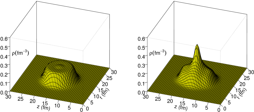
Figure 19: 3D plots of nucleon density in the ²⁰⁸Pb nucleus (left) and in the bound $\overline{p}\,+^{208}$Pb  system calculated within the NL3 model.

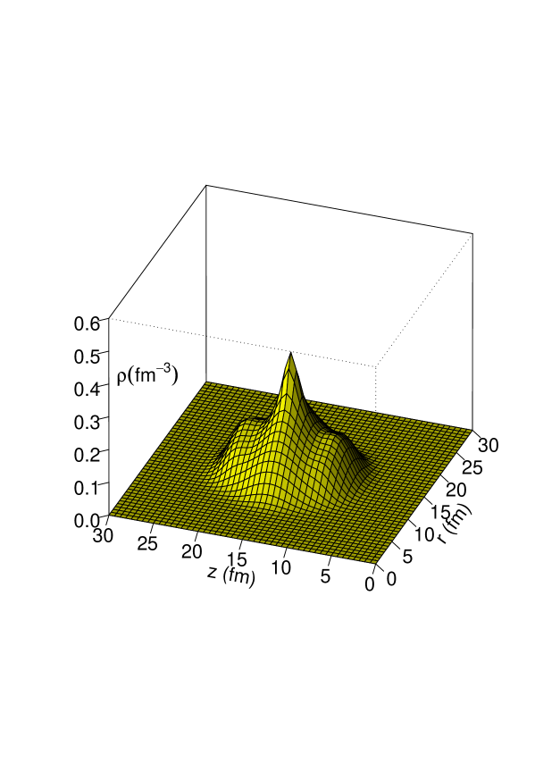
Figure 20: 3D plots of nucleon density in the bound $\overline{\Lambda}\,+^{208}$Pb system calculated within the NLZ model.

Figure 21 shows single–particle spectra of protons, neutrons and antiprotons in the normal lead as well as in the bound ²⁰⁸$\scriptstyle\overline{p}$ Pb  and ²⁰⁸$\scriptstyle\overline{\Lambda}$ Pb nuclei. One can see that implementing antiparticles results in a strong change of shell structure. Due to the axial deformation, the system looses its degeneracy and the shell structure becomes partly washed out. Only the $1/2+$ and $3/2-$ levels exhibit large binding. The deepest antibaryon states have binding energies of more than 900 (600) MeV in the case of the ²⁰⁸$\scriptstyle\overline{p}$ Pb (²⁰⁸$\scriptstyle\overline{\Lambda}$ Pb) system. On the other hand, some of the single–particle states become even less bound in the lead nucleus with antibaryons.

These results can be qualitatively understood from the fact that the nucleon potential in the center of the bound system is very deep but narrow. Two effects prevent deeper binding of single–particle levels. First, a narrow potential gives rise to large uncertainties in particle momenta. This in turn increases the kinetic energies of particles and therefore, reduces their binding. Second, the single–particle states with larger angular momenta are mainly localized at larger radii and thus do not have much overlap with the deep central region of the potential.

Figure 21: Single–particle proton (left), neutron (middle) and antiproton spectra for the systems ²⁰⁸Pb, $\overline{p}\,+^{208}$Pb (NL3 forces) and $\overline{\Lambda}\,+^{208}$Pb (NLZ2 set).

The total binding energy of the ²⁰⁸$\scriptstyle\overline{p}$ Pb  nucleus predicted by the NL3 calculation equals 2412 MeV or 11.5 MeV per particle. This is significantly smaller than 61.8 MeV per particle in the ¹⁶$\scriptstyle\overline{p}$ O  system. Furthermore, the total energy gain in the binding energy after inserting an antibaryon into the ²⁰⁸Pb nucleus (780 MeV) is smaller than in the ¹⁶O case (920 MeV).

Figure 22: The profiles of nucleon density in the ${}^{208}_{\hskip 6.0pt\overline{p}}$ Pb system at different values of the paramater $\xi$ . The left and right panels correspond, respectively, to the equatorial and coaxial planes.

Figure 22 shows the nucleon density profiles in the ²⁰⁸$\scriptstyle\overline{p}$ Pb  system calculated with $\xi=1,0.5$ and 0 (the normal Pb nucleus). Because of the axial deformation we show separately the profiles for radial (equatorial) and coaxial planes. This figure demonstrates a very interesting behavior. Contrary to a naive expectation, reducing $\xi$ from 1 to 0.5 leads to increasing density of the central core . We believe that this can be explained by the competition of two opposite trends taking place at decreasing $\xi$ . The first one is the reduction of the binding potential while the second one is the increase of the antiproton effective mass. The second effect leads to a stronger localization of the antiproton wave function near the minimum of the effective potential. As a consequence, the potential acting on surrounding nucleons increases in the central regions.

IV.6 Systems containing several antibaryons

It is amazing to consider nuclear systems with more than one trapped antibaryon. For instance let us consider doubly–magic oxygen containing different numbers of antiprotons, namely $N_{\overline{p}}=2,4,6,8$  and 10.

Figure 23: Net baryon density, $\rho_{N}-\rho_{\overline{p}}$, for the ¹⁶O nucleus with 2, 4, 6, 8 and 10 antiprotons, calculated within the NL3 model.

The corresponding baryon densities are shown in Fig. 23. The total binding energies for the systems containing 2, 4, 6, 8 and 10 antiprotons are 1541, 2792, 3847, 5006, and 6300 MeV, respectively. As we can expect, with increasing number of antiprotons, the region of reduced net baryon density becomes broader. In the case $N_{\overline{p}}=10$ one can see a qualitative change of nuclear structure, with appearance of a baryon density peak in the center region and a zone of reduced density at the nuclear periphery.

Figure 24: The system $\alpha-\overline{\alpha}$ calculated within the NLZ2 (solid line) and NL3 (dotted line) models. Shown are baryon and antibaryon densities (left) as well as the scalar potential and energies of the lowest single–particle states (right). The dashed line shows the nucleon density of the normal $\alpha$ particle calculated within the NLZ2 model.

One can also think of most extreme case of finite systems with equal numbers of baryons and antibaryons, i.e. about systems with total baryon number $B=0$ . These systems can be called self–conjugate nuclei, since their charge conjugation leads to the same object. Let us first consider the bound $\alpha-\overline{\alpha}$ system. As seen in Fig. 24, the (anti)particle densities in this system reach about $10\hskip 1.0pt\rho_{0}$ . Of course, one should expect a breakdown of the RMF model with nucleonic degrees of freedom at such high densities. Most probably the (anti)baryons will dissolve into a deconfined state of cold and dense $q\overline{q}$ matter (see Sect. III).

Figure 25: The system ¹⁶O–${}^{16}\overline{{\rm O}}$ calculated within the NL3 model. The dotted lines show the baryon and antibaryon densities (left) as well as the scalar potential and the lowest single–particle states (right). The dashed line represents the nucleon density of the normal ¹⁶O nucleus.

Due to the full symmetry between baryons and antibaryons (or quark and antiquarks) such systems have both vanishing baryon and electric charges. Accordingly, the vector fields, namely the $\omega$ meson and Coulomb fields, vanish too. Only the scalar density and with it the scalar potential are nonzero in a symmetrical system. Since nucleons and antinucleons have the same scalar potential, they can occupy the same single–particle states. In this case the spatial parts of the wave functions of protons, neutrons, antiprotons and antineutrons are identical. Hence, the spatial overlap between particles and antiparticles is maximal. On the other hand, due to the very high density of baryons and antibaryons, the effective masses are very small in the core region. The calculated binding energy of the $\alpha-\overline{\alpha}$ system is very large, it is 2649 MeV for NL3 and 2235 MeV for NLZ2. This is about 100 times the value for a single $\alpha$ particle and 40 times the binding energy of normal ⁸Be nucleus.

As a second example we consider the ¹⁶O–${}^{16}\overline{{\rm O}}$ system. The calculated profiles of (anti)nucleon density and scalar potential are shown in Fig. 25 . In this case we predict formation of a highly compressed system with maximal nucleon and antinucleon densities of about $5\rho_{0}$ . One can see in Figs. 24–25 that radial profiles of the scalar potential in symmetric $A+\overline{A}$  systems are noticeably broader as compared to the (anti)nucleon density distributions. Such a behavior follows from the finite range of $\sigma$ meson field (see Eq. (11)).

V Annihilation of deeply bound antibaryons

V.1 $\overline{N}N$ annihilation in vacuum

At low energies the total cross section of $\overline{p}p$ annihilation in vacuum can be well approximated as Dov92

$$\sigma^{\rm\hskip 1.0ptann}_{\overline{p}p}=C+\frac{D}{~{}v_{\rm rel}}\,,$$ (46)

where $v_{\rm rel}$ is the relative velocity of $\overline{p}$  with respect to the proton, $C=38$ mb, $D=35\,{\rm mb}\cdot{\rm c}$ . In the following we neglect the isotopic and Coulomb effects assuming that $\overline{p}p$ and $\overline{p}n$ annihilation cross sections are approximately equal. Using this approximation we discuss below the isotopically averaged $\overline{N}N$ interactions.

When the $\overline{N}N$ c.m. energy $\sqrt{s}$ is close to the vacuum threshold value, i.e. at $\sqrt{s}\to 2m_{N}\simeq 1.88$ GeV, the relative velocity becomes small and the $\overline{N}N$ annihilation cross section is approximately proportional to $1/v_{\rm rel}$ . This limiting case of annihilation ”at rest” ($v_{\rm rel}\to 0$) has been extensively studied in Refs. Bac83 ; Sed88 ; Obe97 ; Cry94 ; Cry96 ; Ams98 ; Cry03 . Experimental data on many exclusive annihilation channels $\overline{p}p\to c\to n_{\pi}\pi$ are also available. Here intermediate states $c$ include direct pions as well as heavy mesons $\eta\hskip 1.0pt(547),\rho\hskip 1.0pt(770),\omega\hskip 1.0pt(782)\ldots$

Table 6: Exclusive channels of $\overline{p}p$ annihilation at rest in vacuum

$n_{\pi}$	$c$	$\sqrt{s}_{\rm thr}({\rm GeV})$	$B_{c}(\%)$	Refs.
2	$2\pi^{0}$	0.27	0.07	Cry03
	$\pi^{+}\pi^{-}$	0.28	0.31	Ams98
3	$(3\pi^{0})_{\rm\hskip 1.0ptdir}$	0.41	0.7	Cry03
	$(\pi^{+}\pi^{-}\pi^{0})_{\rm\hskip 1.0ptdir}$	0.42	1.8	Ams98
	$\pi^{0}\rho^{0}$	0.91	1.7	Ams98
	$\pi^{\pm}\rho^{\mp}$	0.91	3.4	Ams98
4	$(4\pi^{0})_{\rm\hskip 1.0ptdir}$	0.54	0.5	Cry03
	$(\pi^{+}\pi^{-}\hskip 1.0pt2\pi^{0})_{\rm\hskip 1.0ptdir}$	0.55	7.8	Bac83 ; Sed88 ; Ams98
	$(2\pi^{+}2\pi^{-})_{\rm\hskip 1.0ptdir}$	0.56	4.2	Sed88 ; Obe97
	$\pi^{0}\omega$	0.92	0.6	Ams98
	$\pi^{+}\pi^{-}\rho^{0}$	1.05	3.6	Sed88
	$\rho^{+}\rho^{-}$	1.54	0.9	Sed88
5	$(5\pi^{0})_{\rm\hskip 1.0ptdir}$	0.68	0.5	Cry94 ; Cry96
	$(\pi^{+}\pi^{-}\hskip 1.0pt3\pi^{0})_{\rm\hskip 1.0ptdir}$	0.69	20.1	Bac83 ; Cry94 ; Cry03
	$(2\pi^{+}2\pi^{-}\pi^{0})_{\rm\hskip 1.0ptdir}$	0.70	10.4	Sed88 ; Cry94 ; Ams98
	$2\pi^{0}\eta$	0.82	0.7	Cry94
	$\pi^{+}\pi^{-}\eta$	0.83	1.3	Cry94
	$2\pi^{0}\omega$	1.05	2.6	Cry03
	$\pi^{+}\pi^{-}\omega$	1.06	6.6	Ams98
	$\rho^{0}\omega$	1.55	2.3	Ams98
6	$(\pi^{+}\pi^{-}4\pi^{0})_{\rm\hskip 1.0ptdir}$	0.82	1.9	Bac83 ; Sed88
	$(2\pi^{+}2\pi^{-}2\pi^{0})_{\rm\hskip 1.0ptdir}$	0.83	13.3	Bac83 ; Cry03
	$(3\pi^{+}3\pi^{-})_{\rm\hskip 1.0ptdir}$	0.84	2.0	Sed88
	$\omega\eta$	1.32	1.5	Cry03
	$2\omega$	1.54	3.0	Cry03
7	$(2\pi^{+}2\pi^{-}3\pi^{0})_{\rm\hskip 1.0ptdir}~{}~{}$	0.97	4.0	Bac83 ; Cry03
	$(3\pi^{+}3\pi^{-}\pi^{0})_{\rm\hskip 1.0ptdir}$	0.98	1.9	Sed88
	$\pi^{0}\omega\eta$	1.47	1.0	Cry03

Various channels of the $\overline{p}p$ annihilation at rest are listed in Table 6. They are sorted into groups with different final pion multiplicities $n_{\pi}$ . The most important exclusive channels $c$ are given in the second column. In the third column we give the corresponding threshold energies in the c.m. frame (i.e. the total mass of particles in the intermediate state). The fourth column shows the observed branching ratio of a given channel $c$:

$$B_{c}=\sigma_{\overline{p}p\to c}/\sigma^{\rm\hskip 1.0ptann}_{\overline{p}p}\,.$$ (47)

In the last column we give references to publications where experimental information on branching ratios has been found. The subscripts ”dir” in the second column mean that only nonresonant contributions are given in the corresponding line. For example, the branching ratio of the $(\pi^{+}\pi^{-}\pi^{0})_{\rm\hskip 1.0ptdir}$ channel has been calculated using the formula

$$B_{\overline{p}p\to(\pi^{+}\pi^{-}\pi^{0})_{\rm\hskip 1.0ptdir}}=B_{\hskip 1.0pt\overline{p}p\to\pi^{+}\pi^{-}\pi^{0}}-B_{\hskip 1.0pt\overline{p}p\to\pi^{0}\rho^{0}}-B_{\hskip 1.0pt\overline{p}p\to\pi^{\pm}\rho^{\mp}}\,,$$ (48)

where the first term in the r.h.s. is the total branching ratio of the reaction $\overline{p}p\to\pi^{+}\pi^{-}\pi^{0}$ and the two other terms give the contributions of the $\pi\rho$ intermediate states. Here we take into account that $\rho\to 2\pi$ is the dominant channel of the $\rho$ meson decay Pdg02 . The channels $c=3\pi^{0},\hskip 1.0pt4\pi^{0},\hskip 1.0pt\pi^{+}\pi^{-}4\pi^{0},\hskip 1.0pt3\pi^{+}3\pi^{-}$ and $3\pi^{+}3\pi^{-}\pi^{0}$ are classified as direct, because no resonance contributions have been found there. In Table 6 we include only main annihilation channels with $B_{c}>0.5\hskip 1.0pt\%$ (for $n_{\pi}>2$). We do not separate resonances in channels with total number of intermediate mesons exceeding three.

V.2 Kinetic approach to annihilation in medium

Let us first consider annihilation of slow antibaryons, $\overline{B}$ , in homogeneous nucleonic matter with a small admixture of antibaryons. Using again the mean–field approach we treat the $\overline{B}+N$ matter as a mixture of ideal Fermi gases of nucleons and antibaryons interacting with mean meson fields. Assuming that annihilation on multinucleon clusters is relatively small (see below), we consider here only the binary $\overline{B}N$ annihilation. Then the local rate of $\overline{B}$ annihilation per unit volume can be written as a sum over all $\overline{B}N$ annihilation channels with production of $n\geq 2$ mesons in the final state:

$$\frac{dN_{\rm ann}}{dtdV}=\sum_{n}\frac{dN_{\overline{B}N\to M_{1}\hskip 1.0pt\ldots\hskip 1.0ptM_{n}}}{dtdV}\,.$$ (49)

Here $M_{l}\hskip 1.0pt(l=1,\ldots,n)$ denote secondary mesons. In the following we disregard in–medium modifications of these mesons, assuming that their 4–momenta $k_{l}$ satisfy the mass–shell constraints, $k_{l}^{2}=m_{l}^{2}$ , with vacuum masses $m_{l}$ .

In the quasiclassical approximation one can describe the phase–space density of antibaryons ($i=\overline{B}$) and nucleons ($i=N$) by distribution functions $f_{i}(x,\bm{p})$ , where $x=(t,\bm{r})$ is the space–time coordinate and $\bm{p}$ is the 3–momentum of the $i$–th particle. Within the mean–field model, the kinematic part of the single–particle energy is written as

$$E_{i}=\sqrt{m_{i}^{*2}+\bm{p}^{2}}\,,$$ (50)

where $m_{i}^{*}$ is the effective mass of the $i$–th particles ($i=\overline{B},N$). Their vector and scalar densities are determined by integrals over 3–momenta:

$$\rho_{i}(x)=\int d^{3}p\hskip 1.0ptf_{i}(x,\bm{p})\,,$$ (51)

$$\rho_{Si}(x)=\int d^{3}p\hskip 1.0pt\frac{m_{i}^{*}}{E_{i}}f_{i}(x,\bm{p})\,.$$ (52)

At zero temperature we use Fermi distributions $f_{i}=\frac{\displaystyle\nu_{i}}{\displaystyle(2\pi)^{3}}\hskip 1.0pt\Theta(p_{Fi}-|\bm{p}|)$ , where $\nu_{i}$ is the spin–isospin degeneracy factor of the $i$–th particles, $p_{Fi}=(6\pi^{2}\rho_{i}/\nu_{i})^{1/3}$ is their Fermi momentum and $\Theta(x)\equiv(1+{\rm sgn}\hskip 1.0ptx)/2$ .

Within the kinetic approach (see e.g. Ref. Cas02 ), the rate of the reaction $\overline{B}N\to c$ ($c=M_{1}\hskip 1.0pt\ldots M_{n}$) can be written as

$$\frac{dN_{\overline{B}N\to c}}{dtdV}=\int\frac{d^{3}p_{\overline{B}}}{E_{\overline{B}}}f_{\overline{B}}\hskip 1.0pt(x,\bm{p}_{\overline{B}})\int\frac{d^{3}p_{N}}{E_{N}}f_{N}(x,\bm{p}_{N})\times$$

$$\int\prod\limits_{l=1}^{n}\frac{d^{3}k_{l}}{E_{l}}\hskip 1.0ptW_{c}\hskip 1.0pt(P=p_{\overline{B}}+p_{N}|\hskip 1.0ptk_{1},\ldots,k_{n})\hskip 1.0pt\delta^{(4)}(\mbox{$P-k_{1}-\ldots-k_{n}$})\,.$$ (53)

Here $W_{c}$ is the $\overline{B}N\to c$ transition probability, $p_{i}=(E_{i},\bm{p}_{i})$ and $k_{l}=(E_{l},\bm{k}_{l})$ are the 4–momenta of the initial particles and the final mesons.

Following the standard arguments of a statistical approach we assume that the transition probabilities do not depend sensitively on the particles’ momenta so that $W_{c}$ can be replaced by constants,

$$W_{c}\hskip 1.0pt(P|\hskip 1.0ptk_{1},\ldots,k_{n})\simeq W_{c}={\rm const}\,.$$ (54)

Then the contributions of different reaction channels are determined mainly by their invariant phase space volumes

$$R_{c}(s)=\int\prod\limits_{l=1}^{n}\frac{d^{3}k_{l}}{E_{l}}\hskip 1.0pt\delta^{(4)}(P-\sum\limits_{l=1}^{n}k_{l})\,,$$ (55)

where $s=P^{2}=(p_{\overline{B}}+p_{N})^{2}$ is the c.m. energy squared available for the reaction.

Now Eq. (53) can be written as

$$\frac{dN_{\overline{B}N\to c}}{dtdV}=\rho_{\overline{B}}\hskip 1.0pt\rho_{N}W_{c}\left<\frac{R_{c}(s)}{E_{\overline{B}}\hskip 1.0ptE_{N}}\right>\equiv\rho_{\overline{B}}\hskip 1.0pt\Gamma_{c}\,,$$ (56)

where $\Gamma_{c}$ is the partial annihilation width for channel $c$ . The angular brackets denote averaging over the momentum distribution of incoming particles,

$$\left<{\cal O}\right>\equiv\int\prod\limits_{i=\overline{B},N}\left(d^{3}p_{i}\hskip 1.0pt\frac{f_{i}(x,\bm{p}_{i})}{\rho_{i}(x)}\right){\cal O}\,.$$ (57)

where ${\cal O}$ is an arbitrary function of 3–momenta $\bm{p}_{\overline{B}},\bm{p}_{N}$ .

Let us consider first the limit of dilute matter, i.e. $\rho_{\overline{B}},\rho_{N}\to 0$. In this case, $p_{Fi}\to 0$, $m_{i}^{*}\to m_{i}$ ($i=\overline{B},N$) and the distribution functions $f_{i}(x,\bm{p})$ can be formally replaced by $\rho_{i}\hskip 1.0pt\delta^{(3)}(\bm{p})$ . As a consequence, at $\rho_{\overline{B}},\rho_{N}\to 0$ we get the following relation:

$$\frac{dN_{\overline{B}N\to c}}{dtdV}\simeq\rho_{\overline{B}}\hskip 1.0pt\rho_{N}W_{c}\frac{R_{c}(s_{0})}{m_{\overline{B}}\hskip 1.0ptm_{N}}\,.$$ (58)

Here $s_{0}=(m_{\overline{B}}+m_{N})^{2}$ corresponds to the energy available for $\overline{B}N$ annihilation at rest in vacuum. On the other hand, in this limit the reaction rate can be expressed Cas02 through the vacuum cross section of the $\overline{B}N$ annihilation at $v_{\rm rel}\to 0$:

$$\frac{dN_{\overline{B}N\to c}}{dtdV}\simeq\rho_{\overline{B}}\hskip 1.0pt\rho_{N}\hskip 1.0pt(\sigma_{\overline{B}N\to c}v_{\rm rel})_{\hskip 1.0pt0}\,,$$ (59)

where the subscript ”$0$” indicates that the quantity in brackets is taken at $\bm{p}_{\overline{B},N}\to 0$ . By comparing Eqs. (58) and (59) one can express the transition probabilities $W_{c}$ by experimental cross sections of the $\overline{B}N$ annihilation:

$$W_{c}=\frac{m_{\overline{B}}\hskip 1.0ptm_{N}}{R_{c}(s_{0})}(\sigma_{\overline{B}N\to c}v_{\rm rel})_{\hskip 1.0pt0}\,.$$ (60)

In a general case of finite densities, the partial annihilation width, defined in Eq. (56), can be expressed as

$$\Gamma_{c}=\Gamma_{0c}\left<\lambda_{\hskip 1.0ptc}(s)\hskip 1.0pt\frac{m_{\overline{B}}\hskip 1.0ptm_{N}}{E_{\overline{B}}\hskip 1.0ptE_{N}}\right>\,,$$ (61)

where

$$\Gamma_{0c}=\rho_{N}\hskip 1.0pt(\sigma_{\overline{B}N\to c}v_{\rm rel})_{\hskip 1.0pt0}\,,$$ (62)

is the axillary width, corresponding to the vacuum cross section, and

$$\lambda_{\hskip 1.0ptc}(s)=\frac{R_{c}(s)}{R_{c}(s_{0})}$$ (63)

is the phase–space suppression factor, which plays a central role in our estimates.

In nuclear medium the single–particle energies of antibaryons and nucleons are modified by the scalar and vector potentials. The minimum energy of a $\overline{B}N$ pair available for annihilation, i.e. the reaction $Q$ value, is

$$Q=\sqrt{s_{*}}=m_{\overline{B}}^{*}+V_{\overline{B}}+m_{N}^{*}+V_{N}\,,$$ (64)

where $m_{i}^{*}$ and $V_{i}$ are effective masses and vector potentials of particles ($i=\overline{B},N$). In the case of antinucleons with the G–parity transformed potentials $m_{\overline{N}}^{*}=m_{N}^{*}$ and $V_{\overline{N}}=-V_{N}$ hence $Q=2m_{N}^{*}$ .

This value can be significantly reduced as compared to the minimal energy in vacuum, $\sqrt{s_{0}}$ , which leads to strong suppression of the available phase space for annihilation products. Actual c.m. energies of $\overline{B}N$ pairs have a certain spread due to the Fermi motion of nucleons. It easy to show that even at $\rho_{N}\sim 2\rho_{0}$ the variation of the $Q$ values does not exceed 10%. Taking into account that uncertainties in scalar and vector potentials are of the same order, we simplify the general expression (61) by replacing $\lambda_{\hskip 1.0ptc}(s)$ with $\lambda_{\hskip 1.0ptc}(s_{*})$ . Then the partial annihilation width in the medium can be represented in a simple form

$$\Gamma_{c}\simeq\Gamma_{0c}\hskip 1.0pt\lambda_{\hskip 1.0ptc}(s_{*})\hskip 1.0ptJ_{\overline{B}N}\,.$$ (65)

Here

$$J_{\overline{B}N}=\phi_{\overline{B}}(x)\phi_{N}(x)\,,~{}~{}~{}\phi_{i}(x)=\left<\frac{m_{i}}{E_{i}}\right>=\frac{m_{i}}{m_{i}^{*}}\hskip 1.0pt\frac{\rho_{Si}}{\rho_{i}}~{}~{}(i=\overline{B},N)\,.$$ (66)

Returning to the initial expression (56) we see that the reaction rate is proportional to the product of the scalar densities of annihilating particles. In fact, this is required by the Lorentz invariance of Eq. (56), because factors $W_{c}$ and $\lambda_{c}$ are Lorentz invariants.

The direct calculation of the scalar densities $\rho_{Si}$ using Fermi distributions in Eq. (52) yields

$$\phi_{i}=\frac{3}{2}\frac{m_{i}}{p_{Fi}}\hskip 1.0pt\Phi\hskip 1.0pt(\frac{m_{i}^{*}}{p_{Fi}})\,,$$ (67)

where $\Phi\hskip 1.0pt(z)$ is the dimensionless function defined in Eq. (35). For systems with small admixture of antibaryons, i.e. when $p_{F\overline{B}}\ll p_{FN},m_{\overline{B}}^{*}$ , one can use the approximate formulae

$$\Phi\hskip 1.0pt(\frac{m_{\overline{B}}^{*}}{p_{F\overline{B}}})\simeq\frac{2}{3}\hskip 1.0pt\frac{p_{F\overline{B}}}{m_{\overline{B}}^{*}}\,,~{}~{}~{}\phi_{\overline{B}}\simeq\frac{m_{\overline{B}}}{m_{\overline{B}}^{*}}\,.$$ (68)

Here $m_{\overline{B}}^{*}$ is determined for pure nucleonic matter with $\rho_{\overline{B}}=0$ .

V.3 Phase space suppression factors

Let us now consider in more detail the phase space suppression factors $\lambda_{c}$ introduced by Eq. (63).

Figure 26: Phase space suppression factors for $\overline{N}N$ annihilation into two mesons as functions of c.m. energy in the subthreshold region. The vertical dashed lines indicate $\sqrt{s_{*}}$ values adopted in the calculations for infinite nuclear matter (see subsection D).

In the particular case of the two–body annihilation channels $\lambda_{c}$ can be calculated analytically. Direct calculation using Eq. (55) gives

$$R_{\overline{B}N\to M_{1}M_{2}}(s)=2\pi\sqrt{\left[1-\frac{(m_{1}+m_{2})^{2}}{s}\right]\left[1-\frac{(m_{1}-m_{2})^{2}}{s}\right]}\Theta(\sqrt{s}-m_{1}-m_{2})\,,$$ (69)

where $m_{1}$ and $m_{2}$ are meson masses. Figure 26 presents the results for the two–body channels involving pions and the heavy mesons $\eta,\rho,\omega$ . One can see a strong decrease of $\lambda_{c}(s)$ in the subthreshold region, $s<s_{0}$, which is getting more prominent for heavier final states.

For channels with more than two secondary mesons, the multidimensional integrals in Eq. (55) are evaluated numerically using the Monte Carlo method. Figure 27 shows the energy dependence of factors $\lambda_{\hskip 1.0ptc}$ for nonresonant channels $\overline{N}N\to(n\pi)_{\rm\hskip 1.0ptdir}$ with different pion multiplicities $n$ .

Figure 27: Same as Fig. 26, but for $\overline{N}N$ annihilation into $n$ direct pions. Note the change to a log scale on the vertical axis.

One can see that at given $s$ the reduction of phase space becomes more and more important with increasing $n$ . In the case of the lightest annihilation channel, $c=2\pi$ , the phase space is only slightly reduced in the subthreshold energy region. The noticeable deviation of $\lambda_{2\pi}$ from unity takes place only in the vicinity of the $2\pi$ threshold, i.e. at $\sqrt{s}\to 2m_{\pi}$ . On the other hand, for $n>2$ factors $\lambda_{n\pi}(s)$ decrease very rapidly with decreasing $s$ . For example, at $\sqrt{s}=1$ GeV, the phase space factors $\lambda_{n\pi}\simeq 0.97,\,0.19,0.014$ for $n=2,3,4$ , respectively.

It is interesting to note that the trend in behavior of the phase space factors above the threshold, $\sqrt{s}>2m_{N}$, changes to opposite, i.e. the multi–pion channels become more and more important with increasing $\sqrt{s}$ . This observation was used earlier Bra03 to explain fast chemical equilibration in nuclear collisions. Thus, these two trends are complementary, but not inconsistent with each other.

V.4 Annihilation widths in nuclear medium

To calculate the factors $\Gamma_{0c}$ which enter into the in–medium annihilation widths (65) we use vacuum branching ratios, $B_{c}=\sigma_{\overline{B}N\to c}/\sigma_{\overline{B}N}^{\rm\hskip 1.0ptann}$ . In the case of antinucleons ($\overline{B}=\overline{N}$) one has

$$\Gamma_{0c}=B_{c}\rho_{N}\hskip 1.0pt(\sigma_{\overline{N}N}^{\rm\hskip 1.0ptann}\hskip 1.0ptv_{\rm rel})_{\hskip 1.0pt0}=\Gamma_{0}\hskip 1.0ptB_{c}\hskip 1.0pt\frac{\rho_{N}}{\rho_{0}}~{}{\rm MeV}\,.$$ (70)

The numerical value $\Gamma_{0}=104$ MeV is obtained when the parametrization (46) is used for the total $\overline{N}N$ annihilation cross section. In the calculations below we use the experimental $B_{c}$ values from Table 6.

As an illustration, let us consider the $\overline{N}N\to c$ partial widths for the following two annihilation channels: $c=2\pi$ and $c=\pi\rho$ .

Figure 28: The $\overline{N}N\to c\,\,(c=2\pi,\pi\rho)$ partial widths in nucleonic matter with density $\rho_{N}$ .

The in–medium widths are calculated from Eqs. (65)–(70), in the limit $\rho_{\overline{N}}\to 0$ . The corresponding branching rations are obtained from the obvious relations $B_{2\pi}=B_{2\pi^{0}}+B_{\pi^{+}\pi^{-}}$ and $B_{\pi\rho}=B_{\pi^{0}\rho^{0}}+B_{\pi^{\pm}\rho^{\mp}}$ , using data from Table 6. To study the model dependence, the predictions of two RMF models, NLZ Ruf88 and TM1 Sug94 , have been compared. In both cases, the antibaryon couplings are chosen according to G–parity transformation, which leads to equal effective masses of nucleons and antinucleons.

The widths $\Gamma_{2\pi}$ and $\Gamma_{\pi\rho}$ as functions of nuclear density are shown in Fig. 28. At low nucleon densities, these widths deviate only slightly from the linear dependence $\Gamma_{0c}\propto\rho_{N}$ . However, at $\rho_{N}\gtrsim\rho_{0}$, when the effective mass $m_{N}^{*}$ drops significantly, the density dependence of the in–medium annihilation widths becomes strongly nonlinear. Since the phase–space factors $\lambda_{\hskip 1.0ptc}(s_{*})$ vanish at $\sqrt{s_{*}}=2\hskip 1.0ptm_{N}^{*}<m_{1}+m_{2}$ , both channels become forbidden at large enough densities.

Figure 29: Effective nucleon mass $m_{N}^{*}$ as a function of density predicted by the NLZ and TM1 models. Thin horizontal lines show threshold values of $m_{N}^{*}$ for $\overline{N}N$ annihilation into $2\pi$ and $\pi\rho$ mesons.

Figure 29 shows the density dependence of the nucleon effective mass $m_{N}^{*}(\rho_{N})$ for the same RMF models as in Fig. 28. One can see that the strong model dependence of $\Gamma_{2\pi}$ is explained by a slower decrease of $m_{N}^{*}$ within the TM1 model. It is interesting to note that all strong annihilation channels would be closed when $m_{N}^{*}(\rho_{N})<m_{\pi}$. In this case only electromagnetic ($c=2\gamma$) or multi-nucleon (see subsection F) annihilation channels would limit the life time of an antinucleon in nuclear medium.

It is instructive to calculate the annihilation widths for the following three physically interesting cases:

$${\rm~{}S\hskip 1.0pt0}:~{}~{}~{}~{}\rho_{N}=\rho_{0}\,,~{}~{}~{}~{} m_{N}^{*}=m_{N}\,,$$ (71)

$${\rm~{}S\hskip 1.0ptI}:~{}~{}~{}~{}\rho_{N}=\rho_{0}\,,~{}~{}~{}~{} m_{N}^{*}=0.65\,{\rm GeV}\,,$$ (72)

$${\rm S\hskip 1.0ptII}:~{}~{}~{}\rho_{N}=2\rho_{0}\,,~{}~{} m_{N}^{*}=0.30\,{\rm GeV}\,.$$ (73)

In the first parameter set, all in–medium effects are disregarded, i.e. $s_{*}=s_{0}$, $\lambda_{c}=1$, $J_{\overline{N}N}\simeq 1$ and, therefore, $\Gamma_{c}\simeq\Gamma_{0c}$ . In the S I case we choose the density and effective mass which are commonly accepted for equilibrium nuclear matter (without antinucleons). Similar values are predicted by most RMF models. This case is interesting for estimating the annihilation width in a situation when the rearrangement effects due to the presence of antibaryons are disregarded .

For the case S II we take typical values for $\rho_{N}$ and $m_{N}^{*}$ as predicted by our calculations for the bound ¹⁶$\scriptstyle\overline{p}$ O  nucleus. Of course, the main contribution to annihilation comes from the central part of the nucleus where the antiproton is localized. As can be seen in Fig. 9, the antiproton wave function in the lowest bound state of ¹⁶$\scriptstyle\overline{p}$ O  practically vanishes at $r\simeq R_{\overline{p}}=1.5$ fm. The values of density and effective mass in the S II case correspond approximately to the values obtained by averaging the $\rho_{N}$ and $m_{N}^{*}$ radial profiles in the interval $r\leq R_{\overline{p}}$ .

Table 7: Characteristics of $\overline{N}$ annihilation in cold nuclear matter.

Parameter set	S 0		S I		S II
c	$B_{c}(\%)$	$\Gamma_{c}$ (MeV)	$\lambda_{c}$	$\Gamma_{c}$ (MeV)	$\lambda_{c}$	$\Gamma_{c}$ (MeV)
$2\pi$	0.38	0.39	0.99	0.78	0.89	5.3
$(3\pi)_{\rm\hskip 1.0ptdir}$	2.5	2.6	0.40	2.1	0.023	0.91
$\pi\rho$	5.1	5.3	0.76	8.0	0	0
$(4\pi)_{\rm\hskip 1.0ptdir}$	12.5	13.0	0.13	3.4	5.6$\cdot 10^{-6}$	1.1$\cdot 10^{-3}$
$\pi\omega$	0.6	0.62	0.75	0.93	0	0
$2\pi\rho$	3.6	3.7	0.074	0.55	0	0
$2\rho$	0.9	0.93	0	0	0	0
$(5\pi)_{\rm\hskip 1.0ptdir}$	31.0	31.1	0.032	2.1	0	0
$2\pi\eta$	2.0	2.1	0.16	0.66	0	0
$2\pi\omega$	9.2	9.5	0.070	1.33	0	0
$\rho\hskip 1.0pt\omega$	2.3	2.4	0	0	0	0
$(6\pi)_{\rm\hskip 1.0ptdir}$	17.2	17.8	4.2$\cdot 10^{-3}$	0.15	0	0
$\omega\eta$	1.5	1.6	0	0	0	0
$2\hskip 1.0pt\omega$	3.0	3.1	0	0	0	0
$(7\pi)_{\rm\hskip 1.0ptdir}$	5.9	6.1	1.9$\cdot 10^{-3}$	0.023	0	0
$\pi\omega\eta$	1.0	1.0	0	0	0	0

Table 8: The widths of $\overline{N}N\to n\pi$ channels as well as the total width of $\overline{N}$ annihilation (all in MeV) for different parameter sets introduced in Eqs. (71)–(73).

$n$	S 0	S I	S II
2	0.4	0.8	5.3
3	7.9	10.1	0.9
4	18.2	4.8	$10^{-3}$
5	46.1	4.0	0
6	22.5	0.2	0
$\geq 7$	8.9	0.02	0
total	104	19.9	6.2

Table 7 presents numerical values of the $\overline{N}N\to c$ widths $\Gamma_{c}$ calculated for the above parameter sets using Eqs. (65), (70). In these calculations we use the values $J_{\overline{N}N}\simeq 2.0$ (S I)  and 7.6 (S II), which follow from Eqs. (66)–(68). In Table 7, annihilation channels are grouped according to the multiplicity of pions in the final state $n$ . As compared to the vacuum extrapolated values (S 0), the in–medium annihilation widths are significantly reduced for the channels with $n$ exceeding 3 ( S I) and 2 (S II). Many annihilation channels are strongly suppressed or even completely closed due to reduced $Q$ values. For instance, the $(5\pi)_{\rm dir}$ channel, most important in the vacuum, is suppressed by a factor $\sim 15$ in the case S I. All channels with heavy mesons $\eta,\rho,\omega$ are closed in the case S II.

Table 8 presents the $\overline{N}N\to n\pi$ widths for different total number of pions in the final state $n$ . These widths are calculated by summing partial widths of channels with the same pion multiplicities in Table 7. The total annihilation width is obtained by summing all partial contributions,

$$\Gamma=\sum\limits_{c}\Gamma_{c}\,.$$ (74)

Based on results presented in Table 8, we conclude that the $\overline{N}$ annihilation width in the medium can be suppressed by large factors $\sim 5$ (S I) or even 15 (S II) as compared to the naive estimate of the case S 0. Corresponding life times are

$$\tau\equiv\frac{\hbar}{\Gamma}\simeq 1.9~{}({\rm S\hskip 1.0pt0}),~{}~{}9.9~{}({\rm S\hskip 1.0ptI})~{},~{}~{}32~{}({\rm S\hskip 1.0ptII})~{}{\rm fm/c}\,,$$ (75)

Life times in the range 10–30 fm/c open the possibility for experimental studies of bound antinucleon–nucleus systems.

Figure 30: Probabilities of the $\overline{N}N\to n\pi$ annihilation as a function of the pion multiplicity $n$. Dotted lines corresponds to the Gaussian fit Dov92 of experimental $\overline{p}p$ data.

Even larger suppression of annihilation may be expected for nuclei containing antihyperons. Unfortunately, due to absence of detailed data on $\overline{B}N$ annihilation, it is not possible to perform analogous studies for $\overline{B}=\overline{\Lambda},\,\overline{\Sigma}$ , …Available data Gje72 ; Eis76 on $\overline{\Lambda}p$ annihilation show that $\sigma^{\rm\hskip 1.0ptann}_{\overline{\Lambda}p}\lesssim\sigma^{\rm\hskip 1.0ptann}_{\overline{p}p}$ at $p_{\rm\hskip 1.0ptlab}\sim 10\,{\rm GeV/c}$ . On the other hand, due to the appearance of a heavy kaon already in the lowest–mass annihilation channel, $\overline{\Lambda}N\to\pi K$, one may expect significant in–medium suppression of this channel, contrary to the reaction $\overline{N}N\to 2\pi$ , which is enhanced as compared to the vacuum (see Table 8).

It is worth to mention another qualitative effect, which accompanies annihilation of antibaryons in nuclei: the strong modification of the distribution $P_{n}$ in the number of secondary pions, $n$ , as compared to the $\overline{B}N$ annihilation in vacuum. These distributions are calculated as $P_{n}=\Gamma_{\overline{B}N\to n\pi}/\Gamma$ and presented in Fig. 30 for $\overline{B}=\overline{N}$. The dashed curve corresponds to the S 0 data from Table 8 . In this case the maximum is at $n=5$ and the shape is not far from Gaussian (dotted line). It is clearly seen that the maximum of $P_{n}$ shifts to smaller values, $n=3$ and 2, in matter with densities $\rho_{0}$ (S I) and $2\rho_{0}$ (S II). This effect may be used to select events with formation of superbound nuclei containing antinucleons, e.g. by rejecting events with more than two soft pions in the final state.

V.5 Annihilation of antibaryons in finite nuclei

In the end of this section we estimate the life times of bound antibaryon–nucleus systems with respect to annihilation. Since the antibaryon is localized in a central core of the nucleus, our former assumption of a homogeneous antibaryon density is not valid. The minimal energy available for annihilation is now given by

$$\sqrt{s_{*}}=Q={\rm min}(E_{\overline{B}}+E_{N})=m_{\overline{B}}+m_{N}-B_{\overline{B}}-B_{N}\,,$$ (76)

where $B_{\overline{B}}$  and $B_{N}$ are the binding energies of the annihilating partners. The annihilation rates can be calculated by averaging the local expression (56) over the volume where the antibaryon wave function $\psi_{\overline{B}}\hskip 1.0pt(x)$ is essentially nonzero. Taking into account that the antibaryon density distribution $\rho_{\overline{B}}$ is normalized to unity, after a simple calculation we get

$$\Gamma=\sum\limits_{c}\Gamma_{c},~{}~{}~{}~{}\Gamma_{c}=\Gamma_{0}B_{c}\lambda_{\hskip 1.0ptc}(s_{*})\widetilde{J}_{\overline{B}N}\,.$$ (77)

Here we have introduced the overlap integral appropriate for localized density distributions,

$$\widetilde{J}_{\overline{B}N}=\frac{m_{\overline{B}}\hskip 1.0ptm_{N}}{\rho_{0}}\int dV\frac{\rho_{S\overline{B}}}{m_{\overline{B}}^{*}}\,\frac{\rho_{SN}}{m_{N}^{*}}\,.$$ (78)

Table 9: Characteristics of antiproton annihilation in the ${}^{16}_{\hskip 3.0pt\overline{p}}$O system calculated within the NLZ2 and NL3 models.The third and fifth columns shows the results of calculation with reduced antiproton couplings ($\xi=0.5$).

	NLZ2		NL3
$\xi$	1	0.5	1	0.5
$B_{N}$ (MeV)	88	83	113	102
$B_{\overline{p}}$ (MeV)	897	500	1079	583
$Q$ (MeV)	892	1294	685	1192
$\lambda_{\hskip 1.0pt2\pi}$	0.96	0.99	0.92	0.98
$\lambda_{\hskip 1.0pt3\pi}$	0.13	0.40	0.046	0.32
$\lambda_{\hskip 1.0pt4\pi}$	$8.4\cdot 10^{-3}$	0.13	$2.9\cdot 10^{-4}$	0.078
$\sum\limits_{c}B_{c}\lambda_{\hskip 1.0ptc}$ (%)	0.81	9.4	0.47	6.9
$\widetilde{J}_{\overline{p}N}$	10.1	8.5	46.3	33.1
$\Gamma$ (MeV)	8.5	83	23	236
$\tau$ (fm/c)	23	2.4	8.7	0.84

We have performed numerical calculations for the ¹⁶$\scriptstyle\overline{p}$ O  system using the NLZ2 and NL3 parameter sets with two choices of antiproton coupling constants corresponding to $\xi=1$ and $\xi=0.5$ . The results are summarized in Table 9. One can notice strong model dependence of $\widetilde{J}_{\overline{p}N}$ which is mainly caused by its high sensitivity to the in–medium effective masses . As one can see from Fig. 9, the (anti)nucleon effective mass in the ¹⁶$\scriptstyle\overline{p}$ O  system becomes rather small in the central region, especially for the NL3 parameter set. This explains large value of $\widetilde{J}_{\overline{p}N}$ in this case.

The appearance of effective masses in the overlap integral (78) is an artifact of quasiclassical approximation used in our study of the in–medium annihilation. For its validity the effective potential should vary slowly over a Compton wave length of corresponding particles, $\lambdabar=1/m^{*}_{j}\,(j=\overline{B},N)$ . The approximation breaks down when $m^{*}_{j}$ become small. Therefore, one can use Eq. (78) only as a rough estimate .

The estimated total annihilation widths for the ¹⁶$\scriptstyle\overline{p}$ O  system are also presented in Table 9. In the case of pure G–parity ($\xi=1$) they are in the range 9–23 MeV, depending on the RMF parametrization. The corresponding life times are 9 – 23 fm/c, in agreement with the values presented in Eq. (75). One can indeed talk about the delayed annihilation due to in–medium effects. These results are very promising from the viewpoint of experimental observation of deeply bound antibaryon–nuclear systems.

However, much larger annihilation widths are predicted by calculations with reduced $\overline{B}N$ couplings ($\xi=0.5$). This is a consequence of increased $Q$ values and larger number of open annihilation channels as compared to the case $\xi=1$ . The corresponding life times of about 1–2 fm/c are perhaps too short for pronounced observable effects. We present here these results to demonstrate uncertainties in our present knowledge of the in–medium annihilation.

V.6 Multi–nucleon annihilation

In addition to the in–medium effects considered above, there are several other processes which can influence the antibaryon annihilation inside the nucleus. Basically, one should consider two types of processes. Processes of the first type are of the long–range nature. They include rescattering and absorption of primary mesons on the intranuclear nucleons. Since primary pions produced in the annihilation have energies in the $\Delta$–resonance region, they can effectively be absorbed in the chain of reactions: $\pi+N\rightarrow\Delta,~{}\Delta+N\rightarrow N+N$ . As a result of meson–nucleon and nucleon–nucleon rescatterings, multiple particle-hole excitations will be produced. The nucleus will eventually heat up and emit a few nucleons. These processes can be well described by the intranuclear cascade model (see Ref. Bon95 ). We expect that they cannot change noticeably the life time of the trapped antibaryon.

Processes of the second type may, in principle, significantly affect the annihilation probability. They include new annihilation channels which are not possible in vacuum, for instance, the emission and absorption of a virtual meson. Since a virtual particle can propagate only within a Compton wave length ($1/m_{\pi}\simeq$ 1.4 fm for pions), this process should be of the short-range nature. In other words, the recoiling nucleon should be very close to the annihilation zone which is characterized by the radius of about 1 fm Kle02 . Thus, in addition to the annihilation on a single nucleon, considered so far, there exist new annihilation channels involving two and more nucleons. It is customary to classify these annihilation channels by the net baryon number of a combined system, i.e. $B=0$, 1, 2,… Obviously, the channels with $B\neq 0$ must contain not only mesons but also baryons in the final state. Probably, the most famous process of this kind was proposed by Pontecorvo many years ago Pon56 :

$$\overline{p}+d\rightarrow p+\pi^{-}\,.$$ (79)

It has only one pion and one nucleon in the final state ($B=1$). Despite of a seemingly simple final state (two charged particles), up to now this process has not been convincingly identified experimentally. One may expect that an analogous process with $B=1$,

$$\overline{B}+(NN)\rightarrow M+N\,,$$ (80)

can also occur on a correlated 2-nucleon pair in heavier nuclei. The next most interesting reaction of this kind would be the annihilation on a 3-nucleon fluctuation:

$$\overline{B}+(NNN)\rightarrow N+N\,.$$ (81)

The relative probability of multi-nucleon annihilation can be estimated on the basis of a simple geometrical consideration. Let us assume that the annihilation proceeds through an intermediate stage when an ”annihilation fireball” Raf80 is formed. It is widely accepted (see e.g. Ref. Kle02 ) that within this fireball baryons and antibaryons are dissolved into their quark–antiquark–gluon constituents. The radius of this fireball, $R_{\rm ann}$, can be found from the cross section of the inverse reaction $p+p\rightarrow p+p+N+\overline{N}$ . This cross section is certainly only a fraction of the inelastic $pp$ cross section, $\sigma_{in}^{pp}$, which is about 30 mb in the vicinity of the $\overline{p}p$ production threshold. Assuming that $\sigma_{in}^{pp}\simeq 2\pi R_{\rm ann}^{2}$ we get $R_{\rm ann}\simeq 0.8$ fm, which is in agreement with other estimates Kle02 ; Wei93 .

Now we can estimate the average number of nucleons, which are present in the annihilation zone around an antibaryon

$$\overline{n}=\overline{\rho_{N}(r)}\cdot\frac{4\pi}{3}R_{\rm ann}^{3}\,.$$ (82)

Taking $\overline{\rho_{N}(r)}\simeq 2\rho_{0}\mbox{$=0.3$}$ fm^-3, one obtains $\overline{n}\simeq 0.6$. Finally, we assume that the actual number of nucleons present in the annihilation fireball is distributed according to the Poisson law, $P_{n}=\overline{n}^{\hskip 1.0pt\hskip 1.0ptn}\exp{(-\overline{n})}/n!$. This gives the probabilities of different channels,

$$P_{0}=0.55,~{}~{}P_{1}=0.33,~{}~{}P_{2}=0.10,~{}~{}P_{3}=0.02,~{}~{}P_{4}=0.004,...$$ (83)

The relative probability of multi–nucleon annihilation channels is now given by

$$\frac{\sum\limits_{n\geq 2}P_{n}}{P_{1}}=\frac{0.10+0.02+...}{0.33}<0.4\,.$$ (84)

Therefore, we expect that the channels with $B>0$ may lead to 40% reduction of the antibaryon life times in nuclei, as compared to estimates including only the $B=0$ channel.

Experimental information on multi–nucleon annihilation channels is very scarce. We mention here a recent paper by the OBELIX collaboration Obe02 , where the $\overline{p}$ annihilation at rest in ⁴He was studied. They have analyzed the annihilation channels with 2$\pi^{+}$ and 2$\pi^{-}$, with and without a fast proton ($p_{\rm lab}>$ 300 MeV) in the final state. The events where such a fast proton was present were associated with the annihilation on a 2–nucleon fluctuation i.e. with the $B=1$ channel. The corresponding branching ratios are

$$B(\overline{p}+^{4}{\rm He}\rightarrow 2\pi^{+}2\pi^{-})=(1.42\pm 0.19)\%\,,$$ (85)

$$B(\overline{p}+^{4}{\rm He}\rightarrow 2\pi^{+}2\pi^{-}~{}p_{\hskip 1.0pt\rm fast})=(0.098\pm 0.02)\%\,.$$ (86)

Thus, these data indicate that the relative contribution of the $B=1$ channel is less than 10%. Certainly, more exclusive data are needed to assess the importance of multi–nucleon annihilation channels. These processes, in particular the Pontecorvo–like reactions, are interesting by themselves, irrespective of their contribution to the total annihilation rate. They may bring valuable information about the physics of annihilation in nuclei.

VI Formation in $\bm{\overline{p}A}$ reactions

In this section we present estimates of formation probability of deeply bound antibaryon-nuclear systems in $\overline{p}A$ reactions. It is well known from $\overline{p}p$ experiments that the annihilation cross section $\sigma_{\rm ann}(\sqrt{s})$ is very large at low energies Pdg02 (see its low-energy parametrization given by Eq. (46)). By this reason slow antiprotons in $\overline{p}A$ interactions are absorbed at far periphery of nuclear density distribution. This situation can be avoided by using high-energy antiprotons, whose annihilation cross section is strongly reduced so that they can penetrate deeply into the nucleus.

As most promising from the experimental point of view we consider the following reactions

$$\overline{p}+N\rightarrow\overline{N}_{\rm slow}+N+\pi\,,~{}~{}E_{\rm th}=0.3~{}{\rm GeV}\,,$$ (87)

$$\overline{p}+N\rightarrow\overline{\Lambda}_{\rm slow}+\Lambda+\pi\,,~{}~{}E_{\rm th}=1.13~{}{\rm GeV}\,,$$ (88)

$$\overline{p}+N\rightarrow\overline{\Lambda}_{\rm slow}+N+\overline{K}\,,~{}~{}E_{\rm th}=1.58~{}{\rm GeV}\,,$$ (89)

$$\overline{p}+N\rightarrow\overline{N}_{\rm slow}+N+\overline{N}_{\rm slow}+N\,,~{}~{}E_{\rm th}=5.63~{}{\rm GeV}\,,$$ (90)

$$\overline{p}+N\rightarrow\overline{N}_{\rm slow}+N+\overline{\Lambda}_{\rm slow}+\Lambda\,,~{}~{}E_{\rm th}=7.11~{}{\rm GeV}\,,$$ (91)

where $N$ stands for nucleons $(p,n)$, $E_{\rm th}$ is the threshold energy for a corresponding channel. Here slow antibaryons have a chance to be trapped by a target nucleus leading to the formation of a deeply bound antibaryon-nuclear system. The fast reaction products ($N,~{}\pi,~{}\Lambda,~{}\overline{K}$) can be used as triggers.

One may wonder, why do we need antiproton beams? Wouldn’t it be easier to use for the same purpose much cheaper and widely available proton beams? The reason is that the threshold energy for the baryon-antibaryon pair production in $pp$ collisions is very high, at least 5.6 GeV for producing a $\overline{p}p$ pair. This means that the reaction products are fast in the lab frame where the target nucleus is at rest. In this situation the capture of an antibaryon by the target nucleus is strongly suppressed. In the case of the antiproton beam the corresponding threshold energies are quite low, as in reaction listed above, so that the antibaryon capture becomes in principle possible. It is interesting to note that antiproton beams open unique possibility to produce simultaneously two antibaryons (the last two reactions above) which can then form a bound state like an antideuteron.

In general the formation probability of a deeply–bound antibaryon–nuclear state can be expressed as

$$P_{\rm form}=w_{\rm cent}\cdot w_{\rm surv}\cdot w_{\rm stop}\cdot w_{\rm capt}\,,$$ (92)

where $w_{\rm cent}$ is a fraction of central events selected in a given experiment (typically $w_{\rm cent}\simeq 10\%$), $w_{\rm surv}$ is the antiproton survival probability. The last two factors in Eq. (92) give, respectively, the stopping and capture probabilities. For estimates we assume that an antiproton penetrates to the center of a nucleus, i.e. traverses without annihilation a distance of about $R$ (the nuclear radius) in target matter of normal density,

$$w_{\rm surv}={\rm exp}\left(-\rho_{0}\sigma_{\rm ann}R\right)\,.$$ (93)

To be captured into a deep bound state an incident antiproton must change its energy and momentum in, at least, one inelastic collision inside the nucleus. This can be achieved, for instance, by producing a fast pion or kaon carrying away excessive energy and momentum. The probability of such an event is denoted by $w_{\rm stop}$ in Eq. (92). Obviously, the energy loss should be equal to the energy difference of the initial and final nuclei. The final $\overline{B}$ momentum should be comparable with the momentum spread of its bound-state wave function. One can estimate this momentum spread as $\Delta p\simeq\pi/R_{\overline{p}}$, where $R_{\overline{p}}$ is the rms radius of the antibaryon density distribution. From numerical calculations presented in Sect. IV we find $R_{\overline{p}}\simeq$1.5 fm so that $\Delta p\simeq$ 0.4 GeV.

The probability of a single inelastic $\overline{p}N$ collision can be estimated by assuming Poissonian distribution in the number of such collisions, $w_{n}=\overline{n}^{\hskip 1.0ptn}\exp{(-\overline{n})}/n!$, so that $w_{1}=\overline{n}\exp{(-\overline{n})}$. The mean number of inelastic collisions on a distance $r=R$ is

$$\overline{n}=\frac{R}{\lambda_{\rm in}}=\rho_{0}\sigma_{\rm in}R\,,$$ (94)

where $\lambda_{\rm in}$ is the mean free path between inelastic collisions and $\sigma_{\rm in}$ is the total $\overline{p}N$ inelastic cross section.

In fact only a small fraction of inelastic collision leads to a desired energy-momentum loss. This fraction can be calculated from the differential inelastic cross section, $\frac{\displaystyle{\rm d}\sigma_{\rm in}}{\displaystyle{\rm d}^{3}p}$, for the reaction $\overline{p}N\rightarrow\overline{B}X$. Explicitly we define $w_{\rm stop}=w_{1}\cdot w_{\rm loss}$ with

$$w_{\rm loss}\equiv w(p_{\overline{B}}^{\rm\hskip 1.0ptlab}<\Delta p)=\frac{1}{\sigma_{\rm in}}\int\limits_{p_{\overline{B}}^{\rm\hskip 1.0ptlab}<\Delta p}d\sigma_{\overline{p}N\rightarrow\overline{B}X}~{}.$$ (95)

Experimental data on the reaction $\overline{p}N\rightarrow\overline{B}X$ in a GeV energy region are quite scarce. We have found only one paper Ban79 where detailed results from the bubble chamber experiment at CERN were reported. The differential cross sections for the reaction $\overline{p}p\rightarrow\overline{\Lambda}X$ were measured for several $\overline{p}$ momenta from 3.6 to 10 GeV/c. Using these data we estimate $w(p_{\overline{\Lambda}}^{\rm\hskip 1.0ptlab}<\Delta p)$ in the range $10^{-4}\div 10^{-5}$ for $\overline{p}$ incident momenta 3.6$\div$12 GeV/c. The integrated cross section for the reaction $\overline{p}p\rightarrow\overline{\Lambda}X$ at 3.6 GeV/c is approximately 0.5 mb as compared to about 50 mb for the total inelastic $\overline{p}p$ cross section. The ratio of these two values, $\sim 10^{-2}$, gives the probability of the $\overline{p}\rightarrow\overline{\Lambda}$ conversion, which is small in accordance with the Zweig rule. In considered region of bombarding energies we can obtain $w(p_{\overline{p}}^{\rm\hskip 1.0ptlab}<\Delta p)$ simply rescaling $w(p_{\overline{\Lambda}}^{\rm\hskip 1.0ptlab}<\Delta p)$ by a factor $\sim 10^{2}$.

Table 10: Formation probabilities and reaction rates for producing antibaryon–nuclear systems in several typical reactions. The values of $P_{\rm\hskip 1.0ptform}$ are obtained by multiplying probabilities from the first three columns with $w_{\rm\hskip 1.0ptcent}w_{\rm\hskip 1.0ptcapt}$ , where $w_{\rm\hskip 1.0ptcent}=w_{\rm\hskip 1.0ptcapt}=0.1$ . The reaction rates are obtained as $Y=P_{\rm form}\cdot L\cdot\sigma_{\rm geom}$ with $L=2\cdot 10^{32}\,{\rm cm}^{-2}\hskip 1.0pt{\rm s}^{-1},\,\sigma_{\rm geom}=0.27$  and 1.1 b for ¹⁷O and ²⁰⁹Bi, respectively.

$p_{\rm\hskip 1.0ptlab}$ (GeV/c)	reaction	$w_{\rm\hskip 1.0ptsurv}$	$w_{1}$	$w_{\rm\hskip 1.0ptloss}$	$P_{\rm\hskip 1.0ptform}$	Y (s-1)
0.8	$\overline{p}+^{17}{\rm O}\to$ 16$\scriptstyle\overline{p}$ O$\,+\hskip 1.0ptp+\pi^{-}$	0.03	0.10	0.1	$3\cdot 10^{-6}$	160
3.6	$\overline{p}+^{17}{\rm O}\to$ 16$\scriptstyle\overline{p}$ O$\hskip 1.0pt+\hskip 1.0ptp+\pi^{-}$	0.26	0.36	$10^{-2}$	$9\cdot 10^{-6}$	510
3.6	$\overline{p}+^{17}{\rm O}\to$ 16$\scriptstyle\overline{\Lambda}$ O$\hskip 1.0pt+\hskip 1.0ptp+K^{-}$	0.26	0.36	$10^{-4}$	$9\cdot 10^{-8}$	5
3.6	$\overline{p}+^{209}{\rm Bi}\to$ 208$\scriptstyle\overline{p}$ Pb$\hskip 1.0pt+\hskip 1.0ptn+\pi^{+}$	0.07	0.29	$10^{-2}$	$2\cdot 10^{-6}$	440
3.6	$\overline{p}+^{209}{\rm Bi}\to$ 208$\scriptstyle\overline{\Lambda}$ Pb$\hskip 1.0pt+\hskip 1.0ptp+\overline{K}^{\hskip 1.0pt0}$	0.07	0.29	$10^{-4}$	$2\cdot 10^{-8}$	4
10	$\overline{p}+^{17}{\rm O}\to$ 16$\scriptstyle\overline{p}$ O$\hskip 1.0pt+\hskip 1.0ptp+\pi^{-}$	0.53	0.37	$10^{-3}$	$2\cdot 10^{-6}$	110
10	$\overline{p}+^{17}{\rm O}\to$ 16$\scriptstyle\overline{\Lambda}$ O$\hskip 1.0pt+\hskip 1.0ptp+K^{-}$	0.53	0.37	$10^{-5}$	$2\cdot 10^{-8}$	1
10	$\overline{p}+^{209}{\rm Bi}\to$ 208$\scriptstyle\overline{p}$ Pb$\hskip 1.0pt+\hskip 1.0ptn+\pi^{+}$	0.22	0.21	$10^{-3}$	$5\cdot 10^{-7}$	110
10	$\overline{p}+^{209}{\rm Bi}\to$ 208$\scriptstyle\overline{\Lambda}$ Pb$\hskip 1.0pt+\hskip 1.0ptp+\overline{K}^{\hskip 1.0pt0}$	0.22	0.21	$10^{-5}$	$5\cdot 10^{-9}$	1

The last factor in Eq. (92), $w_{\rm capt}$, is the most uncertain quantity. It is determined by the matrix element between the initial, plane wave state and the final, localized $\overline{B}$ state. Moreover, because of the nuclear polarization effects, in particular, the reduced effective mass and finite width, the bound antibaryon is off the vacuum mass shell. The realistic calculation of $w_{\rm capt}$ will require a special effort which is out of the scope of the present paper. For our estimates below we take a fixed value $w_{\rm capt}=0.1$.

In Table 10 we present resulting formation probabilities for several typical reactions. One can see that $P_{\rm form}$ is on the level of $10^{-7}\div 10^{-5}$ for bound $\overline{p}+A$ systems. In this Table we also give reaction rates calculated for the parameters of antiproton beams planned at the future GSI facility GSI (the beam luminosity is $L=2\cdot 10^{32}$ cm${}^{-2}\cdot$ s^-1, antiproton energies from 30 MeV to 15 GeV). We see that expected reaction rates are in the range from tens to hundreds desired events per second. Such rates seem to be well within the present detection possibilities.

Let us consider now two examples which clarify the reaction kinematics. For simplicity we use plane-wave functions labeled by the particle momentum ${\bf p}$. We are interested in a reaction which leads to the final $\overline{B}$ trapped in a deeply bound state with energy $E_{j}=\sqrt{(m_{j}-S_{j})^{2}+{\bf p}_{j}^{2}}+V_{j}$, where $j=\overline{N},\overline{\Lambda},\ldots$ For instance, consider the reaction (87) where an antiproton with initial energy $E_{\rm beam}$ is captured in a target nucleus $(A,Z)$ after colliding with a bound nucleon $N$ with energy $E_{N}$. If the recoiling nucleon, say a neutron, leaves the nucleus the energy of the final nucleus ${}_{\overline{p}}\hskip 1.0pt(A-1,Z)$ is changed by

$$\Delta E=E_{\overline{p}}^{\prime}-E_{n}\simeq\left(\sqrt{(m_{p}-S_{\overline{p}})^{2}+\bm{p}_{\overline{p}}^{\hskip 1.0pt\prime\hskip 1.0pt2}}+V_{\overline{p}}\right)-\left(\sqrt{(m_{n}-S_{n})^{2}+{\bf p}_{n}^{2}}+V_{n}\right)\,,$$ (96)

where $\bm{p}_{n}$ is the initial neutron momentum and $\bm{p}_{\overline{p}}^{\hskip 1.0pt\prime}$ is the final antiproton momentum, both defined inside the nucleus. Assuming that $\bm{p}_{\overline{p}}^{\hskip 1.0pt\prime}\simeq\bm{p}_{n}$ and $S_{\overline{p}}\simeq S_{n}$, $V_{\overline{p}}=-V_{p}$ (G-parity) we find that the binding energy of the final nucleus is changed by $\Delta B=-\Delta E\simeq(V_{p}+V_{n})$. Neglecting small recoil effects, we now estimate the energy of the emitted pion as $E_{\pi}\simeq E_{\rm beam}+\Delta B$. So, the observation of a pion with energy exceeding the incident antiproton energy would provide a strong evidence in favor of the $\overline{p}$–nuclear bound state formation. Such pions can be well separated from the annihilation pions which are produced at a later stage of the reaction. Due to the expected large energy gain such non-annihilation pions can be produced even at subthreshold antiproton energies.

Analogous consideration can be done for the reaction (89) leading to the formation of an $\overline{\Lambda}$-nuclear bound system, ${}_{\overline{\Lambda}}\hskip 1.0pt(A-1,Z)$. The energy difference between the initial and final nuclei is in this case

$$\Delta E\simeq(m_{\Lambda}-m_{N})-(S_{\Lambda}-S_{N})-(V_{\Lambda}+V_{N})\,.$$ (97)

With $S_{\Lambda}\sim S_{N}$ and $V_{\Lambda}\sim V_{N}$ this energy difference is negative. The energy balance requires that the energy $E_{\rm beam}-\Delta E$ is carried away by an emitted antikaon which, therefore, should be fast in the lab frame. We propose to use fast pions and antikaons as triggers for selecting desired events.

It is necessary to emphasize that the antibaryon capture reactions discussed above are relatively fast as compared to the characteristic time of target nucleus rearrangement, $\tau_{\rm nuc}$. Therefore, initially antibaryons will occupy ”non–modified” levels which are predicted for ordinary nuclei. Rearrangement of nuclear structure, in particular, the creation of a local compression, as discussed in Sect. IV, will take a longer time. One can estimate this time as

$$\tau_{\rm nuc}=R_{\rm core}/c_{s}\,,$$ (98)

where $R_{\rm core}$ is the radius of a compressed core and $c_{s}$ is the sound velocity. Taking $R_{\rm core}\simeq 1.5$ fm and $c_{s}=0.2\,c$ we get $\tau_{\rm nuc}\simeq 7.5$ fm/c. In the light of estimates presented in Sect. V, this time is of the same order as the predicted life time of antibaryon-doped nuclei. Better understanding of the rearrangement process can be achieved only by carrying out dynamical simulations on the basis of the TDHF or molecular dynamics approaches.

Finally we estimate the temperature of an antibaryon-nuclear system which might be expected after the rearrangement of its structure. As one can conclude from Fig. 18 after the rearrangement the antiproton binding energy increases by about 220 MeV in ¹⁶$\scriptstyle\overline{p}$ O  and 400 MeV in ⁴$\scriptstyle\overline{p}$ He. Assuming that this binding energy gain $\Delta E$ is transferred into heat, we can estimate the temperature of the final system using the Fermi gas formula $\Delta E=aT^{2}$ , where $a\simeq A/10$ MeV is the nuclear level density parameter. For ¹⁶$\scriptstyle\overline{p}$ O this gives $T\simeq 12$ MeV which is much lower than the temperatures $\sim 100$ MeV associated with high–energy nuclear collisions. Therefore, we can indeed speculate about cold compression of nuclei induced by antibaryons as an alternative to the shock–wave compression in heavy–ion collisions Sch74 . In the latter case, as follows from the Hugoniot adiabate, compression of nuclear matter is always accompanied by its strong heating.

VII Observable signatures of bound antibaryon–nuclear systems

If bound antibaryon–nuclear systems exist and live long enough they can manifest themselves in several ways. In this section we discuss their possible signatures.

VII.1 Transitions from atomic to nuclear states

If a slow antiproton is first captured on a Coulomb orbit forming an antiproton atom, it can later on make transition on a deep nuclear bound state. This process was first proposed in Ref. Won84 where antiproton–nuclear bound states were studied within the nonrelativistic optical model. Such a transition will be accompanied by the emission of a monoenergetic photon, pion or kaon, depending on the antibaryon type. According to our calculations, many discrete states may exist in the relativistic antiproton potential. Their binding energies and thus, the transition energies may vary from a few tens to several hundred MeV. The probability of such transitions is determined by the matrix element of the corresponding transition operator between the Coulomb and nuclear antiproton wave functions. As shown in Ref. Won84 , the partial width associated with such transitions could be as small as $10^{-4}-10^{-5}$ of the total width of the atomic level. The total width is obviously determined by the annihilation on the nuclear surface. Therefore, a special effort should be made to find this signal in the huge background of direct annihilation events.

VII.2 Super–transitions from upper to lower well

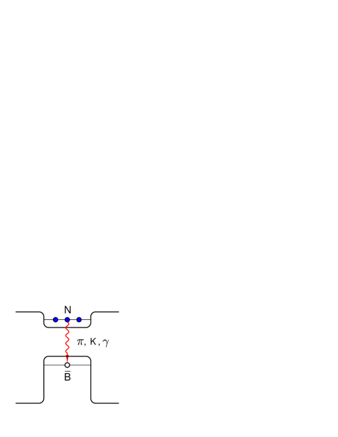
Figure 31: Annihilation of antibaryon–nuclear system as a ”super–transition” between the Fermi and Dirac seas.

As pointed out earlier, high–energy antiprotons have a better chance to penetrate deep into the nucleus. Under certain conditions discussed earlier they can be trapped into a deep bound state. We have demonstrated in Sect. V that the annihilation can be delayed in this case due to the reduction of energy released in this process. An antibaryon sitting in the nucleus can be viewed as a hole in otherwise filled Dirac sea. This state represents a strong excitation of the nucleus which soon or later will decay. Among other decay modes the most interesting is a super-transition when a nucleon from a discrete level of the Fermi sea jumps into the hole state in the Dirac sea. This can be achieved by emitting a single photon, pion or kaon with energy of about $Q=E_{N}+E_{\overline{B}}$ and isotropic angular distribution in the nucleus rest frame. Such process is forbidden in vacuum by the energy–momentum conservation laws. But in the considered case the recoil momentum can be carried away by the residual nucleus. This is analogous to the Pontecorvo–like reactions discussed in Sect. V. This process is illustrated in Fig. 31. The appearance of relatively narrow lines with energies of about $0.5-1$ GeV and width $\Delta E\simeq 20\div 50$ MeV in the spectrum of secondary photons or mesons would be a direct signature of the deeply–bound antibaryon–nuclear states.

VII.3 Explosive multifragmentation

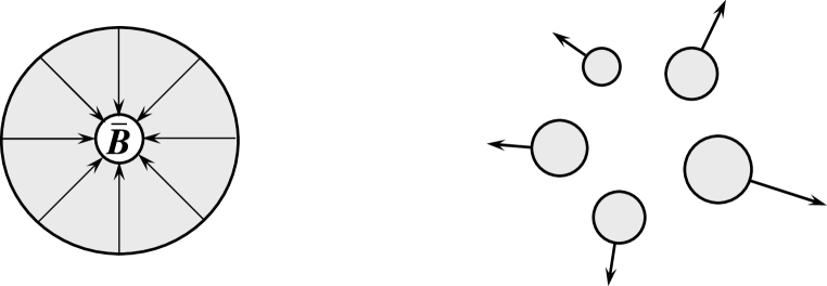
Figure 32: Multifragmentation (right) of a nuclear remnant formed after the antibaryon annihilation in a bound $\overline{B}$–nuclear system (left).

Another signal may come from the explosive disintegration of a compressed nucleus after the antibaryon annihilation. When the driving force for the compression disappears, the nucleus will expand as a compressed spring. As a result of the collective expansion the nucleus will be torn apart into fragments, as illustrated in Fig. 32. This process can be observed by measuring collective velocities of these fragments. Multifragmentation of nuclei induced by high–energy antiprotons has been studied earlier Bea99 , but with limited statistics. So far only minimum bias events have been analyzed. In this case the distribution of fragments follows closely predictions of the statistical multifragmentation model Bon95 where no collective effects are included. We emphasize again that a dedicated study with proper triggering is needed to find explosive events. Modern experimental technics allow to unambiguously distinguish between purely thermal and flow–driven multifragmentation.

VII.4 Multi–quark–antiquark clusters

It is interesting to look at the antibaryon–nuclear systems from a somewhat different point of view. An antibaryon implanted into a nucleus acts as a strong attracting center for nearby nucleons. Due to uncompensated attractive force these nucleons acquire acceleration towards the center. As the result of this inward collective motion the nucleons will pile up and produce a compression zone around the antibaryon. If such a process were completely elastic, it would look like a monopole–type oscillations around the equilibrium configuration found by solving static equations (see Sect. IV). In this dynamical process even stronger compression can be reached as compared with the one predicted by this static configuration. The maximum compression is achieved when the initial potential energy generated by the antibaryon is transformed into the compressional energy. Simple estimates show that local baryon densities up to $5\rho_{0}$ may be obtained in this way.

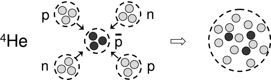
Figure 33: Schematic picture of deconfined quark–antiquark droplet formed in interaction of an antiproton with the ⁴He nucleus.

It is most likely that the deconfinement transition will occur at this stage and a high–density cloud containing an antibaryon and a few nucleons will appear in the form of a multi–quark–antiquark cluster. One may speculate that the whole ⁴He or even ¹⁶O nucleus can be transformed into the quark phase by this mechanism. This process is illustrated in Fig. 33.

As shown in Refs. Mis99 ; Mis00 and shortly discussed in Sect. III (see Fig. 4), an admixture of antiquarks to cold quark matter is energetically favorable. The problem of annihilation is now transferred to the quark level. But the argument concerning the reduction of available phase space due to the entrance–channel nuclear effects should work in this case too. Thus one may hope to produce relatively cold droplets of the quark phase by the inertial compression of nuclear matter initiated by an antibaryon. A similar mechanism for producing large quark bags was proposed in Ref. Raf80 . There the idea was that the annihilation fireball moving through the nucleus can grow by absorbing nucleons on its way.

Thus, the annihilation process in nuclear environment may serve as a breeder for creating new multi–quark–antiquark structures. We believe that among the decay modes of multi–quark–antiquark systems, like the one depicted in Fig. 33, not only usual hadrons, but also exotic states such as pentaquarks ($uudd\overline{d},uudd\overline{s},\ldots$) or heptaquarks ($uuu\overline{u}dd\overline{d},uu\overline{u}dd\overline{d},\ldots$) can be present. Moreover, more exotic states like baryonium ($3q\hskip 1.0pt3\overline{q}$), deutronium ($6q\hskip 1.0pt3\overline{q}$), tritonium ($9q\hskip 1.0pt3\overline{q}$) and even helionium ($12q\hskip 1.0pt3\overline{q}$ , see Fig. 33) can also be searched for. Discovery of such states would significantly extend our knowledge about the quark–gluon structure of matter. Such a study will be complimentary to the active search for exotic multi–quark systems stimulated by the discovery of the pentaquark Nak03 .

VIII Summary and discussion

In this paper we have demonstrated that antibaryons are of significant interest for nuclear physics. They can provide new and important information about the nature of strong interactions and structure of the vacuum. As well known, the relativistic nuclear models predict deep antibaryon potentials in nuclei generated by coherent action of mean scalar and vector fields. To verify this picture we study a real antibaryon bound in the nucleus instead of considering filled states of the Dirac sea. On the basis of the RMF model we performed detailed calculations of such bound antibaryon–nuclear systems taking into account the rearrangement of nuclear structure due to the presence of antibaryons. The self–consistent calculations lead to stronger bindings as compared to previous studies where the rearrangement effects were ignored. What is even more important, our calculations predict strong local compression of nuclei induced by the antibaryon. This opens a principal possibility of producing relatively cold and compressed nuclear matter in the laboratory. In contrast, in high-energy nuclear collisions the compression is always accompanied by a strong heating of nuclear matter.

Our second goal in this paper was to deceive a common delusion that the antibaryon annihilation in nuclei is so strong that it will shadow all other processes. We have performed detailed calculations assuming that annihilation rates into different exclusive channels are proportional to the available phase space. Due to reduced effective masses and (partial) cancelation of vector potentials, the energy available for annihilation of slow antibaryons (the reaction Q–value) is significantly reduced as compared to the minimum vacuum value, $m_{N}+m_{\overline{B}}$. Then many channels of in–medium annihilations are simply closed. This may lead to a dramatic reduction, by factors 5$\div$20, of the total annihilation rate. We estimate life times of deeply-bound antibaryon-nuclear systems on the level of 2$\div$20 fm/c that makes their observation feasible. This large margin in the life times is mainly caused by uncertainties in antibaryon coupling constants as well as the overlap integrals between the antibaryon and nucleon scalar densities. We have also analyzed multi–nucleon annihilation channels (Pontecorvo-like reactions) and found their contribution to be less than 40% of the single–nucleon annihilation.

We believe that bound antibaryon-nuclear systems can be produced by using antiproton beams of multi–GeV energy, e.g. at the future GSI facility. Since the annihilation cross section drops significantly with energy, a high–energy antiproton can penetrate deeper into the nuclear interior. Then it can be stopped there in an inelastic collision with a nucleon, e.g. via the reaction $A\hskip 1.0pt(\overline{p},N\pi)\hskip 1.0pt_{\overline{p}}\hskip 1.0ptA^{\prime}$, leading to the formation of a $\overline{p}$–doped nucleus. Reactions like $A\hskip 1.0pt(\overline{p},N\hskip 1.0pt\overline{K})\hskip 1.0pt_{\overline{\Lambda}}A^{\prime}$  and $A\hskip 1.0pt(\overline{p},\Lambda\pi)\hskip 1.0pt_{\overline{\Lambda}}A^{\prime}$ can be used to produce a $\overline{\Lambda}$–doped nucleus. Fast mesons, nucleons or lambdas can be used for triggering such events. Our estimates of the formation probability in a central $\overline{p}A$ collision give the values $10^{-5}-10^{-6}$. With the antiproton beam luminosity of 10³² cm${}^{-2}\,$s^-1 planned at GSI this will correspond to the reaction rate from tens to hundreds of desired events per second.

We have proposed several observable signatures which can be used for detection of antibaryon–nuclear bound states. They include exotic annihilation channels with emission of a single photon, pion or kaon; explosive multifragmentation of nuclei, and formation of multi–quark–antiquark clusters. The possibility of using antibaryon annihilation in nuclei to produce droplets of relatively cold quark matter is interesting by its own. This mechanism will work irrespective to the existence of antibaryon–nuclear bound states.

There remain many problems to be studied. The list of most urgent questions includes:

$\bullet$	how G–parity works in a many–body system and what are the antibaryon couplings
	to the meson fields?
$\bullet$	what is the role of exchange terms and dispersive corrections?
$\bullet$	how large is the unphysical self–interaction of antibaryons within the RMF approach?
$\bullet$	how to extend the RMF approach to include self–consistently imaginary contribution
	to the antibaryon self energy?
$\bullet$	how accurate are quasiclassical estimates of life times of bound antibaryon–nuclear
	systems?
$\bullet$	how these life times are affected by in–medium modifications of secondary mesons?

In addition, the nuclear rearrangement dynamics after the antibaryon capture should be studied on the basis of a dynamical approach like the TDHF model. Transport calculations of $\overline{p}A$ reactions are needed to check our simple estimates of the formation probabilities and annihilation rates. We are planning to address these questions in the future work.

Our most general conclusion is that the antibaryon–nuclear physics is a broad field of research which is not yet explored sufficiently well. It may bring about new interesting phenomena ranging from unusual annihilation channels to exotic antibaryon–nuclear or multi-quark-antiquark bound states. This is a nonperturbative domain of strong interactions and therefore the progress in this field can be achieved only by close cooperation of theory and experiment.

- (1) T. Walcher, Annu. Rev. Nucl. Part. Sci. 38, 67 (1989).
- (2) C. Amsler, Annu. Rev. Nucl. Part. Sci. 41, 219 (1991).
- (3) E. Klempt, F. Bradamante, A. Martin, and J.-M. Richard, Phys. Rep. 368, 119 (2002).
- (4) J.Z. Bai and BES Collaboration, Phys. Rev. Lett. 91, 022001 (2003).
- (5) C.Y. Wong, A.K. Kerman, G.R. Sachler, and A.D. Mackellar, Phys. Rev. C 29, 574 (1984).
- (6) C.J. Batty, E. Friedman, and A. Gal, Phys. Rep. 287, 385 (1997).
- (7) E.H. Auerbach, C.B. Dover, and S.H. Kahana, Phys. Rev. Lett. 46, 702 (1981).
- (8) H. Heiselberg, A.S. Jensen, A. Miranda, and G.C. Oades, Phys. Lett. B132, 279 (1983).
- (9) A.J. Baltz, C.B. Dover, M.E. Sainio, A. Gal, and G. Toker, Phys. Rev. C 32 1272 (1985).
- (10) J. Boguta, Phys. Lett. 106B, 245 (1981).
- (11) A. Bouyssy and S. Marcos, Phys. Lett. 114B, 397 (1982).
- (12) H.P. Duerr and E. Teller, Phys. Rev. 101, 494 (1956).
- (13) J.D. Walecka, Ann. Phys. 83, 491 (1974).
- (14) N. Auerbach, A.S. Goldhaber, M.B. Johnson, L.D. Miller, and A. Picklesimer, Phys. Lett. B182, 221 (1986).
- (15) G. Mao, H. Stöcker, and W. Greiner, Int. J. Mod. Phys. E8, 389 (1999).
- (16) I.N. Mishustin, Sov. J. Nucl. Phys. 52, 1135 (1990).
- (17) I.N. Mishustin, L.M. Satarov, J. Schaffner, H. Stöcker, and W. Greiner, J. Phys. G: Nucl. Part. Phys. 19, 1303 (1993).
- (18) R. Hofmann, A. Faessler, and T. Gutsche, J. Phys. G: Nucl. Part. Phys. 25, 1043 (1999).
- (19) J. Schaffner, I.N. Mishustin, L.M. Satarov, H. Stöcker, and W. Greiner, Z. Phys. A341, 47 (1991).
- (20) S. Teis, W. Cassing, T. Maruyama, and U. Mosel, Phys. Rev. C 50, 388 (1994).
- (21) A. Sibirtsev, W. Cassing, G.I. Lykasov, and M.V. Rzyanin, Nucl. Phys. A632, 131 (1998).
- (22) B.D. Serot and J.D. Walecka, Adv. Nucl. Phys. 16, 1 (1985).
- (23) P.G. Reinhard, Rep. Prog. Phys. 52, 439 (1989).
- (24) T. Bürvenich, I. N. Mishustin, L. M. Satarov, J. A. Maruhn, H. Stöcker, and W. Greiner, Phys. Lett. B 542, 261 (2002).
- (25) R.J. Furnstahl, J. Piewkarewicz, and B.D. Serot, nucl–th/0205048.
- (26) G. Lalazissis, J. König, and P. Ring, Phys. Rev. C 55, 540 (1997).
- (27) M. Rufa, P.–G. Reinhard, J.A. Maruhn, W. Greiner, and M. R. Strayer, Phys. Rev. C 38, 390 (1988).
- (28) M. Bender, K. Rutz, P.–G. Reinhard, J.A. Maruhn, and W. Greiner, Phys. Rev. C 60, 34304 (1999).
- (29) Y. Sugahara and H. Toki, Nucl. Phys. A579, 557 (1994).
- (30) W. Greiner and B. Müller, Quantum Mechanics: Symmetries (Springer, 2001).
- (31) K. Soutome, T. Maryama, and K. Saito, Nucl. Phys. A507, 731 (1990).
- (32) P.–G. Reinhard and R. Y. Cusson, Nucl. Phys. A378, 418 (1982).
- (33) I.N. Mishustin, L.M. Satarov, H. Stöcker, and W. Greiner, Phys. Rev. C 59, 3343 (1999).
- (34) I.N. Mishustin, L.M. Satarov, H. Stöcker, and W. Greiner, Phys. Rev. C 62, 034901 (2000).
- (35) W.W. Buck and D. Strottman, LANL report LA-UR-79-397, 1979.
- (36) J. Schaffner and I.N. Mishustin, Phys. Rev. C 53, 1416 (1996).
- (37) Y. Akaishi and T. Yamazaki, Phys. Rev. C 65, 044005 (2002).
- (38) S.-G. Zhou, J. Menq, and P. Ring, Phys. Rev. Lett. 91, 262501 (2003).
- (39) C.B. Dover, T. Gutsche, M. Maryama, and A. Faessler, Prog. Part. Nucl. Phys. 29, 87 (1992).
- (40) L.D. Landau and E.M. Lifshitz, Quantum Mechanics (Pergamon Press, Oxford, 1977).
- (41) G. Backenstoss et al., Nucl. Phys. B228, 424 (1983).
- (42) J. Sedlák and V. imák, Fiz. Elem. Chastits. At. Yadra 19, 445 (1988); [Sov. J. Part. Nucl. 19, 191 (1988)].
- (43) OBELIX Collab., Nucl. Phys. B (Proc. Suppl.) 56A, 58 (1997).
- (44) Crystal Barrel Collab., Phys. Lett. B322, 431 (1994).
- (45) Crystal Barrel Collab., Phys. Lett. B380, 453 (1996).
- (46) C. Amsler, Rev. Mod. Phys. 70, 1293 (1998).
- (47) Crystal Barrel Collab., Nucl. Phys. A720, 357 (2003).
- (48) Particle Data Group, K. Hagivara et. al., Phys. Rev. D 66, 010001 (2002).
- (49) A.B. Migdal, O.A. Markin, and I.N. Mishustin, Zh. Eksp. Teor. Fiz. 66, 443 (1974) [Sov. Phys.–JETP 39, 212 (1974)].
- (50) A.B. Migdal, E.E. Saperstein, M.A. Troitsky, and D.N. Voskresensky, Phys. Rep. 192, 179 (1990).
- (51) J. Wambach, Prog. Part. Nucl. Phys. 50, 615 (2003).
- (52) W. Cassing, Nucl. Phys. A700, 618 (2002).
- (53) P. Braun-Munzinger, J. Stachel, and C. Wetterich, nucl-th/0311005.
- (54) S. Gjesdal et al., Phys. Lett. 40B, 152 (1972).
- (55) F. Eisele et al., Phys. Lett. 60B, 297 (1976).
- (56) J.P. Bondorf, A.S. Botvina, A.S Iljinov, I.N. Mishustin, and K. Sneppen, Phys. Rep. 257, 133 (1995).
- (57) B.M. Pontecorvo, Zh. Eksp. Teor. Fiz. 30, 947 (1956) [Sov. Phys.–JETP 3, 966 (1957)].
- (58) J. Rafelski, Phys. Lett. 91B, 281 (1980).
- (59) W. Weise, Nucl. Phys. A558, 219c (1993).
- (60) OBELIX Collab., Nucl. Phys. A700, 159 (1997).
- (61) S. Banerjee, S. Ganguli, P.K. Malhotra, and R. Raghavan, Nucl. Phys. B150, 119 (1979).
- (62) B. Jakobsson et al., Phys. Rev. Lett. 78, 3828 (1997).
- (63) GSI Future Project, see http://www-new.gsi.de/zukunftsprojekt/index_e.html.
- (64) W. Scheid, H. Müller, and W. Greiner, Phys. Rev. Lett. 32, 741 (1974).
- (65) L. Beaulieu et al., Phys. Lett. B463, 159 (1999).
- (66) T. Nakano et al., Phys. Rev. Lett. 91, 012002 (2003).