Abstract

We study Compton scattering in systems with A=1 and 2 using chiral perturbation theory up to fourth order. For the proton we fit the two undetermined parameters in the $O(Q^{4})$ $\gamma$p amplitude of McGovern to experimental data in the region $\omega,\sqrt{|t|}\leq 180$ MeV, obtaining a $\chi^{2}/{\rm d.o.f.}$ of 133/113. This yields a model-independent extraction of proton polarizabilities based solely on low-energy data: $\alpha_{p}=(12.1\pm 1.1~{}({\rm stat.}))_{-0.5}^{+0.5}~{}({\rm theory})$ and $\beta_{p}=(3.4\pm 1.1~{}({\rm stat.}))_{-0.1}^{+0.1}~{}({\rm theory})$, both in units of $10^{-4}~{}{\rm fm}^{3}$. We also compute Compton scattering on deuterium to $O(Q^{4})$. The $\gamma$d amplitude is a sum of one- and two-nucleon mechanisms, and contains two undetermined parameters, which are related to the isoscalar nucleon polarizabilities. We fit data points from three recent $\gamma$d scattering experiments with a $\chi^{2}/{\rm d.o.f.}=26.6/20$, and find $\alpha_{N}=(13.0\pm 1.9~{}({\rm stat.}))_{-1.5}^{+3.9}~{}({\rm theory})$ and a $\beta_{N}$ that is consistent with zero within sizeable error bars.

PACS nos.: 13.60.Fz, 12.39.Fe, 25.20.-x, 12.39.Pn, 21.45.+v

1 Introduction

Compton scattering on the proton, neutron, and deuteron provides a window on the internal dynamics of these strongly-interacting systems. As this is an electromagnetic process, the photon-target interaction can be treated using well-controlled approximations. At the same time Compton scattering is governed by a different set of target structure functions than, say, electron scattering, and so probes complementary aspects of the strong nuclear force. For example, in the case of the proton, quark models indicate that even at quite low energies $\gamma$p scattering can reveal distinctive information about the charge and current distributions produced by the nucleon’s quark substructure [1, 2].

The deuteron represents a different theoretical challenge. Its structure is governed by the nucleon-nucleon ($NN$) interaction. A number of models of this interaction exist which very accurately describe experimental data on $NN$ scattering at laboratory energies below 350 MeV. However, these successful approaches differ significantly in their underlying assumptions. They range from models which are almost purely phenomenological [3] to multi-boson-exchange models [4, 5, 6] that make detailed assumptions about how QCD plays out in the $NN$ system, e. g. the role of the pomeron [5, 6]. Clearly, $NN$ scattering alone cannot completely constrain the form of strong interactions at low energies. Deuteron Compton scattering is a way of probing the deuteron bound-state dynamics generated by different models. Furthermore, any theoretical treatment of this reaction must incorporate not just photon interactions with the target via the one-body Compton process but two-body mechanisms as well: the input to a calculation of the $\gamma$d amplitude includes the $\gamma N$ amplitude plus Compton-scattering two-body currents. These two-body currents should be constructed in a way that is consistent with both the single-nucleon Compton dynamics and the $NN$ potential used to generate the nuclear bound state.

Over the last several years a framework [7] based on effective field theory (EFT) [8] has been developed that allows such consistency. Importantly, EFTs also satisfy the symmetry constraints of QCD while making only minimal theoretical assumptions. This framework can be applied to the Compton processes we are interested in, provided that the photon energy is well below the chiral symmetry breaking scale, $\Lambda_{\chi}\sim 4\pi f_{\pi}\sim M\sim{m_{\rho}}$. In this regime photon-nucleon and photon-deuteron scattering are governed by the approximate chiral $SU(2)_{L}\times SU(2)_{R}$ symmetry of QCD. The spontaneous breaking of this symmetry to isospin $SU(2)_{V}$ results in the existence of three Goldstone bosons, which are identified with the pions ($\pi^{+}$, $\pi^{-}$, and $\pi^{0}$).

An EFT can be built from the most general Lagrangian involving pions and nucleons  which is constrained only by approximate chiral symmetry and the relevant space-time symmetries. In this EFT, known as chiral perturbation theory ($\chi$PT), pions interact through vertices with a countable number of derivatives and/or insertions of the quark mass matrix. Therefore $S$-matrix elements can be expressed as simultaneous expansions in powers of momenta and pion masses over the characteristic scale of physics that is not included explicitly in the EFT, $\Lambda_{\chi}$. A generic amplitude can be written as:

$$T=C(\Lambda_{\chi})\,\sum_{\nu}\,\left(\frac{Q}{\Lambda_{\chi}}\right)^{\nu}{\cal F}_{\nu}(Q/m_{\pi}),$$ (1)

where $Q$ represents the external momenta and/or the pion mass, ${\cal F}_{\nu}$ is a calculable function with ${\cal F}_{\nu}(1)$ of order one, $C$ is an overall normalization factor, and $\nu$ is a counting index.

$\chi$PT has proven remarkably successful, with a number of single-nucleon processes [9]—including $\gamma$p scattering [10, 11, 12]—now computed to several nontrivial orders. In $\chi$PT, as in any EFT, the price to be paid for the absence of model assumptions is a lack of detailed information about physics at distance scales much shorter than the wavelength of the probe. This price translates into the presence in $\chi$PT amplitudes of certain undetermined interaction strengths, or “low-energy constants” (LECs). These constants can be estimated using models of the short-distance physics, but in the purest form of $\chi$PT they should be fitted to experimental data.

There has been intense recent effort dedicated to extending $\chi$PT to processes with more than a single nucleon [7]. The fundamental difficulty in making this extension is the treatment of the effects of nuclear binding. At momenta comparable to the pion mass the few-nucleon EFT first proposed by Weinberg [13] still provides a paradigm for the application of EFT to nuclear systems. Use of this few-nucleon EFT has developed to the point where computations of processes involving two nucleons with any number of pions and photons can be carried out at levels of precision comparable to those achieved using $\chi$PT in the single-nucleon sector [14]. The present paper is part of this ongoing program [15, 16].

During roughly the same period over which EFT has developed as a tool for analyzing low-energy QCD dynamics, experimental facilities with tagged photons have made possible a new generation of Compton scattering experiments which probe the low-energy structure of nucleons and nuclei. An extensive database now exists for Compton scattering on the proton at photon energies below 200 MeV [17], with this database being considerably enhanced by the recent data taken in the TAPS setup at MAMI by Olmos de Léon et al. [18]. In the nuclear case the past decade has seen a set of experiments that establish—for the first time—a modern data set for Compton scattering on the deuteron. Data now exist for coherent $\gamma d\rightarrow\gamma d$ from 49 to 95 MeV [19, 20, 21], and for quasi-free $\gamma d\rightarrow\gamma pn$ from 200 to 400 MeV [22, 23, 24].

These experimental and theoretical developments come together in studies of Compton scattering on the $A=1$ and $A=2$ system in $\chi$PT. Nucleon Compton scattering has been studied in $\chi$PT to $O(Q^{3})$ [9, 10] and $O(Q^{4})$ [11, 12]. To $O(Q^{3})$, there are no undetermined parameters in the $\gamma$p amplitude, so $\chi$PT makes predictions for $\gamma$p scattering. These agree reasonably well with low-energy differential cross-section data [9, 25]. At the next order in the chiral expansion, $O(Q^{4})$, there are four undetermined parameters, two for $\gamma$p scattering and two for $\gamma$n scattering. These counterterms account for short-range contributions to nucleon structure. Minimally one needs four pieces of experimental data to determine their values, and once they are fixed $\chi$PT  makes improved, model-independent predictions for Compton scattering on protons and neutrons [12]. Below we use low-energy proton data in order to obtain the two short-distance parameters associated with the proton, and so make a completely model-independent determination of the $\chi$PT $\gamma$p amplitude up to fourth order in small quantities.

In the $A=2$ system, the amplitude for coherent Compton scattering on the deuteron was computed to $O(Q^{3})$ in Ref. [15]. There are no free parameters at this order. The corresponding cross section is in good agreement with the Illinois data [19] at 49 and 69 MeV, but underpredicts the SAL data [20] at 95 MeV. The calculation of Ref. [15] also yields cross sections which agree well with the more recent Lund data [21]. In the present paper we extend this calculation to $O(Q^{4})$. At this order coherent $\gamma$d scattering is sensitive to two isoscalar combinations of the four free parameters in the $O(Q^{4})$ $\gamma N$ amplitude. We will show that fitting these two parameters to experiment yields $\gamma$d cross sections which are in good agreement with the existing data for momentum transfers and photon energies below 160 MeV. A summary of earlier $O(Q^{4})$ $\chi$PT results for both $\gamma$p and $\gamma$d scattering was presented in Ref. [16]. The current paper contains a considerably more detailed discussion. Because of errors in the fits to $\gamma$d data reported in Ref. [16] the central values found here for the isoscalar polarizabilities differ significantly from those given in Ref. [16] (see Section 6.4 for a full explanation).

Very low-energy nucleon Compton scattering (with $\omega$ significantly below $m_{\pi}$) has been a focus of particular theoretical interest. At these energies, the $\chi$PT $\gamma N$ amplitude can be expanded in powers of $\omega/m_{\pi}$. This yields a $T$-matrix that is a simple power series in $\omega$, with coefficients which are functions of $\chi$PT parameters. In the nucleon rest frame,

$$T={\vec{\epsilon}\,^{\prime}}\cdot{\vec{\epsilon}}\left(-\frac{{\cal Z}^{2}e^{2}}{M}+4\pi\alpha\omega\omega^{\prime}\right)+4\pi\beta\,{\vec{\epsilon}\,^{\prime}}\times\vec{k}^{\prime}\cdot{\vec{\epsilon}}\times\vec{k}+\ldots.$$ (2)

Here the ellipses represent higher powers of energy and momentum as well as relativistic corrections, and ${\vec{\epsilon}}$ (${\vec{\epsilon}\,^{\prime}}$) is the polarization vector of the initial- (final-) state photon and $\vec{k}$ (${{\vec{k}}^{\,\prime}}$) is its three-momentum. The first term in this series is a consequence of gauge invariance, and is the Thomson limit for Compton scattering on a target of mass $M$ and charge ${\cal Z}|e|$. Meanwhile, the coefficients of the second and third terms are the nucleon electric and magnetic polarizabilities, $\alpha$ and $\beta$. To $O(Q^{3})$ in $\chi$PT they are completely given by pion-loop effects [10]:

$$\alpha_{p}=\alpha_{n}=\frac{5e^{2}g_{A}^{2}}{384\pi^{2}f_{\pi}^{2}m_{\pi}} = 12.2\times 10^{-4}\,{\rm fm}^{3};$$

$$\beta_{p}=\beta_{n}=\frac{e^{2}g_{A}^{2}}{768\pi^{2}f_{\pi}^{2}m_{\pi}} = 1.2\times 10^{-4}\,{\rm fm}^{3},$$ (3)

with $g_{A}$ the axial coupling of the nucleon and $f_{\pi}$ the pion decay constant. We emphasize that the polarizabilities are predictions of $\chi$PT at this order: they diverge in the chiral limit because they arise from pion-loop effects. In less precise language, $\chi$PT tells us that polarizabilities are dominated by the dynamics of the long-range pion cloud surrounding the nucleon, rather than by short-range dynamics, and thus should provide a sensitive test of chiral dynamics.

At $O(Q^{4})$ the four undetermined parameters alluded to above contribute to the polarizabilities [11]. They can be understood as representing short-distance ($r\ll 1/m_{\pi}$) effects in $\alpha$ and $\beta$. The results from our fits to proton Compton data provide the first completely model-independent determination of proton polarizabilities. These results, together with an analysis of various remaining sources of theoretical uncertainty, are given in Section 4 below.

While data from Compton scattering on hydrogen targets can be used to extract the proton polarizabilities $\alpha_{p}$ and $\beta_{p}$, the absence of dense, stable, free neutron targets requires that the neutron polarizabilities $\alpha_{n}$ and $\beta_{n}$ be extracted from scattering on deuterium (or some other nuclear target). Coherent Compton scattering on deuterium depends on the polarizability combinations $\alpha_{N}\equiv(\alpha_{p}+\alpha_{n})/2$ and $\beta_{N}\equiv(\beta_{p}+\beta_{n})/2$ through interference between the polarizability pieces of the $\gamma N$ amplitude and the proton Thomson term. Thus $\alpha_{N}$ and $\beta_{N}$ can be extracted from nuclear data, but to do so requires a consistent theoretical framework that cleanly separates single-nucleon properties from multi-nucleon effects. In the long-wavelength limit pertinent to polarizabilities EFT provides a model-independent way to do exactly this [7, 8, 9], and thus we would argue that $\chi$PT (or at least some systematic EFT) is an essential tool in the quest to obtain $\alpha_{N}$ and $\beta_{N}$ from deuteron Compton data. Our $\chi$PT analysis of $\gamma$d data in Section 6 facilitates a model-independent extraction of $\alpha_{N}$ and $\beta_{N}$, as well as a quantitative assessment of the uncertainty associated with the freedom to choose different $NN$ potentials when generating the deuteron bound state.

Our results for both $\gamma$d cross sections and extracted values of $\alpha_{N}$ and $\beta_{N}$ agree qualitatively with potential-model treatments of $\gamma$d scattering at these energies [26, 27, 28]. The different potential-model calculations all yield similar results if similar input is supplied—in particular in the form of comprehensive meson-exchange currents. Typically though, the one- and two-nucleon Compton scattering mechanisms in potential models are not derived in a mutually-consistent fashion. The calculations of Refs. [26, 27, 28] also tend to incorporate significantly more model assumptions about short-distance physics than are necessary in an EFT approach.

We note that calculations of Compton scattering on the deuteron in EFTs other than the one employed here exist in the literature. For example, in Ref. [29], an EFT where pions are integrated out is employed. This EFT is under good theoretical control and is a very precise computational tool, but it is limited in its utility to momenta well below the pion mass. In Ref. [30] a different power counting [31] from ours was used in which pion exchange is treated in perturbation theory. While this power counting is well-adapted to processes at momenta below the pion mass, it is now known to break down at quite low energies [32].

The rest of the paper is structured as follows. In Section 2 we summarize those aspects of $\chi$PT which are directly relevant to our calculation, including the power-counting scheme and the pertinent terms in the chiral Lagrangian. In Section 3 we explain how this theory is applied to Compton scattering on the proton up to $O(Q^{4})$, reviewing the results of Ref. [12]. In Section 4 we fit the two unknown parameters in the $O(Q^{4})$ $\chi$PT $\gamma$p amplitude to $\gamma$p scattering data with $\omega,\sqrt{|t|}\leq 180$ MeV. In Section 5 we turn to the A=2 system, computing the Feynman amplitudes that contribute to photon scattering on the two-nucleon system at $O(Q^{4})$. In Section 6 we present results for differential cross sections for Compton scattering on unpolarized deuteron targets. We discuss higher-order effects and the extent to which a determination of neutron polarizabilities from elastic $\gamma$d is possible. Finally, in Section 7 we summarize our work, and identify future directions for the theoretical study of this reaction.

2 Baryon Chiral Perturbation Theory

In this section we briefly discuss the effective chiral Lagrangian underlying our calculations and the corresponding power counting.

2.1 Effective Lagrangian

QCD has an approximate chiral $SU(2)_{L}\times SU(2)_{R}$ symmetry that is spontaneously broken at a scale $\Lambda_{\chi}\sim 1$ GeV. Below this scale there are no obvious small coupling constants in which to expand. Effective field theory is the technique by which a hierarchy of scales is developed into a perturbative expansion of physical observables. Here we are interested in processes where the typical momenta of all external particles is $p\ll\Lambda_{\chi}$, so we identify our expansion parameter as $p/\Lambda_{\chi}$.

In a system with broken symmetries this technique is especially powerful. When a continuous symmetry is spontaneously broken there are always massless Goldstone modes which dominate the low-energy dynamics. If the chiral symmetry of QCD were exact, $p/\Lambda_{\chi}$ would be the only expansion parameter. However, in QCD $SU(2)_{L}\times SU(2)_{R}$ is softly broken by the small quark masses. This explicit breaking implies that the pion has a small mass in the low-energy theory. Since ${m_{\pi}}/\Lambda_{\chi}$ is then also a small parameter, we have a dual expansion in $p/\Lambda_{\chi}$ and ${m_{\pi}}/\Lambda_{\chi}$.

We will limit ourselves to the region where $m_{\pi}\sim p<M_{\Delta}-M$. ($M$ and $M_{\Delta}$ stand for the nucleon and Delta-isobar mass, respectively.) In this regime we can keep only pions and nucleons as active degrees of freedom, and the low-energy EFT is $\chi$PT without an explicit Delta-isobar field. We take $Q$ to represent either a small momentum or a pion mass, and seek an expansion in powers of $Q/\Lambda_{\chi}$. We implicitly include the mass scale of the degrees of freedom that have been integrated out—$M_{\Delta}-M$, $m_{\rho}$, etc.— in $\Lambda_{\chi}$. One might reasonably expect that the convergence of the theory will improve upon the inclusion of an explicit Delta field [33, 34]. Work on nucleon Compton scattering along these lines is ongoing [35, 36].

Although chiral symmetry is no longer a symmetry of the vacuum, it remains a symmetry of the Lagrangian. One can show [37] that a choice of pion fields is possible, in which all pion interactions are either derivative or proportional to $m_{\pi}^{2}$. The symmetries of QCD still permit an infinite number of such interactions though, and so it is necessary to order the strong interactions according to the so-called index of the interaction [13]. For an interaction labeled $i$ this is defined by:

$${\Delta_{i}}\equiv{d_{i}}+{f_{i}}/2-2$$ (4)

with $d_{i}$ the sum of the number of derivatives or powers of $m_{\pi}$ and $f_{i}$ the number of nucleon fields. Since pions couple to each other and to nucleons through either derivative interactions or quark masses, there is a lower bound on the index of the interaction: ${\Delta_{i}}\geq 0$. We write the effective Lagrangian as

$${\cal L}=\sum_{\Delta=0}^{\infty}{\cal L}^{(\Delta)}.$$ (5)

So far this only accounts for strong interactions. The electromagnetic field can enter ${\cal L}$ either through minimal substitution or by the addition of terms involving the electromagnetic field strength tensor. The former simply has the effect of replacing a derivative by a factor of the charge $e$. And in either case we now have another expansion: one in the small electromagnetic coupling $\alpha_{\rm em}=e^{2}/4\pi$. However, since we work only to leading order in this expansion it is convenient to enlarge the definition of $d_{i}$ so that it includes powers of $e$, and then continue to classify interactions according to the index $\Delta_{i}$ defined by Eq. (4).

The technology that goes into building an effective Lagrangian and extracting the Feynman rules is standard by now and presented in great detail in Ref. [9]. Here we list only the elements necessary for our calculations.

The pion triplet is contained in a matrix field

$$\Sigma=\xi^{2}\equiv\sqrt{1-\frac{\vec{\pi}^{2}}{f_{\pi}^{2}}}+i\frac{{\vec{\pi}}\cdot{\vec{\tau}}}{f_{\pi}},$$ (6)

where $f_{\pi}$ is the pion decay constant, for which we adopt the value $f_{\pi}=92.4$ MeV. Under $SU(2)_{L}\times SU(2)_{R}$, $\Sigma$ transforms as $\Sigma\rightarrow L\Sigma{R^{\dagger}}$ and $\xi$ as $\xi\rightarrow L\xi{U^{\dagger}}=U\xi{R^{\dagger}}$; here $L$($R$) is an element of $SU(2)_{L}$ ($SU(2)_{R}$), and $U$ is defined implicitly. It is convenient to assign the nucleon doublet $N$ the transformation property $N\rightarrow UN$. With ${\cal Z}=(1+{\tau_{3}})/2$ we can write the pion covariant derivative as

$${D_{\mu}}\Sigma={\partial_{\mu}}\Sigma-ie{{\cal A}_{\mu}}[{\cal Z},\Sigma].$$ (7)

Out of $\xi$ one can construct

$${V_{\mu}} = \frac{1}{2}[{\xi^{\dagger}}({\partial_{\mu}}-ie{{\cal A}_{\mu}}{\cal Z})\xi+\xi({\partial_{\mu}}-ie{{\cal A}_{\mu}}{\cal Z}){\xi^{\dagger}}]$$ (8)

$${A_{\mu}} = \frac{i}{2}[{\xi^{\dagger}}({\partial_{\mu}}-ie{{\cal A}_{\mu}}{\cal Z})\xi-\xi({\partial_{\mu}}-ie{{\cal A}_{\mu}}{\cal Z}){\xi^{\dagger}}],$$ (9)

which transform as ${V_{\mu}}\rightarrow U{V_{\mu}}{U^{\dagger}}+U{\partial_{\mu}}{U^{\dagger}}$ and ${A_{\mu}}\rightarrow U{A_{\mu}}{U^{\dagger}}$ under $SU(2)_{L}\times SU(2)_{R}$. $V_{\mu}$ is used to build covariant derivatives of the nucleon,

$$D_{\mu}N=({\partial_{\mu}}+{V_{\mu}})N.$$ (10)

(Ref. [38] uses $\Gamma_{\mu}$ where we have used $V_{\mu}$ and ${\textstyle{1\over 2}}u_{\mu}$ for our $A_{\mu}$.) The electromagnetic field enters not only through minimal coupling in the covariant derivatives, but also through

$$f_{\mu\nu}=e({\xi^{\dagger}}{\cal Z}\xi+\xi{\cal Z}{\xi^{\dagger}}){F_{\mu\nu}},$$ (11)

where ${F_{\mu\nu}}=\partial_{\mu}A_{\nu}-\partial_{\nu}A_{\mu}$ is the usual electromagnetic field strength tensor.

Because the nucleon mass is large, $M\gg Q$, it plays no dynamical role: nucleons are non-relativistic objects in the processes we are interested in. The field $N$ can be treated as a heavy field of velocity $v$ in which on-mass-shell propagation through $\exp(iM{v\cdot x})$ has been factored out. In the rest frame of the nucleon, the velocity vector ${v^{\mu}}=(1,\vec{0})$. The spin operator is denoted by $S^{\mu}$, and in the nucleon rest frame $S^{\mu}=(1/2)(0,\vec{\sigma})$. This formulation of $\chi$PT is sometimes called heavy-baryon chiral perturbation theory (HB$\chi$PT).

With these ingredients, it is straightforward to construct the effective Lagrangian. As will become clear later, in order to calculate Compton scattering to $O(Q^{4})$ we need to consider interactions with $\Delta_{i}\leq 3$.

The leading-order Lagrangian is

$${\cal L}^{(0)} = \frac{1}{4}{f_{\pi}^{2}}{\rm Tr}({D_{\mu}}{\Sigma^{\dagger}}{D^{\mu}}{\Sigma})+\frac{1}{4}{{f_{\pi}^{2}}{m_{\pi}^{2}}}{\rm Tr}({\Sigma}+{\Sigma^{\dagger}})$$ (12)

$$+iN^{\dagger}(v\cdot D)N+2g_{A}N^{\dagger}(A\cdot S)N$$

$$-\frac{C_{0}}{8}\left[3N^{\dagger}N\,N^{\dagger}N+N^{\dagger}SN\cdot N^{\dagger}SN\right]+\ldots$$

with $g_{A}=1.267$ the axial-vector coupling of the nucleon and $C_{0}$ a parameter determined from $NN$ scattering in the ³S₁ channel. The next-to-leading-order (NLO) terms are contained in

$${\cal L}^{(1)} = \frac{1}{2M}N^{\dagger}\left\{{-D^{2}}+(v\cdot D)^{2}+2i{g_{A}}\{{v\cdot A},{S\cdot D}\}\right.$$ (13)

$$-\frac{i}{2}[{S^{\mu}},{S^{\nu}}]\left[(1+{\kappa_{v}}){f_{\mu\nu}}+\frac{1}{2}({\kappa_{s}}-{\kappa_{v}}){\rm Tr}{f_{\mu\nu}}\right]$$

$$\left.+2Mc_{1}m_{\pi}^{2}{\rm Tr}({\Sigma}+{\Sigma^{\dagger}})+\left(8Mc_{2}-g_{A}^{2}\right)(v\cdot A)^{2}+8Mc_{3}A^{2}\right\}N+\ldots,$$

where ${\kappa_{v}}={\kappa_{p}}-{\kappa_{n}}$ and ${\kappa_{s}}={\kappa_{p}}+{\kappa_{n}}$ are parameters related to the anomalous magnetic moments of the proton, $\kappa_{p}=1.79$, and neutron, $\kappa_{n}=-1.91$; and $c_{1}$, $c_{2}$, and $c_{3}$ are parameters that can be determined from $\pi N$ scattering. We use $c_{1}=-0.81$ GeV^-1, $c_{2}=2.5$ GeV^-1, and $c_{3}=-3.8$ GeV^-1 [39] (compare with similar values obtained from $NN$ scattering [40]). The ellipses in Eq. (13) indicate that we have not written down pieces of ${\cal L}^{(1)}$ which are not relevant to our computation of $\gamma N$ and $\gamma$d scattering.

At sub-sub-leading order (N²LO):

$${\cal L}^{(2)} = -\frac{e^{2}}{32\pi^{2}f_{\pi}}\pi_{3}\epsilon^{\mu\nu\rho\sigma}F_{\mu\nu}F_{\rho\sigma}$$ (14)

$$-\frac{C_{2}}{8}\left[3N^{\dagger}N\,N^{\dagger}\left(-D^{2}+(v\cdot D)^{2}\right)N+N^{\dagger}SN\cdot N^{\dagger}S\left(-D^{2}+(v\cdot D)^{2}\right)N+h.c.\right]$$

$$-\frac{C_{\epsilon}}{2}\left[N^{\dagger}(S\cdot D)N\,N^{\dagger}(S\cdot D)N+h.c.\right]+\ldots$$

where the first term is from the chiral anomaly, with $\epsilon_{0123}=1$, and the other two terms are corrections to the two-nucleon potential in the deuteron channel, with the coefficients $C_{2}$ and $C_{\epsilon}$ determined by fits to $NN$ scattering data.

In Eq. (14) we do not explicitly display terms which are needed for our computation below and have coefficients that are determined by Lorentz invariance. These coefficients are dimensionless numbers times $1/M^{2}$, and the relevant numbers can be extracted from Ref. [38]. A fixed-coefficient $\gamma N$ seagull from ${\cal L}^{(2)}$ which enters the NLO $\gamma N$ amplitude stems from the 12th and 13th terms of Eq. (3.8) in Ref. [38], while the $\gamma NN$ pieces of ${\cal L}^{(2)}$ that contribute to $\gamma N$ scattering at N²LO can be obtained from the 5th, 9th, 12th and 13th terms of Eq (3.8) and the last term of Eq. (3.9) in that paper.

Finally, the relevant N³LO terms are given by

$${\cal L}^{(3)}=2\pi N^{\dagger}\left\{\left[\delta\beta_{N}+\delta\beta_{v}\tau_{3}\right]{\textstyle{1\over 2}}g_{\mu\nu}-\left[(\delta\alpha_{N}+\delta\beta_{N})+(\delta\alpha_{v}+\delta\beta_{v})\tau_{3}\right]v_{\mu}v_{\nu}\right\}F^{\mu\rho}F^{\nu}_{\;\;\rho}N+\ldots,$$ (15)

where $\delta\alpha_{N}$ ($\delta\beta_{N}$) and $\delta\alpha_{v}$ ($\delta\beta_{v}$) are short-range contributions to the isoscalar and isovector electric (magnetic) polarizabilities of the nucleon, $\delta\alpha_{p}=(\delta\alpha_{N}+\delta\alpha_{v})/2$ and $\delta\alpha_{n}=(\delta\alpha_{N}-\delta\alpha_{v})/2$ (similarly for $\delta\beta_{p}$ and $\delta\beta_{n}$), which we seek to determine. These LECs are linear combinations of $e_{89}$–$e_{94}$ of Fettes et al. [38]. The fixed-coefficient pieces of $e_{89}$–$e_{94}$ are given in Table 6 of that paper. Other relevant terms in ${\cal L}^{(3)}$ which have only fixed coefficients and are not written in Eq. (15) but can be found in Ref. [38] are $O_{117}$ and $O_{118}$ of Table 5, as well as $X_{41}$ and $X_{53}$ of Table 8 and $Y_{11}$ of Table 9.

2.2 Power counting

Scattering amplitudes are computed from Feynman diagrams built from the effective Lagrangian. Observables are then power series in momenta and pion masses, with the non-analyticities mandated by perturbative unitarity. The generic form for an amplitude is shown in Eq. (1).

Counting powers of $Q$ is simple, except for one important subtlety. The simple part is that each derivative or power of the pion mass at a vertex contributes $Q$ to the order of a diagram, each loop integral contributes $Q^{4}$, each delta function of four-momentum conservation contributes $Q^{-4}$, and each pion propagator contributes $Q^{-2}$. The complication arises from the fact that in multi-nucleon systems there exist intermediate states that differ in energy from the initial and final states by only the kinetic energy of nucleons, which is $O(Q^{2}/M)$. Diagrams in which such intermediate states appear are called reducible, while ones containing only intermediate states that differ in energy from initial/final states by an amount of $O(Q)$ are called irreducible.

First we consider only irreducible diagrams. By definition these are graphs in which the energies flowing through all internal lines are of $O(Q)$. A nucleon propagator then contributes $Q^{-1}$, and we find that a diagram with $A$ nucleons, $L$ loops, $C$ separately connected pieces, and $V_{i}$ vertices of type $i$ contributes $Q^{\nu}$, with [13, 41]

$$\nu=4-{A}-2C+2L+{\sum_{i}}{V_{i}}{\Delta_{i}}.$$ (16)

Eq. (1) follows immediately from the assumption that the parameters in the effective Lagrangian scale as numbers of $O(1)$ times the appropriate power of $\Lambda_{\chi}$. Hence the leading irreducible graphs are tree graphs ($L=0$) with the maximum number of separately connected pieces ($C=max$), and with leading-order ($\Delta_{i}=0$) vertices. Higher-order graphs (with larger powers of $\nu$) are perturbative corrections to this leading effect. In this way, a perturbative series is generated by increasing the number of loops $L$, decreasing the number of connected pieces $C$, and increasing the number of derivatives, pion masses and/or nucleon fields in interactions.

Processes involving one or zero nucleons and any number of light particles with $p\sim m_{\pi}$ only receive contributions from irreducible diagrams, and there is good evidence that the resulting $\chi$PT  power counting defined by Eq. (16) works in most kinematics (exceptions are possible, e.g., near threshold pion three-momenta may be smaller than the $\sim m_{\pi}$ assumed in deriving Eq. (16)) [9]. In processes involving more than one nucleon, the full amplitude consists of irreducible subdiagrams linked by reducible states. New divergences arise from these reducible intermediate states, which can potentially upset the scaling of the EFT parameters with $\Lambda_{\chi}$. Weinberg [13] has implicitly assumed that this is not the case, and thus that the $\chi$PT power counting continues to hold for irreducible diagrams.

It is now known that this assumption is not always correct [42]. In particular, consistency of renormalization in $NN$ scattering seems to require that some pion-mass contributions should be demoted to higher orders than in Weinberg’s original power counting. On the other hand, the error of not doing so is apparently numerically small [43]. This explains the phenomenological successes of applications of Weinberg’s proposal to few-nucleon systems [7, 41], including to $\gamma$d scattering [15] and a number of other reactions involving external probes of deuterium [14]. Here we continue to organize our calculation according to the power counting (16), but we will see some indications that the irreducible diagrams for Compton scattering on deuterium are not behaving exactly as Weinberg’s straightforward chiral power counting for them would suggest.

In an $A$-nucleon system which is not subject to any external probes, the sum of $A$-nucleon irreducible diagrams is, by definition, the potential $V$. To obtain the full two-nucleon Green’s function $G$, these irreducible graphs are iterated using the free two-nucleon Green’s function $G_{0}$, which can, of course, have a small energy denominator that does not obey the $\chi$PT power-counting: $G=G_{0}+G_{0}VG$. Making a spectral decomposition of $G$ we can extract the piece corresponding to the deuteron pole. Since $V$ is two-particle irreducible we may perform a chiral power counting on it as per Eq. (16). Such a potential was constructed including terms up to $\nu=3$ and with an explicit Delta field in Refs. [44]. Better fits have now been achieved using a potential without explicit Delta’s at $\nu=3$ [45, 46]. Recently the first calculation of $V$ to $\nu=4$ appeared, and a good fit to $NN$ scattering data for lab energies below 290 MeV resulted [47]. Here we use the wave function obtained from the NLO ($\nu=2$) potential of Ref. [45], as that is the consistent choice given the chiral order at which we calculate $\gamma$d scattering. Since this is only an NLO potential the quality of the fit to $NN$ scattering data is not nearly as good as that found in modern phenomenological potentials, or in Ref. [47]. In order to get a sense of how large the impact of higher-order terms in $V$ might be, we have also computed $\gamma$d scattering using deuteron wave functions generated from a modern one-boson-exchange $NN$ potential [5], and the Bonn OBEPQ [4].

When we consider external probes with momenta of order $Q$, the sum of irreducible diagrams forms a kernel $K$ for the process of interest, here the kernel $K_{\gamma\gamma}$ for $\gamma NN\rightarrow\gamma NN$. Again, the power counting of Eq. (16) applies to this object, since all two-nucleon propagators in it scale as $Q^{-1}$, as long as the photon energy $\omega\sim Q$. Note also that in order to have an irreducible graph in which two photons are attached to different nucleons the two nucleons must be connected by some interaction, so that there is a mechanism to carry the energy of order $Q$ from one nucleon to the other. Thus such graphs should be regarded as having one separately connected piece ($C=1$), so that the dictates of four-momentum conservation can be respected.

The full Green’s function $G_{\gamma\gamma}$ for the reaction is now found by multiplying the kernel $K_{\gamma\gamma}$ by two-particle Green’s functions in which the $NN$ propagators with small energy denominators may appear, $G_{\gamma\gamma}=GK_{\gamma\gamma}G$. Extracting the piece of $G_{\gamma\gamma}$ corresponding to the deuteron pole at $E=-B$ in the both the initial and final state we obtain the $\gamma$d $T$-matrix:

$$T=\langle\psi|K_{\gamma\gamma}|\psi\rangle,$$ (17)

with $|\psi\rangle$, the deuteron wave function, being the solution to:

$$\left(\frac{\hat{p}^{2}}{M}+V\right)|\psi\rangle=-B|\psi\rangle.$$ (18)

Full consistency can be achieved by treating both the kernel for the interaction with external probe and the $NN$ potential $V$ in $\chi$PT and expanding both to the same order in $\nu$. Note that if $K_{\gamma\gamma}$ is constructed in a gauge invariant way and is worked out to the same order in $\chi$PT as $V$ then this calculation will be gauge invariant up to that order in $\chi$PT. It will not, however, be exactly gauge invariant. Contributions to $K_{\gamma\gamma}$ of the form $K_{\gamma}^{\dagger}GK_{\gamma}$ (with $K_{\gamma}$ the two-nucleon-irreducible kernel for one photon interacting with the $NN$ system) only appear as part of $K_{\gamma\gamma}$ order-by-order in the expansion in $Q/\Lambda_{\chi}$. For gauge invariance to be exact this contribution from two-nucleon intermediate states must be included in full in $G_{\gamma\gamma}$.

This is not a deep problem. In the very-low-energy region $\omega\sim m_{\pi}^{2}/M$, the power-counting of Eq. (16) does not apply to $K_{\gamma\gamma}$, since graphs in $K_{\gamma\gamma}$ with two-nucleon intermediate states will have denominators of order $Q^{2}/M$. There are thus two regimes for Compton scattering on nuclei, depending on the relation of the energy of the photonic probe, $\omega$, to the typical nuclear binding scale $\sim m_{\pi}^{2}/M$. (Compare with the discussion of low-energy theorems for threshold pion photoproduction on nuclei in Ref. [48], and of Compton scattering on the deuteron with perturbative pions in Ref. [30].) Here we are interested mostly in photon energies between 60 and 200 MeV, and so we regard ourselves as being firmly in the regime $\omega\sim m_{\pi}\gg m_{\pi}^{2}/M$. In this regime it is valid to treat the contributions $K_{\gamma}^{\dagger}GK_{\gamma}$ perturbatively in the $Q$ expansion, i.e. we can use a chiral expansion for the two-nucleon, fully-interacting, $G$ which appears in $K_{\gamma}^{\dagger}GK_{\gamma}$. This results in a calculation that is completely gauge invariant up to the order in the chiral expansion to which we work. However, such a treatment fails once $\omega\sim m_{\pi}^{2}/M$, and so—as will become manifest below—our conclusions regarding $\gamma$d scattering at these lower energies should be viewed with some caution. In this very-low-energy domain it seems sensible to integrate out the pion, and then analyze mechanisms and count powers in the “pionless” EFT [29].

2.3 Notation

A word of explanation about notation is required. We are interested here in Compton scattering on both the nucleon and the deuteron to next-to-next-to-leading order, since it is at that order that short-distance contributions to the polarizabilities first appear. These short-range $\gamma N$ interactions have index $\Delta=3$, see Eq. (15). On the other hand, the corresponding value of the index $\nu$ defined in Eq. (16) depends on the target.

For scattering on a single nucleon, $A=1$ and $C=1$ in Eq. (16). The first non-vanishing contribution to the $T$-matrix—the Thomson term—appears at $\nu=2$, while the short-distance polarizability terms first show up at $\nu=4$. One-nucleon scattering diagrams are traditionally labeled as $Q^{\nu}$. The highest order we work to here is thus $O(Q^{4})$.

For scattering on the deuteron, $A=2$ and $C=1,2$ in Eq. (16). The contributions of the single-nucleon amplitude to $K_{\gamma\gamma}$ have $C=2$. The single-nucleon Thomson term therefore has $\nu=-1$, while the short-distance polarizability terms first appear at $\nu=1$. However, in order to make closer contact with previous work on $\gamma N$ scattering in $\chi$PT  [10, 11, 12], we follow the single-nucleon practice and refer to our $\nu=1$ deuteron calculation as being $O(Q^{4})$. Of course only relative orders are physically significant.

A final warning. Our index $\Delta$ counts simultaneously the number of derivatives and nucleon fields. Sometimes the EFT Lagrangian is broken down into a purely-pionic Lagrangian, a pion-nucleon Lagrangian, and so on, and the terms in each are further labeled not by $\Delta$ but by the number of derivatives. For example, our ${\cal L}^{(0)}$ of Eq. (12) is often written as ${\cal L}_{\pi\pi}^{(2)}+{\cal L}_{\pi N}^{(1)}+{\cal L}_{NN}^{(0)}$. These notational issues should be borne in mind when referring to Refs. [12, 15].

3 Compton scattering on the proton: theory

In this section we consider Compton scattering on a single nucleon. This is required for the extraction of the proton polarizabilities from proton Compton scattering data, and also because the $\chi$PT $\gamma N$ amplitude is an important ingredient in our calculation of $\gamma$d scattering. We work in the Coulomb gauge where the incoming and outgoing photon momenta $k=(\omega,\vec{k})$ and $k^{\prime}=(\omega^{\prime},\vec{k}^{\prime})$ and polarization vectors $\epsilon$ and $\epsilon^{\prime}$ satisfy:

$$k^{2}=0;\qquad k^{\prime 2}=0;\qquad v\cdot\epsilon=0;\qquad v\cdot\epsilon^{\prime}=0.$$ (19)

In either the Breit frame or the $\gamma N$ center-of-mass frame the Compton scattering amplitude can be written as:

$$T_{\gamma N}=\left\{A_{1}{\vec{\epsilon}\,^{\prime}}\cdot{\vec{\epsilon}}+A_{2}{\vec{\epsilon}\,^{\prime}}\cdot\hat{k}\,{\vec{\epsilon}}\cdot\hat{k^{\prime}}+iA_{3}{\vec{\sigma}}\cdot({\vec{\epsilon}\,^{\prime}}\times{\vec{\epsilon}})+iA_{4}{\vec{\sigma}}\cdot(\hat{k^{\prime}}\times\hat{k})\,{\vec{\epsilon}\,^{\prime}}\cdot{\vec{\epsilon}}\right.$$

$$\left.\!\!\!\!\!\!\!\!\!+iA_{5}{\vec{\sigma}}\cdot[({\vec{\epsilon}\,^{\prime}}\times\hat{k})\,{\vec{\epsilon}}\cdot\hat{k^{\prime}}-({\vec{\epsilon}}\times\hat{k^{\prime}})\,{\vec{\epsilon}\,^{\prime}}\cdot\hat{k}]+iA_{6}{\vec{\sigma}}\cdot[({\vec{\epsilon}\,^{\prime}}\times\hat{k^{\prime}})\,{\vec{\epsilon}}\cdot\hat{k^{\prime}}-({\vec{\epsilon}}\times\hat{k})\,{\vec{\epsilon}\,^{\prime}}\cdot\hat{k}]\right\},$$ (20)

with $A_{i}$, $i=1\ldots 6$ scalar functions of photon energy and scattering angle.

In the relativistic theory the Compton scattering amplitude can be split into Born and non-Born—or “structure”—terms. The six polarizabilities $\alpha$, $\beta$, and $\gamma_{1}$–$\gamma_{4}$ are the independent coefficients that arise when these structure terms are expanded in powers of $\omega$ up to $\omega^{3}$. For the Breit-frame amplitude such an $\omega$-expansion gives (keeping terms up to $O(1/M^{3})$):

$$A_{1}(\omega,\theta)\! = \!-{{\cal Z}^{2}e^{2}\over M}+{e^{2}\over 4M^{3}}\Bigl{(}({\cal Z}+\kappa)^{2}(1+\cos\theta)-{\cal Z}^{2}\Bigr{)}(1-\cos\theta)\,\omega^{2}$$

$$\qquad\qquad\qquad\qquad+4\pi(\alpha+\beta\,\cos\theta)\omega^{2}+O(\omega^{4})$$

$$A_{2}(\omega,\theta)\! = \!{e^{2}\over 4M^{3}}\kappa(2{\cal Z}+\kappa)\omega^{2}\cos\theta-4\pi\beta\omega^{2}\,+O(\omega^{4})$$

$$A_{3}(\omega,\theta)\! = \!{e^{2}\omega\over 2M^{2}}\Bigl{(}{\cal Z}({\cal Z}+2\kappa)-({\cal Z}+\kappa)^{2}\cos\theta\Bigr{)}+A_{3}^{\pi^{0}}$$

$$\qquad\qquad\qquad\qquad+4\pi\omega^{3}(\gamma_{1}-(\gamma_{2}+2\gamma_{4})\,\cos\theta)+O(\omega^{5})$$

$$A_{4}(\omega,\theta)\! = \!-{e^{2}\omega\over 2M^{2}}({\cal Z}+\kappa)^{2}+A_{4}^{\pi^{0}}+4\pi\omega^{3}\gamma_{2}+O(\omega^{5})$$

$$A_{5}(\omega,\theta)\! = \!{e^{2}\omega\over 2M^{2}}({\cal Z}+\kappa)^{2}+A_{5}^{\pi^{0}}+4\pi\omega^{3}\gamma_{4}+O(\omega^{5})$$

$$A_{6}(\omega,\theta)\! = \!-{e^{2}\omega\over 2M^{2}}{\cal Z}({\cal Z}+\kappa)+A_{6}^{\pi^{0}}+4\pi\omega^{3}\gamma_{3}+O(\omega^{5}),$$ (21)

with $A_{3}^{\pi^{0}}$–$A_{6}^{\pi^{0}}$ the contributions from the pion-pole graph, Fig. 1(d).

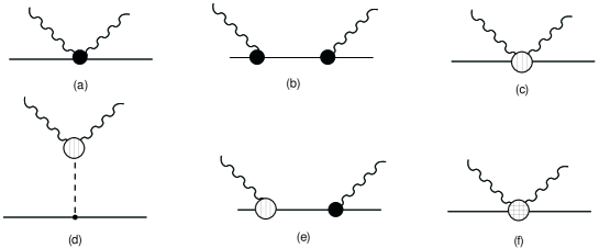
Figure 1: Tree diagrams that contribute to Compton scattering in the $\epsilon\cdot v=0$ gauge up to $O(Q^{4})$. Small dots are vertices from ${\cal L}^{(0)}$, larger dots are vertices from ${\cal L}^{(1)}$, the sliced dots are vertices from ${\cal L}^{(2)}$ and the sliced and diced dots are vertices from ${\cal L}^{(3)}$. Crossed graphs and graphs which differ only in the ordering of vertices from ${\cal L}^{(1)}$ and ${\cal L}^{(2)}$ are included in the calculation, but are not shown here.

In heavy-baryon chiral perturbation theory the amplitudes $A_{1}$–$A_{6}$ include the tree contributions shown in Fig. 1, and the pion-loop contributions of Fig. 2. At $O(Q^{2})$ only graph 1(a) contributes, and this reproduces the spin-independent low-energy theorem for Compton scattering from a single nucleon—the Thomson limit:

$$T_{\gamma N}=-{\vec{\epsilon}}\cdot{\vec{\epsilon}\,^{\prime}}\frac{{\cal Z}^{2}e^{2}}{M},$$ (22)

where ${{\cal Z}}$ is the nucleon charge in units of $|e|$.

Figure 2: Diagrams which contribute to nucleon Compton scattering in the $\epsilon\cdot v=0$ gauge at 3rd (i-iv) and 4th (a-s) order. Vertices are labeled as in Fig. 1.

At $O(Q^{3})$ the s-channel proton-pole diagram, Fig. 1(b), and its crossed u-channel partner, together with a $\gamma N$ seagull from ${\cal L}^{(2)}$ (Fig. 1(c)) ensure that HB$\chi$PT recovers the Low, Gell-Mann and Goldberger low-energy theorem for spin-dependent Compton scattering [49]. At $O(Q^{3})$ the t-channel pion-pole graph Fig. 1(d) also enters; its contribution, which varies rapidly with energy, is often included in the definition of the spin polarizabilities and is the reason that the backward spin polarizability is so much larger in magnitude than the forward one. Pion-loop graphs enter first at $O(Q^{3})$— see graphs i-iv of Fig. 2—and give energy-dependent contributions to the amplitude which include the well-known predictions for the spin-independent polarizabilities of Eq. (3), as well as less-famous predictions for $\gamma_{1}$–$\gamma_{4}$ [10]. The third-order loop amplitude of Refs. [9, 12] is obtained from diagrams 2(i)–2(iv)—together with graphs related to them by crossing and alternative time-ordering of vertices—and is given in Appendix A. As observed in Ref. [25], the $O(Q^{3})$ $\chi$PT result for $\gamma$p scattering is in good agreement with the data at forward angles up to quite high energies ($\sim 200$ MeV), but fails to describe the backward-angle data already at around 100 MeV.

At $O(Q^{4})$ in HB$\chi$PT nucleon pole graphs 1(e) and the fixed-coefficient piece of the seagull depicted in Fig. 1(f) give further terms in the $1/M$-expansion of the relativistic Born amplitude. There are also a number of fourth-order one-pion loop graphs (graphs a-r of Fig. 2), which—with one exception—contribute only to the “structure” part of the $\gamma N$ amplitude. (The exception is graph 2g which also renormalizes $\kappa$ in the spin-dependent Born amplitude.) All of the graphs 2a–2r involve vertices from ${\cal L}^{(1)}$ of Eq. (13). In particular, the expressions for diagrams 2n–2r contain the LECs $c_{1}$, $c_{2}$, and $c_{3}$, and in diagrams 2e–2g the nucleon anomalous magnetic moments enter.

Divergences in graphs 2a–2f, 2h–2k, 2p, and 2q need to be renormalized by the counterterms appearing in Eq. (15). The divergent fourth-order loop contributions to the spin-independent polarizabilities—first derived in Ref. [11]—are as follows:

$$(\alpha+\beta)^{(4)}_{\rm loop}\,\,:\,\,{e^{2}\over 4\pi f_{\pi}^{2}}\left({g_{A}^{2}\over 12M}\Bigl{(}(d^{2}+8d-1)+(12\mu_{s}+2d+4)\tau_{3}\Bigr{)}-\frac{2}{3}\tilde{c}_{2}\right)\Delta_{\pi}^{\prime};$$

$$\beta^{(4)}_{\rm loop}\,\,:\,\,{e^{2}\over 4\pi f_{\pi}^{2}}\left({g_{A}^{2}\over 24M}\Bigl{(}-d^{2}+10d+23+24\mu_{s}\tau_{3}\Bigr{)}-\frac{1}{3}\Bigl{(}\tilde{c}_{2}+(d-4)(c_{3}-2c_{1})\Bigr{)}\right)\Delta_{\pi}^{\prime},$$

where $d$ is the space-time dimension,

$$\Delta_{\pi}^{\prime}=(d-2)L(\mu)+(1/8\pi^{2})\log\left({m_{\pi}\over\mu}\right),$$ (24)

$\mu$ is the renormalization scale, and

$$(d-4)L(\mu)=(1/16\pi^{2})+O(d-4).$$ (25)

Now adding the counterterms from ${\cal L}^{(3)}$ of Eq. (15) cancels the divergences, leaving:

$$4\pi(\alpha+\beta)^{(4)} = {e^{2}\over 16\pi^{2}f_{\pi}^{2}}\left({g_{A}^{2}\over 12M}\Bigl{(}(94+24(\mu_{s}+1)\tau_{3})\log\left({m_{\pi}\over\mu}\right)+79+(16+12\mu_{s})\tau_{3}\Bigr{)}\right.$$

$$\left.-\frac{2}{3}\tilde{c}_{2}\Bigl{(}2\log\left({m_{\pi}\over\mu}\right)+1\Bigr{)}\right)+\delta\alpha_{N}(\mu)+\delta\beta_{N}(\mu)+\tau_{3}\left(\delta\alpha_{v}(\mu)+\delta\beta_{v}(\mu)\right);$$

$$4\pi\beta^{(4)} = {e^{2}\over 16\pi^{2}f_{\pi}^{2}}\left({g_{A}^{2}\over 24M}\Bigl{(}(94+48\mu_{s}\tau_{3})\log\left({m_{\pi}\over\mu}\right)+51+24\mu_{s}\tau_{3}\Bigr{)}\right.$$

$$\qquad\quad\left.-\frac{2}{3}\tilde{c}_{2}\log\left({m_{\pi}\over\mu}\right)-\frac{1}{3}(\tilde{c}_{2}+2c_{3}-4c_{1})\right)+\delta\beta_{N}(\mu)+\tau_{3}\delta\beta_{v}(\mu),$$

with $\tilde{c}_{2}=c_{2}-\frac{g_{A}^{2}}{8M}$.

The scale dependence in the LECs $\delta\alpha_{N,v}$ and $\delta\beta_{N,v}$ cancels the $\mu$-dependence of the loop pieces. The $\gamma N$ seagulls proportional to these LECs (Fig. 1(f)) represent contributions to $\alpha$ and $\beta$ from mechanisms other than soft-pion loops, i.e. short-distance effects. As such they should, strictly speaking, be determined from data, since they contain physics that is outside the purview of the EFT. In contrast the spin polarizabilities, as well as all higher terms in the Taylor-series expansion of the Compton amplitude, are still predictive in $\chi$PT at this order—as long as the values of the $c_{i}$’s are taken from some other process. The first short-distance effects in $\gamma_{1}$–$\gamma_{4}$ occur at $O(Q^{5})$.

The full amplitudes at $O(Q^{4})$ are too lengthy to be given here; they can be constructed from the information given in the appendix of Ref. [12] and the details given in Appendices B and C. We stress that in what follows it is always the full $O(Q^{4})$ HB$\chi$PT amplitude, and not a Taylor-series expansion such as (21), which is employed.

A well-known problem with the heavy-baryon approach is that at finite order the pion-production threshold comes at $\omega=m_{\pi}$. Furthermore beyond third order the amplitudes diverge at that point. The solution is to resum the terms which, taken together to all orders, would shift the threshold to the physical point $\omega_{\rm th}$; in practice this involves writing the amplitudes as functions of $\omega/\omega_{\rm th}$ instead of $\omega/m_{\pi}$, then Taylor-expanding to correct the error introduced to appropriate order. The resulting amplitudes are then finite and have the threshold in the correct place. This procedure was first introduced for forward scattering in Ref. [10], and elaborated for non-forward scattering in Ref. [12]. Since the proton data fitted spans the pion-production threshold we used this procedure for the extraction of the proton polarizabilities, but as the highest energy in the deuteron case is only 95 MeV, we did not do so in that case.

Having obtained the amplitudes, the differential cross section in any frame is a kinematic prefactor $\Phi^{2}$ times the invariant $|T|^{2}$. Experimental data, though taken in the lab frame, are sometimes presented as c.m.-frame differential cross sections, so both prefactors are needed:

$$\Phi_{\rm lab}={1\over 4\pi}{E_{\gamma}^{\prime}\over E_{\gamma}};\qquad\qquad\Phi_{\rm cm}={1\over 4\pi}{M\over\sqrt{s}}.$$ (27)

Finally, in terms of the Breit-frame $A_{1}$–$A_{6}$, $|T|^{2}$ is given by:

$$|T|^{2} = {\textstyle{1\over 2}}A_{1}^{2}(1+\cos^{2}\theta)+{\textstyle{1\over 2}}A_{3}^{2}(3-\cos^{2}\theta)$$ (28)

$$+\sin^{2}\theta\,\bigl{[}4A_{3}A_{6}+(A_{3}A_{4}+2A_{3}A_{5}-A_{1}A_{2})\cos\theta\bigr{]}$$

$$+\sin^{2}\theta\,\bigl{[}{\textstyle{1\over 2}}A_{2}^{2}\sin^{2}\theta+{\textstyle{1\over 2}}A_{4}^{2}(1+\cos^{2}\theta)+A_{5}^{2}(1+2\cos^{2}\theta)+3A_{6}^{2}$$

$$\kern 56.9055pt+2A_{6}(A_{4}+3A_{5})\cos\theta+2A_{4}A_{5}\cos^{2}\theta\bigr{]}.$$

(Above the $\pi N$ threshold one should replace $A_{i}^{2}$ by $|A_{i}|^{2}$ and $A_{i}A_{j}$ by $\Re(A_{i}^{*}A_{j})$.)

4 Compton scattering on the proton: results

The only unknowns in the $O(Q^{4})$ $\chi$PT $\gamma$p amplitude are $\delta\alpha_{p}$ and $\delta\beta_{p}$, since the values of $c_{1}$, $c_{2}$, and $c_{3}$ can be determined from $\pi N$ [39] (or $NN$ [40]) scattering data. If these counterterms are combined with the (scale-dependent) divergences they renormalize we can regard $\alpha_{p}$ and $\beta_{p}$ (or, more precisely, the shifts of the polarizabilities from their $O(Q^{3})$ values) as the two free parameters in the $O(Q^{4})$ calculation.

In Ref. [12], these two free parameters were not fit directly. Rather, the input to that calculation included the Particle Data Group (PDG) values of the polarizabilities [50]. The resulting differential cross sections are in good agreement with the low-energy data.

While these PDG values are derived from polarizabilities quoted in experimental papers, the energies of the relevant experiments are, for the most part, too high for a direct fit to the polynomial form (21). Instead the amplitudes these papers employ in order to extract $\alpha_{p}$ and $\beta_{p}$ are based on dispersion relations, using plausible assumptions about their asymptotic form coupled with models for those amplitudes which do not converge. The difference $\alpha_{p}-\beta_{p}$ is a parameter in these fits; the sum is (usually) taken from the Baldin sum rule [51].

This approach implicitly builds in model-dependent assumptions about the behavior of the $\gamma$p amplitude beyond the low-energy regime. In what follows we adopt a different strategy, using $\chi$PT to determine the polarizabilities from only low-energy ($\omega\leq 200$ MeV) differential cross sections, so as to obtain truly model-independent results for $\alpha_{p}$ and $\beta_{p}$.

In a recent paper the world data on proton Compton scattering was examined, and it was demonstrated that data from the 1950s and 1960s is compatible with the more modern data from 1974 on, and is useful in reducing errors [52]. We have therefore used all the data in Table 2 of Ref. [52], with the exception of the first three points for which the normalization error is not known. We have also included higher-energy points from the experiments of Refs. [17], and the TAPS data [18].

All the experiments have an overall normalization error. We incorporate this by adding a piece to the usual $\chi^{2}$ function:

$$\chi^{2} = \chi^{2}_{\rm stat.}+\chi^{2}_{\rm syst.}$$ (29)

$$= \sum_{j=1}^{N_{\rm sets}}\sum_{i=1}^{N_{j}}\left(\frac{{\cal N}_{j}({\rm d}\sigma_{ij}/{\rm d}\Omega)_{\rm expt}-({\rm d}\sigma_{ij}/{\rm d}\Omega)_{\rm theory}}{{\cal N}_{j}\Delta_{ij}}\right)^{2}+\sum_{j=1}^{N_{\rm sets}}\left(\frac{{\cal N}_{j}-1}{{\cal N}_{j}\delta_{j}}\right)^{2},$$

where ${\rm d}\sigma_{ij}$ and $\Delta_{ij}$ are the value and statistical error of the $i$th observation from the $j$th experimental set, $\delta_{j}$ is the fractional systematic error of set $j$, and ${\cal N}_{j}$ is an overall normalization for set $j$. The additional parameters ${\cal N}_{j}$ are to be optimized by minimizing the combined $\chi^{2}$. This can be done analytically, leaving a $\chi^{2}$ that is a function of $\alpha_{p}$ and $\beta_{p}$ alone. Since we fit 13 $\gamma$p data sets this reduces the number of degrees of freedom in the final minimization by 13. (For more details on this formalism see Ref. [52].)

In Ref. [12] it was found that while the $\chi$PT fit was very good at sufficiently low energies and forward angles, it failed for higher energies and backward angles, and did so in a way that could not be remedied by adjusting parameters. This suggests that at a relatively low momentum “new” physics is coming in—an observation that is consistent with the Delta-nucleon mass difference being only a factor of two larger than $m_{\pi}$. Indeed, in both existing models and the effective field theory with explicit Delta-isobar degrees of freedom [35, 64] Delta effects appear at backward angles already at $\omega\sim m_{\pi}$. (Their impact on the forward-angle data does not show up until higher energies are reached.) As a consequence in our extraction of $\alpha_{p}$ and $\beta_{p}$ we impose a cut on both the photon energy and the momentum transfer, $\omega,\,\sqrt{|t|}\leq\omega_{\rm max}$.

We investigated the effect of varying $\omega_{\rm max}$ between 140 and 200 MeV—see Table 1. As $\omega_{\rm max}$ was increased the central values of $\alpha_{p}$ and $\beta_{p}$ changed very little; the 1-$\sigma$ curve tightened as more data were included, but the $\chi^{2}/{\rm d.o.f}$ of the best-fit point tended to rise. This did not seem to be due to a systematic worsening of the fit, but rather to the inclusion of rather noisy data. We have chosen to quote the central value corresponding to a cut-off of $\omega_{\rm max}=180$ MeV, for which $\chi^{2}/{\rm d.o.f}$ was (locally) minimized at $133/113$. This fit is shown in Fig. 3 together with the low-energy data.

$\omega_{\rm max}$ (MeV)	$N_{\rm data}$	$\alpha_{p}$ ($10^{-4}$ fm3)	$\beta_{p}$ ($10^{-4}$ fm3)	$\chi^{2}$/d.o.f.
200	144	11.7	3.40	1.32
180	126	12.1	3.38	1.18
165	109	12.3	3.37	1.27
140	73	12.0	3.13	1.26

Table 1: Results of $O(Q^{4})$ fits for $\alpha_{p}$ and $\beta_{p}$ to world $\gamma$p data over various ranges $\omega,\sqrt{|t|}<\omega_{\rm max}$. In each case $N_{\rm data}$ is the number of data points included in the fit.

Figure 3: Results of the $O(Q^{4})$ EFT best fit to the differential cross sections for Compton scattering on the proton at various angles, compared to the experimental data [17, 18]. The gray region is excluded from the fit. The magenta diamonds are Mainz data [18]; the other symbols are explained in Ref. [12].

The best-fit point for the proton electric and magnetic polarizabilities is shown in Fig. 4, together with the 1-$\sigma$ curve ($\chi^{2}_{\rm min}+2.28$):

$$\alpha_{p} = (12.1\pm 1.1)_{-0.5}^{+0.5}\times 10^{-4}\,{\rm fm}^{3},$$

$$\beta_{p} = (3.4\pm 1.1)_{-0.1}^{+0.1}\times 10^{-4}\,{\rm fm}^{3}.$$ (30)

Statistical (1-$\sigma$) errors are inside the brackets. An estimate of the theoretical error due to truncation of the expansion at $O(Q^{4})$ is given outside the brackets. The result (30) is fully compatible with other extractions, although the central value of $\beta_{p}$ is somewhat phigher [50, 53].

This theoretical error is assessed by varying the bound on which data are fit from 140 MeV to 200 MeV. The size inferred thereby is consistent with estimates of the impact that $O(Q^{5})$ terms would have on the fit. In this context it is worth noting that although the $O(Q^{4})$ $\chi$PT predictions for the spin polarizabilities $\gamma_{1}$–$\gamma_{4}$ are not in good agreement with those obtained from other sources, in Ref. [12] it was shown that at the energies considered here the differential cross section is largely insensitive to their values. (Asymmetries in polarised Compton scattering would be far more sensitive.)

The recent re-evaluation of the Baldin sum rule [51] by Olmos de León et al. [18] gives:

$$\alpha_{p}+\beta_{p}=(13.8\pm 0.4)\times 10^{-4}~{}{\rm fm}^{3}.$$ (31)

If one considers only statistical errors the results (30) and (31) are marginally inconsistent at the 1-$\sigma$ level—see Fig. 4. Our values for $\alpha_{p}$ and $\beta_{p}$ are consistent with the constraint (31) once the potential impact of theoretical uncertainties is taken into account.

Figure 4: Values (in $10^{-4}\,{\rm fm}^{3}$) of the proton magnetic and electric polarizabilities extracted from an $O(Q^{4})$ EFT fit to low-energy cross-section data, together with the values allowed by the Baldin sum-rule constraint (31) (gray shaded area).

Including the constraint (31) in our fit leads to values for $\alpha_{p}$ and $\beta_{p}$ consistent with Eq. (30), but with smaller statistical errors, namely:

$$\alpha_{p} = (11.0\pm 0.5\pm 0.2)_{-0.5}^{+0.5}\times 10^{-4}\,{\rm fm}^{3},$$

$$\beta_{p} = (2.8\pm 0.5\mp 0.2)_{-0.1}^{+0.1}\times 10^{-4}\,{\rm fm}^{3}.$$ (32)

In Eq. (32) we have left the systematic error unchanged, but have now included a second error inside the brackets, whose source is the error on the sum-rule evaluation (31). The smaller statistical errors are achieved at the expense of introducing certain assumptions about the high-energy behavior of the Compton amplitude into the result, via the use of the Baldin sum-rule result (31). The result (32) is in excellent agreement with a recent determination of $\alpha_{p}$ and $\beta_{p}$ which used an effective field theory with explicit Delta degrees of freedom to fit all $\gamma$p scattering data up to $\omega\sim 170$ MeV [36].

5 Compton scattering on the deuteron: theory

In this section we concentrate on real Compton scattering on an $A=2$ system.

The leading contributions to the irreducible $\gamma NN\rightarrow\gamma NN$ kernel $K_{\gamma\gamma}$ appear at $\nu=-1$—$O(Q^{2})$—from a tree-level diagram ($L=0$) with two separately connected pieces ($C=2$) and a vertex which is the two-photon seagull of $\Delta_{i}=1$. This vertex arises from minimal coupling in the kinetic nucleon terms in ${\cal L}^{(1)}$ of Eq. (13)—see Fig. 5(a). It therefore represents Compton scattering on the $NN$ system where the neutron is a spectator while the photon scatters from the proton via the Thomson amplitude (22).

Figure 5: Characteristic one-body interactions that contribute to Compton scattering on the deuteron at order $Q^{2}$ (a) and at order $Q^{3}$ (b-e) (in the Coulomb gauge). Crossed graphs are not shown and not all loop topologies are shown. The sliced blobs are vertex insertions from ${\cal L}^{(1)}$. The sliced and diced blobs are vertex insertions from ${\cal L}^{(2)}$.

Figure 6: Two-body interactions which contribute to Compton scattering on the deuteron at order $Q^{3}$ ($\nu=0$) in Coulomb gauge. Graphs which differ only by interchange of the nucleons are not shown.

At orders $\nu\geq 0$ there are two classes of corrections: corrections to the one-nucleon amplitude where the second nucleon is just a spectator, and corrections that involve both nucleons. Shown in Fig. 5(b-e) are the one-nucleon corrections at $\nu=0$, while Fig. 6 displays two-nucleon corrections of the same order. Note that the one-nucleon-loop and two-nucleon diagrams involve only $\Delta_{i}=0$ interactions in diagrams with $L=1$ or $C=1$.

At this, or indeed any, order the irreducible $\gamma NN\rightarrow\gamma NN$ kernel can be separated into one- and two-body pieces. Doing this in the $\gamma NN$ c.m. frame, with the kinematics shown in Fig. 7 we obtain:

$$K_{\gamma\gamma}^{\gamma NNc.m.}({{\vec{p}}\,^{\prime}},{{\vec{k}}^{\,\prime}};{\vec{p}},{\vec{k}})=T^{\gamma d\,c.m.}_{\gamma N}({{\vec{k}}^{\,\prime}};{\vec{k}})\,\,\delta^{(3)}\left(p^{\prime}-p-{\textstyle{1\over 2}}q\right)+T^{2N}_{\gamma NN}({{\vec{p}}\,^{\prime}},{{\vec{k}}^{\,\prime}};{\vec{p}},{\vec{k}});$$ (33)

with $\vec{q}\equiv\vec{k}-{{\vec{k}}^{\,\prime}}$ the momentum transfer of the Compton scattering process. The one-nucleon piece $T^{\gamma d\,c.m.}_{\gamma N}({{\vec{k}}^{\,\prime}};{\vec{k}})$ is related to the $\gamma N$ amplitude discussed in Sec. 3 by a boost from the Breit frame to the $\gamma$d c.m. frame. Details of the boosting procedure are given in the Appendices.

Figure 7: Kinematics for the $\gamma$d process in the $\gamma$d center-of-mass frame. The sliced circle represents $K_{\gamma\gamma}$, the irreducible $\gamma NN\rightarrow\gamma NN$ kernel.

Meanwhile $T_{\gamma NN}^{2N}$ was computed to third order in small quantities in Ref. [15]. At fourth order the difference of initial and final nucleon kinetic energies should be included in the pion propagators appearing in Fig. 6. The result is then:

$$T_{\gamma NN,\,O(Q^{3})}^{2N}\;=\;-\frac{{e^{2}}{g_{\scriptscriptstyle A}^{2}}}{2f_{\pi}^{2}}\;({\vec{\tau}}^{\;1}\cdot{\vec{\tau}}^{\;2}-\tau^{1}_{z}\tau^{2}_{z})\;(t^{(a)}+t^{(b)}+t^{(c)}+t^{(d)}+t^{(e)})$$ (34)

with:

$${t^{(a)}} = \frac{{{\vec{\epsilon}}\cdot{\vec{\sigma}^{\scriptscriptstyle 1}}}\;{{\vec{\epsilon}\,^{\prime}}\cdot{\vec{\sigma}^{\scriptscriptstyle 2}}}}{2[\tilde{\omega}^{2}-{m_{\pi}^{2}}-({\vec{p}}-{{\vec{p}}\,^{\prime}}+{\vec{k}}_{+})^{2}]}+(1\;\leftrightarrow\;2)$$

$${t^{(b)}} = \frac{{{\vec{\epsilon}}\cdot{\vec{\epsilon}\,^{\prime}}}\;{\vec{\sigma}^{\scriptscriptstyle 1}}\cdot({\vec{p}}-{{\vec{p}}\,^{\prime}}-{\textstyle{1\over 2}}\vec{q}^{\,}){\vec{\sigma}^{\scriptscriptstyle 2}}\cdot({\vec{p}}-{{\vec{p}}\,^{\prime}}+{\textstyle{1\over 2}}\vec{q}^{\,})}{2[({\vec{p}}-{{\vec{p}}\,^{\prime}}-{\textstyle{1\over 2}}\vec{q}^{\,})^{2}+{m_{\pi}^{2}}][({\vec{p}}-{{\vec{p}}\,^{\prime}}+{\textstyle{1\over 2}}\vec{q}^{\,})^{2}+m_{\pi}^{2}]}+(1\;\leftrightarrow\;2)$$

$${t^{(c)}} = -\frac{{{\vec{\epsilon}\,^{\prime}}\cdot({\vec{p}}-{{\vec{p}}\,^{\prime}}+{\frac{1}{2}{\vec{k}}})}\;{\vec{\sigma}^{\scriptscriptstyle 1}}\cdot{\vec{\epsilon}}\;{\vec{\sigma}^{\scriptscriptstyle 2}}\cdot({\vec{p}}-{{\vec{p}}\,^{\prime}}+{\textstyle{1\over 2}}\vec{q}^{\,})}{[\tilde{\omega}^{2}-m_{\pi}^{2}-({\vec{p}}-{{\vec{p}}\,^{\prime}}+\vec{k}_{+})^{2}][({\vec{p}}-{{\vec{p}}\,^{\prime}}+\frac{1}{2}\vec{q}^{\,})^{2}+m_{\pi}^{2}]}+(1\;\leftrightarrow\;2)$$

$${t^{(d)}} = -\frac{{{\vec{\epsilon}}\cdot({\vec{p}}-{{\vec{p}}\,^{\prime}}+{{\textstyle{1\over 2}}{{\vec{k}}^{\,\prime}}})}\;{\vec{\sigma}^{\scriptscriptstyle 1}}\cdot({\vec{p}}-{{\vec{p}}\,^{\prime}}-{{\textstyle{1\over 2}}\vec{q}^{\,})}){\vec{\sigma}^{\scriptscriptstyle 2}}\cdot{\vec{\epsilon}\,^{\prime}}}{[\tilde{\omega}^{2}-{m}_{\pi}^{2}-({\vec{p}}-{{\vec{p}}\,^{\prime}}+\vec{k}_{+})^{2}][({\vec{p}}-{{\vec{p}}\,^{\prime}}-{\textstyle{1\over 2}}\vec{q}^{\,})^{2}+m_{\pi}^{2}]}+(1\;\leftrightarrow\;2)$$

$${t^{(e)}} = \frac{{\vec{\sigma}^{\scriptscriptstyle 1}}\cdot({\vec{p}}-{{\vec{p}}\,^{\prime}}-{\textstyle{1\over 2}}\vec{q}^{\,})\;{\vec{\sigma}^{\scriptscriptstyle 2}}\cdot({\vec{p}}-{{\vec{p}}\,^{\prime}}+{\textstyle{1\over 2}}\vec{q}^{\,})}{[({\vec{p}}-{{\vec{p}}\,^{\prime}}-{\textstyle{1\over 2}}\vec{q}^{\,})^{2}+{m_{\pi}^{2}}][({\vec{p}}-{{\vec{p}}\,^{\prime}}+{\textstyle{1\over 2}}\vec{q}^{\,})^{2}+{m_{\pi}^{2}}]}$$ (35)

$$\qquad\qquad\qquad\times\frac{2\;{\vec{\epsilon}}\cdot({\vec{p}}-{{\vec{p}}\,^{\prime}}+{\frac{1}{2}{{\vec{k}}^{\,\prime}}})\;{\vec{\epsilon}\,^{\prime}}\cdot({\vec{p}}-{{\vec{p}}\,^{\prime}}+{\frac{1}{2}{\vec{k}}})}{[\tilde{\omega}^{2}-{m_{\pi}^{2}}-({\vec{p}}-{{\vec{p}}\,^{\prime}}+\vec{k}_{+})^{2}]}\;+\;(1\;\leftrightarrow\;2),$$

where $\vec{k}_{+}\equiv{\textstyle{1\over 2}}({\vec{k}}+{{\vec{k}}^{\,\prime}})$ is the average of incoming and outgoing photon three-momenta, the notation $(1\leftrightarrow 2)$ indicates the inclusion of a second term in which ${\vec{p}}\rightarrow-{\vec{p}}$, ${{\vec{p}}\,^{\prime}}\rightarrow-{{\vec{p}}\,^{\prime}}$, ${\vec{\sigma}^{\scriptscriptstyle 1}}\leftrightarrow{\vec{\sigma}^{\scriptscriptstyle 2}}$, and:

$$\tilde{\omega}^{2}\equiv\omega^{2}+\omega\,\frac{{{\vec{p}}\,^{\prime}}\cdot{{\vec{k}}^{\,\prime}}-{\vec{p}}\cdot{\vec{k}}}{M}.$$ (36)

In computing the “retardation” effects which modify modify $\omega\to\tilde{\omega}$ we use the fact that—because we are considering an elastic process—the two-nucleon initial and final states are equally distant from being on-shell. Thus the results (35), (36) were derived using $|{\vec{p}}^{\,}|^{2}=|{{\vec{p}}\,^{\prime}}|^{2}$, which simplifies the expression for $\tilde{\omega}$. Note that for virtual momenta ${\vec{p}}$ and ${{\vec{p}}\,^{\prime}}$ of order $M$ the retardation effects included here will have unphysical consequences, and thus Eq. (36) is only valid if $|{\vec{p}}^{\,}|,|{{\vec{p}}\,^{\prime}}|\ll M$.

Upon including these retardation effects in our calculation we found them to be numerically very small. Hence in the computations of the $\gamma$d differential cross section which we report on below they were not considered.

Since neither the expression for $T^{2N}_{\gamma NN,O(Q^{3})}$ nor the $\gamma N$ $O(Q^{3})$ amplitude contain any free parameters, $\chi$PT makes predictions for $\gamma$d scattering at this order. These predictions were generated in Ref. [15] and compared to the data of Ref. [19], with encouraging results, especially at $E_{\rm lab}=69$ MeV. The $O(Q^{3})$ predictions (made on the basis of Ref. [15]) for the Lund experiments at $\omega\approx 55$ MeV and $\omega\approx 66$ MeV turned out to be in excellent agreement with that data too. (See curves below.)

At $O(Q^{4})$ there are many one-nucleon diagrams in the $\gamma NN$ kernel, which are easily obtained from those in Figs. 1 and 2. These were computed in the Breit frame in Ref. [12]. The extra pieces of the $\gamma N$ amplitude which are obtained in the $\gamma$d center-of-mass frame as compared to the Breit-frame result are discussed in Appendices A–D.

Two-nucleon diagrams at $O(Q^{4})$ in Coulomb gauge are depicted in Figs. 8 and 9. These two-nucleon $\nu=1$ diagrams have $C=1$ with one insertion from ${\cal L}^{(1)}$.

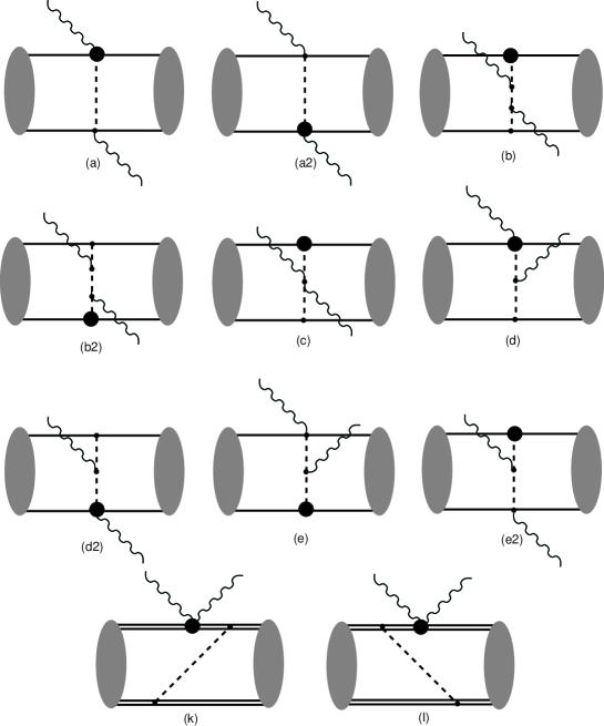
Figure 8: Some of the two-body graphs that are nominally $O(Q^{4})$ for $\gamma$d scattering in Coulomb gauge. Ultimately all of the graphs shown here are either identically zero or suppressed to $O(Q^{5})$ by kinematic effects, as explained in the text. Non-zero two-body contributions to $\gamma$d scattering at $O(Q^{4})$ are shown in Fig. 9. .

Although they are nominally of $O(Q^{4})$, all of the graphs in Fig. 8 give zero contribution to the elastic $\gamma$d amplitude at this order. Diagrams (a), (a2), (d), and (d2) do not affect this process because $K_{\gamma\gamma}$ is of isovector character. Meanwhile graphs (b), (b2), (c), (e), and (e2) all involve the $\pi NN$ vertex from ${\cal L}^{(1)}$. With the choice $v=(1,\vec{0})$ the Feynman rule for this vertex reads:

$$\frac{g_{A}}{4Mf_{\pi}}\,\vec{\sigma}\cdot(\vec{p}+{{\vec{p}}\,^{\prime}})\,q_{0}\,\tau^{a},$$ (37)

where $\vec{p}$ (${{\vec{p}}\,^{\prime}}$) is the nucleon momentum before (after) the emission of the pion, and $q$ is the emitted pion’s four-momentum. In the context of the $\gamma NN$ kernel being discussed here the emitted pion is a “potential” pion [31], and as such has $q_{0}\sim{{\vec{p}}\,}^{2}/M$. Consequently in the kinematics we are considering all five of these graphs are suppressed to $O(Q^{5})$. Lastly, graphs (k) and (l) represent time-orderings where the photon interacts with a single nucleon while the pion is “in-flight”. If, as is the case here, an instantaneous potential is employed to generate the deuteron wave function then consistency between the potential $V$ and the $\gamma NN\rightarrow\gamma NN$ kernel requires that graphs (k) and (l) not be included in $K_{\gamma\gamma}$.

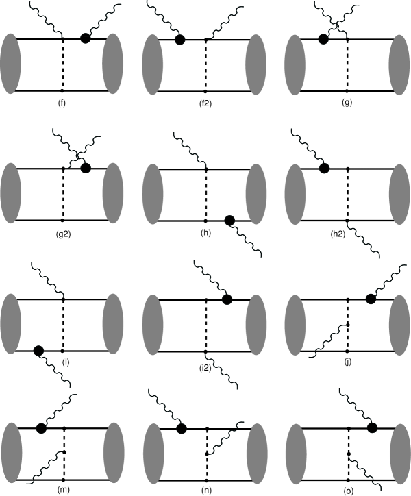
Figure 9: The two-body diagrams contributing to $\gamma$d scattering in Coulomb gauge at $O(Q^{4})$.

The non-zero two-body graphs at $O(Q^{4})$ are depicted in Fig. 9. The ($\gamma$d c.m. frame) expressions for these pieces of the irreducible $\gamma NN\rightarrow\gamma NN$ kernel sum to:

$$T_{\gamma NN,\,O(Q^{4})}^{2N}\;=\;\;\frac{{e^{2}}{g_{\scriptscriptstyle A}^{2}}}{4f_{\pi}^{2}}\;\frac{1}{M\omega}\;({\vec{\tau}}^{\;1}\cdot{\vec{\tau}}^{\;2}-\tau^{1}_{z}\tau^{2}_{z})\;(t^{(f+g)}+t^{(f_{2}+g_{2})}+t^{(h+i+h_{2}+i_{2})}+t^{(j+m)}+t^{(n+o)}),$$ (38)

with:

$$t^{(f+g)} = -\frac{1}{2[(\vec{p}-{{\vec{p}}\,^{\prime}}+{\textstyle{1\over 2}}\vec{q}^{\,})^{2}+m_{\pi}^{2}]}\{{\vec{\epsilon}\,^{\prime}}\cdot({\vec{p}}+{{\vec{p}}\,^{\prime}}-\vec{k}_{+})$$

$$\times[{\vec{\sigma}^{\scriptscriptstyle 1}}\cdot(\vec{p}-{{\vec{p}}\,^{\prime}}+{\textstyle{1\over 2}}\vec{q}^{\,}){\vec{\sigma}^{\scriptscriptstyle 2}}\cdot{\vec{\epsilon}}+{\vec{\sigma}^{\scriptscriptstyle 2}}\cdot(\vec{p}-{{\vec{p}}\,^{\prime}}+{\textstyle{1\over 2}}\vec{q}^{\,}){\vec{\sigma}^{\scriptscriptstyle 1}}\cdot{\vec{\epsilon}}]$$

$$+i(1+\kappa_{v}){\vec{\epsilon}}\cdot({\vec{\epsilon}\,^{\prime}}\times{{\vec{k}}^{\,\prime}})({\vec{\sigma}^{\scriptscriptstyle 1}}+{\vec{\sigma}^{\scriptscriptstyle 2}})\cdot(\vec{p}-{{\vec{p}}\,^{\prime}}+{\textstyle{1\over 2}}\vec{q}^{\,})\}$$

$$t^{(f_{2}+g_{2})} = \frac{1}{2[(\vec{p}-{{\vec{p}}\,^{\prime}}+{\textstyle{1\over 2}}\vec{q}^{\,})^{2}+m_{\pi}^{2}]}\{{\vec{\epsilon}}\cdot({\vec{p}}+{{\vec{p}}\,^{\prime}}-\vec{k}_{+})$$

$$\times[{\vec{\sigma}^{\scriptscriptstyle 1}}\cdot(\vec{p}-{{\vec{p}}\,^{\prime}}+{\textstyle{1\over 2}}\vec{q}^{\,}){\vec{\sigma}^{\scriptscriptstyle 2}}\cdot{\vec{\epsilon}\,^{\prime}}+{\vec{\sigma}^{\scriptscriptstyle 2}}\cdot(\vec{p}-{{\vec{p}}\,^{\prime}}+{\textstyle{1\over 2}}\vec{q}^{\,}){\vec{\sigma}^{\scriptscriptstyle 1}}\cdot{\vec{\epsilon}\,^{\prime}}]$$

$$-i(1+\kappa_{v}){\vec{\epsilon}\,^{\prime}}\cdot({\vec{\epsilon}}\times{\vec{k}})({\vec{\sigma}^{\scriptscriptstyle 1}}+{\vec{\sigma}^{\scriptscriptstyle 2}})\cdot(\vec{p}-{{\vec{p}}\,^{\prime}}+{\textstyle{1\over 2}}\vec{q}^{\,})\}$$

$$t^{(h+i+h_{2}+i_{2})} = \frac{1}{2[\omega^{2}-m_{\pi}^{2}-(\vec{p}-{{\vec{p}}\,^{\prime}}+\vec{k}_{+})^{2}]}\{{\vec{\epsilon}\,^{\prime}}\cdot({\vec{p}}+{{\vec{p}}\,^{\prime}}+\vec{k}_{+})$$

$$\times[{\vec{\sigma}^{\scriptscriptstyle 1}}\cdot(\vec{p}-{{\vec{p}}\,^{\prime}}+\vec{k}_{+}){\vec{\sigma}^{\scriptscriptstyle 2}}\cdot{\vec{\epsilon}}+{\vec{\sigma}^{\scriptscriptstyle 2}}\cdot(\vec{p}-{{\vec{p}}\,^{\prime}}+\vec{k}_{+}){\vec{\sigma}^{\scriptscriptstyle 1}}\cdot{\vec{\epsilon}}]$$

$$-i(1+\kappa_{v})(\vec{p}-{{\vec{p}}\,^{\prime}}+\vec{k}_{+})\cdot({\vec{\epsilon}\,^{\prime}}\times{{\vec{k}}^{\,\prime}})\,({\vec{\sigma}^{\scriptscriptstyle 1}}+{\vec{\sigma}^{\scriptscriptstyle 2}})\cdot{\vec{\epsilon}}$$

$$-{\vec{\epsilon}}\cdot({\vec{p}}+{{\vec{p}}\,^{\prime}}-\vec{k}_{+})[{\vec{\sigma}^{\scriptscriptstyle 1}}\cdot(\vec{p}-{{\vec{p}}\,^{\prime}}+\vec{k}_{+}){\vec{\sigma}^{\scriptscriptstyle 2}}\cdot{\vec{\epsilon}\,^{\prime}}$$

$$\qquad\qquad+{\vec{\sigma}^{\scriptscriptstyle 2}}\cdot(\vec{p}-{{\vec{p}}\,^{\prime}}+\vec{k}_{+}){\vec{\sigma}^{\scriptscriptstyle 1}}\cdot{\vec{\epsilon}\,^{\prime}}]$$

$$+i(1+\kappa_{v})(\vec{p}-{{\vec{p}}\,^{\prime}}+\vec{k}_{+})\cdot({\vec{\epsilon}}\times{\vec{k}})({\vec{\sigma}^{\scriptscriptstyle 1}}+{\vec{\sigma}^{\scriptscriptstyle 2}})\cdot{\vec{\epsilon}\,^{\prime}}\}$$

$$t^{(j+m)} = -\frac{1}{[\omega^{2}-m_{\pi}^{2}-(\vec{p}-{{\vec{p}}\,^{\prime}}+\vec{k}_{+})^{2}]}\frac{1}{[m_{\pi}^{2}+(\vec{p}-{{\vec{p}}\,^{\prime}}-{\textstyle{1\over 2}}\vec{q}^{\,})^{2}]}$$

$$\times{\vec{\epsilon}}\cdot({\vec{p}}-{{\vec{p}}\,^{\prime}}+\vec{k}_{+})\{{\vec{\epsilon}\,^{\prime}}\cdot({\vec{p}}+{{\vec{p}}\,^{\prime}}+\vec{k}_{+})$$

$$\times[{\vec{\sigma}^{\scriptscriptstyle 1}}\cdot(\vec{p}-{{\vec{p}}\,^{\prime}}+\vec{k}_{+}){\vec{\sigma}^{\scriptscriptstyle 2}}\cdot(\vec{p}-{{\vec{p}}\,^{\prime}}-{\textstyle{1\over 2}}\vec{q}^{\,})$$

$$\qquad\qquad+{\vec{\sigma}^{\scriptscriptstyle 2}}\cdot(\vec{p}-{{\vec{p}}\,^{\prime}}+\vec{k}_{+}){\vec{\sigma}^{\scriptscriptstyle 1}}\cdot(\vec{p}-{{\vec{p}}\,^{\prime}}-{\textstyle{1\over 2}}\vec{q}^{\,})]$$

$$-i(1+\kappa_{v})({\vec{\epsilon}\,^{\prime}}\times{{\vec{k}}^{\,\prime}})\cdot(\vec{p}-{{\vec{p}}\,^{\prime}}+\vec{k}_{+})({\vec{\sigma}^{\scriptscriptstyle 1}}+{\vec{\sigma}^{\scriptscriptstyle 2}})\cdot(\vec{p}-{{\vec{p}}\,^{\prime}}-{\textstyle{1\over 2}}\vec{q}^{\,})\}$$

$$t^{(n+o)} = \frac{1}{[\omega^{2}-m_{\pi}^{2}-(\vec{p}-{{\vec{p}}\,^{\prime}}+\vec{k}_{+})^{2}]}\frac{1}{[m_{\pi}^{2}+(\vec{p}-{{\vec{p}}\,^{\prime}}+{\textstyle{1\over 2}}\vec{q}^{\,})^{2}]}$$ (39)

$$\times{\vec{\epsilon}\,^{\prime}}\cdot({\vec{p}}-{{\vec{p}}\,^{\prime}}+\vec{k}_{+})\{{\vec{\epsilon}}\cdot({\vec{p}}+{{\vec{p}}\,^{\prime}}-\vec{k}_{+})$$

$$\times[{\vec{\sigma}^{\scriptscriptstyle 1}}\cdot(\vec{p}-{{\vec{p}}\,^{\prime}}+\vec{k}_{+}){\vec{\sigma}^{\scriptscriptstyle 2}}\cdot(\vec{p}-{{\vec{p}}\,^{\prime}}+{\textstyle{1\over 2}}\vec{q}^{\,})$$

$$\qquad\qquad+{\vec{\sigma}^{\scriptscriptstyle 2}}\cdot(\vec{p}-{{\vec{p}}\,^{\prime}}+\vec{k}_{+}){\vec{\sigma}^{\scriptscriptstyle 1}}\cdot(\vec{p}-{{\vec{p}}\,^{\prime}}+{\textstyle{1\over 2}}\vec{q}^{\,})]$$

$$-i(1+\kappa_{v})(\vec{p}-{{\vec{p}}\,^{\prime}}+\vec{k}_{+})({\vec{\epsilon}}\times{\vec{k}})({\vec{\sigma}^{\scriptscriptstyle 1}}+{\vec{\sigma}^{\scriptscriptstyle 2}})\cdot(\vec{p}-{{\vec{p}}\,^{\prime}}+{\textstyle{1\over 2}}\vec{q}^{\,})\}.$$

(In this case the contribution from diagrams related to those in Fig. 9 by interchange of the two nucleons has been explicitly included in the expressions.)

The vertices from the next-to-leading-order $\pi N$ Lagrangian which appear in these non-zero two-body diagrams all involve E1 and M1 couplings of the photon to the nucleons. Thus the only parameters appearing are the proton charge and the proton and neutron anomalous magnetic moments. There are no free parameters in the two-body $O(Q^{4})$ contribution. This is good, as these mechanisms are of the same order as the counterterms $\delta\alpha_{N}$ and $\delta\beta_{N}$ which we are trying to fit. Extracting the polarizabilities from deuteron Compton data is much more straightforward if the $O(Q^{4})$ two-body currents can be expressed in terms of known parameters.

To calculate the amplitude for $\gamma$d scattering, $T_{\gamma d}$, we first sandwich $K_{\gamma\gamma}$ between deuteron wave functions and use the decomposition of Eq. (33). This yields (in the $\gamma$d center-of-mass frame):

$$T^{\gamma d}_{M^{\prime}\lambda^{\prime}M\lambda}({{\vec{k}}^{\,\prime}},{\vec{k}}) = \int\frac{d^{3}p}{(2\pi)^{3}}\,\,\psi_{M^{\prime}}^{*}\left({\vec{p}}+{\textstyle{1\over 2}}\vec{q}^{\,}\right)\,\,T^{\gamma d\,\,c.m.}_{\gamma N_{\lambda^{\prime}\lambda}}({{\vec{k}}^{\,\prime}},{\vec{k}})\,\,\psi_{M}({\vec{p}})$$ (40)

$$+ \int\frac{d^{3}p\,\,d^{3}p^{\prime}}{(2\pi)^{6}}\,\,\psi_{M^{\prime}}^{*}({{\vec{p}}\,^{\prime}})\,\,T^{2N}_{\gamma NN_{\lambda^{\prime}\lambda}}({{\vec{k}}^{\,\prime}},{\vec{k}})\,\,\psi_{M}({\vec{p}})$$

where $M$ ($M^{\prime}$) is the initial (final) deuteron spin state, and $\lambda$ ($\lambda^{\prime}$) is the initial (final) photon polarization state, and ${\vec{k}}$ (${{\vec{k}}^{\,\prime}}$) the initial (final) photon three-momentum, which are constrained to $|{\vec{k}}|=|{{\vec{k}}^{\,\prime}}|=\omega$.

The laboratory differential cross section can then be evaluated directly:

$$\frac{d\sigma}{d\Omega_{L}}=\frac{1}{16\pi^{2}}\left(\frac{E_{\gamma}^{\prime}}{E_{\gamma}}\right)^{2}\frac{1}{6}\sum_{M^{\prime}\lambda^{\prime}M\lambda}|T^{\gamma d}_{M^{\prime}\lambda^{\prime}M\lambda}|^{2},$$ (41)

where $E_{\gamma}$ is the initial photon energy in the laboratory frame, and is related to $\omega$, the photon energy in the $\gamma$d center-of-mass frame, via:

$$\omega=\frac{E_{\gamma}}{\sqrt{1+2E_{\gamma}/M_{d}}};$$ (42)

and $E_{\gamma}^{\prime}$ is the final photon energy in the laboratory frame:

$$E_{\gamma}^{\prime}=\frac{E_{\gamma}M_{d}}{M_{d}+E_{\gamma}(1-\cos\theta_{L})}.$$ (43)

To evaluate the center-of-mass-frame differential cross section we employ:

$$\frac{d\sigma}{d\Omega_{cm}}=\frac{M_{d}}{16\pi^{2}(M_{d}+2E_{\gamma})}\frac{1}{6}\sum_{M^{\prime}\lambda^{\prime}M\lambda}|T^{\gamma d}_{M^{\prime}\lambda^{\prime}M\lambda}|^{2}.$$ (44)

6 Compton scattering on the deuteron: results

In this section we present our results for the cross section for Compton scattering on the deuteron including the one-nucleon and two-nucleon mechanisms described above. Our calculation therefore represents the full $\nu=1$, or $O(Q^{4})$, $\chi$PT result for Compton scattering on the deuteron. We present these $O(Q^{4})$ results, examine how far they depend on the choice of deuteron wave function, and discuss our calculation’s breakdown as the photon energy is reduced to energies comparable to the nuclear binding scale, $m_{\pi}^{2}/M$. We then present results for different fits to the database of recent $\gamma$d experiments. Because the deuteron is an isoscalar, the only free parameters are the isoscalar combinations $\delta\alpha_{N}\equiv(\delta\alpha_{p}+\delta\alpha_{n})/2$ and $\delta\beta_{N}\equiv(\delta\beta_{p}+\delta\beta_{n})/2$. In fact, of all the additional terms which appear in the $\gamma$d calculation when we go from $O(Q^{3})$ to $O(Q^{4})$, only these LECs affect the cross section significantly. We conclude the section by comparing our results with numbers for neutron polarizabilities obtained via other techniques.

Figure 10: Results of the $O(Q^{2})$, $O(Q^{3})$ and $O(Q^{4})$ calculations of (lab and c.m. as appropriate) differential cross sections for Compton scattering on deuterium at four different lab photon energies: 49, 55, 67, and 94.5 MeV. The data are from Illinois [19] (circles), Lund [21] (diamonds) and SAL (squares) [20]. The solid line is the $O(Q^{4})$ calculation with $\alpha_{N}=13.6\times 10^{-4}~{}{\rm fm}^{3}$, $\beta_{N}=0.1\times 10^{-4}~{}{\rm fm}^{3}$ (Fit I of Table 3). The dot-dashed line is the (parameter-free) $O(Q^{3})$ calculation, and the dotted line is the result of the leading-order [$O(Q^{2})$] calculation.

6.1 Results at $O(Q^{4})$ and convergence of $\chi$PT

Our results for Compton scattering on deuterium at $O(Q^{4})$ are presented in Fig. 10, where the solid line represents the calculations at photon energies of 49 MeV (lab), and 55, 66, and 95 MeV (c.m.). Also shown are the results of lower-order calculations at the same energies, as well as data from Refs. [19, 20, 21]. The wave function employed was the NLO $\chi$PT wave function of Ref. [45], with the cutoff $\Lambda$ chosen to be $600$ MeV. As emphasized above, the only free parameters in this calculation are the isoscalar polarizabilities $\alpha_{N}$ and $\beta_{N}$. The $O(Q^{4})$ plots in the figure were generated with the values for $\alpha_{N}$ and $\beta_{N}$ obtained in Fit I of Table 3 below. However, before discussing this, and our other fits, in detail, we want to use these results to address a number of theoretical issues associated with our calculation.

One of the strengths of effective field theory is that it establishes a perturbative expansion for S-matrix elements—see Eq. (1). Having employed an EFT to compute $\gamma$d scattering it behooves us to ask whether the perturbation expansion is behaving as expected. To this end in Fig. 10 we also plot the $\gamma$d cross section at leading ($O(Q^{2})$, LO, dotted line), and next-to-leading ($O(Q^{3})$, NLO, dot-dashed line) order. The correction from LO to NLO is sizable, but is consistent with an expansion parameter ${\textstyle{\omega\over M_{\Delta}-M}}$. The effect in going from NLO to N²LO is surprisingly small, perhaps because two-body effects that enter are controlled by, at worst, $\omega/M$, which is significantly smaller than the nominal expansion parameter $\omega/(M_{\Delta}-M)$. Generically, the largest effect at N²LO comes from the shifts of the polarizabilities from their $O(Q^{3})$ values. Since this effect goes as $\omega^{2}$ the shift in the $O(Q^{4})$ result compared to that at $O(Q^{3})$ is much more noticeable at 95 MeV than at any of the lower energies.

All of this is encouraging for our attempts to extract $\alpha_{N}$ and $\beta_{N}$ from the coherent Compton cross section. On the other hand, a skeptical view of the results in Fig. 10 would be that another order must be calculated in order to ensure convergence. We will return to this point below, but we note that the as-yet-uncomputed fifth-order $\chi$PT result for the $\gamma N$ amplitude is a key element in any such calculation. The $O(Q^{5})$ result for $\gamma$d scattering therefore requires a two-loop computation in the single-nucleon sector.

6.2 Wave-function dependence

We have computed the $\gamma NN\rightarrow\gamma NN$ kernel to two orders beyond leading order. For computation of the matrix element that enters observables the NLO wave functions of Ref. [45] are therefore a consistent choice since they too include effects of $O(Q^{2})$ beyond leading. (They are “next-to-leading order” for $NN$ scattering, since the $O(Q)$ corrections to $NN$ vanish in the parity-conserving part of the $NN$ potential.)

Ref. [45] employed a cutoff in its NLO calculation: a cutoff that was varied between 500 and 600 MeV. The results of our $\gamma$d computation do not depend markedly on this cutoff. However, our results are rather sensitive to which $NN$ potential is chosen in order to generate the deuteron wave function. In particular, the Nijm93 $NN$ potential-model [5] gives a deuteron wave function which, when used in Eq. (40), results in cross sections somewhat larger than those found with the wave function of Ref. [45]. These two results are extremal, in the sense that other wave functions (e.g. the Bonn OBEPQ wave function [4], and the simple one-pion-exchange plus square-well wave functions of Ref. [54]) generate cross sections which fall in between them.

In Fig. 11 we present a selection of these results for the case $\omega=66$ MeV. Different wave functions yield cross section predictions which vary by about 10-20%, with greater variation at backward angles. The variation with choice of wave function decreases slightly with energy. This wave-function dependence comes almost entirely from the matrix elements of the two-body operators. The impulse-approximation piece of the cross section probes deuteron structure at momentum transfers of 200 MeV or less, and all of these wave functions give very similar results in that domain.

Figure 11: $O(Q^{4})$ calculation of c.m. differential cross section for $\gamma$d scattering with $\omega=66$ MeV. Data from Illinois and Lund, as in Fig. 10. The dashed line is the (parameter-free) $O(Q^{3})$ calculation with the NLO $\chi$PT wave function. In this curve the polarizabilities have their $O(Q^{3})$ values. All other curves were obtained using the $O(Q^{4})$ $\gamma NN\rightarrow\gamma NN$ kernel, with $\alpha_{N}=13.6\times 10^{-4}~{}{\rm fm}^{3}$ and $\beta_{N}=0.1\times 10^{-4}~{}{\rm fm}^{3}$. The solid red line is the result with the NLO $\chi$PT wave function of Ref. [45], and the short-dashed green, dot-dashed blue and dotted orange lines use, respectively, the Nijm93, the Bonn OBEPQ, and $R=1.5$ fm + OPEP [54] wave functions. In all cases the cutoff $\bar{\Lambda}$ is chosen to be 600 MeV.

Our $\gamma NN\rightarrow\gamma NN$ kernel is valid only at low momenta. Thus, in all results presented here we have introduced a cutoff $\bar{\Lambda}$ on the momenta $p$ and $p^{\prime}$ in the six-dimensional integral of Eq. (40). The cutoff function employed is:

$$f(k)=\exp(-k^{4}/\bar{\Lambda}^{4}),$$ (45)

in imitation of the wave-function calculation of Ref. [45]. For all our results we chose $\bar{\Lambda}=600$ MeV, so as to be consistent with the $\Lambda=600$ MeV wave function of Ref. [45]. Provided $\bar{\Lambda}\geq 600$ MeV, inserting the cutoff function in the matrix element evaluation changes the results with the NLO $\chi$PT wave function by less than $2\%$. It does, however, eliminate some high-momentum strength in the matrix elements evaluated with the Nijm93 wave function, thereby reducing the cross section. Not including the cutoff function (45) increases the spread of cross sections in Fig. 11 to 30% or more at 66 MeV. Furthermore, without such a cutoff, wave functions from potentials with deeply-bound states, such as the NNLO wave function of Ref. [45], generate cross sections 10–100 times larger than those displayed here. With the cutoff in place, and $\bar{\Lambda}=600$ MeV, the NNLO wave function of Ref. [45] gives a result that falls within the band defined by the NLO $\chi$PT wave function and the Nijm93 wave function.

6.3 Modifying the power counting for $\omega\sim\frac{m_{\pi}^{2}}{M}$

No matter which wave function is chosen our $O(Q^{3})$ and $O(Q^{4})$ calculations overestimate the 49 MeV cross section, as measured at Illinois by Lucas [19]. This would seem to be connected to the fact that at photon energies $\omega\sim{\textstyle{m_{\pi}^{2}\over M}}$ the power counting employed here breaks down and the contribution from two-nucleon-intermediate states must be included in full in the calculation. As things stand diagrams such as Fig. 12 only occur in the chiral expansion of the $\gamma NN$ kernel at $O(Q^{5})$ and beyond, and without the inclusion of graphs like this one $T_{\gamma d}$ is not gauge invariant. Thus the power counting we have used so far for $\gamma$d does not recover the Thomson-limit amplitude for Compton scattering on deuterium as $\omega\rightarrow 0$.

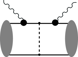
Figure 12: One Feynman diagram which is of a higher order in the chiral expansion than we consider here, but must be included in the calculation of the $\gamma$d amplitude if $T_{\gamma d}$ is to be exactly gauge invariant. The shaded blobs represent deuteron vertex functions. The small dots are vertices from the leading-order $\pi N$ Lagrangian, ${\cal L}^{(0)}$, while the larger ones are vertices from ${\cal L}^{(1)}$.

These difficulties stand in contrast to the EFT($\not\!\pi$) calculations of Refs. [29], which recover the $\gamma$d Thomson limit and also reproduce the 49 MeV Illionis data. In the nomenclature of Refs. [29, 30] our calculation of $\gamma$d scattering is valid in “Regime II”: the kinematic domain where $\omega$ is of order the deuteron binding momentum: $\omega\sim\gamma\equiv\sqrt{MB}$. The Thomson limit for $\gamma$d scattering emerges in a different regime: “Regime I” , which corresponds to photon energies of order the deuteron binding energy, i.e. $\omega\sim B$.

We now repeat the argument of Ref. [30] in order to shed some light on how the $\gamma$d Thomson limit emerges in Regime I. There the leading diagrams for Compton scattering on deuterium are shown in Fig. 13. The expressions for the operators to be sandwiched between deuteron wave functions can be written (in the $\gamma$d c.m. frame):

$$\hat{O}^{(a)} = -\frac{e^{2}}{M}{\vec{\epsilon}\,^{\prime}}\cdot{\vec{\epsilon}};$$

$$\hat{O}^{(b)} = -\frac{e^{2}}{M^{2}}{\vec{\epsilon}\,^{\prime}}\cdot{\vec{p}}\frac{1}{\omega+{\textstyle{\omega^{2}\over 2M_{d}}}-B-\frac{{\vec{p}}^{\,2}}{M}}{\vec{\epsilon}}\cdot{\vec{p}}$$

$$\hat{O}^{(c)} = -\frac{e^{2}}{M^{2}}{\vec{\epsilon}}\cdot{\vec{p}}\frac{1}{{\textstyle{\omega^{2}\over 2M_{d}}}-B-\omega-\frac{({\vec{p}}-2\vec{k}_{+})^{2}}{2M}-\frac{{{\vec{p}}\,}^{2}}{2M}}{\vec{\epsilon}\,^{\prime}}\cdot{\vec{p}};$$ (46)

where we have omitted the M1 piece of the $\gamma NN$ vertex, as well as the portions of the E1 vertex proportional to ${\vec{k}}$, the photon momentum, since they are irrelevant to what follows. Note that nucleon recoil is included in the intermediate-state propagators here, i.e. they are not the standard heavy-baryon propagators, which would give only $1/\omega$ and $-1/\omega$ respectively.

Figure 13: Leading diagrams in Regime I for $\gamma$d scattering in EFT($\not\!\pi$).

Evaluation of the operators $\hat{O}^{(a)}$–$\hat{O}^{(c)}$ between “zero-range” deuteron wave functions

$$\psi(\vec{r}^{\,})=\sqrt{\frac{\gamma}{2\pi}}\frac{e^{-\gamma r}}{r},$$ (47)

yields the result [30]:

$$-\frac{e^{2}}{M}\left[\frac{4\gamma}{|\vec{q}^{\,}|}\arctan\left(\frac{|\vec{q}^{\,}|}{4\gamma}\right)+\frac{2\gamma^{4}}{3M^{2}\omega^{2}}\left\{2-\left(1-\frac{M\omega}{\gamma^{2}}-i\eta\right)^{3/2}-\left(1+\frac{M\omega}{\gamma^{2}}\right)^{3/2}\right\}\right]{\vec{\epsilon}\,^{\prime}}\cdot{\vec{\epsilon}},$$ (48)

with $|{\vec{q}}^{\,}|=\sqrt{2}\omega(1-\cos(\theta))$. (Pieces of the graphs in Fig. 13 down by a relative factor of $\omega/M$ must be omitted in order to obtain (48).) Taking the limit $\omega\rightarrow 0$ here yields the Thomson limit for Compton scattering on the deuteron:

$$T_{\gamma d}(\omega=0)=-\frac{e^{2}}{2M}{\vec{\epsilon}\,^{\prime}}\cdot{\vec{\epsilon}},$$ (49)

up to corrections due to deuteron binding, which are very small, being of order $B/(2M)$.

An important feature of this argument is that in EFT($\not\!\pi$) an exact accounting of effects due to the scale $\sqrt{M\omega}$ can be performed. They produce the second term in Eq. (48). As discussed in Ref. [15], such contributions are higher order in our power counting, since if $\omega\sim m_{\pi}$ they involve high relative momenta inside deuterium, which means that the deuteron wave function only enters the integral in regions where it is very small. Thus our calculation includes only the first term in Eq. (48). However, as $\omega\rightarrow{\textstyle{m_{\pi}^{2}\over M}}$ effects from the scale $\sqrt{M\omega}$ become important, since the deuteron wave function is no longer being evaluated at a high scale. So, a power counting which regards only diagram (a) as the leading-order result, as ours does, is not correct in this very-low-energy regime. Indeed, with diagram (a) alone included, the amplitude (49) is not recovered: a threshold cross section that is a factor of $M_{d}/M$ too large results. This is the source of our difficulty in reproducing lower-energy deuteron Compton data.

In the absence of a full accounting of the effects of this scale in $\chi$PT we can only treat more carefully those diagrams which seem to become enhanced for $\omega\sim\frac{m_{\pi}^{2}}{M}$. Of these diagrams the argument of Ref. [30] indicates that the most important are 13(b) and 13(c). Provided we are in the regime $\omega\gg B$, we can evaluate these diagrams keeping only the contributions from the pole at $|{\vec{p}}^{\,}|^{2}=M\omega$. Neglecting the effects of analytic structure at $p\sim\gamma$ and $p\sim\omega$ , which are suppressed by $B/\omega$ and $\omega/M$ respectively, we get, for 13(b):

$$T_{s-channel\,\,pole}=\frac{i\pi e^{2}}{2\sqrt{M\omega}M}\int\frac{d^{3}p}{(2\pi)^{3}}\,\,\psi^{*}\left({\vec{p}}-{\textstyle{1\over 2}}{{\vec{k}}^{\,\prime}}\right)\,\,{\vec{\epsilon}\,^{\prime}}\cdot{\vec{p}}\,\,\delta\left(|{\vec{p}}\;|-\sqrt{M\omega}\right)\,\,{\vec{\epsilon}}\cdot{\vec{p}}\,\,\psi\left({\vec{p}}-{\textstyle{1\over 2}}{\vec{k}}\right),$$ (50)

If we assume, for the time being, that $\psi$ has only S-wave components, and again use the hierarchy $\sqrt{\omega M}\gg\omega=|{\vec{k}}^{\,}|=|{{\vec{k}}^{\,\prime}}|$ then:

$$T_{s-channel\,\,pole}=\frac{ie^{2}}{12M\pi}\,(M\omega)^{3/2}\left|\psi\left(\sqrt{M\omega}\right)\right|^{2}\,{\vec{\epsilon}\,^{\prime}}\cdot{\vec{\epsilon}}.$$ (51)

Note that in the strict HB$\chi$PT expansion the imaginary part of the $\gamma$d amplitude is zero to all orders, provided that $\omega<m_{\pi}$. However, Eq. (51) provides a leading effect in ${\rm Im}(T)$ once we resum the recoil effects in the baryon propagator. Of course, a number of other mechanisms contribute to ${\rm Im}(T)$, but Eq. (51) does allow us to estimate its size. It indicates that the imaginary part has little effect on elastic $\gamma$d cross sections at the energies considered in this work.

An expression similar to Eq. (51), but with a result that is ultimately purely real, exists for diagram 13(c):

$$T_{u-channel\,\,pole}=\frac{e^{2}}{12M\pi}\,(M\omega)^{3/2}\left|\psi\left(\sqrt{M\omega}\right)\right|^{2}\,{\vec{\epsilon}\,^{\prime}}\cdot{\vec{\epsilon}}.$$ (52)

Inserting the Fourier transform of Eq. (47) into Eqs. (51) and (52) we recover a result that agrees with Eq. (48), as long as $\omega\gg B$. More generally, if $\omega\sim{\textstyle{m_{\pi}^{2}\over M}}$, and so $\psi$ is not small, we see that 13(b) and (c) are numerically as important as the Thomson term 13(a) .

And yet including diagrams 13(b) and (c) at the same order as the Thomson term 13(a) violates the strict HB$\chi$PT power counting. It amounts to resuming an infinite set of recoil corrections for the two-nucleon propagator, all of which are higher-order in the original power counting. Below we refer to this as the “very-low-energy resummation”. To assess the impact of this resummation which enhances diagrams 13(b) and (c) in the region $\omega\sim m_{\pi}^{2}/M$ we evaluated these graphs numerically using the full expression (50), together with its crossed counterpart. Diagram 13(c) proves to be the more important of the two, since it can interfere destructively with the result for diagram 13(a), provided that $|\psi(\sqrt{M\omega})|^{2}$ does not completely suppress its contribution. Ultimately it reduces the cross sections substantially at 49 MeV, but has little impact on them at 95 (and even 69) MeV [15]. This last result is not surprising, in that at these higher energies $T_{s-channel\,\,pole}$ is suppressed by factors of the deuteron wave function at momenta of order $\sqrt{Mm_{\pi}}$.

It is clearly necessary to do this very-low-energy resummation when the deuteron is probed at very low photon energies: the baryons can no longer be treated as static for $\omega\,\,\raisebox{-3.44444pt}{$\stackrel{{\scriptstyle\textstyle<}}{{\sim}}$ }{\textstyle{m_{\pi}^{2}\over M}}$, the nuclear binding scale, and the Thomson limit (49) will only be recovered if recoil terms for the baryons are included in the calculation. However, arbitrarily including just 13(b) and (c) ignores the possibility that in this very-low-energy regime other diagrams may also be enhanced compared to their $\omega\sim m_{\pi}$ importance.

In fact, as emphasized in Ref. [48], getting low-energy theorems correct can be quite complicated in a theory where the photon scatters from the deuteron’s constituent nucleons and pions, just as recovering the Thomson limit for the proton can be quite difficult in a constituent quark model of proton structure [2]. As pointed out at the end of Section 2.2, for the EFT discussed here in the very-low energy region the breakdown into reducible and irreducible diagrams changes: $K_{\gamma\gamma}$ is no longer irreducible, and one needs to account for the appearance of the full two-nucleon propagator $G$ between photon absorption and emission. Working this out in detail remains an important challenge. Although it bears pointing out that once $\omega\,\,\raisebox{-3.44444pt}{$\stackrel{{\scriptstyle\textstyle<}}{{\sim}}$ }{\textstyle{m_{\pi}^{2}\over M}}$ EFT($\not\!\pi$) may be a more efficient way to calculate Compton scattering on deuterium, since at these low energies it is not necessary to include pions explicitly in the theory in order to achieve a good description of the data [29].

6.4 Fits to deuteron Compton data

Over the past decade three experimental groups have measured elastic $\gamma$d scattering. The data set includes:

1. The pioneering measurements by Lucas at Illinois, who took four data points at 49 MeV and two at 69 MeV [19]. The four 49 MeV points were taken in two different runs, and will, in principle, have uncorrelated systematic errors, therefore we choose to class these four points as from two different experiments.

2. Five measurements taken at SAL at photon energies ranging from 84–105 MeV [20]. Data over this energy range was consolidated into one energy bin, and we quote it at a lab photon energy of 94.5 MeV.

3. The very recent data set from MAX-Lab from Lund, which includes 9 points at approximately 55 MeV, and another 9 measurements at approximately 66 MeV [21].

	$E_{\gamma}$ (MeV)	Angle (deg.)	$\frac{d\sigma}{d\Omega}$ (nb/sr)	Stat. error	Syst. error
Illinois	49.0	50.0	15.56	1.42	0.58
		110.0	10.76	1.36	0.39
Illinois	49.0	75.0	11.25	0.84	0.40
		140.0	17.87	1.20	0.65
Illinois	69.0	60.0	13.40	0.65	0.52
		135.0	15.05	0.63	0.54
SAL	94.5	36.8	13.3	1.3	0.9
		62.7	13.5	0.8	0.7
		93.0	11.5	0.6	0.6
		122.6	15.7	1.1	0.8
		151.5	18.6	1.1	1.0
Lund	54.9	44.3	16.6	3.3	1.8
	54.6	44.9	16.8	4.1	1.5
	55.9	50.2	13.4	2.7	1.0
	54.6	125.0	15.7	1.5	1.3
	54.9	127.6	15.4	1.3	1.0
	55.9	131.7	15.3	2.0	1.2
	54.9	136.3	18.4	1.7	1.6
	54.6	136.8	17.2	2.0	1.4
	55.9	137.3	21.0	3.2	2.2
	65.6	44.4	18.6	2.4	1.4
	65.3	44.9	16.0	2.8	1.4
	67.0	50.3	15.2	1.8	1.2
	65.3	125.3	15.3	1.3	1.4
	65.6	127.8	16.0	1.2	1.1
	67.0	131.8	14.2	1.5	1.0
	65.6	136.5	15.1	1.7	1.3
	65.3	136.8	12.6	1.7	1.8
	67.0	137.5	15.0	2.7	1.2

Table 2: Deuteron Compton data sets from Illinois [19], SAL [20], and Lund [21]. Cross sections and angles are quoted in the lab frame for the Illinois data and the c.m. frame for the SAL and Lund data. Statistical and systematic errors are reported in nb/sr.

In Table 2 we list all of the data, including systematic and statistical errors. Note that in the table the angles and cross sections are in the center-of-mass frame for the SAL and MAX-Lab data, and in the lab frame for the Lucas data. Note also that since the higher-energy Lund data was taken at almost the same energy as the 69 MeV Illionis data in what follows we show them on the same plot, and compare them to calculations at $E_{\gamma}=67$ MeV. In the fits by which $\alpha_{N}$ and $\beta_{N}$ were determined the energies listed in Table 2 were used to calculate the values for $(d\sigma/d\Omega)_{\rm theory}$.

Figure 14: Results of the $O(Q^{4})$ best fit (including very-low-energy resummation) to the (lab and c.m. as appropriate) differential cross sections for Compton scattering on deuterium at four different lab photon energies: 49, 55, 67, and 94.5 MeV. The data are from Illinois [19] (circles), Lund [21] (diamonds) and SAL (squares) [20]. The error bars represent the quoted statistical (only) uncertainties of these measurements. The solid line is the $O(Q^{4})$ calculation with $\alpha_{N}=13.0\times 10^{-4}~{}{\rm fm}^{3}$, $\beta_{N}=-1.8\times 10^{-4}~{}{\rm fm}^{3}$ (Fit III). The gray area is the region excluded from the fit ($\omega,\sqrt{|t|}>160$ MeV). The dot-dashed line is the (parameter-free) $O(Q^{3})$ calculation.

These fits seek to minimize the $\chi^{2}$ defined in Eq. (29), where systematic errors are accounted for via a floating normalization. (In the case of the world $\gamma$d data the index $j$ of Eq. (29) runs from 1 to 5.) Minimizing this $\chi^{2}$ employing the NLO $\chi$PT deuteron wave function of Ref. [45] we find a $\chi^{2}$ per degree of freedom of 2.36, with a best-fit result of $\alpha_{N}=13.6\times 10^{-4}~{}{\rm fm}^{3}$ and $\beta_{N}=0.1\times 10^{-4}~{}{\rm fm}^{3}$. This fit, already shown in Fig. 10, has a rather high $\chi^{2}$. Examining the cross sections resulting from this calculation shows that the main contributions to the $\chi^{2}$ come from the two backward-angle SAL points, and from the fact that the calculation severely over-predicts the 49 MeV Illinois data. Both of these problems are associated with the regime of validity of our calculation, which is valid for $\omega\sim m_{\pi}$, but breaks down both at lower energies $\sim m_{\pi}^{2}/M$, where some of the Illinois data were taken, and for values of $\sqrt{|t|}$ of order the Delta-nucleon mass difference, where the last two SAL points occur.

In order to deal with this difficulty at higher $\sqrt{|t|}$ we followed the same procedure as employed above for the proton data and eliminated points with $\omega,\sqrt{|t|}>160$ MeV from the minimization. This excludes the last two SAL points from the fit, because our theory apparently does not include all the physics necessary to describe these points accurately. Refitting then reduces the $\chi^{2}/{\rm d.o.f.}$ to 1.95, with best-fit values of $\alpha_{N}$ and $\beta_{N}$ equal to $15.4\times 10^{-4}~{}{\rm fm}^{3}$ and $-2.3\times 10^{-4}~{}{\rm fm}^{3}$ respectively.

While the restriction on the kinematic range of the fit affects the central values of $\alpha_{N}$ and $\beta_{N}$ it does not reduce the $\chi^{2}$ markedly, because the agreement with the 49 MeV data is still poor. In contrast, implementing the very-low-energy resummation (Sec. 6.3) and then refitting produces a marked improvement in our description of the data—especially at energies around 50 MeV. The $\chi^{2}/{\rm d.o.f}$ is reduced to 1.33, and the best-fit values for nucleon electric and magnetic polarizabilities are now $13.0$ and $-1.8$ respectively. This fit (Fit III) is presented in Fig. 14, and is clearly quite good; especially when one considers that the overall normalization of each set can be adjusted within their quoted systematic uncertainty. Omitting the 49 MeV Illinois data from the fit entirely results in similar central values for $\alpha_{N}$ and $\beta_{N}$, but with a larger statistical uncertainty.

Figure 15: Results of the $O(Q^{4})$ calculation at four different lab photon energies: 49, 55, 67, and 94.5 MeV. Data as in Fig. 10. The solid line is the $O(Q^{4})$ result (including very-low-energy resummation) with $\alpha_{N}=11.5\times 10^{-4}~{}{\rm fm}^{3}$ and $\beta_{N}=0.3\times 10^{-4}~{}{\rm fm}^{3}$ (Fit IV), while the dot-dashed line is the (parameter-free) $O(Q^{3})$ calculation.

Finally, the constraint $\omega,\sqrt{|t|}<160$ MeV can be modified to $\omega,\sqrt{|t|}<200$ MeV, which allows all of the data to be fitted. The results of that fit are shown in Fig. 15, and are presented in Table 3, together with the three other fits discussed so far.

The numbers differ from those given in our earlier publication [16] for two reasons. First, there we mistakenly fitted the SAL data at a c.m. energy of 95 MeV, whereas here we have done so at a lab energy of 94.5 MeV. This causes a relatively small change in the results for most quantities in Table 3, but it does increase the central value for $\alpha_{N}$ obtained with the Nijm93 wave function by $1.0\times 10^{-4}~{}{\rm fm}^{3}$ over the value quoted in Ref. [16]. A larger effect occurs because there was an error in the program used to generate the $O(Q^{4})$ results presented for $\gamma$d scattering in Ref. [16]. The $\gamma N$ amplitude used there was missing a factor of $i$ in its spin-dependent parts. This affects the $O(Q^{3})$ results by less than 1%. However, at $O(Q^{4})$ the omission of this factor modifies the interference between the $A_{3}$–$A_{6}$ pieces of the single-nucleon amplitude and the $O(Q^{4})$ two-body currents. Correcting this mistake increases the predicted cross sections by about 10-15% with respect to those published in Ref. [16], and those which appeared in the first version of this paper [56]. We emphasize that this mistake was not made in the $\gamma$p calculation reported in Ref. [16] and discussed in Secs. 3 and 4 above.

Fit	Wave	Very-low-energy	$\omega,\sqrt{|t|}$	$\alpha_{N}$	$\beta_{N}$	$\chi^{2}$/d.o.f.
	function	resummation?	below	$(10^{-4}~{}{\rm fm}^{3})$	$(10^{-4}~{}{\rm fm}^{3})$
I	NLO $\chi$PT	No	$200$ MeV	13.6	$0.1$	2.36
II	NLO $\chi$PT	No	$160$ MeV	15.4	$-2.3$	1.95
III	NLO $\chi$PT	Yes	$160$ MeV	13.0	$-1.8$	1.33
IV	NLO $\chi$PT	Yes	$200$ MeV	11.5	$0.3$	1.69
V	Nijm93	Yes	$200$ MeV	16.9	$-2.7$	2.87

Table 3: Results of our different $O(Q^{4})$ EFT extractions of isoscalar nucleon polarizabilities from low-energy coherent $\gamma$d scattering data.

As discussed above, cross sections depend on the choice of deuteron wave function at the 10-20% level. This change in the $\gamma$d cross section has a significant effect on the extraction of $\alpha_{N}$ and $\beta_{N}$. Changing only the wave function yields the difference between Fit IV and Fit V in Table 3. The high $\chi^{2}$ of Fit V is again due to a failure to reproduce the 49 MeV data—this time even when the very-low-energy resummation of Section 6.3 is performed. While the Nijm93 wave function is not consistent with $\chi$PT, it does have the correct long-distance behavior. The differences we see are therefore a consequence of the different short-range behavior of the Nijm93 and NLO $\chi$PT $NN$ potentials. As such they should be renormalized by $\gamma NN\rightarrow\gamma NN$ contact operators. However, Weinberg power counting predicts that the appropriate operators do not appear until (at least) $O(Q^{5})$. Thus, the degree of variability between the results with the NLO $\chi$PT and Nijm93 wave functions could be said to be inconsistent with Weinberg power counting. Indeed, it may be necessary to modify the Weinberg power counting so that such contact operators appear at a lower order than is indicated by naive dimensional analysis. Further understanding of this issue is clearly crucial to the use of $\chi$PT as an accurate calculational tool for low-energy reactions on deuterium, but lies beyond the scope of this paper. Here we adopt the conservative strategy of assigning a theoretical error which encompasses both the Nijm93 and NLO $\chi$PT results.

Figure 16: Allowed regions (at the 1-$\sigma$ level) for isoscalar nucleon electric and magnetic polarizabilities (in $10^{-4}\,{\rm fm}^{3}$) resulting from different $O(Q^{4})$ EFT fits to low-energy data. In the order the fits are listed in Table 3 the constraints are: fit I (short-dashed, red); fit II (medium-dashed, orange); fit III (solid black); fit IV (long-dashed, green); fit V (dot-dashed, blue). For comparison, the Baldin sum-rule constraint found by averaging the proton and neutron results of Ref. [57] is shown as the gray shaded band.

The $\chi^{2}$ contours for the five fits of Table 3 are shown in Fig. 16, with the “best fit” EFT (Fit III) giving the 1-sigma region bounded by the solid black line. Putting these results together we conclude that our central values, and error bars, for the isoscalar nucleon polarizabilities are:

$$\alpha_{N} = (13.0\pm 1.9)_{-1.5}^{+3.9}\times 10^{-4}\,{\rm fm}^{3},$$

$$\beta_{N} = (-1.8\pm 1.9)_{-0.9}^{+2.1}\times 10^{-4}\,{\rm fm}^{3}.$$ (53)

The errors inside the brackets are statistical, and those outside reflect the arbitrariness as to which data are included, and which deuteron wave function is employed.

The theoretical error should also include a component from higher-order ($O(Q^{5})$ and above) pieces of the $\gamma NN$ kernel. A number of these are taken into account in the sophisticated potential-model calculations of Refs. [26, 27, 28]. Including them in the calculation will alter the central values, although the theoretical error arising from wave-function dependence and the variation in the kinematical cuts we impose is large enough that we expect it encompasses the impact of higher-order terms in the kernel.

Combining Eqs. (30) and (53) we see that a wide range of neutron polarizabilities is consistent with a model-independent analysis of the current low-energy $\gamma$p and coherent $\gamma$d data. However, there is clear statistical evidence in these data sets for $\alpha_{n}$ being significantly larger than $\beta_{n}$: $\beta_{n}$ is consistent with zero within our large error bars. Also, the results presented here provide no evidence for significant isovector components in $\alpha$ and $\beta$, in contrast to some previous results in the literature (see, e.g. Ref. [20]).

6.5 Other techniques for measuring $\alpha_{n}$

A dispersion sum rule—analogous to the Baldin sum rule for the proton—that relates the sum of isoscalar nucleon electric and magnetic polarizabilities to an integral of the deuteron photo-absorption cross section can be derived, if one assumes that the single-nucleon contribution dominates the deuteron photoabsorption cross section. Using this sum rule, and subtracting their result for $\alpha_{p}+\beta_{p}$, the authors of Ref. [57] found:

$$\alpha_{n}+\beta_{n}=(14.40\pm 0.66)\times 10^{-4}\,{\rm fm}^{3}.$$ (54)

This result is not consistent with our “best fit” result if only statistical errors are considered, but if one includes the theoretical errors in Eq. (53) there is no discrepancy. Moreover, the theoretical error on the sum rule associated with assuming that the free neutron photoabsorption cross section can be found by taking the difference of deuteron and proton data is not clear.

A more sophisticated evaluation of the neutron photoabsorption integral that uses the neutron multipoles of Ref. [58] at low energy, together with experimental deuteron and proton photoabsorption cross sections at intermediate energies, and Regge phenomenology at energies above 1.5 GeV yields [27]:

$$\alpha_{n}+\beta_{n}=(15.2\pm 0.5)\times 10^{-4}\,{\rm fm}^{3}.$$ (55)

The theoretical error given in Ref. [27] is arrived at by employing different neutron pion photoproduction multipoles in the sum-rule integrand for the region up to $\omega=500$ MeV. However, the theoretical errors from the multipole analyses themselves seem not to have been assessed. Further, the extent to which the theoretical error in the high-energy part of the amplitude affects the final result is not clear to us.

Most direct information on $\alpha_{n}$ has been obtained by scattering neutrons on a heavy nucleus and examining the cross section as a function of energy. Controversy remains over what result this technique gives for $\alpha_{n}$. In Ref. [59] the value 

$$\alpha_{n}=(12.6\pm 1.5\pm 2.0)\times 10^{-4}\,{\rm fm}^{3}$$ (56)

was obtained, which disagrees considerably with the result of the experiment of Ref. [62],

$$\alpha_{n}=(0.6\pm 5.0)\times 10^{-4}\,{\rm fm}^{3}.$$ (57)

Recent data from MAMI [24] exist for quasi-free $\gamma d\rightarrow\gamma pn$ in the 200 to 400 MeV range. These experiments update the pioneering work of Ref. [22], which was only able to set an upper bound on $\alpha_{n}$ from this process. Ref. [24] reports the measurement of the reaction $\gamma d\rightarrow\gamma pn$ for laboratory photon scattering angles of 136.2 degrees, and then uses a theoretical model to extract:

$$\alpha_{n}-\beta_{n}=(9.8\pm 3.6~{}({\rm stat.}))^{+2.1}_{-1.1}~{}({\rm syst.})\pm 2.2({\rm model})\times 10^{-4}~{}{\rm fm}^{3},$$ (58)

from their data. This refines the constraint on $\alpha_{n}-\beta_{n}$ obtained somewhat earlier at SAL, where quasi-free Compton deuteron breakup was measured in the narrower range between 236 and 260 MeV of photon energy and analyzed using the same theoretical model [23]. The result (58) is consistent with the broad range for $\alpha_{n}-\beta_{n}$ indicated by our analysis of the low-energy coherent $\gamma$p and $\gamma$d data.

7 Conclusion

Starting from the most general Lagrangian that includes pions and nucleons and shares the global symmetries of QCD, we have calculated the amplitude for Compton scattering on the deuteron in $\chi$PT up to $O(Q^{4})$. This amplitude consists of one- and two-nucleon pieces averaged over incoming and outgoing deuteron wave functions. Both the $\gamma NN$ kernel and the deuteron wave function were obtained from the same Lagrangian, with a consistent set of parameters.

The one-nucleon piece of the $\gamma NN$ kernel is the same as the amplitude for Compton scattering on a nucleon. This was calculated to $O(Q^{4})$ in the usual $\chi$PT power counting in Ref. [12]. That calculation contains four unknown parameters, which correspond to short-range contributions to electric and magnetic polarizabilities of the proton and the neutron. In this work we fitted the world’s low-energy proton data [17, 18] and determined the two proton polarizabilities, obtaining values similar to the Particle Data Group’s [50].

We also calculated the two-nucleon kernel to the same order, using the power counting suggested by Weinberg [13]. It consists of various one-pion-exchange contributions with no unknown parameters. Finally, we used deuteron wave functions fully determined in the same approach [45]. To this order, the deuteron amplitude is sensitive only to the two isoscalar combinations of the nucleon electric and magnetic polarizabilities. From the $\gamma$d amplitude we calculated the differential cross section and compared it with deuteron data at various photon energies below 100 MeV [19, 20, 21]. A good fit was obtained and we extracted from it results for the two isoscalar polarizabilities, which, together with our results for proton polarizabilities, allow an extraction of neutron polarizabilities. Various theoretical systematic uncertainties were studied.

As pointed out in the Introduction, various sophisticated calculations of this process exist using potential models [26, 27, 28]. Two of the distinctive features of our work are the use of a consistent $\chi$PT framework throughout, and the fact that we employ only low-energy data. We have used only data that we believe—on the basis of statistical tests—falls within the domain of the EFT. We find that a wide range of neutron polarizabilities is consistent with a model-independent analysis of this $\gamma$p and coherent $\gamma$d data. Narrower ranges for the neutron polarizabilities can be obtained from the data at the expense of additional assumptions which introduce model dependence.

The potential-model calculations of Refs. [26, 27, 28] can be broken up into one- and two-body kernels and wave functions in the same way ours can. However, typically the different pieces are not calculated using a fully consistent field theory. The wave function is calculated from a phenomenological potential model that does not include, e.g., the two-pion exchange required by quantum field theory, but instead employs various single-meson exchanges. The best calculations strive for consistency of the $\gamma NN$ kernel with the two-nucleon potential by including in it the same mesons with the same form factors. This also leads to a gauge-invariant $\gamma$d amplitude if the necessary photon seagull diagrams are included [27]. Meanwhile the $\gamma N$ piece of the $\gamma NN$ kernel in Refs. [26, 27, 28] includes a polynomical expansion of the $\gamma$N amplitude. They thus omit pieces of the $\gamma N$ amplitude which are not analytic in the photon energy [15]. On the other hand, the model calculations include a number of contributions that in our framework appear only at higher order. There is qualitative, but not quantiative, agreement between the different calculations and also between these potential-model calculations and the $\chi$PT calculation reported on here.

This is perhaps not surprising, since the potential-model calculations can be understood as various approximations to effective field theory. Indeed, it is one of the features of EFT that models which do not badly violate symmetries of QCD should—at low energies—reduce to the EFT with a particular choice of low-energy constants. (This choice may, or may not, agree with the choice that is made by QCD.) Contrary to what is apparently a common misconception in the literature, there are no more unknown parameters in our calculation than in these potential-model calculations.

Various previous extractions of polarizabilities have also differed from ours in the emphasis given to low-energy data. Frequently the Baldin sum rule [51]—which relies on certain (reasonable) assumptions about the behavior of QCD amplitudes at higher energies, and on model-based interpolation of data— is used. Our results are consistent with the Baldin sum-rule results for $\alpha_{p}+\beta_{p}$ [18], but do not rely on them. In addition, our results are consistent, within error bars, with the recent extraction of $\alpha_{N}\pm\beta_{N}$ from the Lund data using the detailed model of Levchuk and L’vov [21, 27]. (But see also the values found using the data of Refs. [19, 20] and this model [20, 27].).

There are several ways to improve our present calculation. First, a complete treatment of the very-low-energy region would allow inclusion of low-energy data that could be measured at HI$\gamma$S [63]. Second, one would like to systematically go to $O(Q^{5})$ and higher in the present energy regime. The significant dependence of our results for $\alpha_{N}$ and, to a lesser extent, $\beta_{N}$, on the choice of deuteron wave function also warrants further work. It could have important implications for the formulation of a fully-consistent nuclear effective theory.

A promising future direction is the addition of an explicit Delta-isobar field, which would allow us to address higher-energy data using the same EFT philosophy employed here. A recent breakthrough in power counting has facilitated the use of $\chi$PT for reaction energies up to the Delta peak, in particular in the case of Compton scattering on the nucleon [35]. Compton scattering on the deuteron has very recently been tackled along these lines, and it seems that the inclusion of an explicit Delta degree of freedom ameliorates the diffculties we had in reproducing the backward-angle SAL data [64].

Finally, there is, in principle, no obstacle to carrying out EFT calculations for the quasi-free process $\gamma d\rightarrow\gamma np$, and including the existing data [22, 23, 24] in the extraction of neutron polarizabilities. We hope that these various improvements will eventually lead to the use of EFT as a model-independent framework within which nucleon polarizabilities can be extracted from experimental data gathered in a number of different reactions.

Appendix A Third-order loop amplitude

The third-order one-nucleon loop graphs give the following amplitude in a general frame. The notation ${\bf t}_{i}$ is used for the tensor structures which multiply the amplitudes $A_{i}$ of Eq. (20); for example ${\bf t}_{1}={\vec{\epsilon}\,^{\prime}}\cdot{\vec{\epsilon}}$.

$$T_{i} = {g_{A}^{2}e^{2}\over 2f_{\pi}^{2}}({\bf t}_{1}+{\bf t}_{3})J_{0}[{\overline{\omega}},m_{\pi}^{2}]+\hbox{crossed}$$

$$T_{ii} = -{g_{A}^{2}e^{2}\over 2f_{\pi}^{2}}({\bf t}_{1}+{\bf t}_{3})\int_{0}^{1}\!dx\bigl{(}J_{0}[{\overline{\omega}}-x\omega,m_{\pi}^{2}]+J_{0}[{\overline{\omega}}-x\omega^{\prime},m_{\pi}^{2}]\bigr{)}+\hbox{crossed}$$

$$T_{iii} = {g_{A}^{2}e^{2}\over 2f_{\pi}^{2}}\int_{0}^{1}\!dy\int_{0}^{1-y}\!dx\Bigl{[}(d+1){\bf t}_{1}J_{0}[\tilde{\omega},m_{\pi}^{2}-xyt]$$

$$+\Bigl{(}2(x+y-(d+3)xy)\omega\omega^{\prime}{\bf t}_{2}-2V(x,y){\bf t}_{1}-2(1\!-\!x\!-\!y)\omega\omega^{\prime}{\bf t}_{4}\Bigr{)}J_{0}^{\prime}[\tilde{\omega},m_{\pi}^{2}-xyt]$$

$$\qquad+4\omega\omega^{\prime}xy\Bigl{(}V(x,y){\bf t}_{2}+(1\!-\!x\!-\!y)\omega\omega^{\prime}{\bf t}_{7}\Bigr{)}J_{0}^{\prime\prime}[\tilde{\omega},m_{\pi}^{2}-xyt]$$

$$\qquad\qquad+2\Bigl{(}yi\vec{\sigma}\cdot({\vec{\epsilon}\,^{\prime}}\times\vec{q}){\vec{\epsilon}}\cdot{{\vec{k}}^{\,\prime}}+xi\vec{\sigma}\cdot({\vec{\epsilon}}\times\vec{q}){\vec{\epsilon}\,^{\prime}}\cdot{\vec{k}}\Bigr{)}J_{0}^{\prime}[\tilde{\omega},m_{\pi}^{2}-xyt]\Bigr{]}+\hbox{crossed}$$

$$T_{iv} = -{g_{A}^{2}e^{2}\over 2f_{\pi}^{2}}{\bf t}_{1}\int_{0}^{1}\!dx\Bigl{[}(d-1)J_{0}[(x-{\textstyle{1\over 2}})\delta\omega,m_{\pi}^{2}-x(1-x)t]$$ (59)

$$\qquad\qquad\qquad-2x(1-x)(t-\delta\omega^{2})J_{0}^{\prime}[(x-{\textstyle{1\over 2}})\delta\omega,m_{\pi}^{2}-x(1-x)t]\Bigr{]}$$

where ${\overline{\omega}}=(\omega+\omega^{\prime})/2$, $\tilde{\omega}=({\overline{\omega}}-x\omega-y\omega^{\prime})$, $\vec{q}={\vec{k}}-{{\vec{k}}^{\,\prime}}$, $t=(k^{\prime}-k)^{2}=2\omega\omega^{\prime}(\cos\theta-1)$, $\delta\omega=\omega-\omega^{\prime}$. The integrals $J_{0}[\omega,m_{\pi}^{2}]$, $J_{2}[\omega,m_{\pi}^{2}]$ and $\Delta_{\pi}[m_{\pi}^{2}]$ have their usual meanings [9], prime denotes differentiation with respect to $m_{\pi}^{2}$, and

$$V(x,y)=\tilde{\omega}^{2}+\omega\omega^{\prime}-{\overline{\omega}}^{2}+{\textstyle{1\over 2}}t(1-x-y+2xy).$$ (60)

We have also introduced an extra tensor structure: ${\bf t}_{7}=\vec{\sigma}\cdot(\hat{k^{\prime}}\times\hat{k}){\vec{\epsilon}\,^{\prime}}\cdot\hat{k}\,{\vec{\epsilon}}\cdot\hat{k^{\prime}}.$ This is not independent; ${\bf t}_{7}=\sin^{2}\theta{\bf t}_{3}+\cos\theta{\bf t}_{5}-{\bf t}_{6}$, but as it arises naturally in the calculations—and enters at too high an order in $\omega$ to affect the polarizabilities—it is a useful notation.

The notation “+ crossed” means that to every term is added another with ${\vec{\epsilon}}\leftrightarrow{\vec{\epsilon}\,^{\prime}}$, ${\vec{k}}\leftrightarrow-{{\vec{k}}^{\,\prime}}$ and $\omega\leftrightarrow-\omega^{\prime}$. Since the ${\bf t}_{i}$ are all either symmetric or antisymmetric under this transformation, the net effect is to add a term with $\omega\leftrightarrow-\omega^{\prime}$ to the coefficients of ${\bf t}_{1}$ and ${\bf t}_{2}$, and subtract such a term from the coefficients of ${\bf t}_{3}-{\bf t}_{7}$.

In HB$\chi$PT the difference in photon energies, $\delta\omega$, is of order $Q^{2}/M$ . Thus for a fourth-order calculation only the expansion to first order in $\delta\omega$ is required. This gives the following amplitudes

$$T_{i} = {g_{A}^{2}e^{2}\over 2f_{\pi}^{2}}({\bf t}_{1}+{\bf t}_{3})J_{0}[{\overline{\omega}},m_{\pi}^{2}]+\hbox{crossed}$$

$$T_{ii} = -{g_{A}^{2}e^{2}\over f_{\pi}^{2}}({\bf t}_{1}+{\bf t}_{3})\int_{0}^{1}\!dxJ_{0}[x{\overline{\omega}},m_{\pi}^{2}]+\hbox{crossed}$$

$$T_{iii} = {g_{A}^{2}e^{2}\over 2f_{\pi}^{2}}\int_{0}^{1}\!dy\int_{0}^{1-y}\!dx\Bigl{\{}(d+1){\bf t}_{1}J_{0}[\tilde{\omega},m_{\pi}^{2}-xyt]$$

$$\qquad\qquad+\Bigl{(}2(x+y-(d+3)xy){\overline{\omega}}^{2}{\bf t}_{2}-2V(x,y){\bf t}_{1}$$

$$\qquad\qquad\qquad\qquad\qquad-(x+y){\overline{\omega}}^{2}({\bf t}_{6}-{\bf t}_{5})-2(1\!-\!x\!-\!y){\overline{\omega}}^{2}{\bf t}_{4}\Bigr{)}J_{0}^{\prime}[\tilde{\omega},m_{\pi}^{2}-xyt]$$

$$\qquad\qquad+{\textstyle{1\over 2}}(x-y)^{2}\delta{\overline{\omega}}\Bigl{(}i\vec{\sigma}\cdot({\vec{\epsilon}\,^{\prime}}\times\vec{q}){\vec{\epsilon}}\cdot{{\vec{k}}^{\,\prime}}-i\vec{\sigma}\cdot({\vec{\epsilon}}\times\vec{q}){\vec{\epsilon}\,^{\prime}}\cdot{\vec{k}}\Bigr{)}{\partial J_{0}^{\prime}[\tilde{\omega},m_{\pi}^{2}-xyt]\over\partial\tilde{\omega}}$$

$$\qquad\qquad\qquad+4xyw^{2}\bigl{(}V(x,y){\bf t}_{2}+(1\!-\!x\!-\!y){\overline{\omega}}^{2}{\bf t}_{7}\bigr{)}J_{0}^{\prime\prime}[\tilde{\omega},m_{\pi}^{2}-xyt]\Bigr{\}}+\hbox{crossed}$$

$$T_{iv} = -{g_{A}^{2}e^{2}\over 2f_{\pi}^{2}}{\bf t}_{1}\int_{0}^{1}\!dx\Bigl{[}(d-1)J_{0}[0,m_{\pi}^{2}-x(1-x)t]$$ (61)

$$\qquad\qquad\qquad\qquad\qquad\qquad-2x(1-x)\,t\,J_{0}^{\prime}[0,m_{\pi}^{2}-x(1-x)t]\Bigr{]}$$

where $\tilde{\omega}=(1\!-\!x\!-\!y){\overline{\omega}}$, and

$$V(x,y)=\tilde{\omega}^{2}+{\textstyle{1\over 2}}t(1-x-y+2xy).$$ (62)

There is only one term proportional to $\delta\omega$ (in $T_{iii}$), and this cancels against a piece from the fourth-order amplitude (see below).

Appendix B Fourth-order loop amplitude

The full amplitude in the Breit frame for diagrams 2a-2s can be obtained from Ref. [12]. In a general frame, there are, in addition to the Breit frame terms, contributions containing $\vec{p}_{+}$, the average of the incoming and outgoing nucleon momenta. It is useful to define the following tensor structures

$${\bf t}_{2}^{\prime} = {\vec{\epsilon}\,^{\prime}}\cdot\vec{p}_{+}\;{\vec{\epsilon}}\cdot{{\vec{k}}^{\,\prime}}+{\vec{\epsilon}}\cdot\vec{p}_{+}\;{\vec{\epsilon}\,^{\prime}}\cdot{\vec{k}}$$

$${\bf t}_{4}^{\prime} = i\vec{\sigma}\cdot(\vec{p}_{+}\times\vec{q})\;{\vec{\epsilon}\,^{\prime}}\cdot{\vec{\epsilon}}$$

$${\bf t}_{5}^{\prime} = i\vec{\sigma}\cdot({\vec{\epsilon}\,^{\prime}}\times{\vec{k}})\;\vec{p}_{+}\cdot{\vec{\epsilon}}-i\vec{\sigma}\cdot({\vec{\epsilon}}\times{{\vec{k}}^{\,\prime}})\;\vec{p}_{+}\cdot{\vec{\epsilon}\,^{\prime}}$$

$${\bf t}_{6}^{\prime} = i\vec{\sigma}\cdot({\vec{\epsilon}\,^{\prime}}\times{{\vec{k}}^{\,\prime}})\;\vec{p}_{+}\cdot{\vec{\epsilon}}-i\vec{\sigma}\cdot({\vec{\epsilon}}\times{\vec{k}})\;\vec{p}_{+}\cdot{\vec{\epsilon}\,^{\prime}}$$

$${\bf t}_{56}^{\prime} = i\vec{\sigma}\cdot({\vec{\epsilon}\,^{\prime}}\times\vec{p}_{+})\;{{\vec{k}}^{\,\prime}}\cdot{\vec{\epsilon}}-i\vec{\sigma}\cdot({\vec{\epsilon}}\times\vec{p}_{+})\;{\vec{k}}\cdot{\vec{\epsilon}\,^{\prime}}$$

$${\bf t}_{7}^{\prime} = i\vec{\sigma}\cdot(\hat{k^{\prime}}\times\hat{k})\;({\vec{\epsilon}\,^{\prime}}\cdot\vec{p}_{+}\;{\vec{\epsilon}}\cdot{{\vec{k}}^{\,\prime}}+{\vec{\epsilon}}\cdot\vec{p}_{+}\;{\vec{\epsilon}\,^{\prime}}\cdot{\vec{k}})$$

$${\bf t}_{7}^{\prime\prime} = i\vec{\sigma}\cdot(\vec{p}_{+}\times\vec{q})\;{\vec{\epsilon}\,^{\prime}}\cdot\hat{k}\;{\vec{\epsilon}}\cdot\hat{k^{\prime}}$$ (63)

The notation reflects the structures that these t’s give rise to in the center-of-mass frame. Again, not all the structures are independent, but it greatly simplifies matters to work with this set.

Diagram by diagram, the $\vec{p}_{+}$-dependent contributions are

$$T_{a} = -{g_{A}^{2}e^{2}\over 2Mf_{\pi}^{2}}({\bf t}_{1}+{\bf t}_{3})\,\vec{p}_{+}\cdot\vec{k}_{+}\,{\partial J_{0}[\omega,m_{\pi}^{2}]\over\partial\omega}+\hbox{crossed}$$

$$T_{b} = {g_{A}^{2}e^{2}\over 2Mf_{\pi}^{2}}\Bigl{(}2({\bf t}_{1}+{\bf t}_{3})\,\vec{p}_{+}\cdot\vec{k}_{+}+({\bf t}_{2}^{\prime}+{\bf t}_{5}^{\prime})\Bigr{)}\int_{0}^{1}\!dx\,x{\partial J_{0}[x\omega,m_{\pi}^{2}]\over\partial x\omega}+\hbox{crossed}$$

$$T_{f} = -{g_{A}^{2}e^{2}\over 4Mf_{\pi}^{2}}(1-\tau_{3})\,{\bf t}_{6}^{\prime}\,\omega^{-1}\int_{0}^{1}\!dxJ_{0}[x\omega,m_{\pi}^{2}]+\hbox{crossed}$$

$$T_{g} = -{g_{A}^{2}e^{2}\over 4Mf_{\pi}^{2}}(1+\tau_{3})\,{\bf t}_{6}^{\prime}\,\omega^{-1}\int_{0}^{1}\!dxJ_{0}[x\omega,m_{\pi}^{2}]+\hbox{crossed}$$

$$T_{h} = -{g_{A}^{2}e^{2}\over 2Mf_{\pi}^{2}}\int_{0}^{1}\!dy\int_{0}^{1-y}\!dx\left[(1\!-\!x\!-\!y)\vec{p}_{+}\cdot\vec{k}_{+}\left({\bf t}_{1}(d+3){\partial J_{0}[\tilde{\omega},m_{\pi}^{2}-xyt]\over\partial\tilde{\omega}}\right.\right.$$

$$\left.\left.-\Bigl{(}(x+y)\omega^{2}({\bf t}_{6}-{\bf t}_{5})+2(1\!-\!x\!-\!y)\omega^{2}{\bf t}_{4}+2V(x,y){\bf t}_{1}\right.\right.$$

$$\left.\left.\qquad\qquad\qquad\qquad\qquad\qquad+2((d+5)xy-x-y)\omega^{2}{\bf t}_{2}\Bigr{)}{\partial J_{0}^{\prime}[\tilde{\omega},m_{\pi}^{2}-xyt]\over\partial\tilde{\omega}}\right.\right.$$

$$\left.\left.+4xy\omega^{2}(V(x,y){\bf t}_{2}+(1\!-\!x\!-\!y)\omega^{2}{\bf t}_{7}){\partial J_{0}^{\prime\prime}[\tilde{\omega},m_{\pi}^{2}-xyt]\over\partial\tilde{\omega}}\right)\right.$$

$$\left.-\Bigl{(}{\textstyle{1\over 2}}((d+3)(x+y)-2){\bf t}_{2}^{\prime}-{\bf t}_{4}^{\prime}+{\bf t}_{6}^{\prime}-{\bf t}_{5}^{\prime}\Bigr{)}{\partial J_{0}[\tilde{\omega},m_{\pi}^{2}-xyt]\over\partial\tilde{\omega}}\right.$$

$$\left.+\Bigl{(}(1\!-\!x\!-\!y)(x+y)\omega^{2}{\bf t}_{7}^{\prime}-2xy\omega^{2}{\bf t}_{7}^{\prime\prime}+(x+y)V(x,y){\bf t}_{2}^{\prime}\Bigr{)}{\partial J_{0}^{\prime}[\tilde{\omega},m_{\pi}^{2}-xyt]\over\partial\tilde{\omega}}\right]$$

$$-{g_{A}^{2}e^{2}\over 4f_{\pi}^{2}}\delta\omega\int_{0}^{1}\!dy\int_{0}^{1-y}\!dx(x-y)^{2}i\bigl{(}\vec{\sigma}\cdot{\vec{\epsilon}\,^{\prime}}\times\vec{q}{\vec{\epsilon}}\cdot{{\vec{k}}^{\,\prime}}-\vec{\sigma}\cdot{\vec{\epsilon}}\times\vec{q}{\vec{\epsilon}\,^{\prime}}\cdot{\vec{k}}\bigr{)}{\partial J_{0}^{\prime}[\tilde{\omega},m_{\pi}^{2}-xyt]\over\partial\tilde{\omega}}$$

$$\kern 341.43306pt+\hbox{crossed}$$

$$T_{i} = -{g_{A}^{2}e^{2}\over Mf_{\pi}^{2}}{\bf t}_{4}^{\prime}\int_{0}^{1}\Delta_{\pi}^{\prime}[m_{\pi}^{2}-x(1-x)t]$$

$$T_{j} = {g_{A}^{2}e^{2}\over Mf_{\pi}^{2}}\int_{0}^{1}\!dy\int_{0}^{1-y}\!dx\Bigl{[}2xy{\bf t}_{7}^{\prime\prime}\omega^{2}\Delta_{\pi}^{\prime\prime}[m_{\pi}^{2}-xyt]-{\bf t}_{4}^{\prime}\Delta_{\pi}^{\prime}[m_{\pi}^{2}-xyt]+\hbox{crossed}$$

$$T_{k} = -T_{i}$$ (64)

Here we have defined $\vec{k}_{+}$ as the average of the incoming and outgoing photon momenta. The tensors ${\bf t}_{i}^{\prime}$ have the opposite crossing symmetry to the corresponding ${\bf t}_{i}$, as do the products $\vec{p}_{+}\cdot\vec{k}_{+}\,{\bf t}_{i}$.

Note that the piece in $T_{h}$ proportional to $\delta\omega$ comes from $\vec{p}_{+}\cdot\vec{q}$, and exactly cancels the piece proportional to $\delta\omega$ in the expansion to fourth order of the third-order amplitudes.

All the rest of the terms written above can alternatively be generated by a boost of the third-order Breit-frame amplitude. The transformations to do this are as follows:

$${\vec{\epsilon}} \to {\vec{\epsilon}}+\frac{{\vec{\epsilon}}\cdot\vec{p}_{+}}{M}\,\hat{k};$$

$${\vec{k}} \to {\vec{k}}-\frac{\omega}{M}\,\vec{p}_{+};$$

$$\omega \to \omega-\frac{1}{M}\vec{p}_{+}\cdot\vec{k}_{+}$$ (65)

with analogous transformations for the other photon. These boosts are odd under crossing, which accounts for the change in symmetry mentioned above. It is easily seen that the pieces of (64) proportional to $\vec{p}_{+}\cdot\vec{k}_{+}$ come from the boost of $\omega$; they are generated from the fourth-order diagrams which are just third-order diagrams with an insertion from ${\cal L}^{(1)}$ on the nucleon line. The other structures come from the boost of the vectors ${\vec{\epsilon}}$, ${\vec{k}}$, etc. Applying the boost of Eq. (65) in the third-order amplitude gives the additional terms needed to ensure equality with the result from explicit evaluation of the fourth-order diagrams in an arbitrary frame.

Appendix C Born terms

In addition to these terms arising from pion loops in a boosted frame, there are also Born terms. The complete set of Born terms corresponds exactly to the expansion in powers of $1/M$ of the result obtained from Dirac nucleons, with the vertex of an incoming photon of four-momentum $q$ being

$$\Gamma_{\mu}={\cal Z}\gamma_{\mu}+{i\kappa\over 2M}\sigma_{\mu\nu}q^{\nu},$$ (66)

as long as loop renormalizations of bare parameters such as $\kappa$ are ignored.

Born terms fall into two categories. First, there are those which do not vanish in the Breit frame,

$$T^{\rm Born}_{\rm Breit} = -{e^{2}\over 4M^{3}}\left[\Bigl{(}({\cal Z}+\kappa)^{2}(1+\cos\theta)-{\cal Z}^{2}\Bigr{)}(\cos\theta-1)\,\omega^{2}\,{\bf t}_{1}-\kappa(2{\cal Z}+\kappa)\cos\theta\,\omega^{2}\,{\bf t}_{2}\right]$$ (67)

$$\qquad\qquad\qquad+{e^{2}{\cal Z}^{2}\over 2M^{2}}E_{\rm kin}\,{\bf t}_{1}$$

where $E_{\rm kin}$ is the average kinetic energy of the nucleons. The coefficient of the nucleon kinetic energy term depends on the normalization of the Dirac spinors in the relativistic case. As shown, the normalization is $\bar{u}u=2E/(E+M)$, which is appropriate for the standard non-relativistic reduction. However, the usual covariant treatment of the Compton Born terms corresponds to the normalization $\bar{u}u=1$, in which case the last term on the right-hand side of (67) is not present.

Second, in an arbitrary frame, there are the terms generated by a boost of the LET pieces of the third-order, Breit-frame amplitude

$$T^{\rm Born}_{\rm boost} = -{e^{2}\over M^{2}\omega}{\cal Z}^{2}{\bf t}_{2}^{\prime}$$ (68)

$$- {e^{2}\over 2M^{3}}\Bigl{[}\vec{p}_{+}\cdot\vec{k}_{+}\,\Bigl{(}({\cal Z}+\kappa)^{2}({\bf t}_{3}(\cos\theta-1)+{\bf t}_{4}-{\bf t}_{5})-\kappa^{2}{\bf t}_{3}+{\cal Z}({\cal Z}+\kappa){\bf t}_{6}\Bigr{)}$$

$$+\Bigl{(}{\textstyle{1\over 2}}{\cal Z}^{2}-({\cal Z}+\kappa)^{2}\Bigr{)}{\bf t}_{4}^{\prime}+\kappa^{2}{\bf t}_{5}^{\prime}-{\cal Z}({\cal Z}+K)(1-\cos\theta){\bf t}_{6}^{\prime}+\kappa({\cal Z}+\kappa){\bf t}_{56}^{\prime}$$

$$+{\textstyle{2\over\omega^{2}}}{\cal Z}^{2}\vec{p}_{+}\cdot\vec{k}_{+}\,{\bf t}_{2}^{\prime}+2{\cal Z}^{2}(\cos\theta-1){\vec{\epsilon}}\cdot\vec{p}_{+}\,{\vec{\epsilon}\,^{\prime}}\cdot\vec{p}_{+}\Bigr{]}.$$

The first part of the ${\bf t}_{4}^{\prime}$ term comes from the Thomson term via a Wigner rotation, which is a second-order boost effect; the terms in the last line are also second-order, with the second-order boost given by

$${\vec{\epsilon}} \to {\vec{\epsilon}}+\frac{{\vec{\epsilon}}\cdot\vec{p}_{+}}{M}\,\hat{k}+\frac{(\vec{p}_{+}\cdot\hat{k})({\vec{\epsilon}}\cdot\vec{p}_{+})}{M^{2}}\,\hat{k}-\frac{{\vec{\epsilon}}\cdot\vec{p}_{+}}{2M^{2}}\,\vec{p}_{+}$$

$${\vec{k}} \to {\vec{k}}-\frac{\omega}{M}\,\vec{p}_{+}+\frac{\vec{p}_{+}\cdot{\vec{k}}}{2M^{2}}\,\vec{p}_{+}$$ (69)

The angle dependence of these Born terms is more complicated than that associated with the polarizabilities.

Appendix D $\gamma N$ kinematics in the $\gamma$d center-of-mass frame

In this appendix we consider the evaluation of the single-nucleon Compton amplitude “inside” the deuteron. This necessitates the evaluation of expectation values:

$$\langle\psi|{\bf t}_{i}^{\prime}|\psi\rangle,$$ (70)

where the ${\bf t}_{i}^{\prime}$ are the structures defined by Eq. (63), and $|\psi\rangle$ is a deuteron wave function, calculated for a deuteron at rest. In the next appendix we will explain how to correct such matrix elements for the fact that the initial-state (final-state) deuteron wave function must be calculated in a reference frame which is moving with momentum $-\vec{k}$ ($-{{\vec{k}}^{\,\prime}}$).

All ${\bf t}_{i}^{\prime}$s depend linearly on $\vec{p}_{+}$, the average of initial- and final-state nucleon momentum in the frame of choice. With the kinematics defined in Fig. 7 this average, in the frame where the $\gamma N$ collision takes place, is:

$$\vec{p}_{+}={\textstyle{1\over 2}}({\vec{p}}+{{\vec{p}}\,^{\prime}})-{\textstyle{1\over 4}}({\vec{k}}+{{\vec{k}}^{\,\prime}}),$$ (71)

with ${\vec{p}}^{\,\prime}={\vec{p}}+{\textstyle{1\over 2}}\vec{q}^{\,}$.

The evaluation of the expectation values (70) then involves integrals of the form:

$$\int\frac{d^{3}p}{(2\pi)^{3}}\psi^{*}({\vec{p}}^{\,\prime})\,\,{\vec{p}}\,\,\psi({\vec{p}}^{\,}),$$ (72)

where all spin labels are suppressed. But, for deuterium, which contains only $L=0$ and $L=2$ components $\psi({\vec{p}}^{\,})=\psi(-{\vec{p}}^{\,})$, which implies that:

$$\int\frac{d^{3}p}{(2\pi)^{3}}\psi^{*}({\vec{p}}^{\,\prime})\,\,({\vec{p}}+{\vec{p}}^{\,\prime})\,\,\psi({\vec{p}}^{\,})=0.$$ (73)

Combining (73) and (71) we see that the expectation values (70) may all be evaluated by making the replacement:

$${\vec{p}}_{+}\rightarrow-{\textstyle{1\over 4}}({{\vec{k}}^{\,\prime}}+{\vec{k}})$$ (74)

This substitution is, however, only valid because we are considering $\gamma$d elastic scattering.

Now, for the third-order $\gamma$d amplitude none of the boosts of the third-order loops are needed. The only effect arises from boosting the Thomson term, using the expressions (65) for the boosts of the polarization vectors. (An equivalent result is obtained from computing the u-channel nucleon pole with E1 $\gamma NN$ vertices.) This yields the piece of the $\gamma N$ amplitude which appears on the first line of Eq. (68), and so the only ${\bf t}_{i}^{\prime}$ whose expectation value is needed at $O(Q^{3})$ is ${\bf t}_{2}^{\prime}$. In the $\gamma$d center-of-mass frame this contribution to the $O(Q^{3})$ $\gamma N$ amplitude can be evaluated using the replacement (74). The sole effect of such a boost is a modification of the function $A_{2}$:

$$A_{2}^{\gamma d~{}{\rm c.m.}}=A_{2}^{{\rm Breit}}+\frac{\omega}{2M^{2}}.$$ (75)

Explicit numerical evaluation of the full expectation value of ${\bf t}_{2}^{\prime}$ shows that the replacement (74) is accurate to a very good approximation. Corrections to it arise from terms in the deuteron wave function suppressed by $\omega^{2}/M_{d}^{2}$. Nominally these are $O(Q^{5})$, but in reality they are smaller still, since they have $M_{d}^{2}$ in the denominator.

At $O(Q^{4})$ we must also consider expectation values (70) for $i=4,5,6,56,7$, as well as the expectation value of ${\bf t}_{7}^{\prime\prime}$ and $\vec{p}_{+}\cdot\vec{k}_{+}$. The pieces of the general-frame amplitude which arise from boosts of the third-order amplitude were listed in Appendix B and on the second and third lines of Eq. (68). They are all linear in $\vec{p}_{+}$. Up to corrections of an order higher than we consider in this work, their contribution to (70) in the $\gamma$d center-of-mass frame may be obtained via the replacement (74). This produces the following results for $A_{i}^{\gamma d~{}{\rm c.m.}}$, $i=1\ldots 6$:

$$A_{2}^{\gamma d~{}{\rm c.m.}} = A_{2}^{\rm Breit}+\frac{\omega}{2M}\left[(1-\cos\theta)A_{2}^{\rm Breit}-A_{1}^{\rm Breit}\right];$$

$$A_{3}^{\gamma d~{}{\rm c.m.}} = A_{3}^{\rm Breit}-\frac{\omega}{2M}\sin^{2}\theta(A_{4}^{\rm Breit}+A_{5}^{\rm Breit});$$

$$A_{4}^{\gamma d~{}{\rm c.m.}} = A_{4}^{\rm Breit}+\frac{\omega}{2M}A_{4}^{\rm Breit}+\frac{e^{2}\omega^{2}}{8M^{3}};$$

$$A_{5}^{\gamma d~{}{\rm c.m.}} = A_{5}^{\rm Breit}+\frac{\omega}{2M}\left[\left(1-\frac{1}{2}\cos\theta\right)A_{5}^{\rm Breit}-\cos\theta(A_{4}^{\rm Breit}+A_{5}^{\rm Breit})\right.$$

$$\qquad\qquad\qquad\qquad\qquad\qquad\qquad\qquad\qquad\qquad\left.-\frac{1}{2}(A_{3}^{\rm Breit}-A_{6}^{\rm Breit})\right];$$

$$A_{6}^{\gamma d~{}{\rm c.m.}} = A_{6}^{\rm Breit}+\frac{\omega}{2M}\left[A_{4}^{\rm Breit}+\left(1-\frac{1}{2}\cos\theta\right)A_{6}^{\rm Breit}+\frac{3}{2}A_{5}^{\rm Breit}\right].$$ (76)

The boost of the Thomson term must be taken care of separately, since here the second-order boosts of Eq. (69) are required. This leads to the fourth-order contributions to the $\gamma N$ amplitude listed on the last line of Eq. (68). For one of these terms the expectation value

$$\langle\psi|{\vec{\epsilon}}\cdot\vec{p}_{+}\,\,{\vec{\epsilon}\,^{\prime}}\cdot\vec{p}_{+}|\psi\rangle$$ (77)

enters. It cannot be calculated by symmetry arguments, but must be retained and computed by explicit numerical integration. These $O(Q^{4})$ terms are included in our calculation of the $\gamma$d amplitude, although since they are suppressed by $1/M^{2}$ relative to leading their contribution is numerically small.

Lastly, in the general-frame, $O(Q^{4})$, Compton amplitude discussed in Appendices B and C there are a number of terms proportional to $\vec{p}_{+}\cdot\vec{k}_{+}$. These terms all arise from applying the first-order boost (65) to the Breit-frame photon energy $\omega_{b}$. Using the replacement (74)—which is valid for the terms linear in $\vec{p}_{+}$—we may replace $\vec{p}_{+}\cdot\vec{k}_{+}$ by $-|\vec{k}_{+}|^{2}/2$. Consequently all but one of the these terms in the fourth-order amplitude may be included in the final result simply by employing the energy

$$\omega_{{\rm half}b}\equiv\omega_{b}-\frac{1}{4M}\omega^{2}(1+\cos\theta),$$ (78)

when evaluating the third-order $\gamma N$ amplitude. This is the strategy we adopted in our calculation.

The only term in the $O(Q^{4})$, general-frame, $\gamma N$ amplitude for which the use of $\omega_{\rm halfb}$ in the $O(Q^{3})$ amplitude does not yield the correct $\vec{p}_{+}\cdot\vec{k}_{+}$ pieces of the $O(Q^{4})$ $\gamma$d amplitude is the penultimate term in Eq. (68):

$$-\frac{e^{2}{\cal Z}^{2}}{M^{3}\omega^{2}}\vec{p}_{+}\cdot\vec{k}_{+}{\bf t}_{2}^{\prime},$$ (79)

which is second-order in $\vec{p}_{+}$. The error that results from evaluating this piece of $T_{\rm boost}^{\rm Born}$ using $\omega_{{\rm half}b}$ in the third-order amplitude is of relative order $1/M^{2}$. Ultimately, we expect a number of $O(Q^{5})$ effects to be more important than this particular difference.

Appendix E Boosting the deuteron wave function

At $O(Q^{4})$ we also have to take into account that the deuteron is not in its rest frame in either the initial or final state.

Consider the two-body matrix element of the operator $\hat{O}$:

$$\langle\hat{O}\rangle_{cm}=\langle{{\vec{p}}\,^{\prime}},\,-{{\vec{k}}^{\,\prime}}|\hat{O}|\vec{p},\,-\vec{k}\rangle,$$ (80)

where we are employing a basis of two-nucleon states expressed in terms of relative and center-of-mass momenta, and we have chosen to work on the $\gamma$d center-of-mass frame, where the initial (final) momentum of the two-nucleon system is $-\vec{k}$ ($-{{\vec{k}}^{\,\prime}}$). Using the free boost operator $\hat{\chi}_{0}$ and working to first order in the boost (which is all that is necessary at this order) we write:

$$\langle\hat{O}\rangle_{cm}=\langle\hat{O}\rangle_{rest}+\langle\vec{p}^{\,\prime},\,\vec{0}|i[\hat{\chi}_{0}(-\vec{k}^{\prime})\hat{O}-\hat{O}\hat{\chi}_{0}(-\vec{k})]|\vec{p},\,\vec{0}\rangle.$$ (81)

where:

$$\langle\hat{O}\rangle_{rest}=\langle\vec{p}^{\,\prime},\,\vec{0}|\hat{O}|\vec{p},\,\vec{0}\rangle$$ (82)

is the zeroth-order result.

The free boost operator $\hat{\chi}_{0}(\vec{P})$ is given by [65]:

$$\hat{\chi}(\vec{P})=\frac{1}{8M^{2}}\left\{-\frac{1}{2}\left[\vec{r}\cdot\vec{P}\,\,\vec{p}\cdot\vec{P}+\vec{p}\cdot\vec{P}\,\,\vec{r}\cdot\vec{P}\right]+(\vec{\sigma}_{1}-\vec{\sigma}_{2})\times\vec{p}\cdot\vec{P}\right\},$$ (83)

where $\vec{r}$ and $\vec{p}$ are to be interpreted as quantum-mechanical operators, i.e. they do not commute with each other. So we see that we can write

$$\langle\hat{O}\rangle_{cm}=\langle\hat{O}\rangle_{rest}+\langle\hat{O}\rangle_{\hat{\chi}_{r}}+\langle\hat{O}\rangle_{\hat{\chi}\sigma},$$ (84)

where, upon evaluation:

$$\langle\hat{O}\rangle_{\hat{\chi}_{r}}=\frac{1}{8M^{2}}\left(\omega^{2}+\vec{p}^{\,\prime}\cdot{{\vec{k}}^{\,\prime}}\,\,\nabla_{p^{\prime}}\cdot{{\vec{k}}^{\,\prime}}+\vec{p}\cdot\vec{k}\,\,\nabla_{p}\cdot\vec{k}\right)\langle\hat{O}\rangle_{rest},$$ (85)

and, if $\hat{O}$ is spin-independent:

$$\langle\hat{O}\rangle_{\hat{\chi}_{\sigma}}=\frac{i}{8M^{2}}\left[\langle S=1|(\vec{\sigma}_{1}-\vec{\sigma}_{2})\cdot({{\vec{k}}^{\,\prime}}\times{{\vec{p}}\,^{\prime}}-{\vec{k}}\times{\vec{p}}^{\,})|S=1\rangle\right]\langle\hat{O}\rangle_{rest},$$ (86)

which vanishes because the $|S=1\rangle$ wave function is symmetric under the interchange of the spins of particles one and two.

Since both $\langle\hat{O}\rangle_{\hat{\chi}_{r}}$ and $\langle\hat{O}\rangle_{\hat{\chi}_{\sigma}}$ are suppressed by $1/M^{2}$ at $O(Q^{4})$ we need only consider what impact they have on the evaluation of the $O(Q^{2})$ $\gamma NN$ kernel. Thus, we now move to the specific case where the operator $\hat{O}$ is the $O(Q^{2})$ $\gamma N$ amplitude:

$$\langle\hat{O}\rangle_{rest}=-\frac{e^{2}}{M}\delta^{(3)}\left(p^{\prime}-p-{\textstyle{1\over 2}}(k-k^{\prime})\right).$$ (87)

After some algebra we find that:

$$\langle\hat{O}\rangle_{rest}+\langle\hat{O}\rangle_{\hat{\chi}_{r}}=-\frac{e^{2}}{M}\left(1+\frac{\omega^{2}}{8M^{2}}\right)\delta^{(3)}\left(p^{\prime}-p-{\textstyle{1\over 2}}(k_{eff}-k^{\prime}_{eff})\right),$$ (88)

where:

$$\vec{k}_{eff}=\vec{k}+\frac{\vec{k}\cdot(\vec{p}+\vec{p}^{\,\prime})}{8M^{2}}\vec{k}-\frac{\vec{k}\cdot\vec{k^{\prime}}}{16M^{2}}\vec{k},$$ (89)

with a similar result for $\vec{k}^{\prime}_{eff}$. Using the fact that $\vec{p}^{\,\prime}$ is constrained to be ${\vec{p}}+{\textstyle{1\over 2}}\vec{q}$ when we are evaluating this particular operator we find:

$${{\vec{k}}^{\,\prime}}_{eff}-\vec{k}_{eff}={{\vec{k}}^{\,\prime}}\left(1-\frac{\omega^{2}}{8M^{2}}(1-\cos\theta)\right)-\vec{k}+\frac{{{\vec{k}}^{\,\prime}}\cdot\vec{p}}{4M^{2}}\ {{\vec{k}}^{\,\prime}}-\frac{\vec{k}\cdot\vec{p}}{4M^{2}}\vec{k}.$$ (90)

If we write $\vec{p}$ as $-{\textstyle{1\over 4}}\vec{q}$ plus terms which vanish upon taking the expectation value at the order we work to here, Eq. (90) becomes:

$$\vec{k}^{\,{}^{\prime}}_{eff}-\vec{k}_{eff}=\vec{q}\left(1-\frac{|\vec{q}^{\,}|^{2}}{16M^{2}}\right),$$ (91)

which coincides with Adam and Arenhövel’s result for the one-body charge operator in the Breit frame [65]. This effective reduction in ${{\vec{k}}^{\,\prime}}-\vec{k}$ can be interpreted as a length-contraction effect. However, at the energies considered here it is very small: at $\theta=180$ degrees, $\omega=95$ MeV, it produces only a 0.3% change in $|\vec{q}^{\,}|$.

References

- [1] B.R. Holstein, Comm. Nucl. Part. Phys. 20, 301 (1992).
- [2] S. Capstick and B. D. Keister, Phys. Rev. D 46, 84 (1992) [Erratum-ibid. D 46, 4104 (1992)].
- [3] R.B. Wiringa, V.G.J. Stoks, and R. Schiavilla, Phys. Rev. C 51, 38 (1995).
- [4] R. Machleidt, K. Holinde, and Ch. Elster, Phys. Rep. 149, 1 (1987).
- [5] V.G.J. Stoks, R.A.M. Klomp, C.P.F. Terheggen, and J.J. de Swart, Phys. Rev. C 49, 2950 (1994).
- [6] V.G.J. Stoks and T.A. Rijken, Phys. Rev. C 59, 3009 (1999).
- [7] P.F. Bedaque and U. van Kolck, Ann. Rev. Part. Nucl. Sci. 52, 339 (2002); S.R. Beane, P.F. Bedaque, W.C. Haxton, D.R. Phillips, and M.J. Savage, in “At the Frontier of Particle Physics”, M. Shifman ed. (World Scientific, Singapore, 2001); U. van Kolck, Prog. Part. Nucl. Phys. 43, 337 (1999).
- [8] D.B. Kaplan, nucl-th/9506035; D.R. Phillips, Czech J. Phys. 52, B49 (2002).
- [9] V. Bernard, N. Kaiser, and U.-G. Meißner, Int. J. Mod. Phys. E 4, 193 (1995).
- [10] V. Bernard, N. Kaiser, and U.-G. Meißner, Phys. Rev. Lett. 67, 1515 (1991); V. Bernard, N. Kaiser, J. Kambor, and U.-G. Meißner, Nucl. Phys. B 373, 364 (1992); Nucl. Phys. B 388, 315 (1992).
- [11] V. Bernard, N. Kaiser, A. Schmidt and U.-G. Meißner, Phys. Lett. B 319, 269 (1993); Z. Phys. A 348, 317 (1994).
- [12] J.A. McGovern, Phys. Rev. C 63, 064608 (2001) [Erratum-ibid. C 66, 039902 (2002)].
- [13] S. Weinberg, Phys. Lett. B 251, 288 (1990); Nucl. Phys. B 363, 3 (1991); Phys. Lett. B 295, 114 (1992).
- [14] T.-S. Park, D.-P. Min, and M. Rho, Phys. Rep. 233, 341 (1993); Nucl. Phys. A 596, 515 (1996); S.R. Beane, V. Bernard, T.-S.H. Lee, U.-G. Meißner, and U. van Kolck, Nucl. Phys. A 618, 381 (1997); L. Diaconescu, R. Schiavilla, and U. van Kolck, Phys. Rev. C 63, 044007 (2001); S. Ando, T.-S. Park, K. Kubodera, and F. Myhrer, Phys. Lett. B 533, 25 (2002); S. Ando, Y.H. Song, T.-S. Park, H.W. Fearing, and K. Kubodera, Phys. Lett. B 555, 49 (2003); T.-S. Park et al., Phys. Rev. C 67, 055206 (2003); D.R. Phillips, Phys. Lett. B 567, 12 (2003); S.R. Beane, V. Bernard, E. Epelbaum, U.-G. Meißner and D.R. Phillips, Nucl. Phys. A 720, 399 (2003); H. Krebs, V. Bernard, U.-G. Meißner, Nucl. Phys. A 713, 405 (2003).
- [15] S.R. Beane, M. Malheiro, D.R. Phillips, and U. van Kolck, Nucl. Phys. A 656, 367 (1999).
- [16] S.R. Beane, M. Malheiro, J.A. McGovern, D.R. Phillips, and U. van Kolck, Phys. Lett. B 567, 200 (2003).
- [17] P.S. Baranov et al., Sov. J. Nucl. Phys. 21, 355 (1975); A. Ziegler et al., Phys. Lett. B 278, 34 (1992); F.J. Federspiel et al., Phys. Rev. Lett. 67, 1511 (1991); E.L. Hallin et al., Phys. Rev. C 48, 1497 (1993); B.E. MacGibbon et al., Phys. Rev. C 52, 2097 (1995).
- [18] V. Olmos de León et al., Eur. Phys. J. A 10, 207 (2001).
- [19] M. Lucas, Ph.D. thesis, University of Illinois, unpublished (1994).
- [20] D.L. Hornidge et al., Phys. Rev. Lett. 84, 2334 (2000).
- [21] M. Lundin et al., Phys. Rev. Lett. 90, 192501 (2003).
- [22] K.W. Rose et al., Nucl. Phys. A 514, 621 (1990).
- [23] N.R. Kolb et al., Phys. Rev. Lett. 85, 1388 (2000).
- [24] K. Kossert et al., Phys. Rev. Lett. 88, 162301 (2002); Eur. Phys. J. 16, 259 (2003).
- [25] D. Babusci, G. Giordano, and G. Matone, Phys. Rev. C 55, R1645 (1997).
- [26] T. Wilbois, P. Wilhelm, and H. Arenhövel, Few-Body Syst. Suppl. 9, 263 (1995).
- [27] M.I. Levchuk and A.I. L’vov, Nucl. Phys. A 674, 449 (2000); Nucl. Phys. A 684, 490 (2001).
- [28] J.J. Karakowski and G.A. Miller, Phys. Rev. C 60, 014001 (1999); J.J. Karakowski, Ph. D. thesis, University of Washington (1999), arXiv:nucl-th/9901011.
- [29] S.R. Beane and M.J. Savage, Nucl. Phys. A 694 511 (2001); H.W. Grießhammer and G. Rupak, Phys. Lett. B 529, 57 (2002).
- [30] J.W. Chen, H.W. Grießhammer, M.J. Savage, and R.P. Springer, Nucl. Phys. A 644, 245 (1998).
- [31] D.B. Kaplan, M.J. Savage, and M.B. Wise, Phys. Lett. B 424, 390 (1998); Nucl. Phys. B 534, 329 (1998).
- [32] S. Fleming, T. Mehen, and I.W. Stewart, Nucl. Phys. A 677, 313 (2000).
- [33] E. Jenkins and A.V. Manohar, Phys. Lett. B 255, 558 (1991); M.N. Butler and M.J. Savage, Phys. Lett. B 294, 369 (1992); M.N. Butler, M.J. Savage, and R.P. Springer, Nucl. Phys. B 399, 69 (1993).
- [34] T.R. Hemmert, B.R. Holstein, and J. Kambor, Phys. Rev. D 55, 5598 (1997); Phys. Rev. D 57, 5746 (1998).
- [35] V. Pascalutsa and D.R. Phillips, Phys. Rev. C 67, 055202 (2003); V. Pascalutsa and D.R. Phillips, Phys. Rev. C 68, 055205 (2003).
- [36] R. P. Hildebrandt, H. W. Griesshammer, T. R. Hemmert and B. Pasquini, Eur. Phys. J. A, to appear, arXiv:nucl-th/0307070.
- [37] S. Coleman, J. Wess, and B. Zumino, Phys. Rev. 177, 2239 (1969); C.G. Callan, S. Coleman, J. Wess, and B. Zumino, Phys. Rev. 177, 2247 (1969).
- [38] N. Fettes, U. G. Meissner, M. Mojzis and S. Steininger, Annals Phys. 283, 273 (2000) [Erratum-ibid. 288, 249 (2001)].
- [39] N. Fettes and U.-G. Meißner, Nucl. Phys. A 676, 311 (2000).
- [40] M.C.M. Rentmeester, R.G.E. Timmermans and J.J. de Swart, Phys. Rev. C 67, 044001 (2003).
- [41] J.L. Friar, Few-Body Syst. 22, 161 (1997).
- [42] D.B. Kaplan, M.J. Savage and M.B. Wise, Nucl. Phys. B 478, 629 (1996).
- [43] S.R. Beane, P.F. Bedaque, M.J. Savage, and U. van Kolck, Nucl. Phys. A 700, 377 (2002).
- [44] C. Ordóñez and U. van Kolck, Phys. Lett. B 291, 459 (1992); C. Ordóñez, L. Ray, and U. van Kolck, Phys. Rev. Lett. 72, 1982 (1994); Phys. Rev. C 53, 2086 (1996).
- [45] E. Epelbaum, W. Glöckle, and U.-G. Meißner, Nucl. Phys. A 671, 295 (2000).
- [46] D.R. Entem and R. Machleidt, Phys. Lett. B 524, 93 (2002).
- [47] D.R. Entem and R. Machleidt, Phys. Rev. C 68, 041001 (2003).
- [48] J.L. Friar and E.L. Tomusiak, Phys. Lett. B 122, 11 (1983).
- [49] F. Low, Phys. Rev. 96 1428 (1954); M. Gell-Mann and M. Goldberger, Phys. Rev. 96 1433 (1954).
- [50] D.E. Groom et al. [Particle Data Group], Eur. Phys. J. C 15, 1 (2000).
- [51] A.M. Baldin, Nucl. Phys. 18, 310 (1960); M. Damashek and F. Gilman, Phys. Rev. D 1, 1319 (1970).
- [52] P.S. Baranov, A.I. L’vov, V.A. Petrun’kin, and L.N. Shtarkov, Phys. Part. Nucl. 32, 376 (2001).
- [53] D. Drechsel, B. Pasquini and M. Vanderhaeghen, Phys. Rept. 378, 99 (2003).
- [54] D.R. Phillips and T.D. Cohen, Nucl. Phys. A 668, 45 (2000).
- [55] P. Wilhelm, Phys. Rev. C 56, 1215 (1997).
- [56] We thank Deepshikha Choudhury for pointing out this error to us.
- [57] D. Babusci, G. Giordano, and G. Matone, Phys. Rev. C 57, 291 (1998).
- [58] O. Hanstein, D. Drechsel and L. Tiator, Nucl. Phys. A 632, 561 (1998).
- [59] J. Schmiedmayer et al., Phys. Rev. Lett. 66, 1015 (1991).
- [60] M. Bawin and S.A. Coon, Phys. Rev. C 55, 419 (1997).
- [61] R.N. Lee, A.I. Milstein and M. Schumacher, Phys. Lett. B 541, 87 (2002).
- [62] L. Koester et al., Phys. Rev. C 51, 3363 (1995).
- [63] Triangle University Nuclear Laboratory, High-Intensity -Ray Source (HIS) proposal, http://www.tunl.duke.edu/Local/proposal/higs.
- [64] R. Hildebrandt, H. Grießhammer, T. Hemmert, and D.R. Phillips, arXiv:nucl-th/0405077.
- [65] J.J. Adam and H. Arenhövel, Nucl. Phys. A 614, 289 (1997).