Auxiliary Field Diffusion Monte Carlo calculation of ground state properties of neutron drops

Abstract

The Auxiliary Field Diffusion Monte Carlo method has been applied to simulate droplets of 7 and 8 neutrons. Results for realistic nucleon-nucleon interactions, which include tensor, spin–orbit and three–body forces, plus a standard one–body confining potential, have been compared with analogous calculations obtained with Green’s Function Monte Carlo methods. We have studied the dependence of the binding energy, the one–body density and the spin–orbit splittings of ${}^{7}n$ on the depth of the confining potential. The results obtained show an overall agreement between the two quantum Monte Carlo methods, although there persist differences in the evaluation of spin–orbit forces, as previously indicated by bulk neutron matter calculations. Energy density functional models, largely used in astrophysical applications, seem to provide results significantly different from those of quantum simulations. Given its scaling behavior in the number of nucleons, the Auxiliary Field Diffusion Monte Carlo method seems to be one of the best candidate to perform ab initio calculations on neutron rich nuclei.

I Introduction

Neutron rich matter is a subject of fundamental interest in nuclear astrophysics. Important phenomena, like the structure and evolution of compact stellar objects, the $r$–process in nucleosynthesis or the mechanism of supernovae explosion cannot be understood without a deep knowledge of the properties of such matterpethick95 ; raffelt96 ; kratz93 ; akmal98 ; lattimer01 .

In recent years the relevance of nucleon-nucleon (NN) correlations on important quantities, like the equation of state, density and spin responses or neutrino opacity, has been firmly recognizedsawyer75 ; sawyer89 ; iwamoto82 ; reddy99 ; fantoni01b . Mean field models where neutron matter is treated as a weakly interacting system are insufficient to describe these correlations.

Dense and cold nuclear matter cannot be reproduced in our terrestrial laboratories. Therefore, it must be studied theoretically, and one needs to make use of the full machinery of modern many–body theories.

Exotic nuclei with large neutron excess, far from the stability valley, including isotopes of nitrogen, oxygen and fluorine, have been produced in heavy ion reactions with radioactive beams, and subsequently studied spectroscopically. Experimental data on their binding energies and neutron removal energies provide a very important body of information on the structure of neutron rich matter and on the NN interaction, at least in the low density regime. It is well known that tensor, spin–orbit and three–body forces play a fundamental role. Small modifications of these forces may lead to large effects on the properties of dense and cold hadronic matter.

Neutron droplets were originally introduced as a homework problem to compare ab initio calculations with energy density functionals commonly used in astrophysical investigations. They also provide clean benchmarks for modern many–body theories, being simpler systems than either nuclei or nuclear matter.

Closed shell drops made of eight neutrons, and open shell ones with seven or six neutrons have been studied in the last decade, by using quantum Monte Carlo methods, like Variational Monte Carlo and Green’s function Monte Carlo (GFMC)smerzi97 . These quantum simulations carried out with a realistic bare NN interactions deviate significantly from energy density functional resultspudliner96 .

Neutron droplet models can also serve to study neutron rich nuclei, devising one–body effective potentials to describe the interaction of the halo neutrons with an inert core. For instance, the oxygen isotopes can be modeled by neutron droplets with up to 10 neutrons out of the ¹⁶O core, and fluorine isotopes with droplets made of one proton and up to 12 neutrons in the halopieperPC .

The recent developments made in Quantum Monte Carlo methods, allow for ab initio calculations of medium–heavy nucleonic systems, at an unprecedented accuracy. GFMC calculations of the binding energy of nucleonic systems with $A=14$ have been recently been performedcarlson03 . Auxiliary Field Diffusion Monte Carlo (AFDMC) requires order $N^{3}$ operations per time step and this polynomial scaling allows the study of many more nucleons. For example, neutron matter calculationssarsa03 have used 114 neutrons in a periodic box to calculate the equation of state. In both methods the spin–isospin dependence of the nucleonic interaction has been handled without any approximation.

In particular, the AFDMC method looks very promising to perform quantum simulations of large nuclei and nuclear matterschmidt99 ; sarsa03 . The main reason is because it samples, rather than performing a complete sum of the spin states. The sampling is not done directly on the spin states, but auxiliary fields of the Hubbard–Stratonovich type are introduced to linearize the spin dependence of the NN potential operator. The method consists of a Monte Carlo sampling of the auxiliary fields, and then propagating the spin variables at the sampled values by means of a rotation of each particle’s spin spinor.

In this paper we apply the AFDMC method to study neutron drops of 7,8 neutrons, kept bound by an effective one–body potential of the type given in ref.pudliner96 . The main goal is to test the newly developed AFDMC versus other quantum Monte Carlo methods, like GFMC or Cluster variational Monte Carlo. Reasonably good agreement is obtained for the binding energy of ${}^{8}n(0^{+})$ and ${}^{7}n(3/2^{-})$, whereas a larger discrepancy exists on the spin–orbit splitting of ${}^{7}n$.

Our calculations represent a preliminary step towards the study of neutron rich nuclei.

The plan of the paper is the following. In the next section we describe the hamiltonian used in our calculations. A brief outline of the AFDMC method is given in Section III. A reformulation of the three–body potentials of the Illinois type is given which allows for efficient numerical calculation. Results are presented and discussed in Section IV. The last Section is devoted to conclusions and future perspectives.

II Hamiltonian

The ground state properties of the neutron droplets are computed starting from a nonrelativistic Hamiltonian of the following form:

$$\hat{H} = T+V_{1}+V_{2}+V_{3}$$

$$= -\sum_{i}\frac{\hbar^{2}}{2m}\nabla^{2}_{i}+\sum_{i}V_{ext}({\vec{r}}_{i})+\sum_{i<j}v_{ij}+\sum_{i<j<k}V_{ijk}$$

The one-body potential $V_{ext}$ stabilizes the drop, otherwise unbound. We take it of the same form as in ref. pudliner96 . It consists of a Wood-Saxon well of the form

$$V_{ext}(r)=-\frac{V_{0}}{1+e^{(r-R)/a}}$$ (2)

where $R=3$fm, and $a=0.65$fm. The parameter $V_{0}$ determines the depth of the well. We have made calculations for four different values of $V_{0}=20,25,30$ and $35$ MeV, where the first value has been used in the GFMC and variational Monte Carlo calculations of ref.pudliner96 ; smerzi97 and more recently in ref.pieper01 . The larger values of $V_{0}$ have been considered to test the reliability of AFDMC for more bound systems, with a large peak density. To increase the density further $R$ must be decreased.

The two–body NN interaction considered belongs to the Urbana-Argonne $v_{l}$ potentials :

$$v_{l}=\sum_{i<j}\sum_{p=1}^{l}v_{p}(r_{ij})O^{(p)}(i,j),$$ (3)

truncated to include only the following 8 operators ($v^{\prime}_{8}$)argonnev18 ; pudliner97 ; sarsa03 :

$$O^{p=1,8}(i,j)=(1,\vec{\sigma}_{i}\cdot\vec{\sigma}_{j},S_{ij},{\vec{L}}_{ij}\cdot{\vec{S}}_{ij})\otimes(1,\vec{\tau}_{i}\cdot\vec{\tau}_{j})$$ (4)

where the operator $S_{ij}=3\vec{\sigma}_{i}\cdot\hat{r}_{ij}\vec{\sigma}_{j}\cdot\hat{r}_{ij}-\vec{\sigma}_{i}\cdot\vec{\sigma}_{j}$ is the tensor operator and $\vec{L}_{ij}=-\imath\hbar\vec{r}_{ij}\times(\vec{\nabla}_{i}-\vec{\nabla}_{j})/2$ and $\vec{S}_{ij}=\hbar(\vec{\sigma}_{i}+\vec{\sigma}_{j})/2$ are the relative angular momentum and the total spin for the pair $ij$. For neutrons $\vec{\tau}_{i}\cdot\vec{\tau}_{j}=1$, and we are left with an isoscalar potential.

The $v^{\prime}_{8}$ potential is a simplified version of the $v_{18}$ potential, having the same isoscalar parts of $v_{18}$ in all $S$ and $P$ waves, as well as in the ${}^{3}D_{1}$ channel and its coupling to the ${}^{3}S_{1}$. It is only semirealistic because it does not fit the Nijmegen N–N data stoks93 at a confidence level of $\chi^{2}/N_{data}\sim 1$, as $v_{18}$ does. However, the difference between $v_{18}$ and $v^{\prime}_{8}$ is rather small for densities smaller or of the order of the nuclear matter equilibrium density $\rho_{0}=0.16$fm^-3, and it can be safely added perturbatively.

The $v^{\prime}_{8}$ potential should be considered as a realistic homework potential, and it has been used in a number of calculations on light nucleipudliner97 ; pieper01 , symmetric nuclear matterakpa97 , neutron matterakpa97 ; sarsa03 ; baldo04 and spin polarized neutron matterfantoni01 .

In order to estimate the contribution of the spin–orbit force, we have also made calculations with a two–body potential obtained from $v^{\prime}_{8}$ dropping the spin–orbit terms. We denote this potential as $v^{\prime}_{6}$, but it should not be confused with the $v^{\prime}_{6}$ potential given in ref.wipi03 which gives a correct binding energy of the deuteron.

The three–body interaction considered encompasses the form of both the Urbana and Illinois 3-body potentialspieper01 . Results will be given for the Urbana IX potential. The $v^{\prime}_{8}$ or the $v^{\prime}_{6}$ two–body potentials plus the Urbana IX interaction are denoted as $AU8^{\prime}$ and $AU6^{\prime}$ respectively.

III Auxiliary Field Diffusion Monte Carlo method

The Auxiliary Field Diffusion Monte Carlo schmidt99 , is an extension to DMC to deal with spin dependent hamiltonians. The quadratic dependence of these hamiltonians on the spin operators is taken care of by sampling auxiliary variables, which serve to linearize such dependence through Hubbard–Stratonovich transformations. A detailed discussion of the method can be found in Ref. fantoni00 ; sarsa03 . Here we limit ourselves to briefly outlining the method.

The $v^{\prime}_{6}$ two–body potential can be separated into a spin–independent and a spin–dependent part:

$$V = V^{SI}+V^{SD}\ ,$$

$$V^{SD} = \sum_{i,j}\sigma_{i\alpha}A_{i\alpha;j\beta}\sigma_{j\beta}\ ,$$

where the elements of the matrix $A$ are given by the proper combinations of the components $v_{p}$ in Eq. (3). Latin indices, like $i$ and $j$, are used to for particles, while the greek ones, like $\alpha$ and $\beta$, refer to the Cartesian components of the operators. We use the summation convention that all repeated greek indices are summed from 1 to 3.

Because $A_{i\alpha;i\beta}=0$ the $3N$ by $3N$ matrix $A$ has real eigenvalues and eigenvectors, defined by:

$$\sum_{j}A_{i,\alpha;j\beta}\psi_{n}^{j\beta}=\lambda_{n}\psi_{n}^{i\alpha}\ .$$ (5)

The spin–dependent potential can therefore be written in terms of such eigenvalues and eigenvectors in the following form:

$$V^{SD}=\frac{1}{2}\sum_{n}\left[\sum_{i,j}\sigma_{i\alpha}\psi_{n}^{i\alpha}\lambda_{n}\psi_{n}^{j\beta}\sigma_{j\beta}\right]\ .$$ (6)

If one defines new N-body spin operators

$$O_{n}=\sum_{i}\sigma_{i\alpha}\psi_{n}^{i\alpha}\ ,$$ (7)

the spin–dependent potential becomes

$$V^{SD}=\frac{1}{2}\sum_{n=1}^{3N}\lambda_{n}O_{n}^{2}\ .$$ (8)

In the short–time limit we can decompose the imaginary time propagator of the diffusion process, which projects the ground state out of a trial wavefunction in the following way:

$$e^{-H\Delta\tau}\sim e^{-T\Delta\tau}e^{-V_{c}\Delta\tau}e^{-V^{SD}\Delta\tau}\ ,$$ (9)

where $V_{c}=\sum V_{ext}(r_{i})+V^{SI}$ is the spin independent part of the interaction. The propagation accounting for the kinetic and $V_{c}$ operators gives rise to the usual drift–diffusion scheme of DMC. The spin–dependent two–body potential part $e^{-V^{SD}\Delta\tau}$ is handled by making use of the following Hubbard–Stratonovich transformation

$$e^{\displaystyle-\frac{1}{2}\lambda_{n}O_{n}^{2}\Delta\tau}=$$

$$\frac{1}{\sqrt{2\pi}}\displaystyle\int_{-\infty}^{+\infty}dx_{n}\;e^{\displaystyle-\frac{x_{n}^{2}}{2}-\sqrt{-\lambda_{n}\Delta\tau}x_{n}O_{n}}\ ,$$ (10)

with

$$e^{\displaystyle-V^{SD}\Delta\tau}\sim\prod_{n}e^{\displaystyle-\frac{1}{2}\lambda_{n}O_{n}^{2}\Delta\tau}\ ,$$ (11)

where the commutators amongst the $O_{n}$ are neglected, which requires to keep the time step $\Delta\tau$ small enough.

In Eq.(10) the quadratic dependence on the spin operators is transformed into a linear expression which corresponds to a rotation in the spin space. For each eigenvalue $\lambda_{n}$ a value of $x_{n}$ is sampled, and the current spinor value for each particle is multiplied by the set of matrices given by the transformation in Eq.(10).

The spin–orbit and three-body potentials can be treated within the same scheme. It is important to notice that while the spin–orbit potential is already linear in the spin operator, it is necessary to eliminate spurious terms from the simple linearization of the propagator in order to take into account corrections at order $\Delta\tau$. This leads to additional two– plus three-body counter terms, which can be treated as additional interaction termssarsa03 .

III.1 Three–body potential

We give in this section a reformulation of the Urbana and Illinois 3-body potentialspieper01 for neutrons, which provides an efficient and simple way to program them. They can be written so that the $O(N^{3})$ parts are done with matrix multiplies. All of these potentials can be written in the form

$$V_{ijk} = A_{2\pi}^{PW}O^{2\pi,PW}_{ijk}+A_{2\pi}^{SW}O^{2\pi,SW}_{ijk}$$ (12)

$$+ A_{3\pi}^{\Delta R}O^{3\pi,\Delta R}_{ijk}+A_{R}O^{R}_{ijk}\,.$$

The 1-pion exchange amplitude in Argonne $v_{18}$ is

$$v_{ij}^{\pi}=\frac{1}{3}\frac{f_{\pi NN}^{2}}{4\pi}m_{\pi}\vec{\tau}_{i}\cdot\vec{\tau}_{j}X^{\rm op}_{ij}\ ,$$ (13)

where

$$X^{\rm op}_{ij} = T(m_{\pi}r_{ij})\left[3\vec{\sigma}_{i}\cdot\hat{r}_{ij}\vec{\sigma}_{j}\cdot\hat{r}_{ij}-\vec{\sigma}_{i}\cdot\vec{\sigma}_{j}\right]$$ (14)

$$+ Y(m_{\pi}r_{ij})\vec{\sigma}_{i}\cdot\vec{\sigma}_{j}\,,$$

and the functions $Y(x)$ and $T(x)$ are given by

$$Y(x) = \frac{e^{-x}}{x}\xi_{Y}(r)$$

$$T(x) = \left(\frac{3}{x^{2}}+\frac{3}{x}+1\right)Y(x)\xi_{T}(r)$$

$$\xi_{Y}(r) = \xi_{T}(r)=1-e^{-cr^{2}}\,.$$ (15)

The operator $\sum_{i,j}X^{\rm op}_{ij}$ has the same algebraic structure as the spin dependent part of the two–body potential $V^{SD}$. Therefore, it can be expressed in a similar way, in terms of a $3N$ by $3N$ matrix $X_{i\alpha;j\beta}$ as

$$X^{\rm op}_{ij}=\sigma_{i\alpha}X_{i\alpha;j\beta}\sigma_{j\beta}\ ,$$ (16)

with $X_{i\alpha;i\beta}=0$. Notice that this matrix is symmetric under cartesian component interchange $\alpha\leftrightarrow\beta$ and under particle label interchange $i\leftrightarrow j$ and is also fully symmetric $X_{j\beta;i\alpha}=X_{i\alpha;j\beta}$.

It is convenient to calculate the square of the $X$ matrix

$$X^{2}_{i\alpha;j\beta}=\sum_{k}X_{i\alpha;k\gamma}X_{k\gamma;j\beta}\,.$$ (17)

The Fujita-Miyazawa form for $O^{2\pi,PW}_{ijk}$ and neutrons becomes

$$\sum_{i<j<k}O^{2\pi,PW}_{ijk}=4\sum_{i<j}\sigma_{i\alpha}\sigma_{j\beta}X^{2}_{i\alpha;j\beta}\ .$$ (18)

The spin independent $O^{R}_{ijk}$ terms can be written using just pair sums as

$$G^{R}_{i} = \sum_{k\neq i}T^{2}(m_{\pi}r_{ik})$$

$$G^{R}_{0} = -\sum_{i<j}T^{4}(m_{\pi}r_{ij})$$

$$\sum_{i<j<k}O^{R}_{ijk} = G^{R}_{0}+\frac{1}{2}\sum_{i}[G^{R}_{i}]^{2}\ .$$ (19)

The Tucson S wave component can be written in terms of

$$Z(x) = \frac{x}{3}\left[Y(x)-T(x)\right]$$

$$\vec{G}^{S}_{ij} = \vec{r}_{ij}Z(m_{\pi}r_{ij})$$

$$\vec{G}^{S}_{ii} = 0\,.$$ (20)

The two–pion, S wave component of the potential becomes

$$\sum_{i<j<k}O^{2\pi,SW}_{ijk}=\sum_{i<j}\sigma_{i\alpha}\sigma_{j\beta}\sum_{k}G^{S}_{\alpha;ik}G^{S}_{\beta;jk}\,.$$ (21)

Note the inner sum makes this a matrix multiply. This and the $X^{2}$ calculation above are the only order $N^{3}$ operations needed.

The 3-pion terms have a central part and a spin dependent part.

$$\sum_{i<j<k}O^{3\pi,\Delta R}_{ijk}=V_{c}+V_{s}\ .$$ (22)

The central part is

$$V_{c}=\frac{400}{9}\sum_{i<j}X^{2}_{i\alpha;j\beta}X_{i\alpha;j\beta}\ ,$$ (23)

which is $200/9$ times the trace of $X^{3}$. The spin dependent part is

$$V_{s}=\frac{200}{27}\sum_{i<j}\sigma_{i\alpha}\sigma_{j\beta}X^{2}_{i\gamma;j\kappa}X_{i\delta;j\omega}\epsilon_{\alpha\gamma\delta}\epsilon_{\beta\kappa\omega}\ ,$$ (24)

and one can just write out the 4 nonzero terms for each combination of $\sigma_{i}$ and $\sigma_{j}$.

As might be expected, the expression used above is related to $S^{D}_{ijk}$ of ref.pieper01 if only the $k$ term of the $X^{2}$ sum is kept,

$$3S^{D}_{jki}=\sigma_{i\alpha}\sigma_{j\beta}X_{i\gamma;k\phi}X_{k\phi;j\kappa}X_{i\delta;j\omega}\epsilon_{\alpha\gamma\delta}\epsilon_{\beta\kappa\omega}\,.$$ (25)

The $I$ part is

$$3S^{I}_{\sigma}=3\sum_{\rm cyc}S^{D}_{ijk}+2X_{i\alpha;j\beta}X_{i\beta;j\gamma}X_{i\gamma;j\alpha}\,.$$ (26)

Inserting 1 or 3 Levi-Civita symbols instead of 2 will produce the $A$ operators of ref.pieper01 ,

$$3A_{\sigma}^{I} = \imath\sigma_{i\alpha}\sigma_{j\beta}\sigma_{k\mu}X_{i\gamma;j\kappa}X_{j\omega;k\nu}X_{i\rho;k\delta}$$

$$\times \epsilon_{\alpha\gamma\delta}\epsilon_{\beta\kappa\omega}\epsilon_{\mu\nu\rho}$$

$$3A^{D}_{\sigma,ijk} = -i\sigma_{1\alpha}X_{i\gamma;j\beta}X_{j\beta;k\mu}X_{i\mu;k\delta}\epsilon_{\alpha\gamma\delta}\,.$$ (27)

The spin dependent part of the three–body interaction can be easily included in the matrix $A_{i\alpha;j\beta}$ by

$$A_{i\alpha;j\beta} \rightarrow A_{i\alpha;j\beta}+2A_{2\pi}^{PW}X^{2}_{i\alpha;j\beta}$$ (28)

$$+ \frac{1}{2}A_{2\pi}^{SW}\sum_{k}G^{S}_{\alpha;ik}G^{S}_{\beta;jk}$$

$$+ \frac{200}{54}A_{3\pi}^{\Delta R}X^{2}_{i\gamma;j\kappa}X_{i\delta;j\omega}\epsilon_{\alpha\gamma\delta}\epsilon_{\beta\kappa\omega}\ .$$

III.2 Trial wave function

The wave function used as a trial and importance function for the DMC algorithm has the following form

$$\Psi(R,S)=F_{J}(R)\ D(R,S)\ ,$$ (29)

where $R\equiv(\vec{r}_{1},\dots,\vec{r}_{N})$ and $S\equiv(s_{1},\dots,s_{N})$. The spin assignements $s_{i}$ consist in giving the spinor components, namely

$$s_{i}\equiv\left(\begin{array}[]{c}u_{i}\\ d_{i}\end{array}\right)=u_{i}|\uparrow\rangle+d_{i}|\downarrow\rangle\ ,$$

where $u_{i}$ and $d_{i}$ are complex numbers. The Jastrow correlation operator is given by

$$F_{J} = \prod_{i<j}f_{J}(r_{ij})\ ,$$ (30)

and

$$D(R,S) = {\rm det}M$$ (31)

is the Slater determinant where the elements of the Slater matrix are one–body spin–space orbitals,

$$M_{ij}=\langle\vec{r}_{i},s_{i}|\phi_{j}\rangle\,.$$ (32)

The Jastrow function $f_{J}$ has been taken as the scalar component of the FHNC/SOC correlation operator $\hat{F}_{ij}$ which minimizes the energy per particle of neutron matter at density $\rho=0.16fm^{-3}$ wiringa88 ; sarsa03 . The single particle orbitals are taken as solutions of the Schröedinger equation

$$\left[-\frac{\hbar^{2}}{2m}\nabla^{2}+V_{WS}(\vec{r})\right]\phi(\vec{r})=\epsilon\phi(\vec{r}),$$ (33)

where $V_{WS}$ is a Wood-Saxon well, like $V_{ext}$ of Eq. (2) with parameters chosen to optimize the expectation value of the energy

$$E_{T}=\frac{\langle\Psi|\hat{H}\Psi\rangle}{\langle\Psi|\Psi\rangle},$$ (34)

for each value of $V_{0}$ considered. $E_{T}$ is calculated with variational Monte Carlo. The parameters of the resulting Wood–Saxon potential are reported in Table 1.

Table 1: Variational parameters $V_{0}^{var}$, $R^{var}$ and $a^{var}$ of the Wood–Saxon potential $V_{WS}$ found in correspondence of the various depths $V_{0}$ of the well of $V_{ext}$.

$V_{0}$(MeV)	20	25	30	35
$V_{0}^{var}$(MeV)	20.0	25.0	30.0	35.0
$R^{var}$(fm)	1.5	1.6	1.4	1.2
$a^{var}$(fm)	0.60	0.80	0.80	0.80

In the case of ${}^{8}n(0^{+})$ the orbitals fill the $s$ and $p$ shells. In the case of ${}^{7}n(3/2^{-})$ the missing orbital off the $p$–shell is in the state $|l,m,s=1,1,1/2\rangle$; for ${}^{7}n(1/2^{-})$ we have considered the combination $(|1,1,-1/2\rangle-|1,0,1/2\rangle)/\sqrt{2}$. The above choices give rise to different determinants $D_{0}$, $D_{3/2}$ and $D_{1/2}$ respectively. They are evaluated at the current values of the positions and spin assignments of the nucleons in the walker $|R,S\rangle$.

The Jastrow operator $F_{J}$ misses all the spin–dependent correlations. Therefore our trial function is rather poor and we do not expect particularly good results for our mixed estimates, except for the total energy. Better trial functions can be considered, although they require a more demanding computational effort. For instance, the space–spin orbitals can be modified to include spin correlations in the Slater determinant, as recently done in neutron matter calculation to take into account the spin–orbit correlations in the trial functionbrualla03 . Such improved trial function provides a better nodal surface, and gives a better variance.

III.3 The algorithm

The AFDMC algorithm is implemented as usual, with a propagation in imaginary time of a population of walkers $|R,S\rangle$ according to the propagator in eq. (9) with the standard drift-diffusion procedure. In addition one has to sample the $x_{n}$ auxiliary variables given in Eq.(10) to rotate the spinors. After that all the weight factors are computed, they are combined to evaluate a new value of $\langle\Psi|R,S\rangle$.

In order to avoid the fermion sign problem due to the antisymmetric character of the wave function, a path constraint is introduced. If the real part of $\langle\Psi|R,S\rangle$ is negative, the walker is included in the evaluation of the mixed and growth energies, but then is dropped from the population. In general, the importance sampling makes the number of dropped walkers small. In our calculations here the number of node crossings is of order 1 percent.

IV Results

In Table 2 we show our AFDMC results for the mixed energies, obtained for a ${}^{8}n(0^{+})$ droplet confined by a Wood–Saxon well $V_{ext}$ with a depth value $V_{0}=20$MeV in correspondence with the AU8’ and AU6’ nuclear interactions. They are compared with the most recent GFMC estimatespieper01

One can see that there is an overall agremeent between AFDMC and GFMC. The discrepancies on the binding energies of ${}^{8}n(0^{+})$ and ${}^{7}n(3/2^{-})$ are within $2\%$. This is very small if one consider that the binding energy results from a large cancellation between potential and kinetic energy (the mixed value of the potential energy is of $-124.6(3)$MeV) and that the variational energy with our $\Psi$ is only $-26.27$MeV .

A larger discrepancy is obtained for the ${}^{7}n(1/2^{-})$ state, which makes the AFDMC spin–orbit splitting of ${}^{7}n$ about half that of GFMC. Such discrepancy may be due to differences between AFDMC and GFMC in treating the spin–orbit interaction, as already pointed out by the neutron matter calculations of ref.sarsa03 .

We have attempted to go beyond our path constraint, by doing transient estimation. This requires the guiding function to have no zeroes where the true ground state is non zero. The guiding function that we have used is the modulus of the antisymmetric function smoothed with a term that decays to zero as function of the distance of neutrons from the center of the drop:

$$\Psi_{G}=\sqrt{\Psi^{2}+\alpha^{2}\nu(\vec{r}_{1}\dots\vec{r}_{N})}\ ,$$ (35)

where:

$$\nu(\vec{r}_{1}\dots\vec{r}_{N})=\prod_{i=1}^{N}\left(\sum_{\sigma}\sum_{k=1}^{N}|\langle\vec{r}_{i}\sigma|\phi_{k}\rangle|^{2}\right)\ .$$ (36)

The parameter $\alpha$ has been chosen equal to 0.1 . Branching is done on the magnitude of the total weight $w_{k}$ of the k–th walker. The mixed estimate is given by

$$O_{\rm mixed}=\frac{\sum_{k}w_{k}\frac{\langle\Psi|O|R_{k}S_{k}\rangle}{\langle\Psi|R_{k}S_{k}\rangle}\frac{\langle\Psi|R_{k}S_{k}\rangle}{\langle\Psi_{G}|R_{k}S_{k}\rangle}}{\sum_{k}w_{k}\frac{\langle\Psi|R_{k}S_{k}\rangle}{\langle\Psi_{G}|R_{k}S_{k}\rangle}}\ .$$ (37)

The results obtained for the ${}^{8}n(0^{+})$ drop are shown in Fig. 1. As it can be seen, the energy in the imaginary time interval of 0.04 MeV^-1 does not show any significant decay, and it is compatible within errorbars with the estimate of the constrained path energy which is $-37.8\$MeV.

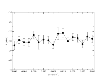
Figure 1: Results of a transient estimation for the ground state energy of a ⁸n started from an AFDMC calculation.

The errorbars are in any case rather large, which is due to a poor description of spin dependent correlations in both trial and guiding functions. They can be included by using the backflow form of ref.brualla03 . Work in this direction is in progress.

Another interesting comparison is with the results obtained with various energy density functional models, like (i) Skyrme Mkrivine80 , (ii) Skyrme 1’vautherin72 ; ravenhall72 , (iii) FPSpandharipande89 and (iv) FPS–21pethick95 , which reproduce the ground state energies of stable closed shell nuclei rather accurately. The energy density functional models provide a range of values for the binding energy of ${}^{8}n(0^{+})$ which goes from $-32.1$MeV of FPS to $-47.4$MeV of Skyrme Mpudliner96 . Moreover, the ${}^{7}n$ spin–orbit splitting is about $3$MeV, too large with respect to the quantum Monte Carlo estimates.

Table 2: Ground state AFDMC energies of ${}^{8}n(0^{+})$, ${}^{7}n(\frac{1}{2}^{-})$ and ${}^{7}n(\frac{3}{2}^{-})$ droplets for $V_{0}=20$MeV and the AU8’ and AU6’ interactions. The cluster variational Monte Carlo (CVMC) and GFMC results of ref.pieper01 for the AU8’ and the full AU18 (Argonne $v_{18}$ plus Urbana IX) are also reported for comparison. The last column reports the spin–orbit splittings (SOS) in MeV of ${}^{7}n$, given by the energy difference between the ${}^{7}n(\frac{3}{2}^{-})$ and ${}^{7}n(\frac{1}{2}^{-})$ states.

	${}^{8}n(0^{+})$	${}^{7}n(\frac{1}{2}^{-})$	${}^{7}n(\frac{3}{2}^{-})$	SOS
GFMC(AU18)	-37.8(1)	-33.2(1)	-31.7(1)	1.5(2)
CVMC(AU18)	-35.5(1)	-31.2(1)	-29.7(1)	1.5(2)
GFMC(AU8’)	-38.3(1)	-34.0(1)	-32.4(1)	1.6(2)
AFDMC(AU8’)	-37.8(2)	-32.5(2)	-31.8(1)	0.7(2)
AFDMC(AU6’)	-36.82(5)	-31.6(2)	-30.8(4)	0.8(5)

We have repeated the calculations of ground state energies and densities in the Skyrme 1’ and in the SKM models for the ${}^{8}n(0^{+})$ drop. The interaction parameters have been taken from Ref.pethick95 . The energies found are $-47.03$MeV and $-50.6$MeV respectively. In Fig. 2 we compare the neutron density profiles of the ${}^{8}n(0^{+})$ drop obtained from AFDMC calculations with $AU8^{\prime}$ and $AU6^{\prime}$ interactions, and from self consistent mean field calculations using the Skyrme 1’ model, and the SKM model.

As it can be seen, both of the energy density functional results differ significantly from the quantum Monte Carlo ones, particularly in the peak density value, at the center of the drop. The SKM however shows a density which is much closer to the quantum Monte Carlo result than the Skyrme 1’ one.

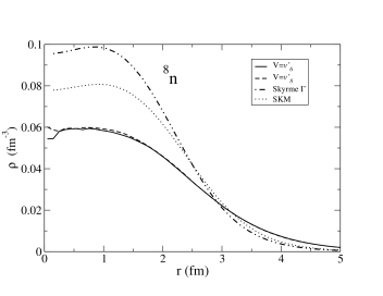
Figure 2: Density profiles for a ${}^{8}n$ drop for $V_{0}=20$MeV. Solid line: result with the $v^{8^{\prime}}$ interaction; dashed line: result with the $v^{6^{\prime}}$ interaction; dotted-dashed line: HF with Skyrme 1’; dotted line: SKM.

In Table 3 we report the results of AFDMC calculations for a ⁸n droplet for different values of the depth of the confining potential $V_{0}$. The importance function for each case was optimized only with respect to the parameters of the potential well from which the orbitals to be included in the Slater determinant are obtained.

Table 3: AFDMC ground state energy (in MeV) for a ⁸n droplet as a function of the parameter $V_{0}$ (in MeV) of $V_{ext}$. The energy difference $\Delta E=E(AU8^{\prime})-E(AU6^{\prime})$ gives an unbiased estimate of the spin–orbit interaction contribution.

$V_{0}$	$E_{T}$	$E_{AU8^{\prime}}$	$\langle V\rangle$	$\langle v_{\vec{L}\cdot\vec{S}}\rangle$	$E_{AU6^{\prime}}$	$\Delta E$
20	-26.27(7)	-37.8(2)	-124.6(3)	-0.41(7)	-36.82(5)	-1.0(2)
25	-48.0(3)	-60.5(1)	-168.2(4)	-0.59(4)	-59.6(1)	-0.9(2)
30	-69.3(3)	-85.3(2)	-201.3(2)	-0.72(4)	-83.7(1)	-1.6(4)
35	-92.7(3)	-111.0(2)	-232.4(2)	-0.71(3)	-109.86(5)	-1.1(4)

Together with the AFDMC energies we report the variational energies $E_{T}$. The difference between tha variational and the AFDMC energy is quite large, in all cases between 20 and 30%. This indicates that the evaluation of mixed estimators is at the same level of accuracy for all the cases, and the observed trends should not be too affected from the particular choice of the trial functions. The mixed energies are given for the $AU8^{\prime}$ and $AU6^{\prime}$ interactions, in order to calculate the contributions of the spin orbit interaction to the total energies. These are given in by $\Delta E$ on the last column of the figure.

We have also evaluated the mixed estimate of the spin–orbit interaction. Since $\langle\Psi|v_{\vec{L}\cdot\vec{S}}|\Psi\rangle=0$, the spin–orbit expectation value $\langle v_{\vec{L}\cdot\vec{S}}\rangle$ is approximately given by half the mixed estimate, and is reported in the fifth column of the Table. It is not very sensible to the depth of the potential well, in contrast with the total energy, which varies almost linearly with it.

One can see that $\langle v_{\vec{L}\cdot\vec{S}}\rangle$ is about 60% of $\Delta E$ in the range of depths of the well considered. On the other hand this value is very close to the spin–orbit splitting evaluated in the ${}^{7}n$ drop reported in Table II. It should also be noticed that in the latter case, the values of the spin–orbit splitting obtained with the AU8’ and the AU6’ are very similar. This means that the evaluation of the spin–orbit splitting in ${}^{7}n$ is not strongly influenced by the spin–orbit term in the interaction. The spin–orbit splitting found in our AFDMC is smaller (about one half) than the values reported from GFMC calculations. However, the consistencies in our results mentioned above makes us confident in the robustness of the evaluation of spin–orbit contributions in our method.

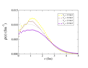
Figure 3: Neutron density profiles in a ${}^{8}n$ drop for different values of the depth of the confining potential $V_{0}$

In order to understand the connection between the parameter $V_{0}$ and the neutron density inside the drop, we have plotted in Fig. 3 the mixed estimators for the density profiles for all the confinements considered. Although the density at the center remains in a range $0.06<\rho(0)<0.09$fm^-3, it shows a larger dip at the center, and, consequently a stronger localization of neutrons at a distance of $\sim 1$fm, for larger values of $V_{0}$.

V Conclusions and perspectives

In this paper we have applied the Auxiliary Field Diffusion Monte Carlo method to the study of a closed-shell neutron drop ${}^{8}n(0^{+})$ and of the open shells ${}^{7}n(1/2^{-})$ and ${}^{7}n(3/2^{-})$ confined by an external Wood–Saxon field. The method compares rather well with standard GFMC techniques. Since the AFDMC, scales better than GFMC with the number of particles it is currently the only viable quantum Monte Carlo method to study large neutron rich systems.

We have made a detailed analysis of the contribution to the total energy of the spin-orbit interaction, which previous calculations on neutron mattersarsa03 has indicated as the main difference between AFDMC and GFMC calculations. Such analysis has been carried on at various values of the depth $V_{0}$ of the confining potential $V_{ext}$, and, therefore, for different confined neutron structures. We have found a spin-orbit contribution which is generally smaller than in GFMC calculations, confirming the findings of ref.sarsa03 . Such contribution lowers the binding energy of about 1 MeV in all considered cases.

The results obtained for the binding energies of the ${}^{7}n(1/2^{-})$ and ${}^{7}n(3/2^{-})$ droplets confirm earlier GFMC results on the spin orbit splittings, which are significantly smaller than those provided by the energy density functional models. The AFDMC value of the spin–orbit splitting is about one half of the value predicted by GFMC.

Future work includes improving the trial function $\Psi$, as well as the guiding function $\Psi_{G}$ for transient estimate. The properties of oxygen and flourine istopes can be calculated with the AFDMC method.

- (1) C. J. Pethick, D. G. Ravenhall, and C. P. Lorenz, Nucl. Phys. A 584, 675 (1982).
- (2) G. G. Raffelt, The stars as laboratories of fundamental physics (University of Chicago, Chicago & London, 1996).
- (3) K. L. Kratz, J. P. Bitouzet, F. K. Thielemann, P. Moeller, and B. Pfeiffer, Astrophys. J. 403, 216 (1993).
- (4) A. Akmal, V. R. Pandharipande, and D. G. Ravenhall, Phys. Rev. C 58, 1804 (1998).
- (5) J. M. Lattimer and M. Prakash, Astrophys. J. 550, 426 (2001).
- (6) R. F. Sawyer, Phys. Rev. D 11, 2740 (1975).
- (7) R. F. Sawyer, Phys. Rev. C 40, 865 (1989).
- (8) N. Iwamoto and C. J. Pethick, Phys. Rev. D 25, 313 (1982).
- (9) S. Reddy, M. Prakash, J. M. Lattimer, and J. A. Pons, Phys. Rev C 59, 2888 (1999).
- (10) S. Fantoni, A. Sarsa, and K. E. Schmidt, Phys. Rev. Lett. 87, 181101 (2001).
- (11) A. Smerzi, D. G. Ravenhall, and V. R. Pandharipande, Phys. Rev. C 56, 2549 (1997).
- (12) B. S. Pudliner, A. Smerzi, J. Carlson, V. R. Pandharipande, S. C. Pieper, and D. G. Ravenhall, Phys. Rev. Lett. 76, 2416 (1996).
- (13) S. C. Pieper, private communication (2003).
- (14) J. Carlson, J. Morales, Jr., V. R. Pandharipande, and D. G. Ravenhall (2003), eprint nucl-the/0303041.
- (15) A. Sarsa, S. Fantoni, K. E. Schmidt, and F. Pederiva (2003), eprint nucl-th/0303035.
- (16) K. E. Schmidt and S. Fantoni, Phys. Lett. B 446, 93 (1999).
- (17) S. C. Pieper, V. R. Pandharipande, R. B. Wiringa, and J. Carlson, Phys. Rev. C 64, 14001 (2001).
- (18) R. B. Wiringa, Argonne and Potential Package, http://www.phy.anl.gov/theory/research/ av18/av18pot.f (1994).
- (19) B. S. Pudliner, V. R. Pandharipande, J. Carlson, S. C. Pieper, and R. B. Wiringa, Phys. Rev C 56, 1720 (1997).
- (20) V. G. J. Stoks, R. A. M. Klomp, M. C. M. Rentmeester, and J. J. de Swart, Phys. Rev C 48, 792 (1993).
- (21) A. Akmal and V. R. Pandharipande, Phys. Rev. C 56, 2261 (1997).
- (22) M. Baldo and C. Maieron, Phys. Rev. C 69, 014301 (2004).
- (23) S. Fantoni and K. E. Schmidt, Nucl. Phys. A 690, 456 (2001).
- (24) R. B. Wiringa and S. C. Pieper, Phys. Rev. Lett. 89, 182501 (2003).
- (25) S. Fantoni, A. Sarsa, and K. E. Schmidt, Prog. Part. Nucl. Phys. 44, 63 (2000).
- (26) R. B. Wiringa, V. Fiks, and A. Fabrocini, Phys. Rev. C 38, 1010 (1988).
- (27) L. Brualla, S. A. Vitiello, A. Sarsa, S. Fantoni, and K. E. Schmidt, in preparation (2003).
- (28) H. Krivine, J. Treiner, and O. Bohigas, Nuc. Phys. A 336, 155 (1980).
- (29) D. Vautherin and D. M. Brink, Phys. Rev C 5, 626 (1972).
- (30) D. G. Ravenhall, C. D. Bennet, and C. J. Pethick, Phys. Rev. Lett. 28, 978 (1972).
- (31) V. R. Pandharipande and D. H. Ravenhall, in Proceedings of the NATO Advanced Research Workshop on Nuclear Matter and Heavy Ion Collisions, Les Houches. NATO-ASI, Ser. B, edited by M. S. et al. (Plenum, New York, 1989), vol. 205, p. 193.