The $\phi$ meson width in the medium from proton induced $\phi$ production in nuclei

Abstract

We perform calculations for the production of $\phi$ mesons in nuclei at energies just above threshold and study the $A$ dependence of the cross section. We use results for the $\phi$ selfenergy in the medium obtained within a chiral unitary approach. We find a strong $A$ dependence which is tied to the distortion of the incident proton and to the absorption of the $\phi$ in its way out of the nucleus. The effect of this latter process reduces the cross section in about a factor two in heavy nuclei proving that the $A$ dependence of the cross section bears valuable information on the $\phi$ width in the nuclear medium. Calculations are done for energies which are accessible in an experimental facility like COSY.

1 Introduction

The study of the properties of vector mesons in a nuclear medium is one of the subjects in hadron physics which receives continuous attention (see for instance Ref. [1]). Although originally the $\rho$ meson properties were mostly investigated, with the time the renormalization of the $\phi$ properties has been taking over as it is linked to the way kaons and antikaons are modified in the nuclear medium, which has also been the subject of intense study. One of the motivations for this latter work is the deviation of the $K^{-}$ selfenergy from the low density theorem, which is needed to reproduce kaonic atoms data [2, 3, 4, 5], together with the possibility of formation of kaon condensates in neutron stars [6].

Another reason why the $\phi$ properties have got a renewed interest is the fact that the medium renormalization in the case of the $\phi$ is relatively more drastic than that of the $\rho$. Indeed, predictions of an increase of the $\phi$ width by a factor five or six [7, 8] to ten [9], at normal nuclear matter density, have been made using different chiral approaches. This large width should in principle be detectable experimentally and, indeed, different reactions have been studied or suggested like $\phi$ production in $A-A$ collisions [10, 11], the reaction $\pi^{-}p\to\phi n$ in nuclei [9] or different methods based on inclusive $\phi$ photoproduction in nuclei [12, 13, 14].

The width of the $\phi$ has not been the only matter of concern and the possible shift of the mass has also captured attention. In that sense, the $\phi$ mass change has been studied in several approaches like using effective Lagrangians [9, 15, 16, 17, 18], QCD sum rules [19, 20] or the Nambu-Jona-Lasinio model [21]. In ultra-relativistic heavy ion collisions the $\phi$ width modification in matter has also been studied in a dropping meson mass scenario [17, 22, 23, 24, 25, 26], as a result of collisional broadening through $\phi$-baryon [27] or $\phi$-meson [28] scattering processes. All these works point at a sizeable renormalization of the $\phi$ width and a small mass shift. For this reason we will only be concerned about the $\phi$ width in the medium.

The aim of the present work is to propose a method to determine the $\phi$ width in the nuclear medium. The traditional method in the works quoted above (except [14]) is to look for a broadening of the $\phi$ width reconstructed from the invariant mass of its decay products. Here, instead, we use a different philosophy and we investigate the $A$ dependence of $\phi$ production in $pA$ collisions, in a similar way as it was done in [14] with the $\phi$ photoproduction in nuclei, which is the subject of experimental investigation at Spring8/Osaka [29]. The advantage of performing the reaction slightly above threshold is that one can rule out the contribution from coherent $\phi$ production which might obscure the interpretation of the experimental results in [29]. The present reaction, with its particular kinematics, is amenable of experimental performance at facilities like COSY.

2 Nuclear effects in the $\phi$ production

2.1 General formalism

In order to implement the relevant nuclear effects in the $\phi$ production cross section we will use a model based on many body techniques, successfully used in the past in many works [30, 31] to study the interaction of different particles with nuclei. The model assumes a local Fermi sea at each point in the nucleus and provides a very simple and accurate way to account for the Fermi motion of the initial nucleon and the Pauli blocking of the final ones. On the other hand, we have to take into account the distortion of the incoming nucleon and the final $\phi$ meson in the their way through the nucleus, which are evaluated in the present work using an eikonal approximation. In fact, the $A$ dependence of the effect due to the final $\phi$ absorption will provide the way to test the modification of the $\phi$ meson width in nuclear matter, as we will explain in much more detail in the following, and which is the main aim of the present work.

Within the local Fermi sea approach the nuclear cross section can be evaluated, as a first approximation, as:

$$\sigma_{A}(p_{Lab})=4\int d^{3}r\int\frac{d^{3}k}{(2\pi)^{3}}\Theta(k_{F}-|\vec{k}|)\sigma_{m}(p_{Lab},\vec{k},\vec{r})$$ (1)

since $4\int\frac{d^{3}k}{(2\pi)^{3}}\Theta(k_{F}-|\vec{k}|)=\rho(r)$, where $k$ is the momentum of the nucleon in the Fermi sea, $k_{F}$ the Fermi momentum at the local point, $\Theta$ the step function, $p_{Lab}$ the momentum of the incident proton and $\sigma_{m}$ the elementary $pp\to pp\phi$ and $pn\to pn\phi$ average cross section in the nuclear medium, which will be defined later in Eq. (8).

At this point we can add in Eq. (1) the following eikonal factor to account for the distortion of the incident proton in its way through the nucleus till the reaction point:

$$exp\left[-\int_{-\infty}^{z}\sigma_{pN}(p_{Lab})\rho(\sqrt{b^{2}+z^{\prime 2}})dz^{\prime}\right]$$ (2)

where $z$ and $\vec{b}$ are the position in the beam axis and the impact parameter, respectively, of the production point $\vec{r}$ of Eq. (1). In Eq. (2) $\sigma_{pN}$ is the total $pp$ and $pn$ averaged experimental cross section, taken from [32], for a given incident proton momentum. Eq. (2) represents the probability for the proton to reach the reaction point without having a collision with the nucleons, since $\sigma_{pN}\rho$ is the probability of proton collisions per unit length. The use of this eikonal factor will select the one-step processes and neglect the possibility that the $\phi$ is produced in a second collision of the nucleon, or a possible excited $\Delta$. We shall also take these two-step processes into account later on, but we advance that the $A$ dependence of the $\phi$ production cross section is already given quite accurately by the one-step process.

The final $\phi$ absorption in its way out of the nucleus can also be accounted for by means of a similar eikonal factor and for the evaluation of the probability of loss of flux per unit length we can proceed as follows: let $\Pi(p_{\phi},\rho(r))$ be the $\phi$ selfenergy in a nuclear medium as a function of its momentum, $p_{\phi}$, and the nuclear density, $\rho(r)$. We have

$$\frac{\Pi}{2\omega_{\phi}}\equiv V_{\textrm{opt}}=\ {\cal R}e{V_{\textrm{opt}}}\ +\ i\,{\cal I}m{V_{\textrm{opt}}}\ ,$$ (3)

and hence

$$\frac{\Gamma}{2}=-{\cal I}m\frac{\Pi}{2\omega_{\phi}}\quad;\qquad\Gamma=-\frac{{\cal I}m\Pi}{\omega_{\phi}}\equiv\frac{d{\cal P}}{dt}\ ,$$ (4)

where $\omega_{\phi}$ is the $\phi$ energy and ${\cal P}$ is the $\phi$ decay probability, including nuclear quasielastic and absorption channels. However, in what follows we shall only include in ${\cal I}m\Pi$ the absorption channels of the $\phi$, since in quasielastic $\phi$ collisions the nucleus will be excited but the $\phi$ will still be there to be observed. Hence, we have for the probability of loss of flux per unit length

$$\frac{d{\cal P}}{dl}=\frac{d{\cal P}}{v\,dt}=\frac{d{\cal P}}{\frac{p_{\phi}}{\omega_{\phi}}dt}=-\frac{{\cal I}m\Pi}{p_{\phi}}\ .$$ (5)

and the corresponding survival probability is given by

$$exp\left[-\int_{0}^{\infty}dl\frac{(-1)}{p_{\phi}}{\cal I}m\Pi(p_{\phi},\rho(r^{\prime}))\right],$$ (6)

where $\vec{r}\,^{\prime}=\vec{r}+l\frac{\vec{p}_{\phi}}{|\vec{p}_{\phi}|}$ with $\vec{r}$ the $\phi$ production point inside the nucleus. The study of the $A$ dependence of the total nuclear cross section due to the $\phi$ absorption effect, Eq. (6), is the main aim of this work, since it reflects the modification of the $\phi$ meson width in nuclear matter.

The study of the $A$ dependence was also done for $\eta$ photoproduction in [33], along the same lines as discussed above, in order to determine the inelastic $\eta N$ cross section in a nuclear medium. That paper also shows that an alternative BUU approach [34] gives similar results to the Glauber, or eikonal, approach.

Another relevant nuclear effect of sizeable consequences is the binding energy. When studying nuclear reactions with other beams, for instance photons, one usually neglects the binding energy, $V_{N}$, because it affects both the initial and outgoing nucleons and then it cancels in the $\delta$ function of energy conservation. Therefore, one usually considers only the kinetic energy of the nucleons. In the present reaction, with a proton as incident beam, the same cancellation happens, because we have two initial and two final nucleons. However, in order to neglect $V_{N}$ of the nucleons we must consider the kinetic energy of the nucleon beam at the reaction point which is bigger than the asymptotic value due to the attractive potential felt by the proton inside the nucleus. This increase in the kinetic energy can be evaluated considering that $E_{tot}=E_{kin}(asymptotic)=E_{kin}(local)+V_{s}(local)$, where $V_{s}$ is the potential due to the local Fermi sea, which in the Fermi model is $V_{s}(r)=-\epsilon_{F}(r)=\frac{-k_{F}^{2}(r)}{2M}$, with $k_{F}=(\frac{3}{2}\pi^{2}\rho(r))^{1/3}$ and $M$ the nucleon mass. With these considerations we can define the local initial proton momentum $\vec{p}\,^{\prime}_{Lab}$ such that

$$\sqrt{M^{2}+\vec{p}\,{{}^{\prime}}^{2}_{Lab}}=\sqrt{M^{2}+\vec{p}\,^{2}_{Lab}}+\frac{k_{F}^{2}(r)}{2M}.$$ (7)

This $p^{\prime}_{Lab}$ is the incident proton momentum used as input to evaluate the elementary cross section.

The elementary cross section in the nuclear medium for $p(p^{\prime}_{Lab})+N(k)\to N(p_{1})+p(p_{2})+\phi(p_{\phi})$ reaction is

$$\sigma_{m}(p^{\prime}_{Lab},\vec{k},\vec{r}) = \frac{M}{|\vec{p}_{Lab}|}\frac{1}{(2\pi)^{4}}\int d\Omega_{\phi}\int dp_{\phi}p^{2}_{\phi}\int{dp_{1}}\frac{p_{1}}{P}\frac{M^{2}}{2E(p_{1})\omega(p_{\phi})}\times$$ (8)

$$\times \overline{\sum_{s_{i}}}\sum_{s_{f}}|T|^{2}\Theta(p_{1}-k_{F}(r))\Theta(p_{2}-k_{F}(r))\Theta(1-A^{2})$$

where $P=p^{\prime}_{Lab}+k-p_{\phi}$, and $A$, providing the cosinus of the angle between $\vec{P}$ and $\vec{p}_{1}$, $A\equiv\frac{1}{2|\vec{P}||\vec{p}_{1}|}\left\{M^{2}+\vec{P}^{2}+\vec{p}\,^{2}_{1}-[E(p^{\prime}_{Lab})+E(k)-E(p_{1})-\omega(p_{\phi})]^{2}\right\}$, with $E(q)=\sqrt{M^{2}+\vec{q}\,^{2}}$, $\omega(q)=\sqrt{m_{\phi}^{2}+\vec{q}\,^{2}}$. In Eq. (8) the azimuthal angle of $\vec{p}_{1}$ with respect to $\vec{P}$ has already been integrated, assuming that $|T|^{2}$ does not depend on this angle. This is, however, supported by the experiment [35] where the angular dependence of $pp\to pp\phi$ is almost flat. Hence we assume in what follows $|T|^{2}$ to be angular independent.

Gathering all these results the final expression for the $\phi$ production cross section in nuclei reads:

$$\sigma_{A}(p_{Lab})=\frac{2}{(2\pi)^{7}}\frac{M^{3}}{|\vec{p}_{Lab}|}\int d^{2}b\int_{-\infty}^{\infty}dz\,exp\left[-\int_{-\infty}^{z}\sigma_{pN}(p_{Lab})\rho(\sqrt{b^{2}+z^{\prime 2}})dz^{\prime}\right]$$

$$\int d^{3}k\int{dp_{1}}\int d\Omega_{\phi}\int dp_{\phi}\frac{|\vec{p_{\phi}}|^{2}|\vec{p_{1}}|}{|\vec{P}|E(p_{1})\omega(p_{\phi})}\overline{\sum_{s_{i}}}\sum_{s_{f}}|T|^{2}\,exp\left[-\int_{0}^{\infty}dl\frac{(-1)}{|\vec{p_{\phi}}|}{\cal I}m\Pi(p_{\phi},\rho(r^{\prime}))\right]$$

$$\Theta(k_{F}-|\vec{k}|)\Theta(p_{1}-k_{F}(r))\Theta(p_{2}-k_{F}(r))\Theta(1-A^{2})\,.$$ (9)

As argued above, the $T$ matrix can be considered a constant for a given energy, which means that we can divide Eq. (9) by the free reaction cross section to get rid of $|T|^{2}$. The free reaction cross section can be easily evaluated as

$$\sigma_{free}(p_{Lab})=\frac{M^{3}}{|\vec{p}_{Lab}|}\frac{1}{(2\pi)^{3}}\int dE(p_{1})dE(p_{2})\Theta(1-B^{2})\Theta(\sqrt{s}-E(p_{1})-E(p_{2}))\overline{\sum_{s_{i}}}\sum_{s_{f}}|T|^{2}$$ (10)

where $B=(\sqrt{s}-E(p_{1})-E(p_{2}))^{2}-m_{\phi}^{2}-\vec{p_{1}}^{2}-\vec{p_{2}}^{2}/(2|\vec{p_{1}}||\vec{p_{2}}|)$.

The observable we will evaluate in the results section is $R\equiv\sigma_{A}/(A\sigma_{free})$ from Eqs. (9) and (10).

For the evaluation of ${\cal I}m\Pi$ in nuclear matter we use the results of the model of Ref. [8] and its extension to finite $\phi$-meson momentum done in [14]. This model is based on the modification of the $\bar{K}K$ decay channel in the medium by means of a careful treatment of the in medium antikaon selfenergies [7]. It uses a selfconsistent coupled channel unitary calculation, based on effective chiral Lagrangians, and taking into account Pauli blocking, pion selfenergies and mean-field potentials of the baryons (for the S-wave part) and hyperon-hole excitations (for the P-wave part).

In Fig. 1 we show the imaginary part of the $\phi$ selfenergy as a function of the $\phi$ momentum for different nuclear densities.

Figure 1: Imaginary part of the in medium $\phi$ selfenergy, without the inclusion of the free part, as a function of the momentum of the $\phi$ and the nuclear density. (From Ref. [14]). For a $\phi$ at rest and $\rho=\rho_{0}$ this corresponds to a $\phi$ in the medium width correction of $24\textrm{ MeV}$.

The contribution to $\Pi$ coming from the free $\phi$ decay into $K\bar{K}$, non density dependent, has been subtracted from the full $\Pi$ since the $K\bar{K}$ coming from the free decay would be detected and counted as a $\phi$ event, hence it does not contribute to the loss of flux required in the argument of the exponential in Eq. (6). As shown in [8], this corresponds to a $\phi$ medium width at rest at $\rho=\rho_{0}$ of the order of $24\textrm{ MeV}$.

At this point it is worth mentioning that we have used a local (momentum independent) nucleon selfenergy in Eq. (7). In practice it also has a momentum dependence which is often parametrized in terms of an effective mass [36]. We propose the following expression for the nucleon energy in the medium

$$E(p)=\sqrt{{M^{*}}^{2}+\vec{p}\,^{2}}+M-M^{*}-\frac{k_{F}^{2}}{2M^{*}}\,,$$ (11)

which at low momenta gives the nonrelativistic expression

$$E(p)=M+\frac{\vec{p}\,^{2}}{2M^{*}}-\frac{k_{F}^{2}}{2M^{*}}$$ (12)

used in many body approaches [36] with the Thomas Fermi energy as the local potential. Our expression (11), at the same time, provides a good relativistic energy of the nucleon in the low density limit. The effective mass $M^{*}$ is evaluated in accurate many body calculations [37, 38], which provide a $\rho$ dependence which can be approximated by

$$M^{*}=M\left(1-0.2\rho/\rho_{0}\right)\,.$$ (13)

At high energies, however, the use of Eq. (11) with the effective mass of Eq. (13) would overestimate the effect of nonlocalities, so our calculation using this approximation should be considered as an upper bound.

We have evaluated the $\phi$ production cross section modifying Eq. (7) to

$$\sqrt{{M^{*}}^{2}+\vec{p}\,{{}^{\prime}}^{2}_{Lab}}+M-M^{*}-\frac{k_{F}^{2}}{2M^{*}}=\sqrt{M^{2}+\vec{p}\,^{2}_{Lab}}\,,$$ (14)

and the expression for A (after Eq. (8)) by

$$A\equiv\frac{1}{2|\vec{P}||\vec{p}_{1}|}\left\{{M^{*}}^{2}+\vec{P}^{2}+\vec{p}\,^{2}_{1}-[E(p^{\prime}_{Lab})+E(k)-E(p_{1})-\omega(p_{\phi})]^{2}\right\}\,,$$ (15)

with $E(p)=\sqrt{{M^{*}}^{2}+\vec{p}\,^{2}}$. We shall comment in the results section that there are some small corrections coming from this source, but they do not modify the $A$ dependence of the results.

2.2 Two-step process with nucleon intermediate state

Now we want to improve the former result taking into account $\phi$ production from two-step processes. Let us imagine we have a $pN$ collision of the initial proton going to any other channel than $\phi$ production. In such cases the fast incoming proton will usually survive although with a reduced energy, by means of which it still can contribute to $\phi$ production. We estimate the contribution from this mechanism. The first step is to estimate the energy loss. The total $pN$ cross section for $T_{p}=2.5$ to $3$ GeV is around $40\textrm{ mb}$ and consist of $30$ % elastic and $70$ % inelastic, going mostly to several pion production. Estimating that the elastic collisions go in average around angles of $\theta=30^{o}$ or bigger in the CM frame since $\theta\in[0^{o},30^{o}]$ accounts for only $7$ % of the phase space, the $p$ energy loss in the lab frame is around $180\textrm{ MeV}$ or more. On the other hand, with an average three pions produced per collision, the amount of $500\textrm{ MeV}$ energy loss is a realistic figure. With the percentages given above for the elastic and inelastic collisions, one comes out with around $\Delta E\simeq 400\textrm{ MeV}$ loss per collision or more.

The probability that a $\phi$ is produced in a second step, after a prior $pN$ collision, is easily calculated assuming that the proton goes still forward after the $pN$ collision, which is essentially the case in the lab frame.

Since $\sigma_{pN}\rho(\vec{b},z^{\prime\prime})dz^{\prime\prime}$ is the probability of a $pN$ collision in $dz^{\prime\prime}$ then the formula to evaluate the cross section for this process is given by Eq. (9) substituting

$$\frac{1}{|\vec{p}_{Lab}|}\int_{-\infty}^{\infty}dz\,exp\left[-\int_{-\infty}^{z}\sigma_{pN}(p_{Lab})\rho(\sqrt{b^{2}+z^{\prime 2}})dz^{\prime}\right]F(p^{\prime}_{Lab})$$ (16)

$$\longrightarrow \frac{1}{|\vec{p}_{Lab}|}\int_{-\infty}^{\infty}dz^{\prime\prime}\int_{z^{\prime\prime}}^{\infty}dz\,exp\left[-\int_{-\infty}^{z^{\prime\prime}}\sigma_{pN}(p_{Lab})\rho(\sqrt{b^{2}+z^{\prime 2}})dz^{\prime}\right]\sigma_{pN}(p_{Lab})\rho(\sqrt{b^{2}+z^{\prime\prime 2}})$$

$$\qquad\qquad\qquad\qquad\quad\,\,\,\,exp\left[-\int_{z^{\prime\prime}}^{z}\sigma_{pN}(p_{Lab})\rho(\sqrt{b^{2}+z^{\prime 2}})dz^{\prime}\right]F(p^{\prime\prime}_{Lab})$$

where we have introduced a new integration over $z^{\prime\prime}$, the point of primary $pN$ collision and the two exponential factors account for the probability that the proton reaches the point $z^{\prime\prime}$ without any collision, times the probability that the struck proton reaches the $\phi$ production point without any other collision. In this sense we guarantee that there is one and only one primary $pN$ collision. In Eq. (16) the function $F$ corresponds to the rest of the integral and factors in Eq. (9) as a function of the proton momentum in the nucleus. Hence, $p^{\prime\prime}_{Lab}$, which will be the proton momentum after the primary collision is given by

$$\sqrt{\vec{p}\,{{}^{\prime\prime}}^{2}_{Lab}+M^{2}}=\sqrt{\vec{p}\,{{}^{\prime}}^{2}_{Lab}+M^{2}}-\Delta E.$$ (17)

2.3 Two-step processes with $\Delta$ intermediate states

In production processes below or close to threshold, multistep processes are usually important as we have already mentioned. Also it is known that $\Delta$ production in intermediate states is sometimes an efficient way to produce the final particles. Two methods among many, have particularly been used with success to deal with these multistep processes, and not necessarily around threshold, but particularly above it where some of the simplifications done are more accurate. One of the methods used is the transport equations [39, 34, 40] (BUU) in which there are collisions of the incoming particles which produce certain final states. In particular, $\Delta$ states are formed and allowed to propagate till they collide with other nucleons. These $\Delta$’s are assumed to be elementary particles, although the finite lifetime is taken into account. Another method which has been used in a large variety of physical problems is a computer simulation of the reactions [30, 41, 42, 43], with similarities to the cascade models. This method, originally developed to deal with pionic reactions [30], has also been used to deal with pion [41] and nucleon emission [42] in photonuclear reactions and in nucleon emission in electron nucleus scattering [43]. There is an essential difference between the transport method and the computer simulation of [30, 41, 42, 43]. In the latter one a quantum mechanical many body treatment of the process is done in which the $\Delta$’s are never elementary particles, but they appear as propagators in Feynman many body diagrams, which would qualify as two or three body processes in the transport method. The difference is more than technical since this procedure allows one to sum over the spin of the $\Delta$’s in amplitudes (in the propagator) while in the transport method the sums over spins are done on the cross sections. This leads sometimes to differences in angular distributions, the information of which might be missed in the transport method. However, sometimes, corrections are done in the standard BUU equations to account for these missing angular correlations [44]. The Monte Carlo simulation of [30, 41, 42, 43] evaluates quantum mechanically these multistep processes for the diagrams which are called irreducible. In this context reducible diagrams are those that, by cutting a propagator line of a stable particle in the diagram of an amplitude, two valid diagrams result, which can be interpreted as a multistep process with stable particles in the intermediate states. These processes can be reduced to a sequence of the more elementary ones. Their probabilities are calculated with the rules for irreducible diagrams, and the multistep ramification is done using a Monte Carlo simulation procedure, allowing the individual steps to occur according to the calculated probability.

Let us address now with the many body techniques, using irreducible Feynman diagrams, the analogous of the two-step process $NN\rightarrow N\Delta$ followed by $\Delta N\rightarrow NN\phi$ in the transport equation.

This two body process would benefit with respect to the one considered in the former subsection from the fact that the $\Delta$ couples more strongly to pions and vectors than the nucleon. For instance, one can consider a mechanism from the model of [45, 46] like the one on Fig. 2, which, with respect to the same one with a nucleon instead of a $\Delta$, would benefit from the factor $f_{\pi N\Delta}/f_{\pi NN}=f_{\rho N\Delta}/f_{\rho NN}=2.13$ in the amplitude, hence a factor 4.5 in the cross section.

Figure 2: Example of one of the possible diagrams for the $\Delta N\rightarrow NN\phi$ reaction [45, 46].

We shall distinguish between $\Delta$ excitation on the target and $\Delta$ excitation on the projectile. These two mechanisms appear in the elementary reaction $pp\to\Delta N$ [47, 48, 49], but they proved to be relevant in the $(^{3}\textrm{He},t)$ reaction in nuclei [50] and in the $(\alpha,\alpha^{\prime})$ reaction. In this latter case, only $\Delta$ excitation in the projectile is allowed [51], which was clearly seen experimentally in [52]. We describe below the two mechanisms starting from the $\Delta$ excitation on the target.

We now take the diagram shown in Fig. 3 b), which can be interpreted as having a $NN\rightarrow N\Delta$ collision followed by $\Delta N\rightarrow NN\phi$. No specific model is assumed for $\Delta N\rightarrow NN\phi$, which is indicated in Fig. 3 b) with the serrated line, as we neither did for the $NN\rightarrow NN\phi$, but, based on the arguments given above, we will simple assume that this process has a cross section about $4.5$ times bigger than $NN\rightarrow NN\phi$.

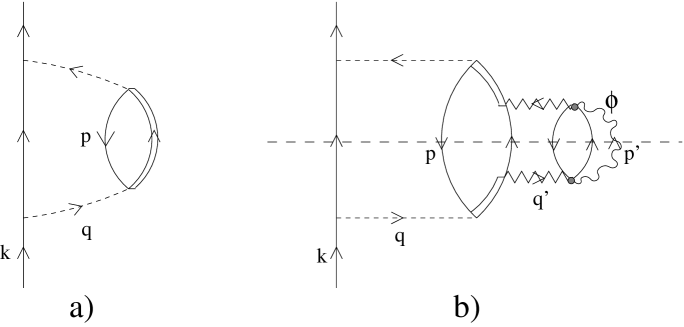
Figure 3: Diagram for the $NN\rightarrow N\Delta$ reaction for $\Delta$ excitation on the target a). Previous mechanism followed by the $\Delta N\rightarrow NN\phi$ process b). The long-dashed line represents the cut for the calculation of the imaginary part of the selfenergy.

We evaluate the contribution of the diagram of Fig. 3 b) to the nucleon selfenergy in the medium. A similar diagrammatic approach was used in [46] to account for corrections to ordinary multistep processes but including only nucleons in the intermediate states. However, it was rightly concluded there that the equivalent mechanisms with $\Delta$ intermediate states should be more important than the mechanisms evaluated there.

We calculate diagram 3 b) in two steps. First we evaluate the selfenergy of the incident proton due to the generic diagram of Fig. 3 a):

$$-i\Sigma(k)=3\int\frac{d^{4}q}{(2\pi)^{4}}\left(\frac{f_{\pi NN}}{m_{\pi}}\right)^{2}\vec{\sigma}\cdot\vec{q}\ \vec{\sigma}\cdot(-\vec{q})\ \frac{i}{{q^{0}}^{2}-\vec{q}\,^{2}-m_{\pi}^{2}-\Pi_{\Delta}}\ \frac{M}{E_{N}(\vec{k}-\vec{q})}\times$$

$$\times\left[\frac{i(1-n(\vec{k}-\vec{q}))}{k^{0}-q^{0}-E_{N}(\vec{k}-\vec{q})+i\epsilon}+\frac{in(\vec{k}-\vec{q})}{k^{0}-q^{0}-E_{N}(\vec{k}-\vec{q})-i\epsilon}\right]\,,$$ (18)

where the factor $3$ is an isospin factor and $\Pi_{\Delta}$ represents the pion selfenergy for $\Delta h$ excitation. One can now perform a Wick rotation as it is done in [53], see Fig. 4. The integral along the imaginary axis only contributes to the real part of $\Sigma$, and using the contour in the complex plane of the variable $q^{0}$ shown in the figure, one picks up only the nucleon pole of the $1-n(\vec{k}-\vec{q})$ term in Eq. (18), hence $q^{0}$ becomes $k^{0}-E_{N}(\vec{k}-\vec{q})$. One then obtains the imaginary part of the selfenergy, corresponding to the cut shown in Fig. 3 b), as

$${\cal I}m\Sigma(k)=3\left(\frac{f_{\pi NN}}{m_{\pi}}\right)^{2}\int\frac{d^{3}q}{(2\pi)^{3}}(1-n(\vec{k}-\vec{q})){\vec{q}\,}^{2}\frac{{\cal I}m\Pi_{\Delta}}{\left|(k^{0}-E_{N}(\vec{k}-\vec{q}))^{2}-\vec{q}^{2}-m_{\pi}^{2}-\Pi_{\Delta}\right|^{2}}\,,$$ (19)

where ${\cal I}m\Pi_{\Delta}$ accounts for all possible decay channels of the $\Delta$ (like $N\pi$ or $Nph$ or $Nph\phi$).

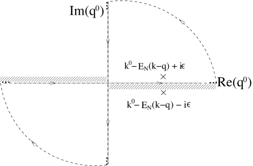
Figure 4: Analytic structure and contour used in the $q^{0}$ integral of Eq. (18) (Wick rotation). The shadowed regions represent the position of the cuts from the renormalized pion propagator.

The mechanism of $\phi$ production will pick up from ${\cal I}m\Pi_{\Delta}$ in the numerator of Eq. (19) only the process with $\phi$ production, but in the denominator ${\cal I}m\Pi_{\Delta}$ will appear accounting for all the $\Delta$ decay channels, out of which only the most relevant, $N\pi$, will be kept.

$\Pi_{\Delta}$ can be calculated in the same way and a final expression can be found in the appendix of [54]. For our purpose it is sufficient to take

$$\Pi_{\Delta}(q)=\frac{4}{9}\left(\frac{f_{\pi N\Delta}}{m_{\pi}}\right)^{2}{\vec{q}\,}^{2}\rho\,\frac{1}{\sqrt{s_{\Delta}}-M_{\Delta}-\frac{M_{\Delta}}{E_{\Delta}(\vec{q})}\Sigma_{\Delta}}\,\frac{M_{\Delta}}{E_{\Delta}(\vec{q})}\,,$$ (20)

where $\rho$ is the nuclear density and $s_{\Delta}=(q^{0}+M)^{2}-{\vec{q}\,}^{2}$. In Eq. (20) and in what follows we have neglected the three-momentum, $\vec{p}$, of the nucleons in the Fermi sea in the energy denominator since these momenta are small compared to typical values of $q$ and $k$. Note that we are keeping the $M_{\Delta}/E_{\Delta}(\vec{q})$ relativistic factors. ¿From Eq. (20) we find

$${\cal I}m\Pi_{\Delta}(q)=\frac{4}{9}\left(\frac{f_{\pi N\Delta}}{m_{\pi}}\right)^{2}{\vec{q}\,}^{2}\rho\left(\frac{M_{\Delta}}{E_{\Delta}(\vec{q})}\right)^{2}\frac{{\cal I}m\Sigma_{\Delta}}{\left|\sqrt{s_{\Delta}}-M_{\Delta}-\frac{M_{\Delta}}{E_{\Delta}(\vec{q})}\Sigma_{\Delta}\right|^{2}}\,.$$ (21)

For $\Pi_{\Delta}$ in the denominator of Eq. (19) it is sufficient to use Eq. (20) putting $\Sigma_{\Delta}=-i\Gamma(s_{\Delta})/2$, where $\Gamma(s_{\Delta})$ is the $\Delta$ width for $\pi N$ decay. However, in the numerator of Eq. (19), ${\cal I}m\Pi_{\Delta}$ is given by Eq. (21) where ${\cal I}m\Sigma_{\Delta}$ in the numerator should only account for $\phi$ production. In this way, when ${\cal I}m\Pi_{\Delta}$ is placed in the numerator of Eq. (19) it leads to the relevant term of $\phi$ production shown in Fig. 3 b). Thus, we need to evaluate the $\Delta$ selfenergy for the process shown in Fig. 5.

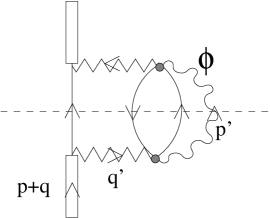
Figure 5: $\Delta$ selfenergy diagram accounting for the $\Delta N\rightarrow NN\phi$. The long-dashed line represents the cut for the calculation of the imaginary part of the selfenergy.

This diagram can be easily evaluated and gives (neglecting in the $\Delta$ four-momentum, $p+q$, the momentum $\vec{p}$ of the nucleon in the Fermi sea):

$$-i\Sigma_{\Delta}(p+q)=\int\frac{d^{4}q^{\prime}}{(2\pi)^{4}}\int\frac{d^{4}p^{\prime}}{(2\pi)^{4}}(-iT)(-iT)iU(q^{\prime}-p^{\prime})\times$$

$$\times\frac{M}{E_{N}(\vec{q}-\vec{q^{\prime}})}\ \frac{i(1-n(\vec{q}-\vec{q^{\prime}}))}{p^{0}+q^{0}-q^{\prime 0}-E_{N}(\vec{q}-\vec{q^{\prime}})+i\epsilon}\ \frac{i}{{p^{\prime 0}}^{2}-{\vec{p^{\prime}}\,}^{2}-m_{\phi}^{2}+i\epsilon}\,,$$ (22)

where $U(q^{\prime}-p^{\prime})$ is the Lindhard function [55] with the normalization of the appendix of [54], and we have only kept the particle part of the nucleon propagator (the only one which contributes to the imaginary part, as we saw when doing the Wick rotation). In Eq. (22) $T$ is the $\Delta N\rightarrow NN\phi$ amplitude, which we simple assume to be $2.13$ times bigger than the $NN\rightarrow NN\phi$ one.

Then ${\cal I}m\Sigma_{\Delta}$ can now be obtained again using a Wick rotation, or easier, applying Cutkosky rules [56] adjusted for the present problem [57] for the cut shown in Fig. 5:

$$\Sigma_{\Delta}\rightarrow 2i{\cal I}m\Sigma_{\Delta}\,,$$

$$U(q^{\prime}-p^{\prime})\rightarrow 2i\Theta(q^{\prime 0}-p^{\prime 0}){\cal I}mU(q^{\prime}-p^{\prime})\,,$$

$$G(p+q-q^{\prime})\rightarrow 2i\Theta(q^{0}+p^{0}-q^{\prime 0}){\cal I}mG(p+q-q^{\prime})\,,$$

$$D(p^{\prime})\rightarrow 2i\Theta(p^{\prime 0}){\cal I}mD(p^{\prime})\,,$$

where $G$ and $D$ are correspondingly nucleon and $\phi$ propagators. These rules lead to the expression

$${\cal I}m\Sigma_{\Delta}(k)=\int\frac{d^{3}q^{\prime}}{(2\pi)^{3}}\int\frac{d^{3}p^{\prime}}{(2\pi)^{3}}[1-n(\vec{q}-\vec{q^{\prime}})][1-n(\vec{q^{\prime}}-\vec{p^{\prime}})]|T|^{2}\times$$

$$\times\frac{1}{2\omega_{\phi}(p^{\prime})}(-\pi)\,\rho\,\delta(k^{0}+2M-E_{N}(\vec{k}-\vec{q})-E_{N}(\vec{q}-\vec{q^{\prime}})-E_{N}(\vec{q^{\prime}}-\vec{p^{\prime}})-\omega_{\phi}(p^{\prime}))\,,$$ (23)

which shows explicitly the $\delta$-function of energy conservation for the process $NNN\rightarrow NNN\phi$. In Eq. (23) we have used the following approximation:

$${\cal I}mU(q^{\prime}-p^{\prime})\simeq-\pi\rho[1-n(\vec{q}-\vec{q^{\prime}})]\delta(q^{\prime 0}-p^{\prime 0}+M-E_{N}(\vec{q^{\prime}}-\vec{p^{\prime}}))$$ (24)

Altogether we obtain the following expression for ${\cal I}m\Sigma(k)$ in Eq. (19):

$${\cal I}m\Sigma(k)=-\frac{1}{4\pi}\frac{4}{3}\left(\frac{f_{\pi N\Delta}}{m_{\pi}}\right)^{2}\left(\frac{f_{\pi NN}}{m_{\pi}}\right)^{2}\rho^{2}|T|^{2}\int\frac{d^{3}q}{(2\pi)^{3}}\int\frac{d^{3}q^{\prime}}{(2\pi)^{3}}\int dp^{\prime}\times$$

$$\times\frac{|\vec{p^{\prime}}|}{|\vec{q^{\prime}}|}\frac{M}{E_{N}(\vec{k}-\vec{q})}\frac{M}{E_{N}(\vec{q}-\vec{q^{\prime}})}M{\vec{q}\,}^{4}\frac{1}{2\omega_{\phi}(p^{\prime})}[1-n(\vec{k}-\vec{q})][1-n(\vec{q^{\prime}}-\vec{p^{\prime}})][1-n(\vec{q}-\vec{q^{\prime}})]\left(\frac{M_{\Delta}}{E_{\Delta}(\vec{q})}\right)^{2}\times$$

$$\times\left|\frac{1}{(k^{0}-E_{N}(\vec{k}-\vec{q}))^{2}-\vec{q}^{2}-m_{\pi}^{2}-\Pi_{\Delta}(q)}\right|^{2}\left|\frac{1}{\sqrt{s_{\Delta}}-M_{\Delta}-\frac{M_{\Delta}}{E_{\Delta}(\vec{q})}\Sigma_{\Delta}}\right|^{2}F(q)^{4}\times$$

$$\times\Theta(1-\cos(\theta_{\vec{p^{\prime}}\vec{q^{\prime}}})^{2})\,\Theta(k^{0}+2M-E_{N}(\vec{k}-\vec{q})-E_{N}(\vec{q}-\vec{q^{\prime}})-\omega_{\phi}(p^{\prime})-M)\,,$$ (25)

with

$$\cos(\theta_{\vec{p^{\prime}}\vec{q^{\prime}}})=\frac{1}{2|\vec{p}^{\prime}||\vec{q}^{\prime}|}\left\{M^{2}+\vec{p^{\prime}}\,^{2}+\vec{q^{\prime}}\,^{2}-[k^{0}+2M-E_{N}(\vec{k}-\vec{q})-E_{N}(\vec{q}-\vec{q^{\prime}})-\omega_{\phi}(p^{\prime})]^{2}\right\}\,.$$

In Eq. (25) we have already explicitly introduced a form factor $F(q)$ for any $\pi NN$ and $\pi N\Delta$ vertices

$$F(q)=\frac{\Lambda^{2}-m_{\pi}^{2}}{\Lambda^{2}-q^{2}}$$

with $\Lambda=1\ \textrm{ GeV}$, as usually done.

Next we want to interpret ${\cal I}m\Sigma(k)$ in terms of a cross section for $\phi$ production. We follow [58, 57] and write:

$$\Gamma=-2\frac{M}{E_{N}(k)}{\cal I}m\Sigma(k)$$ (26)

for the probability of $\phi$ production per unit time, keeping the important relativistic factors. Then

$$\frac{d{\cal P}}{dl}=-2M\frac{{\cal I}m\Sigma(k)}{|\vec{k}|}$$ (27)

and the cross section for the process, taking into account the initial proton distortion and the final $\phi$ distortion, is given by

$$\sigma=\int d^{3}r\,\,exp\left[-\int_{-\infty}^{z}\sigma_{pN}(p_{Lab})\right]\left[-2M\frac{{\cal I}m\widetilde{\Sigma}(p_{lab})}{|\vec{p}_{lab}|}\right]\,,$$ (28)

where ${\cal I}m\widetilde{\Sigma}(p_{lab})$ is calculated with the same expression as in Eq. (25) including in addition the final $\phi$ distortion factor of Eq. (6),

$$exp\left[-\int_{0}^{\infty}dl\frac{(-1)}{|\vec{p}_{\phi}|}{\cal I}m\Pi(p_{\phi},\rho(r^{\prime}))\right].$$ (29)

We simplify the calculations by assuming the $\phi$ to go in the forward direction, $\vec{p}_{\phi}=(0,0,p^{\prime})$, which is a good approximation in the nucleus rest frame, where the calculations are done, as we have checked.

Next we briefly describe how to take into account $\Delta$ excitation in the projectile taking advantage of the formalism described above. The relevant diagram that we should consider is given in Fig. 6.

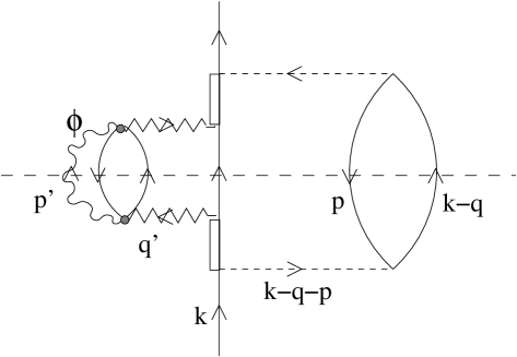
Figure 6: Diagram for the two-step $\phi$ production with intermediate $\Delta$ excited on the projectile.

The notation for the momenta in Fig. 6 have been chosen to keep maximum analogy with the previous mechanism. Hence the same formulae as before can be used adding to ${\cal I}m\Sigma(k)$ of Eq. (25) for $\Delta$ excitation in the target another term ${\cal I}m\Sigma^{\prime}(k)$ to account for $\Delta$ excitation on the projectile, which has the same expression as Eq. (25) with the following changes:

$${\vec{q}\,}^{4}\to(\vec{k}-\vec{q})^{4},$$

$$F(q)\to F(k-q-p),$$

$$\frac{1}{(k^{0}-E_{N}(\vec{k}-\vec{q}))^{2}-\vec{q}^{2}-m_{\pi}^{2}-\Pi_{\Delta}(q)}$$

$$\to\frac{1}{(E_{N}(\vec{k}-\vec{q})-M)^{2}-(\vec{k}-\vec{q})^{2}-m_{\pi}^{2}-\Pi_{\Delta}(k-q-p)}.$$ (30)

Let us note that the last mechanism is similar to the two-step mechanism with only nucleons studied above in subsection 2.2. In the latter case, the projectile nucleon loses some energy and later on collides with other nucleons to produce the $\phi$. In the mechanism of Fig. 6 the projectile gets excited to a $\Delta$ and this $\Delta$ collides with other nucleons to produce the $\phi$. Since we estimated the cross section for $\Delta N\to NN\phi$ to be about four times bigger than for $NN\to NN\phi$, we should expect that the mechanism of Fig. 6 should be more relevant than the two-step mechanism involving only nucleons. This is indeed the case, as we shall see in the results, showing also that the mechanism of $\Delta$ excitation in the projectile is more important than that of $\Delta$ excitation in the target in the present reaction.

It is worth mentioning that this diagrammatic method cannot be directly used for the two-step nucleon mechanism, because if a nucleon replaces the $\Delta$ in the diagram of Fig. 6 this nucleon could be on-shell and would live forever, thus producing formally an infinite amount of $\phi$ in its collision with infinite nuclear matter, where the calculations are done. This is not the case for the $\Delta$ due to the short lifetime. Hence, in this case the infinite matter approach, together with the local density approximation (also used in the calculations), can be reliably used. For the nucleon case the explicit consideration of the finite size of the nucleus is essential. This is the reason for the different treatment of these two processes in spite of their similarity. These arguments are further elaborated in [59].

3 Results and discussion

Figure 7: The results of our calculations for proton kinetic energy $T_{p}=2.7\textrm{ GeV}$ with only one-step process. Different lines correspond to separate contributions from the PS, ISI, FSI and total cross section.

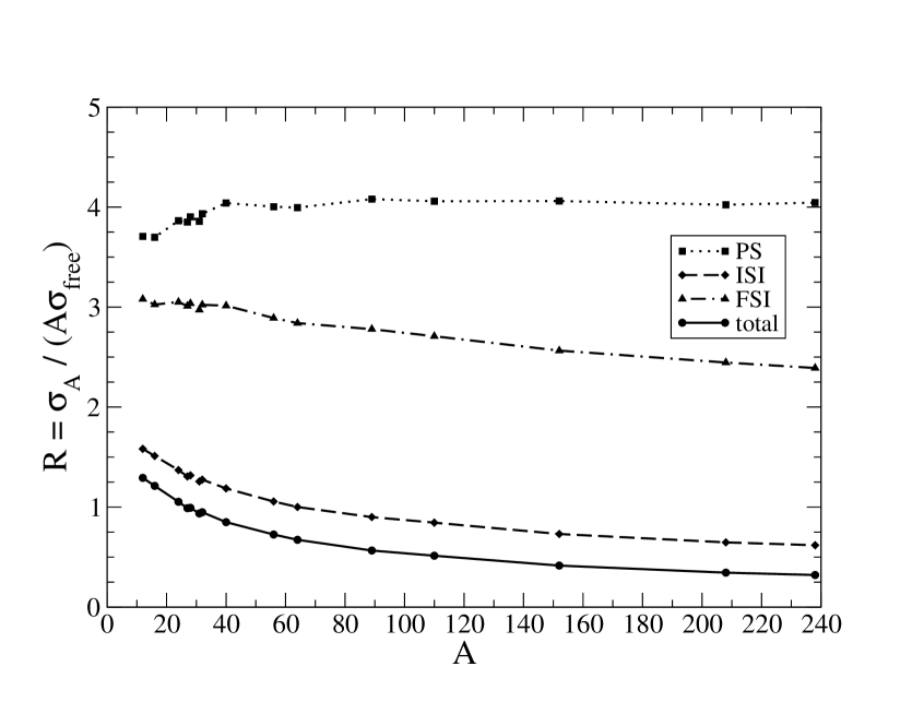
Figure 8: The same as Fig. 7, but for proton kinetic energy energy $T_{p}=2.83\textrm{ GeV}$.

First we want to present results from the model of subsection 2.1, accounting for the one-step process. In Figs. 7 and 8 we show the results for $R=\sigma_{A}/(A\sigma_{free})$ for the projectile energies $T_{p}=2.7$ and $2.83\textrm{ GeV}$ respectively. Different lines correspond to separate contributions from the phase space (PS), Eq. (1); phase space and initial state interaction, Eq. (1) including the distortion factor of Eq. (2), (ISI); phase space and final state interaction, Eq. (1) including the distortion factor of Eq. (6), (FSI); and complete calculation, (total), i.e. the simultaneous contribution of all the effects, Eq. (9). We performed calculations for the following nuclei: ${}^{12}_{6}C$, ${}^{16}_{8}O$, ${}^{24}_{12}Mg$, ${}^{27}_{13}Al$, ${}^{28}_{14}Si$, ${}^{31}_{15}P$, ${}^{32}_{16}S$, ${}^{40}_{20}Ca$, ${}^{56}_{26}Fe$, ${}^{64}_{29}Cu$, ${}^{89}_{39}Y$, ${}^{110}_{48}Cd$, ${}^{152}_{62}Sm$, ${}^{208}_{82}Pb$, ${}^{238}_{92}U$.

By looking at the PS curves of Figs. 7 and 8, we see that $R$ is larger than unity in both cases and much larger for the lower $T_{p}$. This is due to the Fermi motion. This increase of the nuclear cross section over $A\sigma_{free}$ is a well known fact in subthreshold production in particle-nucleus as well as in nucleus-nucleus collisions [60, 61]. The reaction threshold is defined for the scattering on a nucleon at rest. Yet, at this threshold energy, the Fermi motion of the nucleons makes the reaction possible and the ratio $R$ would grow up to infinity as we approach the threshold energy. At subthreshold energies, the consideration of large momentum components of the nucleons in the nucleus by means of the spectral function, accounting simultaneously for important correlations between energy and momentum [38, 62], helps to increase the cross section [63], as well as the consideration of multi scattering processes [64, 65]. All these mechanisms become progressively less and less important as we go up to energies above threshold, and as we discuss below, the possible uncertainty of our results from neglecting these sources will not modify our conclusions, since we are interested in the form of the $A$-dependence of the cross section rather than in its absolute value. Indeed, the PS curve is practically constant with a good accuracy for all $A$. The effects discussed above, from the spectral function and multinucleon scattering mechanisms, are volume effects, not affected by the distortion of the initial proton or the absorption of the final $\phi$. Thus the constancy in $A$ of the corresponding PS calculations including these new effects would also hold with a somewhat increased cross section. Now if we look at ISI and FSI curves, we see that in both cases there is a sizeable decrease of $R$, particularly for ISI, which shows a stronger $A$ dependence. Although the ISI and ”total” curves are almost parallel, the absolute values decrease with $A$ and therefore the contribution of the FSI becomes more and more important. This significant $A$ dependence can be seen in the ratio of these two curves which is shown in Fig. 9.

Figure 9: Ratio of the total cross section to ISI with only one-step process. Calculations are done for $T_{p}=2.83\textrm{ GeV}$.

We see that the ratio decreases from values around $0.8$ for light nuclei to values close to $0.5$ for heavy nuclei. From this figure we can conclude that in the $A$-dependence there is indeed valuable information concerning the $\phi$ absorption and hence, the $\phi$ width in the medium, which is the main conclusion of the present work.

At this point we want to discuss the effect of taking into account the momentum dependence of the nucleon selfenergy. By doing the changes explained in Eqs. (14) and (15) we find an increase of about 15% in the cross sections (which we would consider as an upper bound), but this percentage increase is remarkably equal for all nuclei such that the A dependence of the curves in Figs. 7, 8 is preserved. This means that if we normalize the cross section to the one of the given nucleus, as we shall do later, the effect discussed above does not show up.

Now we pass to consider the contribution from the two-step processes with nucleon and $\Delta$ intermediate states. In Figs. 10 and 11 we plot the ratios of the different two-step mechanisms to the one-step process for two different energies as a function of the mass number.

Figure 10: Ratio of the nuclear cross section of the different two-step processes over the cross section of the one-step process. The different lines represent: dotted line, only nucleons as intermediate state with $\Delta E=300\textrm{ MeV}$ (see subsection 2.2); dashed-dotted line, only nucleon with $\Delta E=400\textrm{ MeV}$; solid line, intermediate $\Delta$ excited on the target (see Fig. 5); dashed line, intermediate $\Delta$ excited on the projectile (see Fig. 6). The calculations are done for a kinetic energy of the beam proton of $T_{p}=2.7\textrm{ GeV}$.

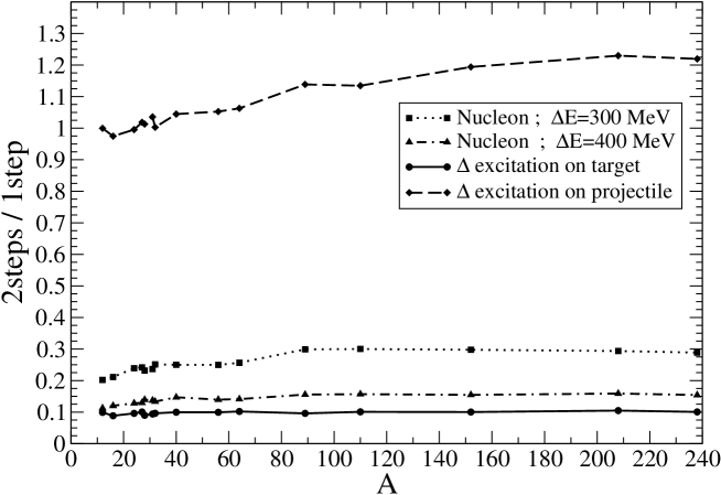
Figure 11: Same as Fig. 10 but for $T_{p}=2.83\textrm{ GeV}$.

We see that the most important two-step contribution comes from the $\Delta$ excitation in the projectile which is comparable to the one-step mechanism and about $5-10$ times bigger than the two-step mechanism involving only nucleons or $\Delta$ excitation on the target. Even then, we are concerned about the $A$ dependence, no so much on the absolute values of the cross sections, since the $\phi$ absorption effect is reflected in this $A$ dependence.

The relevance of the two step processes in $\phi$ production was also put of manifest in Ref. [66]. There it was shown that the two step mechanism, in which a pion is produced in the intermediate states was dominant below threshold, but small compared to the one step process at the energies studied here. We estimate our two step cross section involving $\Delta$ in the intermediate states to be of the same order as the one step process. We should note, however, that the two step processes involving $\pi$ or $\Delta$ in the intermediate are not the same, in the sense that the serrated line in Figs. 3 and 6 does not necessary stand for an on shell pion. Actually, as shown in [46], having in this line intermediate $\rho$ states leads to a much larger two step contribution. We accept uncertanties from the two step mechanism, but then we look for one observable that minimizes these uncertanties and this is given by the $A$ dependence of the cross section. Indeed, the fact that the curves in Figs. 10 and 11 are almost flat as a function of $A$ indicates that the $A$ dependence of the sum of all mechanisms has essentially the same $A$ dependence as the one-step mechanism alone. To see this more clearly, we show in Fig. 12 the ratio $R(^{A}X)$ normalized to $R(^{12}C)$ for the one-step and one- plus two-step mechanisms.

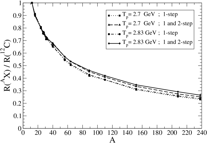
Figure 12: Ratio of the nuclear cross section normalized to ${}^{12}C$ for two different incident proton kinetic energies, $T_{p}$, including or not the two-step mechanisms. The two-step process with nucleon intermediate states has been evaluated with $\Delta E=400\textrm{ MeV}$.

What we see in the figure is that this normalized $R$ changes very little when including the two-step mechanisms for both the $T_{p}$ considered. Note that for the energy closer to the threshold ($T_{p}=2.7\textrm{ GeV}$) the changes due to the two-step contributions are smaller. Therefore we conclude that the $A$ dependence obtained in the present work is reliable and the calculations clearly show that proton induced $\phi$ production in nuclei at energies just above threshold can indeed be used to get information on the $\phi$ width in the medium.

In order to see which is the experimental precision needed to get a definite information on the $\phi$ width in the medium, we have performed the same calculations assuming $\phi$ widths in the medium to be one half or twice the width used so far [8, 14]. In the calculations this is implemented by multiplying the argument of the exponential in Eq. (6) by $1/2$ or $2$ respectively. In Fig. 13 we show the results of these calculations for $T_{p}=2.83\textrm{ MeV}$ (without the inclusion of the two-step processes).

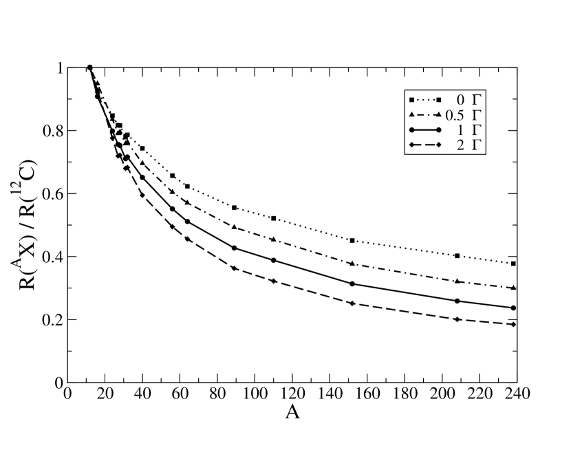
Figure 13: Ratio of the nuclear cross section normalized to ${}^{12}C$ for $T_{p}=2.83\textrm{ GeV}$ multiplying the $\phi$ width in the medium by different factors.

Comparing Figs. 12 and 13 we clearly see that the uncertainties due to the second step mechanism are far smaller than the differences in the results obtained by using these different $\phi$ widths. The three curves shown there for the width of [8, 14], half this width, and double, should serve to get a fair answer about the $\phi$ width in the medium by comparing with experimental results. Comparing Figs. 12 and 13 one can see that the uncertainties one might have from the approximate knowledge of the two-step processes still would allow us to be sensitive to the value of the $\phi$ width in the medium to the level of $25$% of the $\phi$ width we have used.

Now we address another question, which has to do with $\phi$ production in $N\neq Z$ nuclei. The calculations of the $\phi$ production nuclear cross sections are done in symmetric nuclear matter. Hence in order to calculate the relative $\phi$ production cross section $R=\sigma_{A}/(A\sigma_{free})$, we implicitly took a total free elementary $\phi$ production cross section $\sigma_{free}=(\sigma_{pn,\phi}+\sigma_{pp,\phi})/2$, therefore in a strict sense our model is valid only for the nuclei with equal amount of $p$ and $n$, i.e. up to ${}^{40}_{20}Ca$ in our calculation. Since the averaged $|T|^{2}$ used for elementary $\phi$ production cancels in the numerator and denominator of $R$, our model can also be considered for any other series of nuclei with the same ratio of $Z/N$. Experimentally we have poor knowledge about these elementary cross sections: there is experimental data [35] for the $p\,p\rightarrow p\,p\,\phi$ reaction at one energy, close to the one used in our work, and nothing for $p\,n\rightarrow p\,n\,\phi$. Some models (see for example [45]) tell us that $\sigma_{pn,\phi}/\sigma_{pp,\phi}\approx 5$ for our energies. Nevertheless, our results can still be used to compare with experiment if one takes for $\sigma_{free}$ the isospin weighted combination $(N\sigma_{pn,\phi}+Z\sigma_{pp,\phi})/A$. Should we know these elementary cross sections we could compare with the experimental nuclear cross sections for $N\neq Z$ nuclei multiplying the presents results for $R$ by $(N\sigma_{pn,\phi}+Z\sigma_{pp,\phi})/A$. Note, however, that, even with $\sigma_{pn,\phi}/\sigma_{pp,\phi}=5$, the ratio

$$\frac{(N\sigma_{pn,\phi}+Z\sigma_{pp,\phi})/A}{(\sigma_{pn,\phi}+\sigma_{pp,\phi})/2}\,$$ (31)

for a very asymmetric nucleus like ${}^{238}U$ is just $1.15$, a small correction compared to the effects from $\phi$ absorption in this nucleus. However, this correction is not so small if we consider that the difference in Fig. 13 for $A\simeq 240$ for the full $\phi$ width or twice this width is only of the order of $33$% and between the full width and half this width is of the order of $25$%. Hence, in order to determine the medium $\phi$ width with a precision of better than $50$% from heavy nuclei the use of this isospin correction is important.

On the other hand, if we take a nucleus like ${}^{40}Ca$, which is isospin symmetric, the ratios of the curves with $2\Gamma$, $\Gamma$ and $0.5\Gamma$ to the one with $0\Gamma$ are $1.50$, $1.35$ and $1.20$ respectively. This gives us an idea of the precision one can get for $\Gamma_{\phi}$ given a certain precision in the experimental results. In our opinion, a way to get a high precision on this experimental ratio would be to make a fit to a data set for several approximately symmetric nuclei and obtain the ratios from the fitted curve.

4 Conclusions

We have performed calculations of relative cross sections for $\phi$ production in nuclei in proton nucleus collisions with the aim to obtain information on the $\phi$ width in the nuclear medium. For this purpose we explored the $A$ dependence of the cross section which is tied to the absorption of the $\phi$ in its way out of the nucleus. In the absence of initial proton and $\phi$ distortions the cross sections obtained are practically proportional to $A$. Sizeable diversions from this linear dependence come when both distortions are considered. Although the initial state interaction was more effective reducing the cross section, even then we found sizeable changes due to $\phi$ absorption which result in an extra reduction of the cross section in about a factor of two in large nuclei. These predicted changes are large enough such that devoted experiments can obtain relevant information on the $\phi$ width in the medium. Since the $A$ dependence of the cross sections, and not so much the absolute values, is important to learn about $\phi$ absorption, we present cross sections for heavy nuclei normalized to a light one, which should be specially suited for comparison with future experiments. We have also seen that in order to extract the optimum information on the $\phi$ width it would be useful to have data on $\phi$ production on neutron targets, for what experiments on the deuteron would also be most welcome. The calculations have been done at an energy just above threshold, which is accessible in the COSY facility at Juelich, and for which our theoretical treatment of the initial state interaction is easy and reliable. The results obtained in the present work clearly show that the modification of the $\phi$ width in the nuclear medium has sizeable effects in this reaction to the point that the actual experimental implementation of the reaction should provide a measure of the strength of the medium $\phi$ width.

5 Acknowledgments

One of us, L.R., acknowledges support from the Ministerio de Educación, Cultura y Deporte. This work is partly supported by DGICYT contract number BFM2003-00856, and the E.U. EURIDICE network contract no. HPRN-CT-2002-00311.

References

- [1] R. Rapp and J. Wambach, Adv. Nucl. Phys. 25 (2000) 1 [arXiv:hep-ph/9909229].
- [2] C. J. Batty, E. Friedman and A. Gal, Phys. Rept. 287 (1997) 385.
- [3] S. Hirenzaki, Y. Okumura, H. Toki, E. Oset and A. Ramos, Phys. Rev. C 61 (2000) 055205.
- [4] A. Baca, C. Garcia-Recio and J. Nieves, Nucl. Phys. A 673 (2000) 335 [arXiv:nucl-th/0001060].
- [5] A. Gal, Nucl. Phys. A 691 (2001) 268 [arXiv:nucl-th/0101010].
- [6] D. B. Kaplan and A. E. Nelson, Phys. Lett. B 175 (1986) 57.
- [7] E. Oset and A. Ramos, Nucl. Phys. A 679 (2001) 616 [arXiv:nucl-th/0005046].
- [8] D. Cabrera and M. J. Vicente Vacas, Phys. Rev. C 67 (2003) 045203 [arXiv:nucl-th/0205075].
- [9] F. Klingl, T. Waas and W. Weise, Phys. Lett. B 431 (1998) 254 [arXiv:hep-ph/9709210].
- [10] S. Pal, C. M. Ko and Z. w. Lin, Nucl. Phys. A 707 (2002) 525 [arXiv:nucl-th/0202086].
- [11] S. Yokkaichi et al. [KEK-PS-E325 Collaboration], Nucl. Phys. A 638 (1998) 435.
- [12] E. Oset, M. J. Vicente Vacas, H. Toki and A. Ramos, Phys. Lett. B 508 (2001) 237 [arXiv:nucl-th/0011019].
- [13] P. Muhlich, T. Falter, C. Greiner, J. Lehr, M. Post and U. Mosel, Phys. Rev. C 67 (2003) 024605 [arXiv:nucl-th/0210079].
- [14] D. Cabrera, L. Roca, E. Oset, H. Toki and M. J. V. Vacas, Nucl. Phys. A 733 (2004) 130 [arXiv:nucl-th/0310054].
- [15] H. Kuwabara and T. Hatsuda, Prog. Theor. Phys. 94 (1995) 1163 [arXiv:nucl-th/9507017].
- [16] C. Song, Phys. Lett. B 388 (1996) 141 [arXiv:hep-ph/9603259].
- [17] A. Bhattacharyya, S. K. Ghosh, S. C. Phatak and S. Raha, Phys. Rev. C 55 (1997) 1463 [arXiv:nucl-th/9602042].
- [18] F. Klingl, N. Kaiser and W. Weise, Nucl. Phys. A 624 (1997) 527 [arXiv:hep-ph/9704398].
- [19] M. Asakawa and C. M. Ko, Nucl. Phys. A 572 (1994) 732.
- [20] S. Zschocke, O. P. Pavlenko and B. Kampfer, Eur. Phys. J. A 15 (2002) 529 [arXiv:nucl-th/0205057].
- [21] J. P. Blaizot and R. Mendez Galain, Phys. Lett. B 271 (1991) 32.
- [22] C. M. Ko, P. Levai, X. J. Qiu and C. T. Li, Phys. Rev. C 45 (1992) 1400.
- [23] E. V. Shuryak and V. Thorsson, Nucl. Phys. A 536 (1992) 739.
- [24] D. Lissauer and E. V. Shuryak, Phys. Lett. B 253 (1991) 15.
- [25] A. R. Panda and K. C. Roy, Mod. Phys. Lett. A 8 (1993) 2851.
- [26] C. M. Ko and D. Seibert, Phys. Rev. C 49 (1994) 2198 [arXiv:nucl-th/9312010].
- [27] W. Smith and K. L. Haglin, Phys. Rev. C 57 (1998) 1449 [arXiv:nucl-th/9710026].
- [28] L. Alvarez-Ruso and V. Koch, Phys. Rev. C 65 (2002) 054901 [arXiv:nucl-th/0201011].
- [29] K. Imai, T. Ishikawa, Private communication.
- [30] L. L. Salcedo, E. Oset, M. J. Vicente-Vacas and C. Garcia-Recio, Nucl. Phys. A 484 (1988) 557.
- [31] R. C. Carrasco and E. Oset, Nucl. Phys. A 536 (1992) 445.
- [32] K. Hagiwara et al. [Particle Data Group Collaboration], Phys. Rev. D 66 (2002) 010001.
- [33] M. Effenberger and A. Sibirtsev, Nucl. Phys. A 632 (1998) 99 [arXiv:nucl-th/9710054].
- [34] W. Cassing, V. Metag, U. Mosel and K. Niita, Phys. Rept. 188 (1990) 363.
- [35] F. Balestra et al. [DISTO Collaboration], Phys. Rev. C 63 (2001) 024004 [arXiv:nucl-ex/0011009].
- [36] J. P. Jeukenne, A. Lejeune and C. Mahaux, Phys. Rept. 25 (1976) 83; C. Mahaux et al., Phys. Rept. 120 (1985) 1.
- [37] A. Ramos, A. Polls, W.H. Dickhoff, Nucl. Phys. A 503 (1989) 1; P. Fernandez de Cordoba and E. Oset, Phys. Rev. C 46 (1992) 1697; H. Muther, A. Polls, W. H. Dickhoff Phys. Rev. C 51 (1995) 3040.
- [38] H. Muther, G. Knehr and A. Polls, Phys. Rev. C 52 (1995) 2955 [arXiv:nucl-th/9505038].
- [39] G. F. Bertsch, H. Kruse and S. D. Gupta, Phys. Rev. C 29 (1984) 673.
- [40] A. B. Larionov, M. Effenberger, S. Leupold and U. Mosel, Phys. Rev. C 66 (2002) 054604 [arXiv:nucl-th/0107031].
- [41] R. C. Carrasco, E. Oset and L. L. Salcedo, Nucl. Phys. A 541 (1992) 585.
- [42] R. C. Carrasco, M. J. Vicente Vacas and E. Oset, Nucl. Phys. A 570 (1994) 701.
- [43] A. Gil, J. Nieves and E. Oset, Nucl. Phys. A 627 (1997) 599 [arXiv:nucl-th/9710070].
- [44] P. Muhlich, L. Alvarez-Ruso, O. Buss and U. Mosel, Phys. Lett. B 595 (2004) 216 [arXiv:nucl-th/0401042].
- [45] A. I. Titov, B. Kampfer and B. L. Reznik, Eur. Phys. J. A 7 (2000) 543 [arXiv:nucl-th/0001027].
- [46] H. W. Barz and B. Kampfer, Nucl. Phys. A 683 (2001) 594 [arXiv:nucl-th/0005063].
- [47] B. K. Jain, Phys. Rev. C 32 (1985) 1253.
- [48] J. Chiba et al., Phys. Rev. Lett. 67 (1991) 1982.
- [49] S. Mundigl and W. Weise, Phys. Rev. C 39 (1989) 710.
- [50] E. Oset, E. Shiino and H. Toki, Phys. Lett. B 224 (1989) 249.
- [51] P. Fernandez de Cordoba, Y. Ratis, E. Oset, J. Nieves, M. J. Vicente-Vacas, B. Lopez-Alvaredo and F. Gareev, Nucl. Phys. A 586 (1995) 586.
- [52] H. P. Morsch et al., Phys. Rev. Lett. 69 (1992) 1336.
- [53] E. Oset and L. L. Salcedo, Nucl. Phys. A 443 (1985) 704.
- [54] E. Oset, P. Fernandez de Cordoba, L. L. Salcedo and R. Brockmann, Phys. Rept. 188 (1990) 79.
- [55] A.L. Fetter, J.D. Walecka, ”Quantum theory of many-particle systems”, New York, McGraw-Hill (1971).
- [56] C. Itzykson, J.-B. Zuber, ”Quantum field theory”, New York, McGraw-Hill (1980).
- [57] A. Gil, J. Nieves and E. Oset, Nucl. Phys. A 627 (1997) 543 [arXiv:nucl-th/9711009].
- [58] E. Marco, E. Oset and P. Fernandez de Cordoba, Nucl. Phys. A 611 (1996) 484 [arXiv:nucl-th/9510060].
- [59] L. L. Salcedo, E. Oset, D. Strottman and E. Hernandez, Phys. Lett. B 208 (1988) 339.
- [60] C. m. Ko, Phys. Lett. B 120 (1983) 294.
- [61] H. W. Barz, M. Zetenyi, G. Wolf and B. Kampfer, Nucl. Phys. A 705 (2002) 223 [arXiv:nucl-th/0110013].
- [62] P. Fernandez de Cordoba, E. Marco, H. Muther, E. Oset and A. Faessler, Nucl. Phys. A 611 (1996) 514 [arXiv:nucl-th/9511038].
- [63] S. V. Efremov and E. Y. Paryev, Phys. Atom. Nucl. 61 (1998) 541 [Yad. Fiz. 61 (1998) 612].
- [64] A. Sibirtsev, W. Cassing, G. I. Lykasov and M. V. Rzyanin, Nucl. Phys. A 632 (1998) 131 [arXiv:nucl-th/9710044].
- [65] S. V. Efremov and E. Y. Parev, Eur. Phys. J. A 1 (1998) 99 [arXiv:nucl-th/9701066].
- [66] A. Sibirtsev, W. Cassing and U. Mosel, Z. Phys. A 358 (1997) 357 [arXiv:nucl-th/9607047].