Extended Pairing Model for Heavy Nuclei

Abstract

We study binding energies in three isotopic chains (^100-130Sn, ^152-181Yb, and ^181-202Pb) using the extended pairing model with Nilsson single-particle energies. The exactly solvable nature of the model means that the pairing strength $G(A)$ required to reproduce the experimental binding energies can be determined uniquely. The valence space consists of the neutron single-particle levels between two closed shells corresponding to the magic numbers 50-82 and 82-126. In all three isotopic chains, $\log(G(A))$ has a smooth quadratic behavior for even as well as odd nucleon numbers A; $\log(G(A))$ for even and odd A are very similar. Remarkably, $G(A)$ for all the Pb isotopes can be also described by a two parameter expression that is inversely proportional to the dimensionality of the model space.

In a previous paper we introduced the extended pairing model, explored its properties, and applied it to some well-deformed nuclei FirstPaper . Metallic clusters of nano-scale size may provide another physical system where one can test and study the applicability of the extended pairing interaction metallic grains . In this paper we exploit the exactly solvable nature of the model to explore its applicability in reproducing experimental nuclear binding energy of three distinct isotopic chains: ^100-130Sn, ^152-181Yb, and ^181-202Pb. The results suggest that the model is useful for its simplicity, its exact solvability, and its ability to track and predict experimental binding energies of long sequences of nuclei.

For each isotopic chain we take the binding energy of a closed neutron shell to be our zero-energy reference point. Each such closed neutron shell nucleus (¹⁰⁰Sn, ¹⁵²Yb, and ²⁰⁸Pb) and its odd-$A$ neighbor (¹⁰¹Sn, ¹⁵³Yb, and ²⁰⁷Pb) are assumed to be well described by the independent particle model with Nilsson single-particle energies; thus no extended pairing interaction terms are needed for these nuclei. The energy scale of the Nilsson single-particle energies is set so that the binding energies of ¹⁰¹Sn, ¹⁵³Yb, and ²⁰⁷Pb are reproduced by the independent particle model. For all the other nuclei we solve for the pairing strength $G(A)$ that reproduces the experimental binding energies exactly within the chosen model space. The valence model space consists of the neutron single-particle levels between two closed shells corresponding to the magic numbers 50-82 and 82-126. The structure of the model space is reflected in the values of $G(A)$. In particular, in all the cases studied $\log(G(A))$ has a smooth quadratic behavior for even and odd $A$ with a minimum in the middle of the model space where the size of the space is a maximal; $\log(G(A))$ for even $A$ and odd $A$ are very similar which suggests that more detailed shell-model analyses may result in the same $G(A)$ functional form for even $A$ and odd $A$ isotopes. In particular, for the Pb isotopes the even and odd $A$ nuclei are described by a single two-parameter expression for the pairing strength $G(A)$ that is inversely proportional to the dimensionality of the valence model space.

To set the stage and establish the notation we begin with a brief review of the underpinnings of the extended pairing model. The standard Nilsson plus pairing Hamiltonian is given by

$$\hat{H}=\sum_{j=1}^{p}\epsilon_{j}n_{j}-G\sum_{i,j=1}^{p}a_{i}^{+}a_{j},$$ (1)

where $p$ is the total number of single-particle levels considered, $\epsilon_{j}$ are single-particle energies, $G$ is the overall pairing strength ($G>0$ ), $n_{j}=c_{j\uparrow}^{\dagger}c_{j\uparrow}+c_{j\downarrow}^{\dagger}c_{j\downarrow}$ is the number operator for the $j$-th single-particle level, $a_{i}^{+}=c_{i\uparrow}^{\dagger}c_{i\downarrow}^{\dagger}$ ($a_{i}=(a_{i}^{+})^{\dagger}=c_{i\downarrow}c_{i\uparrow}$) are pair creation (annihilation) operators where $c_{j\uparrow}^{\dagger}$ ($c_{j\downarrow}^{\dagger}$) creates a fermion in the $j$-th single-particle level. The up and down arrows refer to time-reversed states. Since each Nilsson level can only be occupied by one pair due to the Pauli Exclusion Principle, the operators $a_{i}^{+}$, $a_{i}$, and $n_{i}$ form a hard-core boson algebra:

$$[a_{i},a_{j}^{+}]=\delta_{ij}(1-n_{i}),~{}~{}[a_{i}^{+},a_{j}^{+}]=0=(a_{i}^{+})^{2}.$$ (2)

As a generalization of (1), we consider the following extended pairing Hamiltonian FirstPaper :

$$\hat{H} = \sum_{j=1}^{p}\epsilon_{j}n_{j}-G\sum_{i,j=1}^{p}a_{i}^{+}a_{j}-G\left(\sum_{\mu=2}^{p}{\frac{1}{{{(\mu!)}^{2}}}}\sum_{i_{1}\neq i_{2}\neq\cdots\neq i_{2\mu}}a_{i_{1}}^{+}a_{i_{2}}^{+}\cdots a_{i_{\mu}}^{+}a_{i_{\mu+1}}a_{i_{\mu+2}}\cdots a_{i_{2\mu}}\right).$$ (3)

Besides the usual single-particle terms and the standard pairing interaction (1), this interaction includes many-pair interaction terms which connect configurations that differ by more than one pair.

The main advantage of the extended pairing model is that it is exactly solvable FirstPaper . It is easy to see that any term of the form $a_{i}^{+}\cdots a_{j}^{+}$ that forms eigenstates of (3) should enter with different indices $i\neq\cdots\neq j$. Let $|j_{1},\cdots,j_{m}\rangle$ denotes a pairing vacuum state that satisfies $a_{i}|j_{1},\cdots,j_{m}\rangle=0$ for $1\leq i\leq p$ and $i\neq j_{s}$, where $j_{1},j_{2},\cdots,j_{m}$ indicate those $m$ levels that are occupied by single nucleons. Any state that is occupied by a single nucleon is blocked to the hard-core bosons due to the Pauli exclusion principle. This means that the space of all possible configurations decomposes in a direct sum of orthogonal sub-spaces that are invariant under the action of the Hamiltonian and are labeled by the positions of the unpaired nucleons. Thus a $k$-pair eigenstates of (3) has the form

$$|k;\zeta;j_{1},\cdots,j_{m}\rangle=\sum_{1\leq i_{1}<\cdots<i_{k}\leq p}C_{i_{1}\cdots i_{k}}^{(\zeta)}a_{i_{1}}^{+}\cdots a_{i_{k}}^{+}|j_{1},\cdots,j_{m}\rangle,$$ (4)

where $C_{i_{1}i_{2}\cdots i_{k}}^{(\zeta)}$ are expansion coefficients that need to be determined, and the strict ordering to the indices $i_{1},i_{2},\cdots,i_{k}$ reminds us that double occupation is not allowed. It is always assumed that the level indices $j_{1},~{}j_{2},\cdots,j_{m}$ should be excluded from the summation in (4). Since the general formalism is similar, we will focus on the seniority zero case (no unpaired particles).

In a manner that is similar to the results given by the Bethe ansatz, the expansion coefficient $C_{i_{1}i_{2}\cdots i_{k}}^{(\zeta)}$ in (4) can be written as Bethe ansatz :

$$C_{i_{1}i_{2}\cdots i_{k}}^{(\zeta)}=\frac{1}{{1-y^{(\zeta)}}E_{i_{1}...i_{k}}},\quad E_{i_{1}...i_{k}}=\sum_{\mu=1}^{k}2{\epsilon}_{i_{\mu}}$$ (5)

where $y^{(\zeta)}$ is a number that is to be determined. To solve (3) using (4) and (5) one directly applies Hamiltonian (3) on the $k$-pair state (4). Using the hard-core boson algebraic relations given by (2), one can determine the action of the mean-field part of the Hamiltonian (3):

$$\sum_{j}\epsilon_{j}n_{j} | k;\zeta;0\rangle=\frac{1}{{y^{(\zeta)}}}\times$$

$$\times \left(|k;\zeta;0\rangle-\sum_{1\leq i_{1}<\cdots<i_{k}\leq p}a_{i_{1}}^{+}\cdots a_{i_{k}}^{+}|0\rangle\right),$$

and for the extended pairing part of the Hamiltonian (3):

$$\left(\sum_{i}a_{i}^{+}a_{i}+\sum_{\mu=1}^{\infty}{\frac{1}{{{(\mu!)}^{2}}}}\sum_{i_{1}\neq i_{2}\neq\cdots\neq i_{2\mu}}a_{i_{1}}^{+}a_{i_{2}}^{+}\cdots a_{i_{\mu}}^{+}a_{i_{\mu+1}}a_{i_{\mu+2}}\cdots a_{i_{2\mu}}\right)|k;\zeta;0\rangle=$$

$$= \left(\sum_{1\leq i_{1}<i_{2}<\cdots<i_{k}\leq p}C_{i_{1}i_{2}\cdots i_{k}}^{(\zeta)}\right)\sum_{1\leq i_{1}<i_{2}<\cdots<i_{k}\leq p}a_{i_{1}}^{+}a_{i_{2}}^{+}\cdots a_{i_{k}}^{+}|0\rangle+(k-1)|k;\zeta;0\rangle.$$

By combining (Extended Pairing Model for Heavy Nuclei) and (Extended Pairing Model for Heavy Nuclei), the $k$-pair excitation energies of (3) are given by

$$E_{k}^{(\zeta)}=\frac{1}{y{{}^{(\zeta)}}}-G(k-1),$$ (8)

and the undetermined variable $y^{(\zeta)}$ is given by

$${\frac{1}{y{{}^{(\zeta)}}}}+\sum_{1\leq i_{1}<i_{2}<\cdots<i_{k}\leq p}{\frac{G}{(1-y{{}^{(\zeta)}E_{i_{1}...i_{k}})}}=0}.$$ (9)

The additional quantum number $\zeta$ can now be understood as the $\zeta$-th solution of (9). Similar results for many broken-pair systems can be derived by using this approach except that the indexes $j_{s}$ of the level occupied by the single nucleons should be excluded from the summation in (4) and the single-particle energy term $\epsilon_{j_{s}}$ from the first part of (3) should be added to the total eigenenergy.

By comparing (8) and (9) to the exact solutions of the Heisenberg algebraic Hamiltonian with a one-body interaction Feng'99 , one can regard the operator product $a_{i_{1}}^{+}a_{i_{2}}^{+}\cdots a_{i_{k}}^{+}$ in (4) as a ‘grand’ boson. The corresponding ‘single-particle energy’ of the ‘grand’ boson is $E_{i_{1}i_{2}...i_{k}}=\sum_{\mu=1}^{k}2{\epsilon}_{i_{\mu}}$. The eigenstates (4) are not normalized, but can be normalized once the coefficients $C_{i_{1}i_{2}\cdots i_{k}}^{(\zeta)}$ are known. The eigenstates (4) with different roots given by (9) are mutually orthogonal since they correspond to eigenstates with different eigenvalues.

The $k$ coupled non-linear equations of the standard pairing model Richardson are difficult to solve numerically, especially when the number of pairs $k$ and number of levels $p$ are large. Specifically, there should be $\binom{p}{k}=\frac{p!}{(p-k)!k!}$ distinct roots, which can be a very large number for an entire deformed major shell. While there have been major advances in methods for solving the associated Richardson equations, for example Stephan , the theory is limited because of the coupled non-linear nature of the equations. In contrast to this, for the extended pairing model there is but one variable $y^{(\zeta)}$ and one equation (9); so a relatively simple Mathematica code, for example, can be used to solve for the roots.

Our Nilsson plus extended pairing model uses single-particle energies of each nucleus as calculated within the Nilsson deformed shell model with experimentally evaluated deformation parameters Nix JR . Experimental binding energies are taken from reference Audi G . The theoretical binding energies are calculated relative to a particular core. We use ¹⁵²Yb, ¹⁰⁰Sn, and ²⁰⁸Pb as cores in our calculations. While there are changes in the binding energy of the core since the corresponding Nilsson levels change as a function of the deformation, our results indicate that such core affects are an order of magnitude smaller than the overall even-odd staggering in the binding energy. From the binding energy of a nucleus next to the core, we calculate an overall energy scale for the Nilsson single-particle energies. For an even number of neutrons, we consider only pairs of particles (hard bosons). For an odd number of neutrons, we apply Pauli blocking of the Fermi level of the last unpaired fermion and consider the remaining fermions as if they were an even $A$ fermion system. By using (8) and (9), values of $G$ are calculated so that the experimental and theoretical binding energy match exactly. With the help of (8) and (9) and some algebra, one can see that for a given single particle energies there is an upper limit to the value of the binding energy for which a physically meaningful exact solution can be constructed. This upper value of the binding energy for each nucleus is given by the energy of the lowest “grand boson”, namely, $E_{gb}=\sum_{\mu=1}^{k}2{\epsilon}_{\mu}$.

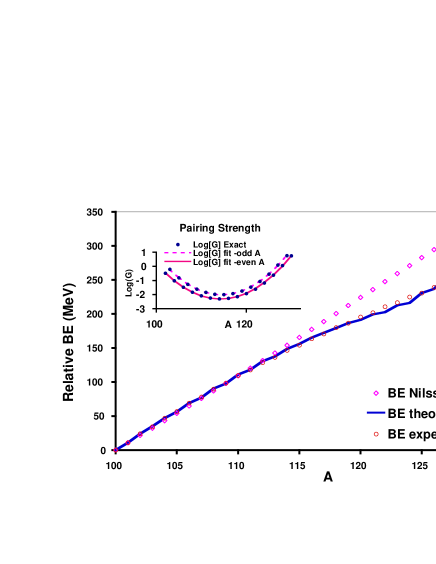
Figure 1: The solid line gives the binding energies of the Sn isotopes relative to that of the ¹⁰⁰Sn core. The single-particle energy scale is set by the binding energy of ¹⁰¹Sn. The inset shows the fit to values of $G$ that reproduces the experimental data exactly. The two fitting functions are: $\log(G(A))=365.0584-6.4836A+0.0284A^{2}$ for even values of $A$ and $\log(G(A))=398.2277-7.0349A+0.0307A^{2}$ for odd values of $A$. The Nilsson BE energy is the lowest energy of the non-interacting system.

We now turn to our results for the binding energies and $\log(G)$ values within the Nilsson plus extended pairing model for three isotopic chains: ^100-130Sn, ^152-181Yb, and ^181-202Pb. Figure 1 shows the results for the ^100-130Sn isotopes. Calculations for the pairing strength G were carried out for the ^102-130Sn isotopes within the 50-82 neutron shell. Once this was done, a quadratic polynomial fit of the $\log(G)$ values for even and odd $A$ was determined. By doing this we were able to fit two sets of 14 data points with two 3 parameter expressions. Overall the results are very good for the lower and middle part of the 50-82 neutron shell. Even though a particle-hole symmetry can be seen from the $\log(G)$ inset, there is a discrepancy between the two as one moves towards the upper part of the shell. This discrepancy is due to the shell closure, the single-particle level structure, and the Pauli blocking for odd A nuclei.

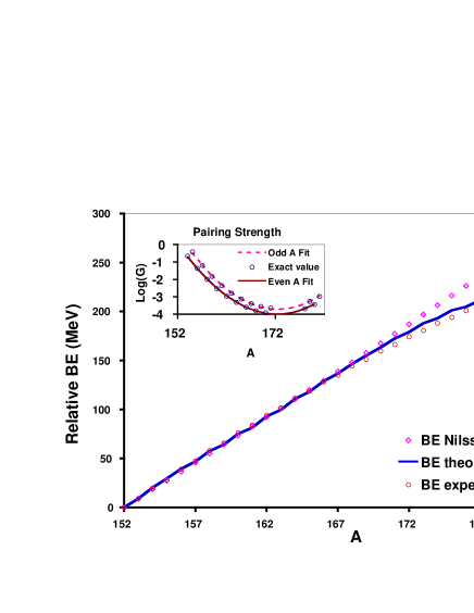
Figure 2: The solid line gives the binding energies of Yb isotopes relative to that of the ¹⁵²Yb core. The single-particle energy scale is set from the binding energy of ¹⁵³Yb. The inset shows the fit to values of $G$ that reproduce exactly the experimental data. The two fitting functions are: $\log(G(A))=662.2247-7.7912A+0.0226A^{2}$ for even values of $A$ and $\log(G(A))=716.3279-8.4049A+0.0244A^{2}$ for odd values of $A$. The Nilsson BE energy is the lowest energy of the non-interacting system.

Figure 2 shows our results for the ^154-161Yb isotopes. We test the predictive power of the model on the ^172-177Yb isotopes. In this case calculations of the pairing strength G are carried out only for the ^{154-171,178-181}Yb isotopes and not for the ^172-177Yb isotopes that are in the middle of the model space and thus are more computationally involved. This is a fit of two sets of 11 data points with two 3 parameter expressions. Then from the obtained quadratic polynomial fit to the $\log(G)$ values we calculate the theoretical values of the binding energy for these nuclei as shown in Figure 2. This prediction is very good when compared to the experiment. Thus, based on experimental data of the nuclei in the upper and lower part of the shell and a $\log(G)$ fit to this data we can make a reasonable estimate for the mid-shell nuclei. Therefore, the model has a good predictive power.

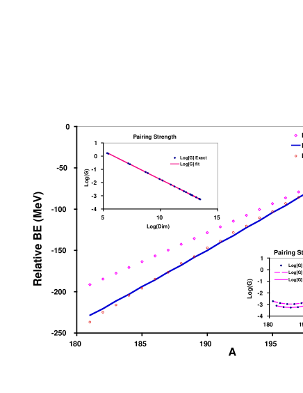
Figure 3: The solid line gives the binding energy for the Pb isotopes relative to the ²⁰⁸Pb nucleus. The insets show the fit to the values of $G$ that reproduce exactly the experimental data using a ¹⁶⁴Pb core. The lower inset shows the two fitting functions: $\log(G(A))=382.3502-4.1375A+0.0111A^{2}$ for even values of $A$ and $\log(G(A))=391.6113-4.2374A+0.0114A^{2}$ for odd values of $A$. The upper inset shows a fit to $G(A)$ that is inversely proportional to the size of the model space, ($\dim(A)$), that is valid for even as well as odd values of $A$: $G(A)=366.7702/\dim(A)^{0.9972}$. The Nilsson BE energy is the lowest energy of the non-interacting system.

The next Figure 3 shows results for the ^181-202Pb isotopes that were studied in the same way as the Sn and Yb isotopes. In the calculations for these Pb isotopes, however, the binding energy that was used is relative to that for ²⁰⁸Pb which was set to zero, but the core nucleus was chosen to be ¹⁶⁴Pb. Note that for the Yb and Sn isotopes the core nucleus was also the binding energy reference nucleus (¹⁰⁰Sn and ¹⁵²Yb). In contrast, the calculation for the Pb-isotopes was different because the core nucleus (¹⁶⁴Pb) and the binding energy reference nucleus (²⁰⁸Pb) are different. We again have good quadratic fit to $\log(G)$ as function of $A$.

The fact that there is a correlation between the pairing strength $G$ and the size of the model space reflected in the minimum of $G$ that is at the maximal model space dimension prompted us to study $G(A)$ as function of the model space dimension $\dim(A)$. In this respect, a remarkable results is shown in Figure 3. In this case the pairing strength $G(A)$ for all the 21 nuclei (A=$181-202$) was fit by a two parameter function $G(A)=\alpha/[\dim(A)]^{\beta}$ with the values of the parameters taken to be $\alpha=366.7702$ and $\beta=0.9972$. This function is inversely proportional to the dimensionality of the model space $\dim(A)$. Unfortunately, this is not the case for the other two isotopic chains. For example, in Figure 4 a $\log-\log$ plot is shown for the Sn nuclei.

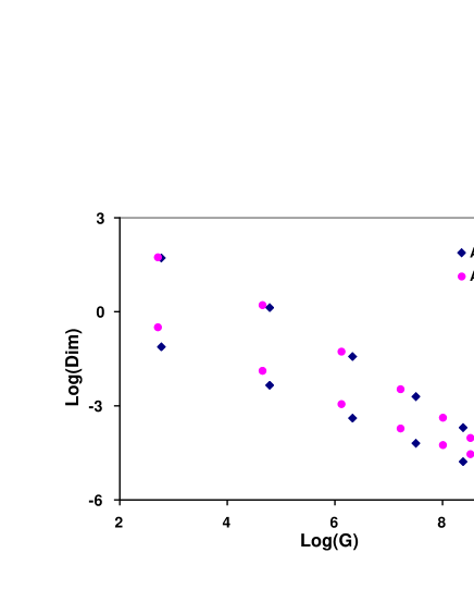
Figure 4: Results for $\log(G)$ versa $\log(\dim)$ for the Sn nuclei.

It is unlikely that the linear relation between $\log(G)$ and $\log(\dim(A))$ for the Pb isotopes is due to the difference between the core and binding energy reference nucleus. What is more likely is that this is due to the fact that in these cases the model space dimensions are sufficiently large to result in a limiting form for the effective pairing strength. Another reason might be that the single-particle energies and the Pauli blocking mechanism are such that the even and odd parabolas of $\log(G(A))$ produce a linear $\log-\log$ structure.

In the light of the above, it seems that the next step should be a study that tracks the results as a function of the increasing size of the model space to confirm or refute the $\log-\log$ relation. Such a study could also address other questions such as the effect of the core binding energy as a function of the deformation that is used in the Nilsson model to derive the single-particle energies. Using a Woods-Saxon potential or other methods to generate more realistic single-particle energies is another opportunity for further studies.

In conclusion, we have studied binding energies of nuclei in three isotopic chains: ^100-130Sn, ^152-181Yb, and ^181-202Pb within the recently proposed extended pairing model FirstPaper by using Nilsson single-particle energies as the input mean-field energies. Overall, the results suggest that the model is applicable to well-deformed nuclei if the pairing strength is allowed to change as a (smooth) function of the nucleon number $A$. The remarkably similar behavior of $\log(G)$ for even and odd $A$ values seems to suggest that there may be a single $\log(G)$ function that bifurcates into an even-$A$ and an odd-$A$ branch when the fermion dynamics is restricted to hard boson pairs only and Pauli blocking is applied to exclude levels populated by the unpaired fermion.

Support provided by the U.S. National Science Foundation (0140300), the Natural Science Foundation of China (10175031), and the Education Department of Liaoning Province (202122024) is acknowledged.

References

- (1) F. Pan, V. G. Gueorguiev, and J. P. Draayer, to appear in Phys. Rev. Lett. (2004), (nucl-th/0311075).
- (2) C. T. Black, D. C. Ralph, and M. Tinkham, Phys. Rev. Lett. 76, 688 (1996); D. C. Ralph, C. T. Black, and M. Tinkham, Phys. Rev. Lett. bf 78, 4087(1996).
- (3) F. Pan, J. P. Draayer, and W. E. Ormand, Phys. Lett. B422, 1 (1998); F. Pan and J. P. Draayer, Phys. Lett. B442, 7 (1998); F. Pan, J. P. Draayer, and Lu Guo, J. Phys. A: Math. Gen. 33, 1597 (2000); F. Pan and J. P. Draayer, J. Phys. A: Math. Gen. 33, 9095 (2000); J. Dukelsky, C. Esebbag, and P. Schuck, Phys. Rev. Lett. 87, 066403 (2001); J. Dukelsky, C. Esebbag, and S. Pittel, Phys. Rev. Lett. 88, 062501 (2002); H. -Q. Zhou, J. Links, R. H. McKenzie, and M. D. Gould, Phys. Rev. B 65, 060505(R) (2002).
- (4) F. Pan and J. P. Draayer, Ann. Phys. (NY) 271, 120 (1999).
- (5) R. W. Richardson, Phys. Lett. 3, 277 (1963); R. W. Richardson, Phys. Lett. 5, 82 (1963); R. W. Richardson and N. Sherman, Nucl. Phys. 52, 221 (1964).
- (6) S. Rombouts, D. Van Neck, and J. Dukelsky, nucl-th/0312070.
- (7) J. R. Nix and K. L. Kratz, Atomic Data Nucl. Data Tables 66, 131 (1997); P. Möller, J. R. Nix, W. D. Myers, and W. J. Swiatecki, Atomic Data Nucl. Data Tables 59, 185-381 (1995).
- (8) G. Audi, et al., Nucl. Phys. A624, 1 (1997).