Viscosity and Thermalization

Abstract

I solve a Relativistic Navier Stokes Model assuming boost invariance and rotational symmetry. I compare the resulting numerical solutions for two limiting models of the shear viscosity. In the first model the shear viscosity is made proportional to the temperature. Thus, $\eta\propto T/\sigma_{0}$ where $\sigma_{0}$ is some fixed cross section (perhaps $\sigma_{0}\sim\Lambda_{QCD}^{-2}$) . This viscosity model is typical of the classical Boltzmann simulations of Gyulassy and Molnar. In the second model the shear viscosity is made proportional to $T^{3}$. This model is typical of high temperature QCD. When the initial mean free path of the $T^{3}$ model is four times larger than the $T/\sigma_{0}$ model, the two models of viscosity produce the same radial flow. This result can be understood with simple scaling arguments. Thus, the large transport opacity needed in classical Boltzmann simulations is in part an artifact of the fixed scale $\sigma_{0}$ in these models.

1. Motivation: The observation of elliptic flow is one of the most striking results the heavy ion program [1]. In mid-peripheral collisions the azimuthal anisotropy of the produced particles $v_{2}(p_{T})\equiv\left\langle\cos(2\phi)\right\rangle_{p_{T}}$ rises linearly as a function of transverse momentum up to $p_{T}\sim 1.5\,\mbox{GeV}$ and then flattens and maintains a constant value of approximately $15\%$. Ideal hydrodynamics provides an economical description of the observed elliptic flow for transverse momentum below $1.5\,\mbox{GeV}$ [2]. However, ideal hydrodynamics assumes that the transport mean free path $\ell_{mfp}$ path is so small that viscous terms can be neglected. Simple estimates indicate that that in heavy ion collisions this assumption is marginal. It is hoped that $\ell_{mfp}/L$ is of order $\sim~{}1/5$ and that some semblance of an equilibrium QGP plasma will be formed. For $\ell_{mfp}/L\sim 1/5$ viscous hydrodynamics should provide a semi-quantitative guide to the evolution of the system. Viscous hydrodynamics should then explain the systematics of the elliptic flow measurements.

Elliptic flow was studied in the fully non-equilibrium framework of classical kinetic theory by Gyulassy and Molnar [3]. These authors varied the cross section between classical particles and computed the resulting elliptic flow. The results are surprising. First, the full kinetic theory reproduces the full shape of the $v_{2}(p_{T})$ curve. In particular the kinetic theory describes the linear rise with transverse momentum (as expected from hydrodynamics) and the subsequent flattening of $v_{2}(p_{T})$ . The first viscous correction to the thermal distribution function clarifies this transition from the hydrodynamic to the kinetic regime [4]. In spite of this success, these classical Boltzmann simulations suggest that hydrodynamics is not responsible for the observed $v_{2}$. The cross sections needed to reproduce the observed elliptic flow are $\approx 10\,\mbox{mb}$. With such cross sections the initial momentum degradation length is approximately four times smaller than the thermal wavelength. This seems impossible.

However, several differences between between QCD and these classical cascade models should be noted. First, the classical cascade preserves particle number. Second, the classical simulation have a fixed scale $\sigma_{0}$. This is not so unreasonable – perhaps $\sigma_{0}$ is $\Lambda_{QCD}^{2}$. To understand the implications of this fixed scale let us estimate the temporal dependence of the viscosity in different situations.

In the perturbative quark gluon plasma the shear viscosity is proportional $T^{3}$ as given by dimension. Thus the ratio of the shear viscosity to the entropy $\eta/s$ is a constant up to logarithms. In a classical massless gas with constant cross sections the shear viscosity is given by $\eta=1.264\,T/\sigma_{0}$ Thus the temperature dependence of the shear viscosity in the classical model [3] differs from high temperature QCD. Simple scaling arguments indicate that a model with a constant cross section is unlikely to thermalize. For a Bjorken expansion, the condition for hydrodynamics to be valid is: $\Gamma_{s}/\tau\ll 1$ where where $\Gamma_{s}$ is the sound attenuation length $\frac{4}{3}\eta/(e+p)$ .

Next, I estimate how $\Gamma_{s}/\tau$ evolves as a function of time during a Bjorken expansion for the two limiting models of viscosity discussed above. For a Bjorken expansion $T\propto 1/\tau^{1/3}$ and $n\propto 1/\tau$. Then, when the viscosity is proportional to $T^{3}$ we find that the system comes closer to equilibrium as a function of time

$$\frac{\Gamma_{s}}{\tau}\sim\frac{1}{\tau T}\sim\frac{1}{\tau^{2/3}} \mbox{(1D Bjorken with $\eta\propto T^{3}$)}.$$

In contrast for a classical gas with conserved particle number $e+p=4\,nT$ and constant cross section the degree of thermalization remains constant as a function of time

$$\frac{\Gamma_{s}}{\tau}\sim\frac{1}{\tau n\sigma_{0}}\sim\mbox{Const} \mbox{ (1D Bjorken $\eta\propto T/\sigma_{0}$) }.$$

Similar instructive arguments may be given when the system expands in three dimensions. The conclusion remains the same. When the viscosity is proportional to $T^{3}$ the system is much more likely to thermalize than when other scales such as $\sigma_{0}$ and $\Lambda_{QCD}$ enter the problem.

2. Viscous Solutions. It has been understood for some time that the relativistic Navier stokes equations can not be solved directly. However, this problem is cosmetic rather than fundamental in nature [5]. A myriad of different hydrodynamic models [6, 7] can be solved numerically with considerable effort [8]. These models all give the same solution up to corrections which are proportional to $\left(\Gamma_{s}/\tau\right)^{2}$. The stress energy tensor is always close to its canonical form $T^{ij}\sim\eta\,\left(\partial^{i}v^{j}+\partial^{j}v^{i}-\frac{2}{3}\delta^{ij}\,\partial_{l}v^{l}\right)$. These model equations have no greater validity than the Navier Stokes equation. The hydrodynamic model used here was inspired by a model with appealing mathematical structure due to Ottinger [6].

First, I solve a Navier Stokes Model (the Ottinger Model [6]) assuming boost invariance and radial symmetry. The initial conditions are taken from P. Kolb’s inviscid hydrodynamic calculations [9] which reproduces the observed spectra and multiplicity. The viscosity is made proportional to the entropy  $\eta/s=1/5$. The viscous solution is compared with the inviscid (Euler) solution shown in Fig. 1.

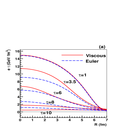
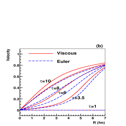
Figure 1: A comparison of the viscous and inviscid (Euler) solutions for a Bjorken expansion with radial symmetry. The initial conditions are from P. Kolb’s hydrodynamic model [9]. The equation of state is $p=\frac{1}{3}e$. The viscosity is proportional to the entropy $\eta/s=\frac{1}{5}$. (a) The energy density multiplied by $\tau$ for various times (b) The fluid velocity for various times.

Examine the energy density in Fig. 1(a). First the viscous solution does less longitudinal work since the longitudinal pressure is reduced by the longitudinal expansion (see e.g. [4]). Consequently, the energy density initially decreases more slowly for the viscous case. However, the transverse pressure is increased by longitudinal expansion. This causes the transverse flow to rise more rapidly in the viscous case as seen in Fig. 1(b). This larger transverse flow velocity subsequently causes the energy density to fall more rapidly in the viscous case. By a time of $\approx 6\,\mbox{fm}$ the viscous and inviscid solutions are similar. In summary, viscous corrections do not integrate to yield an order one change to the inviscid flow.

Next, I compare two simple models for the viscosity. The first model for the viscosity is taken from a classical ideal gas with a constant cross sections. In this case $\eta=1.264\frac{T}{\sigma_{0}}$ with $\sigma_{0}=10\,\mbox{mb}$. This model of the viscosity has been studied within the domain of kinetic theory by Gyulassy and Molnar [3].

The second model for the viscosity is referred to as the Minimal Model below. In this model we take

$$\eta=\left\{\begin{array}[]{lc}\rm 1.264\,\frac{T}{\sigma_{0}}&\mbox{ for }e<e_{c}\\ \rm\frac{1}{5}\,s&\mbox{ for }e>e_{c}\end{array}\right.$$ (1)

where $e_{c}=1\,\mbox{GeV/fm}^{3}$ and $\sigma_{0}=10\,\mbox{mb}$. This model of the shear viscosity has $\eta\propto T^{3}$ for high temperatures but has a fixed scale $\sigma_{0}$ (i.e. $\Lambda_{QCD}^{-2}$) at low temperatures. The shear viscosity of the Minimal Model is always larger than the fixed cross section model.

The viscous hydrodynamic solutions to these models are illustrated in Fig.  2. The two models of viscosity give approximately

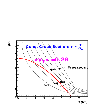
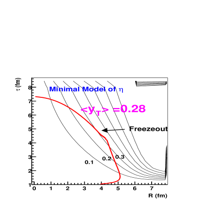
Figure 2: A comparison of two models of the shear viscosity. In the first model the shear viscosity $\eta=1.264T/\sigma_{0}$. The minimal model of viscosity is described in the text and has $\eta\propto T^{3}$ when the energy density exceeds $1.0\,\mbox{GeV/fm}^{3}$. In both case $p=\frac{1}{3}e$. The thin lines are lines of constant transverse rapidity with values $0.1,\,0.2,\,0.3\,...$ The thick line labeled Freezeout is where the viscous “correction” is half of the pressure. $\left\langle y_{T}\right\rangle$ denotes the entropy weighted mean transverse rapidity along the freezeout curve.

the same solution although the viscosity in the Minimal Model is initially four times larger than the fixed cross section model. Eventually, the viscosity becomes large and the system freezes out. The curve labeled ”freezeout” indicates when the viscous correction becomes equal to half of the hydrodynamic pressure. The mean transverse relativistic velocity $\left\langle y_{T}\right\rangle$ is calculated along the ”freezeout” curve using the Cooper-Frye formula and weighting each surface element by the entropy. The two models of the shear viscosity give approximately the same transverse flow as can be seen be comparing $\left\langle y_{T}\right\rangle$ in each case. Thus the large transport opacity needed in classical Boltzmann simulations is in part an artifact of the fixed scale $\sigma_{0}$ introduced into the problem.

References

- [1] For overview see, Zhangbu Xu, these proceedings.
- [2] For overview see, T. Hirano, these proceedings.
- [3] D. Molnar and M. Gyulassy, Nucl. Phys. A 697, 495 (2002).
- [4] D. Teaney, Phys. Rev. C 68, 034913 (2003).
- [5] L. Lindblom, gr-qc/9508058. R. Geroch, J. Math. Phys. 36, 4226 (1995).
- [6] H. C. Ottinger, Physica A 254 433 (1998).
- [7] W.Israel, Annals. Phys. 100, 310 (1976); R. Geroch and L. Lindblom, Phys. Rev. D 41, 1855 (1990);
- [8] D. Teaney, in preparation.
- [9] P.F. Kolb, P.Huovinen, U. Heinz, H. Heiselberg, Phys. Lett. B 500, 232 (2001); P. Huovinen, P.F. Kolb, U. Heinz, H. Heiselberg, Phys. Lett. B 503, 58 (2001).