Coulomb corrections for quasielastic (e,e’) scattering: eikonal approximation

Abstract

We address the problem of including Coulomb distortion effects in inclusive quasielastic $(e,e^{\prime})$ reactions using the eikonal approximation. Our results indicate that Coulomb corrections may become large for heavy nuclei for certain kinematical regions. The issues of our model are presented in detail and the results are compared to calculations of the Ohio group, where Dirac wave functions were used both for electrons and nucleons. Our results are in good agreement with those obtained by exact calculations.

,

1 Introduction

Nucleon knockout by electron scattering provides a powerful probe of the dynamics of nucleons in the nuclear medium. The transparency of the nucleus with respect to the electromagnetic probe makes it possible to study the entire nuclear volume. For light nuclei, the weakness of the electromagnetic interaction allows for a separation of the soft Coulomb distortion of the electron scattering process from the hard scattering event in which, to a very good approximation, a single virtual photon transfers energy and momentum to the nuclear constituents. Since the kinematic conditions of electron scattering can be varied easily, different aspects of the reaction mechanism can be tested. Under conditions in which a single nucleon receives most of the energy and momentum transfer, the quasifree electron-nucleon scattering process is emphasized.

Nucleon knockout from heavier nuclei is used to measure the single-nucleon spectral function in complex nuclei. At low excitation energy, exclusive measurements to discrete states of the residual nucleus provide information on quasiparticle properties, such as binding energies, spectroscopic factors, spreading widths and momentum distributions. The specific models used to extract the structure information can be tested by comparing parallel with nonparallel kinematics or by varying the ejectile energy. The spatial localization of specific orbitals also provides some sensitivity to possible density-dependent modifications of the electromagnetic properties of bound nucleons. The azimuthal dependence of the cross section and the recoil polarization of the ejectile can provide detailed tests of the reaction mechanism, which may be useful in delineating the role of two-body currents or in testing off-shell models of the current operator. Measurements at larger missing energy can provide information on the deep-hole spectral function or on multinucleon currents. Measurements at large missing momentum are sensitive to short-range and tensor correlations between nucleon pairs.

For heavier nuclei Coulomb corrections (CC) may become very large and affect the measured cross sections; this needs to be accounted for, if one aims at a quantitative interpretation of data. Here, we concentrate on the inclusive quasielastic scattering process $(e,e^{\prime})$, where only the scattered electron is observed. We will model this process as a knockout reaction where the nucleons are hit by the virtual photon emitted by the scattered electron.

Inclusive scattering provides information on a number of interesting nuclear properties:

-The width of the quasielastic peak allows a dynamical measurement of the nuclear Fermi momentum [1].

-The tail of the quasielastic peak at low energy loss and large momentum transfer gives information on high-momentum components in nuclear wave functions [2].

-The integral strength of quasielastic scattering, when compared to sum rules, tells us about the reaction mechanism and eventual modifications of nucleon form factors in the nuclear medium [3].

-The scaling properties of the quasielastic response allows to study the reaction mechanism [4].

-Extrapolation of the quasielastic response to $A=\infty$ provides us with a very valuable observable for infinite nuclear matter [5].

For heavier nuclei, these questions obviously can only be addressed once the Coulomb distortion of the electron waves is properly dealt with.

In this paper, we present an approximate treatment of electron CC for inclusive quasielastic $(e,e^{\prime})$ reactions modeled as a nucleon knockout process. In the plane-wave Born approximation (PWBA), the electrons are described as plane Dirac waves, which is a poor approximation for heavy nuclei with strong Coulomb fields. In a better approach, called eikonal distorted wave Born approximation (eDWBA), we use electron waves which are distorted by an additional phase and a change in the amplitude. This phase shift and the modification of the amplitude account for the enhanced momentum and a focusing effect which occurs when the electron approaches the strongly attractive nucleus.

Calculations with exact Dirac wave functions have been performed by Kim et al. [6] in the Ohio group and Udias et al. [7, 8]; the present eikonal approximation has the advantage that it is relatively simple to implement and that it avoids large computational costs. The eikonal method and its higher approximations, which can be obtained from an iterative procedure, is expected to lead to an asymptotic, rather than a convergent expansion [9]. Therefore, its use for the calculation of exclusive cross sections may be problematic according to Giusti and Pacati [10, 11], but the good agreement for the inclusive cross section with the exact calculations by Kim et al. seems to justify the method in this case. Additionally, the eikonal approximation used in [10, 11] is not equivalent to the approach used in this paper, since we do not calculate the electron wave phase shift from an expansion around the center of the nucleus. For exclusive cross sections, not only exact wave functions for the electrons are needed, but also an accurate description of the proton or neutron wave functions. In the inclusive case the fine details of the nuclear structure and final state interaction are not important, and the description of the unobserved knocked-out hadron can be rather cursory.

Various approximate treatments have been proposed in the past for the treatment of CC [10, 12, 13, 14, 15, 16, 17, 18, 19], and there is an extensive literature on the eikonal approximation [20, 21, 22, 23, 24]. In particular it has been shown that at lowest order, an expansion of the electron wave function in $\alpha Z$ leads to the well known effective momentum approximation (EMA) [9], which is explained in Sect. 2.2. The EMA has been used to correct Coulomb distortions for elastic electron scattering data or inelastic data to low lying states, although exact descriptions are readily available. For quasielastic $(e,e^{\prime})$ scattering a comparison of EMA calculations with numerical results from the ’exact’ DWBA calculation [25, 26] indicates a failure of the EMA [27].

We point out that the model of the nuclear structure used in this paper is relatively simple, since our focus is mainly on the electronic part of the problem, i.e. the influence of the Coulomb field on the electron wave function. Still, our simple model leads to satisfactory values for inclusive cross sections which are sufficient for our purpose. We also find that the EMA fails to account for CC for quasielastic $(e,e^{\prime})$. This observation is discussed in detail in Sect. 3.

2 Models and approximations

2.1 Effective momentum approximation

The accurate description of the electrostatic potential of the nucleus is an important ingredient for the calculation of CC. In a simplified classical picture, the electron hits mostly the outer region of the nucleus. This implies that for heavy nuclei like lead with a radius of approximately $6\,\mbox{fm}$, the kinetic electron energy is increased in this region by about 20 MeV, which is a non negligible modification when the electron energy lies in the range of a few hundreds of MeV. In the most naive picture, the effective momentum approximation, one typically assumes that the nucleus is a homogeneously charged sphere with equivalent radius $R_{e}$. For highly relativistic particles in a potential $V$ with asymptotic momentum $\vec{k}$, one may neglect the mass of the particle ($|E-V|,|\vec{k}\,|\gg m$), such that the energy-momentum relation reduces to ($\hbar=c=1$)

$$(E-V)^{2}=\vec{k}^{\,2}+m^{2}\,\rightarrow\,E-V=k,\,k=|\vec{k}|.$$ (1)

Then the momentum shift $\Delta k$ of a highly relativistic electron in the region where it interacts with the nucleus follows from the potential energy of the electron inside the nucleus ($C=1$ at the surface or $C=3/2$ in the center)

$$\Delta k=C\frac{\alpha Z}{R_{e}},\quad C=1\ldots 3/2,\quad k^{\mbox{\scriptsize{eff}}}_{i,f}=k_{i,f}+\Delta k\,.$$ (2)

The standard EMA uses effective momenta corresponding to the central value of the Coulomb potential (C=3/2). The EMA cross section of the considered process is then calculated by using the plane wave approach, but with the electron momenta replaced by their corresponding effective values. In this way one accounts for the fact that the electron wave length is reduced in the relevant nuclear region. But due to the attractive Coulomb potential, the modulus of the initial (final) electron wave is also enhanced by a factor of $\sim F_{i}$ ($F_{f}$) inside the nuclear volume. The cross section is therefore multiplied additionally by a factor $F_{i}^{2}=(k^{\mbox{\scriptsize{eff}}}_{i}/k_{i})^{2}$ which accounts for the focusing of the incoming electron wave in the nuclear center. The cross section is not multiplied by $F_{f}^{2}=(k^{\mbox{\scriptsize{eff}}}_{f}/k_{f})^{2}$, because this factor is already contained in the artificially enhanced phase space factor of the outgoing electron.

In order to be more explicit, we mention that in the plane wave Born approximation, the cross section for inclusive quasielastic electron scattering can be written by the help of the total response function $S_{total}$ as

$$\frac{d^{2}\sigma_{{}_{PWBA}}}{d\Omega_{f}d\epsilon_{f}}=\sigma_{Mott}\times S_{total}(|\vec{q}\,|,\omega,\Theta_{e}),$$ (3)

where the Mott cross section is given by

$$\sigma_{Mott}=4\alpha^{2}\cos^{2}(\Theta_{e}/2)\epsilon_{f}^{2}/q_{\mu}^{4}.$$ (4)

Here, $\alpha$ is the fine-structure constant, $\Theta_{e}$ is the electron scattering angle, $\vec{q}=\vec{k}_{i}-\vec{k}_{f}$ is the momentum transfer given by the initial and final electron momentum, $\omega=\epsilon_{i}-\epsilon_{f}$ is the energy transfer given by the initial and final electron energy, and the four-momentum transfer squared is given by $q_{\mu}^{2}=\omega^{2}-\vec{q}^{\,2}$.

The Mott cross section remains unchanged when it gets multiplied by the EMA focusing factors and the momentum transfer $q_{\mu}^{4}$ is replaced by its corresponding effective value, i.e. $F_{i}^{2}F_{f}^{2}/q_{\mu,\mbox{\scriptsize{eff}}}^{4}=1/q_{\mu}^{4}$. Therefore, the EMA cross section can also be obtained from (3) by leaving the Mott cross section unchanged and by replacing $S_{total}(|\vec{q}\,|,\omega,\Theta_{e})$ by the effective value $S_{total}(|\vec{k}_{i}^{\mbox{\scriptsize{eff}}}-\vec{k}_{f}^{\mbox{\scriptsize{eff}}}|,\omega,\Theta_{e})$.

2.2 Eikonal approximation

We can take the local change in the momentum of the incoming particle with momentum $\vec{k}_{i}=k_{i}\hat{k}_{i}$ into account approximately by modifying the plane wave describing the initial state of the particle by the eikonal phase $\chi_{1}(\vec{r})$

$$e^{i\vec{k}_{i}\vec{r}}\,\rightarrow\,e^{i\vec{k}_{i}\vec{r}+i\chi_{1}(\vec{r})}\,,$$ (5)

where

$$\chi_{1}(\vec{r})=-\int\limits_{-\infty}^{0}V(\vec{r}+\hat{k}_{i}s)ds=-\int\limits_{-\infty}^{z}V(x,y,z^{\prime})dz^{\prime}\,$$ (6)

if we set $\vec{k}_{i}=k_{z}^{i}\hat{{\bf{e}}}_{z}$. As desired, the $z$-component of the momentum then becomes

$$p_{z}=-i\partial_{z}e^{ik_{z}^{i}z+i\chi_{1}}=(k_{z}^{i}-V)e^{ik_{z}^{i}z+i\chi_{1}}.$$ (7)

The final state wave function is constructed analogously

$$e^{i\vec{k}_{f}\vec{r}-i\chi_{2}(\vec{r})},$$ (8)

where

$$\chi_{2}(\vec{r})=-\int\limits_{0}^{\infty}V(\vec{r}+\hat{k}_{f}s^{\prime})ds^{\prime}\,.$$ (9)

For the sake of simplicity, we consider spinless electrons in Sects. 2.1-2.4. In our actual calculations spin is included. The spatial part of the free electron current (which interacts via photon exchange with the particles inside the nucleus)

$$\vec{j}_{{}_{PW}}=-ie[e^{-i\vec{k}_{f}\vec{r}}\vec{\nabla}e^{i\vec{k}_{i}\vec{r}}-(\vec{\nabla}e^{-i\vec{k}_{f}\vec{r}})e^{i\vec{k}_{i}\vec{r}}]=e(\vec{k}_{i}+\vec{k}_{f})e^{i(\vec{k}_{i}-\vec{k}_{f})\vec{r}}$$ (10)

is replaced by

$$\vec{j}_{{}_{EIK}}=-ie[e^{-i\vec{k}_{f}\vec{r}+i\chi_{2}(\vec{r})}\vec{\nabla}e^{i\vec{k}_{i}\vec{r}+i\chi_{1}(\vec{r})}-(\vec{\nabla}e^{-i\vec{k}_{f}\vec{r}+i\chi_{2}(\vec{r})})e^{i\vec{k}_{i}\vec{r}+i\chi_{1}(\vec{r})}]=$$

$$e(\vec{k}_{i}+\vec{k}_{f}+\vec{\nabla}\chi_{1}-\vec{\nabla}\chi_{2})e^{i(\vec{k}_{i}-\vec{k}_{f})\vec{r}+i(\chi_{1}+\chi_{2})}\,,$$ (11)

where $e$ is the charge of the electron. The spatial part of the electron current now contains the additional eikonal phase, and the prefactor contains gradient terms of the eikonal phase which represent essentially the change of the electron momentum due to the attraction of the electron by the nucleus.

So far we have only considered the modification of the phase of the wave function, and for many applications this is a sufficient approximation. It has been applied to elastic high energy scattering of Dirac particles in an early paper by Baker [28]. However, the method leads, e.g. for quasielastic scattering of electrons on lead with initial energy $\epsilon_{i}=300$ MeV and energy transfer $\omega=100$ MeV, to errors up to 50% in the cross sections. The reason is that also the amplitude of the incoming and outgoing particle wave functions is changed due to the Coulomb attraction, as mentioned above. This fact can be related to the classical observation that an ensemble of negatively charged test particles approaching a nucleus is focused due to its attractive potential. Below, we give a simple classical treatment of this fact which illustrates the basic properties of the phenomenon. A semiclassical discussion of the focusing factor can also be found in [9].

2.2.1 The focusing factor

The focusing factor can be derived approximately from a classical toy model according to Fig. (1). We consider the trajectories of an ensemble of highly relativistic particles approaching the nucleus in the center of the coordinate system in $z$-direction with an impact parameter between $b_{0}$ and $b_{0}+db_{0}$. The longitudinal velocity of the particles can be taken as the speed of light, since the particles are highly relativistic and the change of the velocity in transverse direction causes only a second order effect to the longitudinal component. Therefore we have $z(t)=t$, $r(t)=\sqrt{b_{0}^{2}+t^{2}}$, keeping in mind that the impact parameter can be considered as constant at this stage of our approximation. The density of the particles at $z$ is increased by a focusing factor $f$ which is given by the ratio of the area of two annuli with radii $b_{0},b_{0}+db_{0}$ and $b(b_{0},z),b(b_{0}+db_{0},z)$:

$$f^{-1}(b_{0},z)=\frac{\partial b(b_{0},z)}{\partial b_{0}}\frac{b(b_{0},z)}{b_{0}}.$$ (12)

We will calculate now $b(b_{0},z)$ for the screened potential

$$V_{s}(r)=-\frac{\alpha Z}{\sqrt{r^{2}+R^{2}}},$$ (13)

since in this case a simple study of the problem and its most important properties is possible.

Figure 1: Electrons incident on an nucleus with impact parameter $b_{0}$.

The force $F_{T}$ acting on the particle in transverse direction is given by

$$F_{T}=-\frac{b}{r}\frac{\partial V(r)}{\partial r}\sim-\frac{\alpha Zb_{0}}{\sqrt{r^{2}+R^{2}}^{3}},$$ (14)

whereas the ”transverse mass” is given by the energy $E$ $(c=1)$. Therefore we obtain for the transverse acceleration

$$\dot{v}_{T}=-\frac{\alpha Z}{E}\frac{b_{0}}{\sqrt{t^{2}+b_{0}^{2}+R^{2}}^{3}},$$ (15)

and

$$v_{T}(t)=-\frac{\alpha Z}{E}\frac{b_{0}}{b_{0}^{2}+R^{2}}\frac{t+\sqrt{t^{2}+b_{0}^{2}+R^{2}}}{\sqrt{t^{2}+b_{0}^{2}+R^{2}}}=$$

$$-\frac{\alpha Z}{E}\frac{b_{0}}{b_{0}^{2}+R^{2}}\frac{t+\sqrt{r^{2}+R^{2}}}{r^{2}+R^{2}}.$$ (16)

From $v_{T}(t\rightarrow\infty)=-\frac{2\alpha Z}{E}\frac{b_{0}}{b_{0}^{2}+R^{2}}$ we obtain for a pure Coulomb field $(R\ll b_{0})$ the well-known transverse momentum transfer

$$\Delta k_{T}=\frac{2\alpha Z}{b_{0}}.$$ (17)

Furthermore, we obtain from (16)

$$b(z)=b_{0}-\frac{\alpha Z}{E}\frac{b_{0}(z+\sqrt{r^{2}+R^{2}})}{b_{0}^{2}+R^{2}},$$ (18)

The focusing factor is then given by $(\beta=\alpha Z/E)$

$$f^{-1}=\Bigl{(}1-\frac{z+\sqrt{r^{2}+R^{2}}}{b_{0}^{2}+R^{2}}\beta\Bigr{)}\times$$

$$\Bigl{(}1-\Bigl{(}\frac{z+\sqrt{r^{2}+R^{2}}}{b_{0}^{2}+R^{2}}-\frac{2b_{0}^{2}(z+\sqrt{r^{2}+R^{2}})}{(b_{0}^{2}+R^{2})^{2}}+\frac{b_{0}^{2}}{(b_{0}^{2}+R^{2})\sqrt{r^{2}+R^{2}}}\Bigr{)}\beta\Bigr{)}.$$ (19)

Since our calculation is not exact, we keep only the relevant first order in $\beta$ in (19). For the focusing factor in the center of the nucleus follows

$$f(0)=\Bigl{(}1-\frac{\beta}{R}\Bigr{)}^{-2}\sim\Bigl{(}1-\frac{V(0)}{E}\Bigr{)}^{2}\sim(k^{\prime}_{i}/k_{i})^{2},$$ (20)

i.e. one obtains the focusing factor used in the effective momentum approximation, where the increased density near the nucleus is taken into account by multiplying the wave function by a suitable factor $\sim f^{1/2}$. In (20), $k_{i}=E/c$ denotes the asymptotic momentum of the highly relativistic incident particles, whereas $k^{\prime}_{i}$ is the momentum of a particle with impact parameter $b_{0}=0$ in the center of the nucleus, which is given by $k^{\prime}_{i}=k_{i}+\alpha Z/(Rc)$. c is the speed of light. The amplitude of the wave function is then correctly normalized in the region of the nucleus, where the nucleon knockout process is taking place. The discussion given above is only classical, but it is sufficient to show the most important features of the focusing effect. E.g., from (19) is it obvious that the amplitude of the wave function continues to increase on the rear side of the nucleus due to the deflection of the incoming particle wave.

Knoll [14] derived the focusing effect from a high energy partial wave expansion, following previous results given by Lenz and Rosenfelder [13, 18]. For the incoming particle wave expanded around the center of the nucleus he obtained:

$$\chi_{k}^{+}=e^{i\delta_{+}}(k^{\prime}/k)e^{i\vec{k^{\prime}}\vec{r}}\times$$

$$\{1+a_{1}r^{2}-2a_{2}\vec{k^{\prime}}\vec{r}+ia_{1}r^{2}\vec{k^{\prime}}\vec{r}+ia_{2}[(\vec{k^{\prime}}\times\vec{r})^{2}+\vec{\sigma}(\vec{k^{\prime}}\times\vec{r})]\}u_{k},$$ (21)

where $\vec{k^{\prime}}$ is parallel to $\vec{k}$, and where $\sigma$ acts on the spinor $u_{k}$ to describe spin dependent effects, which are very small in our cases of interest. An analogous equation holds for the distortion of the outgoing wave. The parameters $a_{1,2}$ depend on the shape of the potential. For a homogeneously charged sphere with radius $R_{s}$ they are given by

$$a_{1}=-\frac{\alpha Z}{6k^{\prime}R_{s}^{3}},\quad a_{2}=-\frac{3\alpha Z}{4k^{\prime 2}R_{s}^{2}}.$$ (22)

The increase of the amplitude of the wave while passing through the nucleus is given by the $-2a_{2}\vec{k^{\prime}}\vec{r}$-term. Taking our classical result for a screened potential leads to $a_{2}\sim\alpha Z/k^{\prime 2}R^{2}$, a result which cannot be compared directly to (22) due to the different shape of the potentials. Due to the fact that the amplitude of the wave function is smaller in the upstream side of the nucleus but larger by a similar amount on the downstream side, the influence of the $-2a_{2}\vec{k^{\prime}}\vec{r}$-term on the cross section in general is not very large. Minor effects can be observed for large scattering angles. Also the spin related term is of minor importance for highly relativistic electron energies.

The $a_{1}r^{2}$-term accounts for the decrease of the focusing also in transverse direction. For the cases of interest in this paper, it leads to 1-2 percent effects in the cross sections. Imaginary terms like $ia_{2}(\vec{k^{\prime}}\times\vec{r})^{2}$ describe the deformation of the wave front near the center of the nucleus. They could be obtained correspondingly by an expansion of the eikonal phase in that region, and $\delta_{+}$ is the eikonal phase in the center of the nucleus.

In the present work, the eikonal phase is obtained directly from an analytic expression as described in Sect. 2.2, whereas the focusing is calculated using Knoll’s results given above for a homogeneously charged sphere.

2.3 Electrostatic potential of the nucleus

For our present eikonal calculations, we use a potential energy of the electron of the form

$$(\alpha Z)^{-1}V(r)=-\frac{r^{2}+\frac{3}{2}R^{2}}{(r^{2}+R^{2})^{3/2}}-\frac{24}{25\pi}\frac{R^{2}R^{\prime}r^{4}}{(r^{2}+R^{\prime 2})^{4}}\,,$$ (23)

which goes over into a Coulomb potential for $r\rightarrow\infty$, and which is a good approximation for the potential generated by the Woods-Saxon-like charge distribution of a nucleus (see Fig. 2). $R^{\prime}$ can be used as an additional fit parameter. A good choice is $R^{\prime}=0.5174R_{e}$. Furthermore, expression (23) has the advantage that it is possible to derive an analytic expression for the eikonal phase, which is convenient when the eikonal phase has to be calculated numerically in a computer program.

The eikonal phase turns out to be divergent for a Coulomb-like potential, but it is possible to regularize the eikonal phase by subtracting a screening potential $\sim(r^{2}+a^{2})^{-1/2}$ with $a\gg R$ from (23), such that the potential falls off like $r^{-2}$ for large $r$. The divergence can then be absorbed in a constant divergent phase $\sim\log(a)$ without physical significance, when the limit $a\rightarrow\infty$ is taken. It is quite instructive to calculate the eikonal phase for the simple screened potential [29]

$$V_{1}(r)=-\frac{\alpha Z}{\sqrt{r^{2}+R^{2}}}\,,\quad V_{1}^{a}(r)=-\frac{\alpha Z}{\sqrt{r^{2}+R^{2}}}+\frac{\alpha Z}{\sqrt{r^{2}+a^{2}}}\,.$$ (24)

One obtains for a particle incident parallel to the z-axis for impact parameter $b$ ($r^{\prime 2}=b^{2}+z^{\prime 2}$)

$$\chi_{1}^{a}=\alpha Z\int_{-\infty}^{z}dz^{\prime}\,\Bigl{(}\frac{1}{\sqrt{r^{\prime 2}+R^{2}}}-\frac{1}{\sqrt{r^{\prime 2}+a^{2}}}\Bigr{)}=$$

$$\alpha Z\log\frac{(z+\sqrt{r^{2}+R^{2}})(b^{2}+a^{2})}{(z+\sqrt{r^{2}+a^{2}})(b^{2}+R^{2})},$$ (25)

where $r^{2}=b^{2}+z^{2}$, and therefore for the regularized eikonal phase

$$\chi_{1}=\lim_{a\to\infty}(\chi_{1}^{a}-\alpha Z\log(a))=\alpha Z\log\Bigl{(}\frac{z+\sqrt{r^{2}+R^{2}}}{b^{2}+R^{2}}\Bigr{)}.$$ (26)

which is defined up to a constant phase. Taking the gradient of $\chi_{1}$ in transverse direction

$$\frac{\partial\chi_{1}}{\partial b}=-\frac{\alpha Zb}{b^{2}+R^{2}}\frac{z+\sqrt{r^{2}+R^{2}}}{r^{2}+R^{2}},$$ (27)

gives for the transverse momentum transfer the same result as the classical expression (16). This illustrates the fact that the eikonal approximation also accounts for the transverse modification of the particle momentum. The charge density

$$\rho(r)=-\frac{1}{er}\partial^{2}_{r}(rV(r))$$ (28)

corresponding to the potential given by Eq. (23) satisfies

$$\langle\rho\rangle=eZ\,,$$ (29)

$$\langle r^{2}\rho\rangle=\frac{3}{5}R^{2}eZ\,,$$ (30)

i.e. we can indeed identify $R^{2}$ with the equivalent radius of a homogeneously charged sphere $R_{e}^{2}$ which is given approximately by

$$R_{e}=1.128A^{1/3}\,\mbox{fm}+2.24A^{-1/3}\,\mbox{fm}$$ (31)

for nuclei with $A>20$. $R_{e}$ can be related to the rms radius $R_{m}$ by

$$R_{m}^{2}=\frac{3}{5}R_{e}^{2}\,.$$ (32)

For a simple potential $\sim(r^{2}+R^{2})^{-1/2}$, the rms radius does not exist, since the corresponding charge distribution does not fall off fast enough.

The expressions necessary for the calculation of the eikonal phase for the potential (23) are given in the appendix.

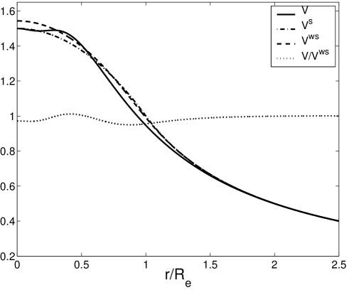
Figure 2: Comparison of different model potentials: Potential $V$ used in our calculations, potential $V^{s}$ generated by a homogeneously charged sphere with radius $R_{e}$ and potential generated by a corresponding Woods-Saxon charge distribution.

2.4 Scattering cross section

For the sake of notational simplicity and in order to give a transparent introduction to the method used for the calculation of the CC, we will neglect the dependence of the interactions on the spin and internal structure of the particles. Therefore, the particle wave functions are replaced by scalar fields in the following discussion. We call the positively charged particle the ’proton’, whereas the negatively charged particle is the ’electron’. The simplified scalar expression for the electron current can then be replaced by the correct Dirac current (43) in a straightforward way. The nucleon current which we used for our calculations is discussed below.

The lowest order transfer current of an electron with initial/final state wave function $\phi_{e}^{i,f}$ and a scalar (point-like) proton with initial/final state wave function $\phi_{p}^{i,f}$ is given by

$$j_{e}^{\mu}=+ie(\phi_{e}^{f\dagger}\partial^{\mu}\phi_{e}^{i}-\phi_{e}^{i}\partial^{\mu}\phi_{e}^{f\dagger})\,,$$ (33)

$$j_{p}^{\mu}=-ie(\phi_{p}^{f\dagger}\partial^{\mu}\phi_{p}^{i}-\phi_{p}^{i}\partial^{\mu}\phi_{p}^{f\dagger}).$$ (34)

For the scattering cross section of an electron with initial and final momentum $k_{i}^{\mu}=(\epsilon_{i},\vec{k}_{i})$, $k_{f}^{\mu}=(\epsilon_{f},\vec{k}_{f})$ off a proton with momenta $p_{i}^{\mu}=(E_{i},\vec{p}_{i})$, $p_{f}^{\mu}=(E_{f},\vec{p}_{f})$ we obtain in Born approximation the second order contribution in the coupling constant $e$ to the differential cross section ($e^{2}=4\pi\alpha$):

$$d\sigma=\frac{1}{4\epsilon_{i}E_{i}|v^{e}_{i}-v^{p}_{i}|}\Bigl{(}\frac{d^{3}k_{f}}{2\epsilon_{f}(2\pi)^{3}}\frac{d^{3}p_{f}}{2E_{f}(2\pi)^{3}}\Bigr{)}$$

$$\times(2\pi)^{4}\delta^{(4)}(k_{i}+p_{i}-k_{f}-p_{f})|M|^{2},$$ (35)

where the matrix element $M$ is given by the product of the currents and the photon propagator

$$M=e^{2}\frac{(k_{i}+k_{f})_{\mu}(p_{i}+p_{f})^{\mu}}{(k_{i}-k_{f})^{2}}.$$ (36)

The corresponding expression for the physical situation where electrons and nucleons are treated as particles with spin can be found, e.g., in [8].

Since we consider proton knockout by highly relativistic electrons from a nucleus at rest, the velocity in the flux term $|v^{e}_{i}-v^{p}_{i}|$ will be set to the speed of light.

If the initial proton is in a bound state with wave function

$$\phi_{p}^{i}(\vec{r},t)=(2\pi)^{-3/2}\int d^{3}q\,\hat{\psi}(\vec{q}\,)e^{i(\vec{q}\vec{r}-E_{i}t)},$$ (37)

the transition probability is replaced by $(p_{i}^{\mu}=(E_{i},\vec{q}\,))$

$$(2\pi)^{4}\delta^{(4)}(k_{i}+p_{i}-k_{f}-p_{f})|M|^{2}\rightarrow$$

$$2\pi\delta(\epsilon_{i}+E_{i}-\epsilon_{f}-E_{f})$$

$$\times\Bigl{|}\,e^{2}\int d^{3}q\int d^{3}r\,\frac{(k_{i}+k_{f})_{\mu}(p_{i}+p_{f})^{\mu}}{(E_{i}-E_{f})^{2}-(\vec{q}-\vec{p}_{f})^{2}}\,\hat{\psi}(\vec{q})\,e^{i(\vec{k}_{i}+\vec{q}-\vec{k}_{f}-\vec{p}_{f})\vec{r}}\,\Bigl{|}^{2}\rightarrow$$

$$(2\pi)^{4}\delta(\epsilon_{i}+E_{i}-\epsilon_{f}-E_{f})$$

$$\times\Bigl{|}\,e^{2}\frac{(k_{i}+k_{f})_{\mu}(2p_{f}+k_{f}-k_{i})^{\mu}}{(k_{i}-k_{f})^{2}}\hat{\psi}(\vec{k_{f}}+\vec{p_{f}}-\vec{k_{i}})\,\Bigr{|}^{2}.$$ (38)

In the distorted wave Born approximation, the presence of the Coulomb field is taken into account by using exact wave functions of the particles in the Coulomb field. In the eDWBA, these wave functions are replaced by their eikonal approximation. Therefore, the electron current is modified by the eikonal phase and due to the focusing of the electron wave. For electrons with potential energy $V(r)$ in the central Coulomb field of the nucleus we must replace

$$\int d^{3}q\int d^{3}r\,\frac{(k_{i}+k_{f})_{\mu}(p_{i}+p_{f})^{\mu}}{(E_{i}-E_{f})^{2}-(\vec{q}-\vec{p}_{f})^{2})}\,\hat{\psi}(\vec{q})\,e^{i(\vec{k}_{i}+\vec{q}-\vec{k}_{f}-\vec{p}_{f})\vec{r}}$$ (39)

by

$$\int d^{3}q\int d^{3}r\,\frac{(\tilde{k}_{i}+\tilde{k}_{f})_{\mu}(p_{i}+p_{f})^{\mu}}{(E_{i}-E_{f})^{2}-(\vec{q}-\vec{p}_{f})^{2})}\,\hat{\psi}(\vec{q})\,f(\vec{r})e^{i(\vec{k}_{i}+\vec{q}-\vec{k}_{f}-\vec{p}_{f})\vec{r}+i\chi(\vec{r})},$$ (40)

where

$$\tilde{k}_{i}^{\mu}=(\epsilon_{i}-V(r),\vec{k}_{i}+\vec{\nabla}\chi_{1})\,,$$ (41)

$$\tilde{k}_{f}^{\mu}=(\epsilon_{f}-V(r),\vec{k}_{f}-\vec{\nabla}\chi_{2})$$ (42)

correspond to the modified electron current in the eikonal approximation, and $f(\vec{r})$ denotes the focusing factor resulting from the incoming and outgoing particle wave function. The gradient and potential terms in the electron current are an artefact of our treatment of electrons as scalar particles. They appear in a similar fashion in the Gordon form of the electron current. The standard Dirac form of the current

$$j^{\mu}=e\bar{\Psi}\gamma^{\mu}\Psi,$$ (43)

can be split into a convective current and a spin current after some algebra by making use of the Dirac equation. One obtains

$$j^{\mu}=\frac{ie}{2m}\bigl{[}\bar{\Psi}\partial^{\mu}\Psi-(\partial^{\mu}\bar{\Psi})\Psi+\frac{2ie}{m}\bar{\Psi}\Psi A^{\mu}\bigl{]}+\frac{e}{2m}\partial_{\mu}[\bar{\Psi}\sigma^{\mu\nu}\Psi]\,.$$ (44)

The convective and the spin current are separately conserved and gauge invariant. But it is not advisable to use the Gordon form (44) in conjunction with the inexact eikonal approximation of the electron wave function, because the electron current is then described less accurately than by the standard expression (43).

It is now no longer possible to evaluate the coordinate space integral in a trivial way. As a first approximation we assume that the initial momentum (”missing momentum”) of the bound proton is given approximately by the external momenta, i.e.

$$\vec{q}=\vec{k}_{f}+\vec{p}_{f}-\vec{k}_{i}-\Delta\vec{q},\quad\Delta\vec{q}\sim 0.$$ (45)

Then we can expand

$$\Bigl{(}(\epsilon_{i}-\epsilon_{f})^{2}-(\vec{q}-\vec{p}_{f})^{2}\Bigr{)}^{-1}=$$

$$\Bigl{(}(\epsilon_{i}-\epsilon_{f})^{2}-(\vec{k}_{i}-\vec{k}_{f})^{2}-2(\vec{k}_{i}-\vec{k}_{f})\Delta\vec{q}-\Delta\vec{q}^{\,2}\,\Bigr{)}^{-1}=$$

$$-\frac{1}{Q^{2}}\Biggl{(}1-\frac{2(\vec{k}_{i}-\vec{k}_{f})\Delta\vec{q}+\Delta\vec{q}^{\,2}}{Q^{2}}+\frac{4[(\vec{k}_{i}-\vec{k}_{f})\Delta\vec{q}\,]^{2}}{Q^{4}}+\ldots\Biggr{)}\,,$$ (46)

where $Q^{2}=(\vec{k}_{i}-\vec{k}_{f})^{2}-(\epsilon_{i}-\epsilon_{f})^{2}$. The zeroth order contribution to (40) is then given by the term

$$-\frac{(2\pi)^{3/2}}{Q^{2}}\int d^{3}r\,(\tilde{k}_{i}+\tilde{k}_{f})_{\mu}(p_{i}+p_{f})^{\mu}\,\psi(\vec{r})\,f(\vec{r})e^{i(\vec{k}_{i}-\vec{k}_{f}-\vec{p}_{f})\vec{r}+i\chi(\vec{r})}.$$ (47)

The $\Delta\,\vec{q}$-terms stemming from the expansion above and from the expression for the proton current act then as a gradients on the eikonal phase in real space according to

$$\int d^{3}q\int d^{3}r\,\Delta\vec{q}\,\hat{\psi}(\vec{q})e^{i(\vec{k}_{i}+\vec{q}-\vec{k}_{f}-\vec{p}_{f})\vec{r}+i\chi(\vec{r})}=$$

$$-(2\pi)^{3/2}i\int d^{3}r\,\psi(\vec{r})e^{i(\vec{k}_{i}-\vec{k}_{f}-\vec{p}_{f})\vec{r}}\vec{\nabla}e^{i\chi(\vec{r})},$$ (48)

such that we obtain from (46) an expansion of the integral (40) which contains higher derivatives of the eikonal phase. For the actual calculations, it proved sufficient to include all terms containing first and second order derivatives. This way, the matrix element (40) can be reduced to three-dimensional integrals which are numerically tractable. This is due to the fact that the integrals extend only over a finite volume around the nucleus. For the case presented in Fig. 4, second order derivative terms contribute about one percent to the total cross section.

2.5 Nucleon-nucleus interaction

As a first step, we adopted also an eikonal approximation for the proton wave function, in order to improve the poor approximation of describing the outgoing proton by a plane wave. The corresponding treatment can be carried out along the same lines as discussed above. In order to be as realistic as possible, we use an energy-dependent volume-central part of an optical model potential as given in a recent work [30]. The potential is given as the sum of a Woods-Saxon potential and the Coulomb potential of the nucleus for protons. The depth of the Woods-Saxon part of the potential depends on the energy $E$ of the proton (in MeV) by

$$V_{WS}(E)=v_{1}[1-v_{2}(E-E_{f})+v_{3}(E-E_{f})^{2}-v_{4}(E-E_{f})^{3}]\,,$$ (49)

where

$$v_{1}=67.2,\,v_{2}=7.9\cdot 10^{-3},\,v_{3}=2.0\cdot 10^{-5},\,v_{4}=7\cdot 10^{-9},\,E_{f}=-5.9.$$ (50)

For neutrons we have

$$v_{1}=50.6,\,v_{2}=6.9\cdot 10^{-3},\,v_{3}=1.5\cdot 10^{-5},\,v_{4}=7\cdot 10^{-9},\,E_{f}=-5.65.$$ (51)

It has been noted in [31] that when comparing the equivalent central potentials generated by the sum of the scalar and vector part of relativistic potentials, the real part of the optical potential is $10$ MeV deeper for ⁴⁰Ca. A comparison of a standard nonrelativistic central potential and a corresponding potential obtained from a Dirac equation based procedure given in [7] shows good agreement for ²⁰⁸Pb (the difference is of the order of only 2 MeV), as well as a good agreement with the optical model potential given above.

The imaginary part of the optical potential was not taken into account in our calculations. The imaginary part is intended to describe the loss of flux in proton (neutron) elastic scattering. In inclusive processes, only the electrons are observed, and one does not need to take into account whether or not the ejected nucleons got ”lost”, i.e. initiated some subsequent nuclear reaction.

The same wave functions for the outgoing nucleon are used for the PWBA and eDWBA calculation, since we are only interested in the electronic part of CC. The eikonal approximation, when also used for the calculation of the wave function of the outgoing nucleons, leads to a considerable additional calculational effort. We found that an effective momentum approximation for the proton calculated from the energy-dependent optical model potential leads to equally good results, and reduces the calculational effort considerably. It is obvious that the plane waves used as final states are not orthogonal to the initial bound states, but the results obtained for the cross sections are still quite satisfactory for our purposes despite of the fact that we use a single particle and a plane wave approximation. We studied also the inclusion of a focusing factor for the proton wave function in order to improve upon the plane wave approximation. Although such a procedure might be used to improve the theoretical cross sections artificially, it is only an ad hoc procedure and was therefore not used for the calculations presented in this paper.

In a first attempt to calculate CC for a heavy nucleus like ²⁰⁸Pb, we used the harmonic oscillator shell model wave functions for the bound protons. These wave functions are easily accessible for numerical calculations due to their simple analytic form. Harmonic oscillator wave functions are satisfactory approximations for nucleon wave functions especially when they are scaled according to the root mean square (rms) radius of the individual shells; due to the requirement of orthogonality of initial states, the same scaling must be applied to all wave functions. The contribution of partially filled upper shells to the inclusive proton knockout cross section was taken into account by a weighting factor for the total shell contribution according to the number of occupied states.

As an alternative we also used wave functions generated from a Woods-Saxon potential for the protons. The Woods-Saxon potential, which included an LS coupling term, was optimized in such a way that the experimental binding energies of the upper proton shells and the rms of the nuclear charge distribution were reproduced correctly. A comparison of calculated results showed that the ratio $\sigma_{PWBA}/\sigma_{CC}$ for a kinematic situation as presented in Fig. 4 differs only by about one percent for the two models. A comparison of the charge distribution in a Pb nucleus resulting from the two models is shown in Fig. 3. The harmonic oscillator model overestimates the charge density in the center of the nucleus, but the impact of this mismatch is reduced due to the small volume of the central region. The rms radius of the neutron density distribution was taken from a recent study presented in [32].

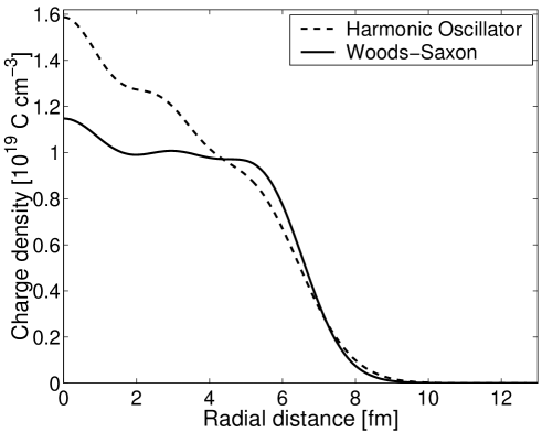
Figure 3: Charge density of the Pb nucleus derived from the harmonic oscillator model and a Wood-Saxon potential fit.

The binding energies, which also enter in the calculation of the wave functions of the outgoing protons and in the phase space factors, were taken from [33].

The current of a spinless proton could be modeled by the widely used electric Sachs form factor $G_{E}$ [34]:

$$G_{E}(Q^{2})=(1+Q^{2}/(843\,\mbox{MeV})^{2})^{-2}\,,$$ (52)

which can be expanded by the same method as the photon propagator (46). It is expected that (52) also provides a good description of the form factor of a proton inside a nucleus [3]. For the energy range considered in this paper, the contribution from magnetic scattering must not be neglected. For the calculations, we used the free nucleon current given in [6] and introduced by de Forest [35]

$$j^{\mu}_{n}=e\bar{\Psi}_{n,f}{\hat{J}}_{n}^{\mu}\Psi_{n,i}\,,$$ (53)

where

$${\hat{J}}_{n}^{\mu}(cc2)=F_{1}\gamma^{\mu}+\frac{i\kappa}{2m_{n}}\sigma^{\mu\nu}q_{\nu}F_{2},$$ (54)

and $q_{\nu}=p^{\prime}_{\nu}-p_{\nu}$ denotes here the difference between the proton four-momenta of the initial and final state, $\kappa$ the anomalous magnetic moments of the corresponding nucleon. In configuration space, the three-momenta have to be considered as gradient operators. $F_{1,2}$ are the nucleon form factors related in the usual way to the electric and magnetic Sachs form factors.

The relativistic form of the wave function for the bound protons and neutrons was constructed from the nonrelativistic wave function. Whereas the large component of the corresponding correctly normalized Dirac spinor was obtained directly from the nonrelativistic wave function, the small component was derived from the large component in a straightforward way by treating the nucleon wave function as a free Dirac plane wave. The momenta of the nucleons which were used in the current can be calculated from energy and momentum conservation. But in order to improve our model for the current, we adopted additionally an effective momentum approximation for the nucleons, where the influence of the energy-dependent optical potential on the ejected nucleons was taken into account. We found that different choices for the nucleon current do not affect significantly the ratio of the PWBA and eDWBA calculations. This is not the case for the cross section themselves. An alternative choice to the cc2 current is the cc1 current given by the operator [35]

$${\hat{J}}_{n}^{\mu}(cc1)=(F_{1}+\kappa F_{2})\gamma^{\mu}-\frac{({p^{\prime}}^{\mu}+p^{\mu})}{2m_{N}}\kappa F_{2},$$ (55)

which was also used in order to check how the ratio of the cross sections behaves for different models of the nuclear current. None of the expressions for the current (cc1,cc2) is fully satisfactory and both expressions fail to fulfill current conservation, but given the fact that we focus mainly on the electronic part of the problem, the simple choices given above provide a satisfactory description of the proton current. For the cc2 choice, integration by parts allows one in a simple way to get rid of the momentum operators acting on the nucleon wave functions.

Some critical remarks which highlight the approximations made within our single particle model are in order. Due to the fact that we are working in real space, we scaled the nucleon wave functions according to the experimental rms radius of the nucleus. This does not automatically imply that the momentum distribution of the nucleons is described very accurately. The difference between the theoretical Fermi momentum obtained in our model and the experimental value is of the order of 10%. Additionally, the choice to use an effective momentum approximation for the nucleons is an ad hoc prescription, which differs from the naive plane wave approximation for nucleons where the influence of an optical potential is neglected. In both cases, one has to accept that focusing effects of the nucleon wave functions in the nuclear region are missing and furthermore that unitarity is violated to a certain degree.

Kim et al. [6] presented calculations where plane waves and Dirac wave functions were used for the electrons, but the nucleon wave functions were calculated in both cases from a relativistic $\sigma-\omega$ model. For the kinematical situation presented in Fig. 6 in the next section, their theoretical cross sections are slightly below the experimental values, whereas our model leads to cross sections slightly above the experimental values. The advantage of our model is that we obtain a curve which shows a very similar behavior as the experimental curve, although this should not be considered as a virtue of our method. We expect that our model provides reliable results only for the ratio of cross section (were one uses plane waves or ’exact’ wave functions for the electrons), which can be used for the analysis of experimental data. We checked this assumption by varying the optical potential, the binding energies and by rescaling the wave functions within reasonable limits. The relatively large impact of such variations on the cross section is divided out for the most part in the ratio of the cross sections.

Kim et al. [36] presented also a simplified model where free plane wave functions for the ejected nucleons and harmonic wave functions for the bound nucleons were used. Adopting the same strategy in our case, we obtain nearly identical results as those presented in [36] when we scale our wave functions according to the experimental value of the nuclear Fermi momentum.

The numerical evaluation of (40) was performed by putting the nucleus on a three dimensional grid with a side length of 36 fm and using the Simpson method as a very simple but efficient integration tool. The number of necessary grid points is mainly dictated by the wave length of the oscillatory term $e^{i(\vec{k}_{i}-\vec{k}_{f}-\vec{p}_{f})}$ and was in the range of $60^{3}$ to $120^{3}$ in order to ensure an accuracy of $10^{-2}$ percent for the values of the integrals.

It is instructive to have a (classical) look a the approximate size of the different effects which lead altogether to the CC. As a specific case we choose the initial energy of the electron $\epsilon_{i}=485$ MeV, scattering angle $\theta_{e}=60^{o}$ and and energy transfer $\omega=100$ MeV. Additionaly, we take the Coulomb potential energy $V(0)$ of an electron in the center of a ²⁰⁸Pb nucleus as $-25$ MeV. The focusing then enters in the cross section as a factor $(510/485)^{2}(410/385)^{2}\sim 1.25$, i.e. it leads to an increase of the cross section of about $25$%. From the photon propagator term $\sim q^{-4}$ on the contrary we obtain a reduction by a factor of $0.80$. If we use the potential at the surface of the nucleus $-17$ MeV, the reduction factor is $0.85$. This discrepancy illustrates the importance of having an accurate description of the electron wave function. Furthermore, the form factor of the proton enters the cross section as a factor of the order of $\sim(1+Q^{2}/(843\,\mbox{MeV})^{2})^{-4}$, reducing the cross section by $6$-$9$% (for V(0)= $-17$ Mev to $-25$ MeV). Finally, the nontrivial change of the interaction which involves the detailed structure of the current via the nucleon wave functions gives an effect of several percent. All these effects described above combine to a CC which is almost zero for the present example.

3 Results

3.1 Comparison of the results to other approaches

Fig. 4 shows the ratio of the inclusive cross section for nucleon knockout with and without CC for electrons with initial energy of $\epsilon_{i}=485$ MeV and scattering angle $\Theta_{e}=60^{o}$ on ²⁰⁸Pb. Neutron knockout contributes by about 20% to the total nucleon knockout cross section in the considered kinematical region. The results obtained by Kim et al. [6] and the eikonal approximation are in good agreement, also for different kinematics as e.g. shown in Fig. 5. The result for the local effective momentum approximation (LEMA) of Kim et al., which is based on parameters that were fitted to the exact calculation, is also fairly close.

The conditions presented in Fig. 5 correspond to a similar momentum transfer, but large scattering angle $\Theta_{e}=143^{o}$ and incident energy $310$ MeV. The initial electron energy is smaller, and the effect of CC is more pronounced. CC lead to a sizeable modification in the longitudinal and transverse responses that can be extracted from the data via Rosenbluth plots. The linearity of the Rosenbluth plots served also as an independent check for the validity of our plane wave calculations.

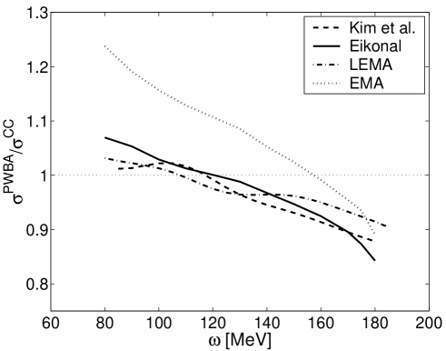
Figure 4: Comparison of the Coulomb corrections for different approaches. The dotted curve shows the ratio $\sigma_{PWBA}/\sigma_{EMA}$ according to the model used in this paper.

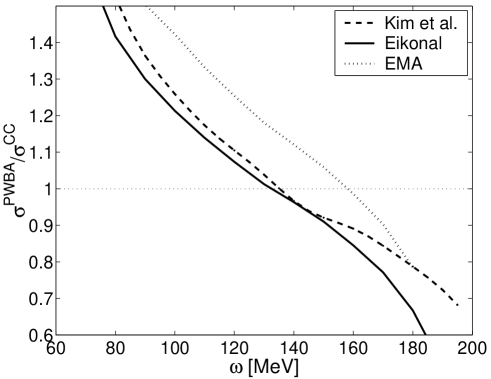
Figure 5: $\sigma_{{}_{PWBA}}/\sigma_{{}_{CC}}$ for $\epsilon_{i}=310$ MeV and $\Theta_{e}=143^{o}$. Dotted curve: $\sigma_{PWBA}/\sigma_{EMA}$ as in Fig. 4.

The calculations clearly indicate that the effective momentum approximation, which leads to admissible results for light nuclei where the CC are relatively small, is useless for highly charged nuclei. The curve in Fig. 5 was calculated by choosing a $\Delta k=25$ MeV/c according to Eq. (2). Taking smaller values for $\Delta k$ corresponding to the electrostatic potential at the surface of the nucleus does not change the situation significantly.

It is important to take into account the final state interaction of the proton by an energy-dependent optical potential. For protons with energies above $100$ MeV, the potential is becoming increasingly repulsive. Calculations for $\omega>180$ MeV in our single particle shell model are not applicable, since pion production is not included in our calculations, and correlation effects are becoming increasingly important for large $\omega$. Results for $\omega<80$ MeV may also become dubious due to the large distortion of the outgoing proton wave function by the final state interaction, but the simple approximation given in this work allows for a good estimation of CC in a relatively wide range of energies.

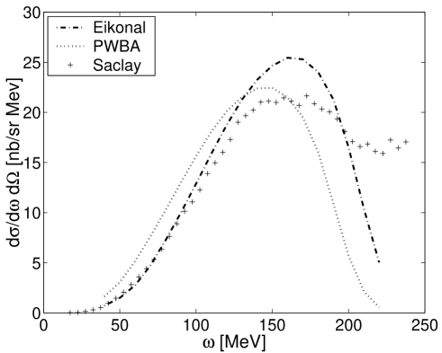
Figure 6: Comparison of theoretical cross sections obtained in PWBA and eikonal approximation to experimental Saclay data ($\epsilon_{i}=310$ MeV and $\Theta_{e}=143^{o})$.

It is a well-known phenomenon that plane wave calculations have a tendency to overestimate cross sections in the region of low electron energy loss, whereas cross sections are underestimated in the high energy loss region. The reason for this is the fact that the use of plane waves for the ejected nucleons is clearly a rough approximation, and the generally used single particle model does not contain contributions arising from correlations and meson-exchange currents. Inelastic scattering from the nucleons, i.e. excitation of the delta resonance, is also absent.

Nevertheless, the agreement between experimental data taken at Saclay [37] and our eikonal corrected calculations is quite satisfactory, as displayed in Fig. 6 in order to give a typical example. Like in the case $\Theta_{e}=60^{o}$, one observes that the CC become very large for high energy transfer $\omega\simeq 180$ MeV. This result should be handled with care, since the calculated cross sections become small in this energy region. The electroproduction of the delta resonance will have to be included to more reliably estimate the CC at very large energy loss.

Overall, we find that the eikonal approach gives results that are very close to the results from exact calculations. This approach can thus be used in practical applications where one greatly benefits from the much lower calculational effort involved in the eikonal description. At the same time, our calculation shows again that the often-used effective momentum approximation is inadequate for a quantitative treatment of Coulomb corrections.

3.2 Study of the Coulomb distortion by comparing quasielastic electron and positron scattering

The comparison of experimentally determined quasielastic cross sections induced with electrons and with positrons represent an ideal test for any theoretical approach to quantitatively describe Coulomb distortions. Here we consider a recent experiment by Guèye et al. [38] which was used to give an experimental proof of the validity of the EMA for inclusive quasielastic electron scattering. The experiment by Guèye et al. compared quasielastic scattering of electrons on ²⁰⁸Pb with quasielastic scattering of positrons at the same kinematics.

Figure 7: Scaling function $F(y)$ obtained from cross sections measured by Zghiche et al. on ²⁰⁸Pb at an electron scattering angle of 60 degrees and initial electron energy $E$. $F(y)$ is obtained from the cross sections by dividing out the Mott cross section and the $q$-dependence of the nucleon form factors (both smooth functions of incident energy).

With the assumption that the EMA is a valid approach the authors interpolate the experimental $e^{-}$–data linearly to the effective energy of the $e^{+}$–data, $E_{e^{+}}=E_{e^{-}}-2V_{c}$ with the Coulomb potential $V_{c}$ and the relative normalization as fit parameters. They find for $V_{c}$ a value close to the surface and a normalization factor which is compatible with the experimental uncertainties. For the interpolation the large body of inclusive quasielastic data on ²⁰⁸Pb measured by Zghiche et al. [37] is used. The authors conclude that a modified EMA with a $V_{c}(r)=18.7$ MeV close to the surface is a valid approach to correct cross section data.

However, this conclusion is highly questionable when the quality of the data by Zghiche et al. is studied. The peculiar behavior of the data is shown in Fig. 7, where the scaling function $F(y)$ (essentially the cross section but with the $q$-dependence of the nucleon form factor and the kinematical broadening of the quasielastic peak removed) is shown (see [3] for detailed definitions). Although the electron energies progress in regular steps between the various data sets, the scaling functions $F(y)$ display a curious behavior. The peak values for $F(y)$ for two consecutive energies coincide and jump for the following to a significantly lower value. In Fig. 10 in [37], the staircase-like behavior of the data is not visible, since cross sections are plotted, which depend strongly on the initial electron energy $\epsilon_{i}^{e}$. Additionally, the cross sections for $e_{i}^{e}=420$ MeV and $e_{i}^{e}=600$ MeV are missing there. But the staircase-like behavior has a detrimental effect upon the interpolation of the electron data as shown by Guèye et al. Also, the $e^{+}$ and $e^{-}$ data of Guèye et al. have been $e^{+}$ beam emittance corrected and normalized to the $e^{-}$ data shown in Fig. 7, hereby further affected by the staircase behavior. We therefore cannot consider the experiment as a proof of the validity of the EMA.

We performed eikonal and effective momentum calculations for quasielastic electron (e) and positron (p) scattering on ²⁰⁸Pb for a kinematics also used in the experiment of Guèye et al., i.e. for initial energy $\epsilon_{i}^{e}=\epsilon_{i}^{p}=420$ MeV and scattering angle $\Theta_{e}=\Theta_{p}=60^{o}$. The calculations for the positrons were performed in a strictly analogous way as in the case of electrons. Using an effective surface value of $17$ MeV for the repulsive (attractive) Coulomb potential in the case of the positron (electron) EMA calculation, it turns out that the eikonal approximation and the EMA are clearly incompatible. The observed discrepancy can be explained by the assumption that the EMA underestimates the defocusing of the positron waves and the focusing of the electron wave in the nuclear volume.

For the sake of completeness, we also show in Fig. 10 experimental cross sections for positrons derived from the total response function given in [38], which are in satisfactory agreement with the theoretical values shown in Fig. 9. As explained before, the difference between experimental data and the theoretical cross sections results from the simple nuclear model employed (lack of high momenta in the corresponding spectral functions and the absence of delta excitations and meson exchange current contributions).

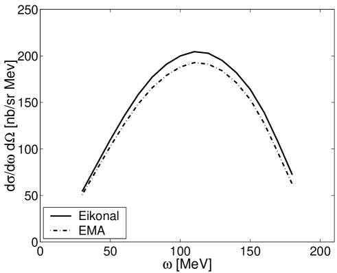
Figure 8: Theoretical cross sections for inclusive quasielastic electron scattering off ²⁰⁸Pb for initial electron energy $\epsilon_{i}^{e}=420$ MeV and scattering angle $\Theta_{e}=60^{o}$.

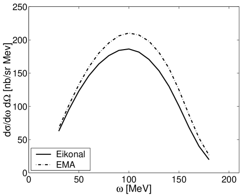
Figure 9: Theoretical cross sections for inclusive quasielastic positron scattering off ${}^{208}\mbox{Pb}$ for initial positron energy $\epsilon_{i}^{p}=420$ MeV and scattering angle $\Theta_{p}=60^{o}$.

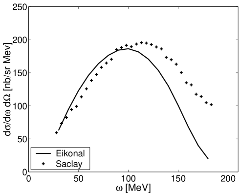
Figure 10: Experimental positron cross sections derived from the total response function given by Guèye et al., compared to the theoretical values shown in Fig. 9 obtained from the single particle model.

4 Conclusions

In the present paper we have investigated the role of the Coulomb distortion in quasielastic electron nucleus scattering. A reliable treatment of this distortion is needed in particular for a determination of the longitudinal response function and for an extrapolation of nuclear responses to infinite nuclear matter.

We have developed an approximate description –the eikonal approximation– that is more transparent and numerically easier to deal with than the exact treatments (solution of the full Dirac equation) previously employed [6, 7, 8]. At the same time, the eikonal approximation is much more realistic than the effective momentum approximation often employed in the absence of results from exact calculations.

We find that the eikonal results for the Coulomb distortion are very close to the results of exact calculations. We also find that the effective description of the Coulomb distortion gives a rather poor description for high values of the nuclear charge $Z$.

Appendix

The potential energy of the electron according to Eq. (23) can be decomposed into three parts $V(r)=V_{1}(r)+V_{2}(r)+V_{3}(r)$, where

$$V_{1}(r)=-\frac{\alpha Z}{(r^{2}+R^{2})^{1/2}},\quad V_{2}(r)=-\frac{\alpha ZR^{2}}{2(r^{2}+R^{2})^{3/2}},$$

$$V_{3}(r)=-\frac{24\alpha ZR^{2}R^{\prime}r^{4}}{25\pi(r^{2}+R^{\prime 2})^{4}}.$$ (56)

The regularized eikonal phase $\chi_{1}$ generated by $V_{1}$ is given above by Eq. (26). Since $V_{2,3}$ decrease faster than $r^{-1}$ for large $r$, their corresponding contributions to the total eikonal phase for a particle incident parallel to the z-axis with impact parameter $b$

$$\chi_{2,3}(\vec{r})=\chi_{2,3}(b,z)=-\int\limits_{-\infty}^{z}dz^{\prime}\,V_{2,3}(r^{\prime}),\quad r^{\prime 2}=b^{2}+z^{\prime 2}$$ (57)

need not be regularized. The integrals in (57) are given by

$$\chi_{2}=\frac{\alpha Z}{2}\frac{R^{2}(z+(r^{2}+R^{2})^{1/2})}{(b^{2}+R^{2})(r^{2}+R^{2})^{1/2}},$$ (58)

$$\frac{25\pi}{\alpha ZR^{2}R^{\prime}}\chi_{3}=\Biggl{(}\frac{15}{2}\frac{b^{4}}{b^{\prime 7}}+\frac{3b^{2}}{b^{\prime 5}}+\frac{3}{2b^{\prime 3}}\Biggr{)}\arctan\Biggl{(}\frac{z}{b^{\prime}}\Biggr{)}-\frac{7z}{(r^{2}+R^{\prime 2})^{2}}$$

$$+\frac{4b^{4}z}{b^{\prime 2}(r^{2}+R^{\prime 2})^{3}}+\frac{5b^{4}z}{b^{\prime 4}(r^{2}+R^{\prime 2})^{2}}+\frac{15b^{4}z}{2b^{\prime 6}(r^{2}+R^{\prime 2})}-\frac{8b^{2}z}{(r^{2}+R^{\prime 2})^{3}}$$

$$+\frac{2b^{2}z}{b^{\prime 2}(r^{2}+R^{\prime 2})^{2}}+\frac{3b^{2}z}{b^{\prime 4}(r^{2}+R^{\prime 2})}+\frac{4b^{\prime 2}z}{(r^{2}+R^{\prime 2})^{3}}+\frac{3z}{2b^{\prime 2}(r^{2}+R^{\prime 2})}$$

$$+\frac{3\pi}{4}\frac{5b^{4}+2b^{\prime 2}b^{2}+b^{\prime 4}}{b^{\prime 7}},$$ (59)

where $r^{2}=b^{2}+z^{2}$ and $b^{\prime}=\sqrt{b^{2}+R^{\prime 2}}$. The coordinate independent definitions of the parameters $z$, $b$, and $b^{\prime}$ are $z=(\vec{k}_{i}\vec{r})/k_{i}$ and $b^{2}=r^{2}-z^{2}$, $b^{\prime}=\sqrt{b^{2}+R^{\prime 2}}$, where $\vec{k}_{i}$ is the momentum of the incident electron. The eikonal phase of the wave function of the outgoing electron with momentum $\vec{k}_{f}$, which must be added to the eikonal phase of the incoming electron in the matrix element of the calculated process, can be obtained directly from the expressions above by replacing $z=-(\vec{k}_{f}\vec{r})/k_{f}$ and using again the definitions $b^{2}=r^{2}-z^{2}$, $b^{\prime}=\sqrt{b^{2}+R^{\prime 2}}$.

References

- [1] R.R. Whitney, I. Sick, J.R. Ficenec, R.D. Kephart, W.P. Trower, Phys. Rev. C9, 2230-2235 (1974).
- [2] O. Benhar, A. Fabrocini, S. Fantoni, I. Sick, Phys. Lett. B343, 47-52 (1995).
- [3] J. Jourdan, Nucl. Phys. A603, 117-160 (1996).
- [4] D. Day, J.S. McCarthy, T.W. Donnelly, I. Sick, Ann. Rev. Nucl. Part. Sci. 40, 357-410 (1990).
- [5] D.B. Day, J.S. McCarthy, Z.E. Meziani, R.C. Minehart, R.M. Sealock, S.T. Thornton, J. Jourdan, I. Sick, B.W. Filippone R.D. McKeown, R.G. Milner, D.H. Potterveld, Z. Szalata, Phys. Rev. C40, 1011-1024 (1989).
- [6] K.S. Kim, L.E. Wright, and Y. Jin, Phys. Rev. C 54, 2515-2524 (1996).
- [7] J.M. Udias, J.R. Vignote, E. Moya de Guerra, A. Escuderos, J.A. Caballero, Recent developments in relativistic models for exclusive A(e,e’p)B reactions, Workshop on ”e-m induced Two-Hadron Emission”, Lund, June 13-16, 2001.
- [8] J.M. Udias, P. Sarriguren, E. Moya de Guerra, E. Garrido, J.A. Caballero, Phys. Rev. C48, 2731-2739 (1993).
- [9] D.R. Yennie, F.L. Boos, and D.G. Ravenhall, Phys. Rev. 137, no. 4B, 882-903 (1965).
- [10] C. Giusti, F.D. Pacati, Nucl. Phys. A473, 717-735 (1987).
- [11] C. Giusti, F.D. Pacati, Nucl. Phys. A485, 461-480 (1988).
- [12] D. R. Yennie, D. G. Ravenhall, R. N. Wilson, Phys. Rev. 95, 500-512 (1954).
- [13] F. Lenz, Ph.D. thesis, Freiburg, Germany, 1971.
- [14] J. Knoll, Nucl. Phys. A223, 462-476 (1974).
- [15] M. Traini, S. Turck-Chieze, A. Zghiche, Phys. Rev. C38, 2799-2812 (1988).
- [16] M. Traini, M. Covi, Nuovo Cim. A108, 723-736 (1995).
- [17] K. S. Kim, L. E. Wright, Y. Jin, D. W. Kosik, Phys. Rev. C54, 2515-2524 (1996).
- [18] F. Lenz, R. Rosenfelder, Nucl. Phys. A176, 513-525 (1971).
- [19] R. Rosenfelder, Annals Phys. 128, 188-240 (1980).
- [20] M. Levy, J. Sucher, Phys. Rev. 186, 1656-1670 (1969).
- [21] R.L. Sugar, R. Blankenbecler, Phys. Rev. 183, 1387-1396 (1969).
- [22] S.J. Wallace, Annals Phys. 78, 190-257 (1973).
- [23] S.J. Wallace, J.A. McNeil, Phys. Rev. D16, 3565-3580 (1977).
- [24] H. Abarbanel, C. Itzykson, Phys. Rev. Lett. 23, 53-56 (1969).
- [25] Y. Jin, D.S. Onley, L.E. Wright, Phys. Rec. C45, 1311-1320 (1992).
- [26] Y. Jin, D.S. Onley, L.E. Wright, Phys. Rev. C50, 168-176 (1994).
- [27] J. Jourdan, Workshop on Electron-Nucleus Scattering, eds. O. Benhar, A. Fabrocini, Edizioni ETS, Pisa, p. 319 (1997).
- [28] A. Baker, Phys. Rev. B134, 240-251 (1964).
- [29] R.J. Glauber, Lecture Notes in Theoretical Physics, vol. I, Interscience, New York (1959).
- [30] A.J. Koning, J.P. Delaroche, Nucl. Phys. A713, 231-310 (2003).
- [31] Y. Jin, D.S. Onley, L.E. Wright, Phys. Rev. C45, 1333-1338 (1992).
- [32] B. C. Clark, L. J. Kerr, S. Hama, Phys. Rev. C67, 054605 (2003).
- [33] M. van Batenburg, Deeply-bound protons in 208Pb, Ph. D. thesis, University of Utrecht, Netherlands (2001).
- [34] G. Höhler, E. Pietarinen, I. Sabba-Stevanescu, F. Borkowski, G.G. Simon, V.H. Walter, R.D. Wendling, Nucl. Phys. B144, 505-534 (1976).
- [35] T. de Forest, Jr., Nucl. Phys. A392, 232-248 (1983).
- [36] K.S. Kim, L.E. Wright, D.A. Resler, Phys. Rev. C64, 044607 (2001).
- [37] A. Zghiche, J.F. Daniel, M. Bernheim, M. Brussel, G.P. Capitani, E. de Sanctis, S. Frullani, F. Garibaldi, A. Gerard, J.M. Le Goff, A. Magnon, C. Marchand, Z. E. Meziani, J. Morgenstern, J. Picard, D. Reffay-Pikeroen, M. Traini, S. Turck-Chieze, P. Vernin, Nucl. Phys. A572, 513-559 (1994).
- [38] P. Gueye, M. Bernheim, J.F. Danel, L. Lakehal-Ayat, J.M. LeGoff, A. Magnon, C. Marchand, J. Morgenstern, J. Marroncle, P. Vernin, A. Zghiche-Lakehal-Ayat, V. Breton, S. Frullani, F. Garibaldi, F. Ghio, M. Iodica, D.B. Isabelle, Z.-E. Meziani, E. Offermann, M. Traini, Phys. Rev. C60, 044308 (1999).