Origin of chaos in the spherical nuclear shell model: role of symmetries

Abstract

To elucidate the mechanism by which chaos is generated in the shell model, we compare three random–matrix ensembles: the Gaussian orthogonal ensemble, French’s two–body embedded ensemble, and the two–body random ensemble (TBRE) of the shell model. Of these, the last two take account of the two–body nature of the residual interaction, and only the last, of the existence of conserved quantum numbers like spin, isospin, and parity. While the number of independent random variables decreases drastically as we follow this sequence, the complexity of the (fixed) matrices which support the random variables, increases even more. In that sense we can say that in the TBRE, chaos is largely due to the existence of (an incomplete set of) symmetries.

and

1 Introduction and Motivation

The analysis of nuclear spectra has produced ample evidence for chaotic motion. Indeed, near neutron threshold, the spectra of medium–weight and heavy nuclei display fluctuations which agree with those of random matrices drawn from the Gaussian orthogonal ensemble (GOE) [1]. Similar agreement has been found for nuclei in the $sd$–shell (both in experimental data [2] and in shell–model calculations [3]), and in the ground–state domain of heavier nuclei [4], although here there exists strong evidence, too, for regular motion as predicted by the shell model and the collective models. Calculations in Ce [5] have produced similar evidence for chaotic motion in atoms. Thus, chaos appears to be an ubiquitous feature of interacting many–body systems. What is the origin of this behavior? In the present paper, we address aspects of this question.

We do so using the nuclear shell model, a theory with a mean field and a residual two–body effective interaction $V$. (We do not include three–body forces, although there is evidence [6] that these may be needed to attain quantitative agreement with data. It will be seen that qualitatively, our arguments would not change with the inclusion of such forces.) In many nuclei, the mean field is (nearly) spherically symmetric. Thus, single–particle motion is largely regular. Chaos in nuclei seems a generic property and, hence, must be due to $V$. We focus attention entirely upon the effects of $V$. Therefore, we assume that we deal with a single major shell in which the single–particle states are completely degenerate and in which there is a fixed number of valence nucleons. (A lack of complete degeneracy would reduce the mixing of states due to $V$ and, thus, drive the system towards regular motion). Generic results are expected to be independent of the details of $V$. Therefore, we assume that the two–body matrix elements (TBME) of $V$ are uncorrelated Gaussian–distributed random variables with zero mean value and unit variance. Our results then apply to almost all two–body interactions with the exception of a set of measure zero. (The integration measure is the volume element in the parameter space of the TBME.) The resulting random–matrix model is commonly referred to as the two–body random ensemble (TBRE) [7, 8]. We ask: How does $V$ produce chaos in the framework of the TBRE?

The two–body interaction $V$ has two characteristic features. (i) It connects pairs of nucleons. (ii) It possesses symmetries: it conserves spin, isospin, and parity. We wish to elucidate the role of both features in producing chaos in nuclei.

The relevance of the first feature is brought out by comparing the TBRE with the GOE. We recall that in the latter, the matrix elements of the Hamiltonian couple every state in Hilbert space to every other such state. These matrix elements are assumed to be uncorrelated random variables. In the context of many–body theory, such independent couplings between all pairs of states can be realized only in terms of a many–body interaction the rank of which equals the number of valence particles. Put differently, with $N$ the dimension of the Hamiltonian matrix, the number of independent random variables in the GOE is $N(N+1)/2$ and, for $N\to\infty$, grows much faster than $N$. Thus, it is intuitively clear that the GOE Hamiltonian will produce a thorough mixing of the basis states which is tantamount to chaos. In contradistinction, the number of independent two–body matrix elements in a single shell with half–integer spin $j$ is only $j+1/2$ while the number of many–body states with fixed total spin $J$ grows with $j$ like $j^{m-3}$ where $m$ is the number of valence particles. (The simple estimates leading to these statements are given in the Appendix. The statements apply for $j\gg m\gg 1$, and $J\ll m$). Thus, in the TBRE the number of independent random variables is much smaller than the dimension of typical matrix spaces, and it is a non–trivial fact that $V$ produces as much mixing of the basis states as the GOE Hamiltonian. We wish to elucidate the mechanism which is responsible for this mixing.

As for the second feature (the role of symmetries), we compare the TBRE with another random–matrix model which lacks the symmetries of the TBRE but likewise assumes a random two–body interaction. This is the embedded two–body ensemble of Gaussian orthogonal random matrices (EGOE(2)) [9]. (For a recent review we refer the reader to Ref. [10]). In this model, $m$ fermions are distributed over $l>m$ degenerate single–particle states. Hilbert space is spanned by the resulting $N={l\choose m}$ Slater determinants. The two–body interaction connects only those Slater determinants which differ in the occupation numbers of not more than two single–particle states. Therefore, the representation of the two–body interaction in the Hilbert space of Slater determinants yields a sparse matrix (most non–diagonal matrix elements vanish). This model does not respect the symmetries of the shell model. Neither the single–particle states nor the two–body interaction carry any quantum numbers. Obviously, the model is very different from the GOE. It is likewise very different from the TBRE. In the latter, the single–particle states do carry spin, isospin, and parity quantum numbers, and $V$ conserves these symmetries. Total Hilbert space decays into orthogonal subspaces carrying these same quantum numbers. Each subspace is spanned by states which are linear combinations of (many) Slater determinants. As a result, the matrix representation of $V$ in any such subspace becomes fairly dense, even though it remains true that $V$ connects only Slater determinants which differ in the occupation numbers of not more than two single–particle states.

In comparing the EGOE(2) and the TBRE, one may consider several options. (i) One might use the fixed Hilbert space of all many–body states that exist within a given major shell, with all possible quantum numbers for total spin, parity, and isospin. These states are coupled either via a symmetry–preserving random interaction (this is the TBRE; here the Hamiltonian has block–diagonal structure), or via a symmetry–breaking random interaction (this is the EGOE(2)). One might compare the spectral statistics of the eigenvalues and the mixing of the eigenfunctions in both models. At this point in time, such a comparison is impractical because of the huge dimension of the matrices involved for the EGOE(2). (ii) One might use a Hilbert space of many–body states with fixed values for total spin, parity and isospin. These states are coupled again either via a symmetry–preserving random interaction (this is the TBRE within the subspace of many–body states with fixed quantum numbers) or, in the case of a symmetry–breaking interaction, via effective interactions that take into account the coupling to many–body states with different quantum numbers. Here the construction of the effective interaction poses severe difficulties and is practically impossible for realistic cases. Both options (i) and (ii) ask questions relating to the physical role of conserved quantum numbers in the shell model. Even if these options were open, we would probably not have used them. The aim of this paper is different. We wish to elucidate the mechanisms which are operative in different random–matrix models (GOE, EGOE(2), TBRE) in generating chaos. This is why we have followed option (iii): The role of symmetries can also be displayed by comparing the structure of the Hamiltonian matrices which are typical for the TBRE and the EGOE(2), in both cases for Hilbert spaces of large dimensions. This option does not require the diagonalization of huge matrices or the difficult construction of effective interactions. It dodges the issue of the physical role of symmetry in shell–model calculations and focusses instead upon the structural aspects of the matrices involved in the two approaches.

In Section 2 we elucidate the structural features of the EGOE(2). In Section 3 we then turn to a corresponding analysis for the TBRE in the case of a single $j$–shell, and of the $sd$–shell. For both models we aim at displaying those structural elements which are absent in the GOE and which are essential for producing a thorough mixing of the basis states in Hilbert space and, thus, chaos, in spite of a strongly reduced number of independent random variables. The comparison between the EGOE(2) and the TBRE will then display the role of symmetries in the TBRE. (This aspect of the TBRE has been coined “geometric chaoticity” by Zelevinsky et al. [3]. To the best of our knowledge, however, the actual role of symmetries in the TBRE has never been investigated.) We are led to the conclusion, that symmetries are a vital element of the TBRE and, in this sense, instrumental in producing chaos in nuclei.

We are aware of a huge body of literature addressing issues closely related to our theme. Some of these are reviewed in Refs. [3, 10, 11]. As mentioned above, there is ample evidence for chaos in nuclear shell–model calculations in the $sd$–shell and beyond. Likewise, there is evidence for chaos in the EGOE(2), at least in the center of the spectrum. Even deviations from complete chaos have been understood since a long time. As early as 1979, it was, f.i., shown [12] that the non–degeneracy of the single–particle states in the $sd$–shell prevents a complete mixing of all the states of given total spin and causes the partial width amplitudes (given as projections of the eigenstates of the shell–model Hamiltonian onto a fixed vector in Hilbert space) to deviate from the Porter–Thomas distribution predicted by the GOE. We are not concerned with adding to this impressive body of evidence. We take it for granted that chaos exists in the shell model and in the EGOE(2). Rather, we wish to understand the structural aspects of the TBRE and of the EGOE which produce chaos.

We believe that our investigation offers novel insights into the origin of chaos in nuclei in the following two respects: (i) We demonstrate that chaos is generic and ubiquitous both in a single $j$–shell and in the $sd$–shell. To the best of our knowledge, previous arguments have always relied upon numerical results based upon a specific choice of the two–body interaction. In contradistinction, we use generic aspects of the TBRE to show that we must always expect strong mixing of the basis states. (ii) We exhibit the role played by symmetries in the TBRE for the generation of chaos by comparing this ensemble with the EGOE(2), and with the GOE. We are not aware of any previous work on this topic.

Our emphasis on the role of symmetry in generating chaos may be surprising. In fact, the existence of a complete set of quantum numbers (usually connected to symmetries of the Hamiltonian) is equivalent to integrability and, thus, diametrically opposed to chaos. The case of nuclei (and, for that matter, of atoms) is different. The symmetries that dominate nuclei (invariance under rotation, mirror reflection, and proton–neutron exchange) are incomplete (they do not form a complete set of integrals of the motion). Taking account of these symmetries, we can write the Hamiltonian in block–diagonal form. Chaotic motion does seem to exist in every such block. Therefore, it is meaningful to ask: In which way is the origin of chaos influenced by the presence such an incomplete set of quantum numbers? It is this question which we answer by comparing the TBRE with the EGOE(2) and the GOE.

2 Absence of Symmetries

In this Section, we analyse the EGOE(2) and then compare it with the GOE. In the absence of symmetries, the appropriate random two–body interaction model is the EGOE(2). The EGOE(2) is often used to model stochastic aspects of realistic systems like small metallic grains or quantum dots. This is justified since in those systems the single–particle wave functions themselves are chaotic, and the resulting two–body matrix elements reflect this property and transport the information of the underlying one–body chaos into the many–body system. Several numerical studies for matrix dimensions up to a few thousand or so have shown that the EGOE(2) exhibits GOE statistics in the center of the spectrum. For infinite matrix dimensions, the situation is less clear. Evidence from previous work on the EGOE(2) [13, 11] suggests that the level statistics is Poissonian. However, no firm conclusion has yet been reached [14]. Here, we supplement the previous analysis by a different approach and focus on the matrix structure. In the EGOE(2), the random variables are the $a={l\choose 2}[{l\choose 2}+1]/2$ independent two–body matrix elements $V_{\alpha},\alpha=1,\ldots,a$. A Hamiltonian drawn from the EGOE(2) has matrix elements

$$H_{\mu\nu}=\sum_{\alpha=1}^{a}V_{\alpha}D_{\mu\nu}(\alpha)\ ,$$ (1)

where the matrices $D_{\mu\nu}(\alpha)$ transport the information contained in the two–body matrix elements $V_{\alpha}$ into the $N$–dimensional Hilbert space spanned by Slater determinants labeled $\mu$ or $\nu$.

The matrices $D$ play a central role in the understanding of the EGOE(2). Indeed, these matrices are the structural elements of this ensemble, while the $V_{\alpha}$’s are just a set of random variables that change from realization to realization. Pictorially speaking, the matrices $D$ form the scaffolding which supports the random variables $V_{\alpha}$. The properties of the EGOE(2) (averages, higher moments and correlation functions) of both the Hamiltonian and the Green’s functions are completely determined by the matrices $D$.

The ensemble average of the Hamiltonian is obviously zero. The second moment is

$$\overline{(H_{\mu\nu})^{2}}=\sum_{\alpha}(D_{\mu\nu}(\alpha))^{2}\ .$$ (2)

The properties of the matrices $D_{\mu\nu}$ are obtained by counting. Let $\mu$ and $\nu$ differ in the occupation numbers of $f$ single–particle states. (a) If $f\geq 3$, then $\sum_{\alpha}(D_{\mu\nu}(\alpha))^{2}=0$. (b) If $f=2$, then $\sum_{\alpha}(D_{\mu\nu}(\alpha))^{2}=1$. (c) If $f=1$, then $\sum_{\alpha}(D_{\mu\nu}(\alpha))^{2}=(m-1)$. (d) If $f=0$ or $\mu=\nu$, then $\sum_{\alpha}(D_{\mu\mu}(\alpha))^{2}={m\choose 2}$. For the number of times each of these alternatives is realized, we find (a) $\sum_{j\geq 3}N{m\choose j}{l-m\choose j}$, (b) $N{m\choose 2}{l-m\choose 2}$, (c) $Nm(l-m)$, and (d) $N$. The number of zero matrix elements dominates (it is close to $N^{2}$). The number of unit values comes next and is approximately $(1/4)Nm^{2}(l-m)^{2}$. The number of values $(m-1)$ is $Nm(l-m)$. The number of values ${m\choose 2}$ is trivially equal to $N$, the dimension of the matrix and the number of diagonal elements. The correlators $\sum_{\alpha}D_{\mu\nu}(\alpha)D_{\rho\sigma}(\alpha)$ can also be worked out easily but are not given here. They do not all vanish. Therefore, the random variables $V_{\alpha}D_{\mu\nu}(\alpha)$ are not independent. This reflects the fact that the same matrix element of the two–body interaction may couple different pairs of Slater determinants.

The individual matrices $D_{\mu\nu}(\alpha)$ have a very simple structure and barely mix many-body states. Let the TBME corresponding to index $\alpha$ change the occupation of $f$ particles. For $f=0$ the matrix $D_{\mu\nu}(\alpha)$ is diagonal. For $f=1,2$ the matrix $D_{\mu\nu}(\alpha)$ can be ordered to have ${l-2-f\choose m-2}$ block matrices of dimension two and is zero otherwise. This shows that individual matrices $D_{\mu\nu}(\alpha)$ cannot generate mixing and chaos.

We consider the limit of large matrix dimension $N$, attained by taking the limit $l\to\infty$. This can be done in two ways: (i) by keeping the ratio $m/l$ fixed; (ii) by keeping $m$ fixed. (i) The ratio of the number of non–diagonal elements with variance unity to the total number of matrix elements is $(1/4)m^{2}(l-m)^{2}/N$. This ratio tends to zero as $l\to\infty$. The same ratio calculated for the non–diagonal elements with variance $(m-1)$ vanishes even faster. The correlators of the diagonal elements are $\sum_{\alpha}D_{\mu\mu}(\alpha)D_{\nu\nu}(\alpha)={k\choose 2}$ where $k$ is the number of single–particle states that are occupied in both $\mu$ and $\nu$. The correlation is maximal for $k=m-1$ and vanishes for $k=0$ and $k=1$. For fixed $\mu$ and $k$, the number of states $\nu$ for which the occupation of $k$ single–particle states is the same as in $\mu$ is ${l-m\choose m-k}{m\choose k}$. For $k=m-1$, this yields $m(l-m)$ and for $k=1$, we find $m{l-m\choose m-1}$. The ratio of both expressions to $N$ vanishes exponentially fast as $l\to\infty$. Thus, the matrices approach diagonal form with uncorrelated diagonal elements that all have the same variance. This is suggestive of the Poissonian distribution. (ii) The ratio of the number of non–diagonal elements with variance unity to the total number of matrix elements is $(1/4)m^{2}l^{2}/N$ and vanishes exponentially fast. The same holds true a fortiori for the elements with variance $m-1$. Again, the correlators of the diagonal elements are given by ${k\choose 2}$, and the number of states which correlate to a given one with this correlator is ${l-m\choose m-k}{m\choose k}$. The ratio of this value to $N$ vanishes as a power of $l$. Again, this is suggestive of the Poissonian distribution. We note, however, that sparseness of a random matrix is no guarantee for Poissonian statistics. Indeed, Fyodorov and Mirlin [15] have shown that sparse random matrices with ${\it uncorrelated}$ non–vanishing matrix elements that have a frequency $p/N$ and no preference for large diagonal elements may have either Poissonian or GOE statistics, depending on the value of $p$. While these results are quite suggestive, the question about spectral fluctuations of the EGOE(2) in the limit of large matrix dimension remains open.

We apply these considerations to the half–filled $sd$-shell (disregarding, of course, all conserved quantum numbers). The number of single–particle states is $l=24$; the number of nucleons is $m=12$. The number of independent TBME is $\approx 3.8\times 10^{4}$. The corresponding matrices of the embedded ensemble have dimension $N\approx 2.7\times 10^{6}$. The variance of the diagonal elements is $66$. The fraction of non–diagonal elements with variance unity is approximately $1.9\times 10^{-3}$, that of those with variance $m-1=11$ is approximately $5.3\times 10^{-5}$. The Hamiltonian matrices of the EGOE(2) are thus characterized by their sparsity, strong diagonal structure, and a relatively large number of independent TBME.

This structure is very different indeed from that of the GOE. In analogy to Eq. (1), the matrix elements of the GOE Hamiltonian can be written in the form

$$H^{\rm GOE}_{\mu\nu}=\sum_{j<l=1}^{N}V_{jl}D^{\rm GOE}_{\mu\nu}(j,l)\ .$$ (3)

The random variables $V_{jl}$ are defined for $1\leq j<l\leq N$ where $N$ is the dimension of $H^{\rm GOE}$ and are uncorrelated Gaussian–distributed random variables with zero mean and a common second moment. The matrices $D^{\rm GOE}$ again determine the structure of the ensemble and are given by

$$D^{\rm GOE}_{\mu\nu}(j,l)=\delta_{j\mu}\delta_{l\nu}+\delta_{j\nu}\delta_{l\mu}\ .$$ (4)

Each such matrix is symmetric and has only one non–vanishing matrix element above or in the main diagonal. Again, all ensemble averages of the GOE are determined by the matrices $D^{\rm GOE}$. In view of the extreme simplicity of these matrices, one usually does not write the GOE in the form of Eq. (3). This form is, however, useful for purposes of comparison. We observe that in the GOE, the number of independent random variables and, thus, of matrices $D^{\rm GOE}$ is as large as is consistent with the basic symmetry (invariance under time reversal) of the ensemble. In the EGOE(2) and for matrices of the same dimension $N$, the number of independent random variables and, thus, of matrices $D$ is strongly reduced. This strong reduction is accompanied by a strong increase in the number of non–vanishing matrix elements of each of the matrices $D$. Although sparse, the matrices $D$ are much less so than their GOE counterparts.

3 Presence of symmetries

In this section we consider the TBRE, both for a single $j$–shell and for the $sd$–shell. We first investigate the TBRE for the case of a single $j$–shell. This is the simplest case and already exhibits the major difference to the EGOE. Then we consider the more realistic (and more complex) case of the $sd$–shell where we encounter several sub–shells and also have to include isospin in our analysis.

We consider $m$ fermions in a single $j$–shell. (Later, we will consider the example $m=6$ and $j=19/2$). There are $a=j+1/2$ TBME as two identical particles can have spins $s=0,2,4,\ldots,(j-1)/2$. The corresponding spin–conserving two–body matrix elements are denoted by $V_{\alpha}$, with $\alpha=1,\ldots,a$. The matrix elements of the $j$-shell Hamiltonian in the space of many–body states with total spin $J$ and projection $J_{z}=0$ are

$$H_{\mu\nu}^{J}=\sum_{\alpha=1}^{a}V_{\alpha}C_{\mu\nu}^{J}(\alpha)\ .$$ (5)

Again, the matrices $C_{\mu\nu}^{J}(\alpha)$ transport the information about the TBME $V_{\alpha}$ into the space of the many–body states. With the $V_{\alpha}$ considered as uncorrelated Gaussian–distributed random variables with zero mean value and a common second moment, all properties of the TBRE (mean values, higher moments and correlation functions of both Hamiltonian and Green’s functions) are again completely determined by the matrices $C^{J}$, in full analogy to the cases of the GOE and of the EGOE(2). To see how chaos is generated in the TBRE it is, thus, neccessary to understand the properties and structure of these matrices.

In contrast to the EGOE(2), the matrices $C^{J}$ are determined by both, the spin symmetry and the fermionic nature of the $m$–body system. Each element is given in terms of sums over products of angular–momentum coupling coefficients and coefficients of fractional parentage and is, thus, a rather complex quantity. Therefore, the properties of the matrices $C_{\mu\nu}^{J}(\alpha)$ cannot be inferred as easily as those of the matrices $D_{\mu\nu}$ in Eq. (2). Some facts can be established analytically. For what remains, we rely on numerical investigations.

For $j\gg m\gg 1$, the number $N(J)$ of $m$–body states of fixed total spin $J$ is approximately given by

$$N(J)\approx\frac{3(2j+1)^{m}}{4\pi j^{3}mm!}\sqrt{\frac{6\pi}{m}}(\delta_{J,0}+2J)\exp\{-\frac{3J^{2}}{2mj^{2}}\}\ .$$ (6)

The right–hand side is the leading term in an asymptotic expansion in inverse powers of $j$ and $m$. This expression is derived in the Appendix. We observe that for fixed values of $j$ and $m$, the number of states increases monotonically with $J$ until the Gaussian cutoff becomes relevant. The maximum spin has the value $m(2j+1-m)/2$. The cutoff sets in much below this value. For $J$ fixed and below the cutoff, $N(J)\propto 2^{m}j^{m-3}/(m^{3/2}m!)$ grows strongly with $j$. Thus, for $j\gg m$ the dimension of the matrices $C^{J}$ is very much larger than their number $a=j+1/2$. We note that the trend seen in the comparison between the GOE and the EGOE(2) continues unabatedly: In comparison with the matrix dimension, the number of independent random variables is reduced much below the EGOE(2) value. To achieve complete mixing of the states, this small number must be compensated by an increased density of the matrix elements of the matrices $C^{J}$.

The $a$ matrices $C^{J}(\alpha)$ can be viewed as matrix representations of $a$ operators ${\hat{C}}^{J}(\alpha)$. As shown in the Appendix, the latter are given by

$${\hat{C}}^{J}(\alpha)={\bf P}(J)X(\alpha){\bf P}(J)$$ (7)

where ${\bf P}(J)$ is the orthonormal projector onto the subspace of many–body states with fixed total spin $J$. The operators $X(\alpha)$ are scalar two–body operators normalized in such a way that with ${\hat{n}}$ the number operator, we have $\sum_{\alpha}X(\alpha)=(1/2)({\hat{n}}^{2}-{\hat{n}})$. Using this representation, it is easy to see (Appendix) that the ${\hat{C}}^{J}(\alpha)$’s do not commute: For $\alpha\neq\beta$, the commutator $[{\hat{C}}^{J}(\alpha),{\hat{C}}^{J}(\beta)]$ is a three–body operator projected onto the space of states with spin $J$. We also observe that by definition of the operators $X$, we have $\sum_{\alpha}C^{J}_{\mu\nu}(\alpha)=\delta_{\mu\nu}(1/2)m(m-1)$.

We turn to a numerical determination of the matrices $C^{J}(\alpha)$ for a shell with $j=19/2$ and with $m=6$ fermions. To this end we have to define the basis. Total Hilbert space is spanned by Slater determinants of single–particle states. These have spin projection $J_{z}=0$ (but not well–defined total spin $J$). Basis states with definite angular momentum are constructed numerically by diagonalizing the total angular momentum operator $\hat{J}^{2}$. On the one hand, this basis is not unique since the spectrum of $\hat{J}^{2}$ is highly degenerate. On the other hand, there is no preferred basis, and our results can therefore be viewed as rather generic. The second moment

$$\overline{(H^{J}_{\mu\nu})^{2}}=\sum_{\alpha}(C^{J}_{\mu\nu}(\alpha))^{2}$$ (8)

exhibits almost constant and dominant diagonal elements, and considerably smaller off–diagonal elements. The dominance of the diagonal elements is not surprising in view of the identity $\sum_{\alpha}C^{J}_{\mu\nu}(\alpha)=\delta_{\mu\nu}m(m-1)/2$, and in this aspect the TBRE is similar to the EGOE. The off–diagonal elements of the second moment (8) are depicted in Fig. 1 for the total spin $J=12$. (This is the largest–dimensional sector in Hilbert space). The left part of Fig. 1 shows a contour plot of the off–diagonal elements, while the right part of Fig. 1 shows the corresponding histogram. Clearly, all off–diagonal elements are non–zero, and this is in stark contrast to the sparse EGOE matrices. We recall that the corresponding histogram for the EGOE would have a (giant) peak at zero and two smaller peaks. This suggests that already a two–body operator corresponding to a single non–vanishing TBME will strongly mix the basis states in the $j$–shell TBRE. We recall that the matrices $C_{\mu\nu}^{J}(\alpha)$ do not commute. Thus, the mixing is expected to be strong for almost all Hamiltonians of the TBRE. Moreover, the non–commutativity of the $C^{J}$’s and the sum rule $\sum_{\alpha}C_{\mu\nu}(\alpha)=\delta_{\mu\nu}m(m-1)/2$ (which is invariant under a rotation of the basis) together strongly suggest that the results shown in Fig. 1 are generic and independent of the basis chosen.

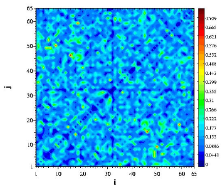
Figure 1: Left: ensemble–averaged second moment of the TBRE (diagonal elements suppressed) for 6 fermions in a single $j=19/2$ shell with total spin $J=12$. Right: same data shown in a histogram.

To lend further substance to these arguments, we have diagonalized the operators $X(\alpha)$ in the space of the 1242 Slater determinants $|i\rangle$ with $J_{z}=0$ (but with no fixed spin) where $i=1,\ldots,D$ with $D=1242$. The eigenstates carry the labels $\alpha$ and $J$ as well as a running label $\mu$ where $\mu=1,\ldots,d_{J}$ and $d_{J}$ is the dimension of the subspace with spin $J$. They are given by $|\alpha J\mu\rangle=\sum_{i=1}^{D}c_{i}(\alpha,J,\mu)|i\rangle$. The complexity of the eigenstates $|\alpha J\mu\rangle$ is measured by the number of principal components ($NPC$) defined as

$$(NPC)^{-1}=\sum_{i=1}^{D}c_{i}^{4}(\alpha,J,\mu).$$ (9)

Table 1 shows the $NPC$s, averaged over all two–body spins (i.e., over all values of $\alpha$) and over all $d_{J}$ states with spin $J$. We recall that the GOE expectation for $NPC$ is $NPC/D=1/3$. We see that the spin–conserving two–body operators $X(\alpha)$ individually yield a strong mixing of the basis states. This mixing is induced entirely by the rotational symmetry and independent of any particular choice of the two–body interaction. It may be argued that the complexity of the coefficients $c_{i}(\alpha,J,\mu)$ reflects just the need to couple the states $|i\rangle$ to total spin $J$, and is not indicative of strong mixing due to $X(\alpha)$. Inspection of the individual coefficients $c_{i}(\alpha,J,\mu)$ shows, however, strong variations with the index $\alpha$ which invalidates this argument. Moreover, calculation of the $NPC$s in a basis with fixed $J$ confirms our picture.

$J$	$d_{J}$	$NPC/D$	$J$	$d_{J}$	$NPC/D$	$J$	$d_{J}$	$NPC/D$
0	10	0.27	1	6	0.27	2	23	0.24
3	21	0.23	4	37	0.24	5	32	0.24
6	49	0.24	7	43	0.24	8	56	0.25
9	51	0.25	10	62	0.25	11	54	0.25
12	65	0.26	13	56	0.26	14	63	0.26
15	55	0.26	16	60	0.26	17	50	0.26
18	55	0.26	19	45	0.26	20	47	0.27
21	39	0.26	22	40	0.27	23	31	0.26
24	33	0.26	25	25	0.26	26	25	0.26
27	19	0.24	28	19	0.24	29	13	0.23
30	14	0.24	31	9	0.22	32	9	0.21
33	6	0.21	34	6	0.21	35	3	0.20
36	4	0.20	37	2	0.18	38	2	0.17
39	1	0.16	40	1	0.15	42	1	0.13

Table 1:

Number of principal components $NPC$ normalized by the dimension $D$ for a system of 6 fermions in a single $j=19/2$ shell. The $NPC$’s are averaged over all two–body spins and over the $d_{J}$ states with spin $J$. The GOE expectation for infinite matrix dimension is 1/3.

We turn to a more complex (and more realistic) shell model consisting of several sub–shells. This situation is typical for nuclei. We distribute $m$ valence nucleons over $q$ single–particle subshells with total angular momenta $j_{k},k=1,\ldots,q$. To simplify the notation, we drop the parity quantum number. The many–body states labelled $\mu$, $\nu$ have spin and isospin quantum numbers $J$ and $T$, respectively. The spin–isospin coupled reduced TBME $V^{st}(j_{k},j_{l};j_{m},j_{n})$ (with $k\leq l$, $m\leq n$, and $s$ and $t$ the two–body spin and isospin, respectively) are labeled $V_{\alpha}$ where $\alpha=1,\ldots,a$ and where $a$ depends upon the particular shell under consideration.

The shell–model Hamiltonian has matrix elements

$$H_{\mu\nu}^{JT}=\sum_{\alpha=1}^{a}V_{\alpha}C_{\mu\nu}^{JT}(\alpha)\ .$$ (10)

Again, the $V_{\alpha}$’s are considered uncorrelated Gaussian–distributed random variables with zero mean value and a common second moment. The matrices $C_{\mu\nu}^{JT}(\alpha)$ contain the geometric aspects of the shell model. Moreover, all ensemble averages (moments and correlation functions of the Hamiltonian and of the Green’s functions) of this TBRE depend only upon the $C_{\mu\nu}^{JT}(\alpha)$’s. Again, it is of central importance to study the properties and the structure of these matrices. Because of the existence of subshells, the matrices $C_{\mu\nu}^{JT}(\alpha)$ exhibit a more complex structure than the EGOE matrices or even the matrices encountered for a single $j$–shell. To understand the structure of these matrices, we use first a qualitative analysis. This analysis applies to the $sd$–shell and to other shells with more than one subshell in heavier nuclei. We label the $JT$–coupled many–body basis states by the occupation numbers $(n_{1},\ldots,n_{q})$ of the $q$ subshells. Here $(n_{1},\ldots,n_{q})$ is a partition of $m$ into $q$ integers, so that $\sum_{k=1}^{q}n_{k}=m$. We assume that the many–body basis states belonging to a given set of quantum numbers $JT$ are ordered in blocks, each block containing states belonging to the same partition. The reduced TBME fall into two classes. The first class consists of the “diagonal” reduced TBME $V^{st}(j_{k},j_{l};j_{k},j_{l})$. These couple only states within the same partition. The matrices $C_{\mu\nu}^{JT}(\alpha)$ corresponding to these TBME are block–diagonal. The second class consists of the “off–diagonal” reduced TBME $V^{st}(j_{k},j_{l},j_{m},j_{n})$ with $(j_{k},j_{l})\neq(j_{m},j_{n})$. These TBME change the occupation numbers $(n_{1},\ldots,n_{q})$ and, thus, couple different partitions. Among these off–diagonal TBME there are those with $k\neq m,n$ and $l\neq m,n$, and those with $k=m$, or $k=n$, or $l=m$, or $l=n$. The former (latter) change the occupation numbers of the subshells by two (one) units, respectively. The matrices $C_{\mu\nu}^{JT}(\alpha)$ corresponding to these off–diagonal reduced TBME have non–zero entries in the off–diagonal blocks only. As a result, the matrix $H_{\mu\nu}^{JT}$ attains a checker–board pattern which reflects the partitions. The pattern is that of $m$ bosons distributed over $q$ single–particle orbitals that interact via two–body interactions.

We display this structure for the particular case of the $sd$–shell with $l=24$ single–particle states, $q=3$ subshells with $j_{1}=5/2$ (for the $d_{5/2}$ sub–shell), $j_{2}=3/2$ (for the $d_{3/2}$ sub–shell, and $j_{3}=1/2$ (for the $s_{1/2}$ sub–shell), occupation numbers $n_{1},n_{2},n_{3}$, and a total of $41$ partitions. Among the $a=63$ reduced TBME, 28 are diagonal, 22 of the off–diagonal reduced TBME induce one–body transitions between the partitions, and 13 transfer two particles. We consider the case of $m=12$ nucleons (“²⁸Si”) in the sector $J=T=0$. The resulting matrix has dimension $839$. All calculations were done using the shell–model code Oxbash [16]. Figure 2 shows the matrix structure (non–zero matrix elements only) of the Hamiltonian (10). The partition structure and the resulting checker–board pattern are clearly visible.

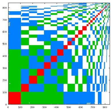
Figure 2: Non–zero matrix elements of the $sd$–shell many–body Hamiltonian with $m=12$ nucleons (“²⁸Si”) in the sector $J=T=0$. Matrix elements originating from diagonal reduced two–body matrix elements are red. Matrix elements originating from off–diagonal reduced two–body matrix elements that transfer one (two) particles between partitions are green (blue).

To elucidate further the structure of the shell–model Hamiltonian of Eq. (10), we ask: How many matrices $C_{\mu\nu}^{JT}(\alpha)$ yield a non–zero contribution to a given matrix element $H_{\mu\nu}^{JT}$? A matrix element of the diagonal blocks gets on average non–zero contributions from $25.2\pm 4.0$ of the 28 block–diagonal matrices corresponding to the diagonal reduced TBME. For the off–diagonal–block matrices corresponding to off–diagonal reduced TBME, the numbers are $7.2\pm 1.4$ out of 22 and $2.0\pm 0.9$ out of 13 for those transferring one and two particles between different partitions, respectively. This shows that in its non–zero blocks, each of the individual matrices $C_{\mu\nu}(\alpha)$ is rather densely populated, and that the density decreases with increasing number of transferred particles.

Further insight into the structure of the Hamiltonian (10) is obtained when we confine attention to the block–diagonal matrices $C_{\mu\nu}(\alpha)$ associated with diagonal TBME. Similar to what was done for the TBRE for a single $j$–shell, we diagonalize these matrices and compute the average number of principal components ($NPC$), i.e. the inverse of the sum over the expansion coefficients raised to the fourth power [3], for each partition. The average is taken over all eigenstates within one partition and over the ensemble of block–diagonal matrices $C_{\mu\nu}(\alpha)$ and is shown in Table 2. We recall that for the GOE and in the limit of infinite matrix dimension $D$, the value would be $NPC/D=1/3$: a typical GOE eigenstate has significant overlap with about $1/3$ of the basis states. Table 2 shows that $NPC/D$ amounts to between 25% and 70% of the GOE expectation for the partitions with dimension $D>20$. The partitions with smaller dimensions yield even higher values for $NPC/D$, but the fluctuations typically increase with decreasing dimension. The degree of mixing tends to decrease with increasing dimension of the partitions although there are considerable fluctuations. We conclude that each diagonal reduced TBME thoroughly mixes the states belonging to a fixed partition. To fully appreciate these statements, the reader should recall that the matrices $C_{\mu\nu}(\alpha)$ do not carry any specific information on the two–body interaction and are determined exclusively by the symmetries of the problem (exclusion principle and conserved quantum numbers $J$ and $T$). The mixing within each partition is expected to be even stronger when we consider a generic two–body interaction and the resulting superposition of matrices $C_{\mu\nu}^{JT}(\alpha)$ in Eq. (10).

Partition	$D$	$NPC/D$
$(6,4,2)$	103	0.10
$(7,3,2)$	67	0.11
$(5,5,2)$	67	0.14
$(5,4,3)$	56	0.18
$(7,4,1)$	56	0.09
$(6,3,3)$	53	0.15
$(6,5,1)$	53	0.13
$(8,2,2)$	35	0.20
$(4,6,2)$	35	0.21
$(4,5,3)$	34	0.23
$(8,3,1)$	34	0.14
$(7,2,3)$	27	0.22
$(5,6,1)$	27	0.24

Table 2:

Number of principal components $NPC$ normalized by the dimension $D$ for the 13 largest partitions generated by mixing due to the block–diagonal matrices $C_{\mu\nu}(\alpha)$. The GOE expectation for infinite matrix dimension is 1/3.

Although the mixing between partitions is not as strong as that within each partition, $H_{\mu\nu}^{JT}$ will, for ²⁸Si and $J=0$ $T=0$, generically generate chaos. To show this, we have compared our Figure 2 with the corresponding figure for the Wildenthal two–body interaction (which was used in Ref. [3] and shown there to produce chaos; see, e.g., Figs. 23(a) and 23(c) of that reference). The two figures are indistinguishable.

4 Discussion and Summary

The aims and results of our paper can be summarized from two points of view, from that of random–matrix theory and from that of nuclear structure theory.

From the viewpoint of random–matrix theory, we have compared three random–matrix ensembles that have been used in the past to deal with interacting many–body systems and, in particular, with nuclei: The GOE, the EGOE(2), and the TBRE, the latter applied to a single $j$–shell and to the $sd$–shell. In our comparison, we have emphasized the central role of the structure matrices denoted by $D^{\rm GOE}$, $D$, $C^{J}$, and $C^{JT}$, respectively. These matrices provide the scaffolding of the underlying random–matrix ensemble. Averages, higher moments and correlation functions of all observables can be expressed in terms of and are completely determined by these matrices. These matrices then must form the central object of study of the said random–matrix ensembles.

In the framework of a many–body problem, use of the GOE is tantamount to assuming many–body forces the rank of which equals the number of valence particles. This unrealistic aspect of the GOE has to be weighed against the great advantage of its structural simplicity. This simplicity is due to the orthogonal invariance of the GOE. It allows for a complete analytical calculation of all moments and correlation functions. Hence the predictive power of the GOE. The orthogonal invariance manifests itself in the large number ($\propto N^{2}$ with $N$ the matrix dimension) of independent random variables and in the extreme simplicity of the structural matrices $D^{\rm GOE}$. In the GOE, no reference is made to the possible existence of quantum numbers like spin or isospin.

The EGOE(2) is designed to deal with many–body systems which are governed by two–body forces. In this respect the EGOE(2) is a much more realistic model than the GOE. The model does not possess the orthogonal invariance of the GOE. This is why all attempts at calculating spectral fluctuations analytically for this ensemble have failed so far. For the same matrix dimension, the number of uncorrelated random variables is much smaller than in the GOE. To achieve complete mixing of the basis states, this reduction must be made up for by a greater complexity of the matrices $D$. We have displayed the structure of these matrices which individually are quite sparse but jointly provide for strong mixing of the basis states. Like the GOE, the EGOE(2) does not allow for the possible existence of quantum numbers like spin or isospin.

The TBRE is more realistic yet than the EGOE(2) in that it does take account of the two essential properties of the residual interaction of the nuclear shell model: The interaction is a two–body interaction, and it preserves spin, parity, and isospin. The existence of symmetries associated with these quantum numbers has an essential influence on the structure of the ensemble and of the matrices $C^{J}$ and $C^{JT}$ which embody this structure: Compared to the EGOE(2) with the same matrix dimension, the number of independent random variables is much reduced once again, but the complexity of the matrices $C^{J}$ and $C^{JT}$ is much increased. It appears that the TBRE is even harder to deal with than the EGOE(2). In any case, we are not aware of any previous attempts to study this ensemble analytically. In the TBRE for a single $j$–shell, the non–commuting matrices $C^{J}$ have strong diagonal elements (a feature already encountered for the EGOE(2) and related to sum rules). The non–diagonal elements are not sparse but, on the contrary, dense. This is how a complete mixing of the basis states is achieved in the $j$–shell TBRE. In the $sd$–shell TBRE, the existence of sub–shells and the associated block structure of the matrices $C^{JT}$ lends greater complexity yet to the ensemble. Mixing is very strong within the diagonal blocks and weaker for the off–diagonal ones. In both these ensembles, symmetries play an important role and, together with the exclusion principle, define the structure of the matrices $C^{J}$ and $C^{JT}$. It goes without saying that the relevant symmetry operators must not from a complete set of commuting operators as otherwise there would be no room left for a random–matrix ensemble.

From the point of view of nuclear structure theory, we have uncovered generic features of shell–model calculations. These are embodied in the matrices $C^{J}$ and $C^{JT}$. Every shell–model calculation for a single $j$–shell or for the $sd$–shell amounts to choosing a specific linear combination of these matrices (the same for every value of spin $J$), and diagonalizing the resulting Hamiltonian matrix. Corresponding statements apply for other shells. Inasmuch as there is evicence for chaos in one such calculation using a specific set of two–body matrix elements, the properties of the matrices $C^{J}$ and $C^{JT}$ displayed above guarantee that spectra and eigenfunctions calculated for most other choices of the two–body interaction will likewise be chaotic. The two–body interactions for which this statement does not apply form a set of measure zero.

It is in this sense that we have demonstrated that chaos is a generic property of the nuclear shell–model. We have also shown that symmetries (which are due to the existence of an incomplete set of commuting operators) determine the structure of the TBRE in an essential way. Thus, such symmetries are vital for the occurrence of chaos in the TBRE. Another aspect of our work (not emphasized in the present paper but a natural spin–off) is the existence of correlations between many–body spectra having different quantum numbers like total spin $J$. It is immediately obvious from Eqs. (8) and (10) that Hamiltonian matrices pertaining to different spin values in the same nucleus are correlated since they depend on the same set of random variables. This fact has been used to explain the observed preponderance of spin–zero ground states in calculations using the TBRE [17].

Our considerations are restricted to spherical nuclei and totally degenerate major shells. We have remarked in the Introduction that lifting this degeneracy by taking into account the differences of the single–particle energies in individual sub–shells, will drive the system toward regularity. Our considerstions do not apply to deformed nuclei. Here the Nilsson model provides a single–particle basis in which it is meaningless to assume degenerate single–particle energies. Such nuclei possess well–developed collective motion. However, collective motion exists also beyond the regime of well–deformed nuclei. It has been notoriously difficult in the past to understand this fact in the framework of the spherical shell model, with the exception of certain types of collectivity like that of the giant dipole resonance. Understanding both, collectivity and chaos, within a common framework is, thus, a goal of future work. We observe, however, that collectivity typically involves levels with different quantum numbers (like those forming a rotational band) while chaos is a property displayed by levels with identical quantum numbers. Thus, in nuclei chaos and collectivity need not be antagonistic.

Appendix

In the framework of the TBRE for a single $j$–shell, we derive Eq. (6), and we define the operators $X(\alpha)$. The calculation of $N(J)$, the number of many–body states with spin $J$, is rather standard. We first calculate the number $n(M)$ of states with $J_{z}=M$ and then $N(J)$ from the identity $N(J)=n(J)-n(J+1)$. We focus attention on large values of $m$ and $j$, $m\gg 1$ and $j\gg 1$. We have

$$n(M)=\sum_{-j\leq\mu_{1}<\mu_{2}<\ldots<\mu_{m}\leq j}\delta(M-\sum_{i=1}^{m}\mu_{i})\ .$$ (11)

Here the delta symbol stands for a Kronecker delta and not for the Dirac delta function. We write the sum as

$$n(M)=\frac{1}{m!}\sum_{-j\leq\mu_{1},\mu_{2},\ldots,\mu_{m}\leq j}\bigg{(}\prod_{k<l}[1-\delta_{\mu_{k}\mu_{l}}]\bigg{)}\delta(M-\sum_{i=1}^{m}\mu_{i})\ .$$ (12)

We expand the product in powers of the Kronecker deltas and consider first the term of zeroth order $n_{0}(M)$, i.e., the term with only one constraint ($M=\sum\mu_{i}$). It is

$$n_{0}(M)=\frac{1}{m!}\sum_{\mu_{1}=-j}^{j}\sum_{\mu_{2}=-j}^{j}\times\ldots\times\sum_{\mu_{m}=-j}^{j}\delta(M-\sum_{i=1}^{m}\mu_{i})\ .$$ (13)

The Kronecker delta is written as $\delta_{l,0}=(1/(2\pi))\int_{-\pi}^{+\pi}\exp[il\phi]{\rm d}\phi$. This yields

$$n_{0}(M)=\frac{1}{2\pi m!}\int_{-\pi}^{+\pi}{\rm d}\phi\sum_{\mu_{1},\mu_{2},\ldots,\mu_{m}=-j}^{j}\exp[i\phi(M-\mu_{1}-\mu_{2}-\ldots-\mu_{m})]\ .$$ (14)

The summation yields

$$n_{0}(M)=\frac{1}{2\pi m!}\int_{-\pi}^{+\pi}{\rm d}\phi\ \cos[\phi M]\biggl{(}\frac{\sin[(j+1/2)\phi]}{\sin\phi/2}\biggr{)}^{m}\ .$$ (15)

We replace $\phi$ by $x=j\phi$ and use that $j\gg 1$. Then the function

$$\bigg{(}\frac{\sin[(1+1/(2j))x]}{\sin[x/(2j)]}\bigg{)}^{m}$$ (16)

has maxima at $x=0$, $x=\pm 3\pi/2$, $x=\pm 5\pi/2$, $\ldots$ with absolute values $(2j)^{m}$, $(2j)^{m}(2/(3\pi))^{m}$, $(2j)^{m}(2/(5\pi))^{m}$, $\ldots$. For $m\gg 1$, the maximum at $x=0$ gives the dominating contribution. We take account of this maximum only and write

$$\biggl{(}\frac{\sin[(1+1/(2j))x]}{\sin[x/(2j)]}\biggr{)}^{m} = \exp\bigg{\{}m\ln\sin[(1+1/(2j))x]-m\ln\sin[x/(2j)]\bigg{\}}$$ (17)

$$\qquad\approx(2j+1)^{m}\exp\{-(m/6)x^{2}\}\ .$$

In the exponent we have omitted terms of higher order than the first in $x^{2}$. This is justified because upon using a Taylor expansion and performing the Gaussian integration, such terms will produce inverse powers of $m$ and are, therefore, negligible. Thus, our procedure amounts to an asymptotic expansion in inverse powers of $j$ and $m$. Hence,

$$n_{0}(M) \approx \frac{(2j+1)^{m}}{2\pi jm!}\int_{-\infty}^{\infty}{\rm d}x\ \cos[Mx/j]\exp\{-(m/6)x^{2}\}$$ (18)

$$= \frac{(2j+1)^{m}}{2\pi jm!}\sqrt{\frac{6\pi}{m}}\exp\big{\{}-\frac{3M^{2}}{2mj^{2}}\big{\}}\ .$$

We turn to the terms which are linear in the Kronecker delta’s in Eq. (12). Their sum is denoted by $n_{1}(M)$ and can be calculated along quite similar lines. In the same asymptotic limit we find

$$n_{1}(M)\approx-\frac{m^{2}n_{0}(M)}{2(2j+1)}\ .$$ (19)

This shows that $n_{1}(M)$ is negligible in comparison with $n_{0}(M)$ if $j\gg m$. That same statement holds a fortiori for the contributions which are of higher order in the Kronecker delta’s. Thus, $n(M)\approx n_{0}(M)$, and $N(J)=n(J)-n(J+1)$ then gives the result (6).

We come to the definition of the operators $X(\alpha)$. Let $a_{\rho}$ and $a^{\dagger}_{\rho}$ be the destruction and creation operators for a fermion in a state with $j_{z}$–component $\rho$ with $\rho=-j,\ldots,j$. When acting upon the vacuum state, the operators

$$(A^{s}_{M})^{\dagger}=\sum_{\rho}c(jjs;\rho,M-\rho)a^{\dagger}_{\rho}a^{\dagger}_{M-\rho}$$ (20)

create a pair of fermions coupled to total spin $s$ and $z$–component $M$. Here, $s=0,2,4,\ldots,2j-1$. The Hermitean conjugate operators are

$$A^{s}_{M}=-\sum_{\rho}c(jjs;\rho,M-\rho)a_{\rho}a_{M-\rho}\ .$$ (21)

The scalar operators

$$X(s)=(1/2)\sum_{M}(A^{s}_{M})^{\dagger}A^{s}_{M}$$ (22)

describe the interaction of two fermions coupled to spin $s$. With $\alpha=(1/2)s+1$, these are the operators $X(\alpha)$ introduced in Eq. (7). From an identity for the Clebsch–Gordan coefficients, it follows trivially that

$$\sum_{s}X(s)=(1/2){\hat{n}}({\hat{n}}-1)\ .$$ (23)

This is the relation used below Eq. (7). For $s\neq t$, the commutator $[X(s),X(t)]$ does not vanish and has the from of a three–body interaction term. Since the projection operators ${\bf P}(J)$ trivially commute with $X(s)$ for all $J$ and $s$, the commutator of two operators ${\hat{C}}$ with $\alpha\neq\beta$ is

$$[{\hat{C}}^{J}(\alpha),{\hat{C}}^{J}(\beta)]={\bf P}(J)[X(\alpha),X(\beta)]{\bf P}(J)$$ (24)

and it follows that the ${\hat{C}}$’s likewise do not commute.

References

- [1] R. U. Haq, A. Pandey, and O. Bohigas, Phys. Rev. Lett. 48, 1086 (1982); O. Bohigas, R. U. Haq, and A. Pandey, in Nuclear Data for Science and Technology, K. H. Böchhoff (Ed.), Reidel, Dordrecht (1983).
- [2] G. E. Mitchell, E. G. Bilpuch, P. M. Endt, and F. J. Shriner, Jr., Phys. Rev. Lett. 61, 1473 (1988); F. J. Shriner, Jr., E. G. Bilpuch, P. M. Endt, and G. E. Mitchell, Z. Phys. A 335, 393 (1990).
- [3] V. Zelevinsky, B. A. Brown, N. Frazier, and M. Horoi, Phys. Rep. 276, 85 (1996).
- [4] A. Abul–Magd, M. Simbel, H.–L. Harney, and H. A. Weidenmüller, Phys. Lett. B 579, 278 (2004), nucl-th/0212057.
- [5] V. V. Flambaum, A. A. Gribakina, G. F. Gribakin, and M. G. Kozlov, Phys. Rev. A 50, 267 (1994).
- [6] S. C. Pieper, R. B. Wiringa, Ann. Rev. Nucl. Part. Sci. 51, 53 (2001), nucl-th/0103005.
- [7] J. B. French and S. S. M. Wong, Phys. Lett. B 33, 449 (1970).
- [8] O. Bohigas and J. Flores, Phys. Lett. B 34, 261 (1971).
- [9] K. K. Mon and J. B. French, Ann. Phys. (NY) 95, 90 (1975).
- [10] V. K. B. Kota, Phys. Rep. 347, 223 (2001).
- [11] L. Benet and H. A. Weidenmüller, J. Phys. A 36, 3569 (2003), cond-mat/0207656.
- [12] J. J. M. Verbaarschot and P. J. Brussaard, Phys. Lett. 87 B (1979) 155.
- [13] L. Benet, T. Rupp, H. A. Weidenmüller, Phys. Rev. Lett. 87, 010601 (2001), cond-mat/0010425; Ann. Phys. 292, 67 (2001), cond-mat/0010426.
- [14] M. Srednicki, Phys. Rev. E 66, 046138 (2002), cond-mat/0207201.
- [15] Y. V. Fyodorov und A. D. Mirlin, J. Phys. A 24, 2273 (1991).
- [16] B. A. Brown, A. Etchegoyen, and W. D. M. Rae, The computer code OXBASH, MSU-NSCL report number 524 (1988).
- [17] T. Papenbrock and H. A. Weidenmüller, Phys. Rev. Lett. 93 (2004) 132503, nucl-th/0404022.