Statistical fluctuations of ground–state energies and binding energies in nuclei

Abstract

The statistical fluctuations of the ground–state energy and of the binding energy of nuclei are investigated using both perturbation theory and supersymmetry. The fluctuations are induced by the experimentally observed stochastic behavior of levels in the vicinity of neutron threshold. The results are compared with a recent analysis of binding–energy fluctuations by Bohigas and Leboeuf, and with theoretical work by Feshbach et al.

Introduction. In this letter, we address the question: How does the interaction with high–lying configurations affect the properties of nuclear ground states? In particular, what are the ensuing uncertainties, given the fact that not much is known about both, the interaction and the high–lying configurations? The question has arisen within two seemingly different contexts. (i) In a purely theoretical framework, and inspired by the analogy with the theory of the optical model (where averaging over the random fluctuations of the compound–nucleus resonances is an essential element), the question was addressed using a statistical model for the high–lying states. To this end, Feshbach’s projection operator method [1] has been extended to the bound–state problem and used to estimate the resulting uncertainties in ground–state energies and wave functions [2]. (ii) A series of ever–refined nuclear mass formulas with a sizeable number of parameters has been used to fit the known binding energies. In spite of many years of dedicated effort, there remains a difference between mass formulas and data: The data fluctuate about the (smooth) best fits. The fluctuations have a width of about $0.5$ MeV and have been interpreted as being due to chaotic nuclear motion [3]. Since the spectral fluctuations of nuclear levels near neutron threshold (and near the Coulomb barrier for protons) follow random–matrix predictions [4], the question arises whether this fact can be used to account for the observed fluctuations.

We present a novel statistical approach to the question formulated above. In contrast to Refs. [2], it is not our aim to estimate the theoretical uncertainty of nuclear binding energies resulting from the use of a mean–field approach. Rather, we are interested in the statistical fluctuations of ground–state and binding energies which are induced by those of high–lying configurations. These represent genuine theoretical uncertainties which are quite independent of the particular approach used to calculate nuclear properties. To this end we describe the high–lying configurations in terms of a random–matrix model. In trying to be as conservative as possible, we only use the fact just mentioned that in many nuclei with mass number $A>30$ or so, random–matrix theory correctly describes the statistical fluctuations of states at excitation energies of 8 to 10 MeV. We show that from this input it is possible to estimate the minimum statistical uncertainties in nuclear ground–state energies and, from there, nuclear binding energies. We compare our results with the work of Refs. [2], and with the empirical results of Ref. [3].

Model. Starting point is the nuclear shell model. Neighboring major shells are separated by an energy difference $\hbar\omega\approx 41/A^{1/3}$ MeV. We first neglect the mixing between major shells due to the residual interaction. Then, the nuclear ground state is obtained by diagonalizing the shell–model Hamiltonian (which consists of the single–particle energies of the lowest shell and of the matrix elements of the residual interaction with respect to many–body states in that shell). The resulting ground state has energy $E_{0}$. The corresponding eigenfunction is composed of configurations belonging to the lowest major shell. We assume that the residual interaction within the states of each of the remaining major shells (excitation energies $n\hbar\omega$ with $n=1,2,\ldots$) is so strong as to completely mix the configurations within that shell. Then, the spectra and eigenfunctions within each such shell are described by random–matrix theory, more precisely: by the Gaussian orthogonal ensemble (GOE) of random matrices. For $n\geq 1$, this assumption is consistent with the spectral fluctuations analyzed in Ref. [4], and with the properties of nuclear cross–section fluctuations at higher excitation energies [5]. The resulting nuclear spectrum is schematically depicted in Fig. 1.

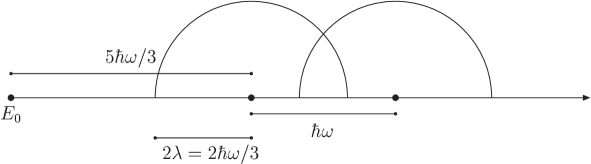
Figure 1: Schematic representation of the nuclear spectrum in the shell model. The semicircles represent the shells with $n=1$ and $n=2$.

Each of the higher shells ($n\geq 1$) gives rise to a Gaussian–shaped mean level density. In what follows we replace each Gaussian by the semicircle characteristic of random–matrix theory. For our order–of–magnitude estimates, the difference should be irrelevant. We focus attention on the shell with $n=1$ and later show that higher shells do not affect the result significantly. We estimate the shift and the uncertainty of the ground–state energy $E_{0}$ using (i) perturbation theory, (ii) the supersymmetry approach. Here, $E_{0}<0$ is the difference between the location of the ground state and the center of the shell with $n=1$. The semicircle has radius $2\lambda$. Estimates for $E_{0}$ and of $\lambda$ are given below. For simplicity, we focus attention entirely on the ground state and omit the other states in the shell with $n=0$.

Perturbation Theory. We denote by $V_{0j}$ the matrix elements of the residual interaction connecting the ground state with the states $j=1,\ldots,N$ in the major shell with $n=1$, and by $E_{j}$ the GOE eigenvalues in that shell, counted from the center. For $N$, the number of states in that shell, we have $N\gg 1$. The energy $\tilde{E_{0}}$ of the perturbed ground state is given by

$$\tilde{E_{0}}=E_{0}+\sum_{j=1}^{N}\frac{V^{2}_{0j}}{E_{0}-E_{j}}+\ldots\ \ .$$ (1)

Within the GOE, the $V_{0j}$’s and the $E_{j}$’s are uncorrelated random variables. The $V_{0j}$’s are Gaussian distributed with zero mean value. Using the standard definition $\Gamma^{\downarrow}=2\pi\overline{V^{2}_{0j}}/d$ of the spreading width for mixing of the ground–state wave function with the states of the $n=1$ shell, we write the second moment $\overline{V_{0j}V_{0k}}=(1/(2\pi))\Gamma^{\downarrow}d\ \delta_{jk}$. Here, $d=\pi\lambda/N$ is the mean level spacing in the $n=1$ shell. Averaging Eq. (1) over the GOE, we find to lowest order in $\Gamma^{\downarrow}$,

$$\overline{\tilde{E_{0}}}\approx E_{0}+\frac{\Gamma^{\downarrow}d}{2\pi}\int{\rm d}E^{\prime}\frac{1}{E_{0}-E^{\prime}}\overline{\sum_{j}\delta(E^{\prime}-E_{j})}\ .$$ (2)

By definition, $\overline{\sum_{j}\delta(E^{\prime}-E_{j})}$ is equal to $\overline{\rho(E^{\prime})}$, the average level density normalized to $N$. Hence we find approximately

$$\overline{\tilde{E_{0}}}\approx E_{0}+\frac{\Gamma^{\downarrow}\lambda}{2E_{0}}\ .$$ (3)

The level shift $\Gamma^{\downarrow}\lambda/(2E_{0})$ is negative, as expected. To calculate the variance, we define $\overline{\rho(E_{1},E_{2})}=\sum_{jk}\overline{\delta(E_{1}-E_{j})\delta(E_{2}-E_{k})}$ and use the fact that the correlation function $\overline{\rho(E_{1},E_{2})}-\overline{\rho(E_{1})}\ \overline{\rho(E_{2})}$ tends to zero over distances $|E_{1}-E_{2}|$ that are of order $d$ (and not $Nd$). Proceeding as before, we find

$$\overline{(\tilde{E_{0}}-E_{0})^{2}}-\biggl{(}\overline{\tilde{E_{0}}}-E_{0}\biggr{)}^{2}=\frac{c}{N}\biggl{(}\frac{\Gamma^{\downarrow}\lambda}{2E_{0}}\biggr{)}^{2}\ .$$ (4)

Here $c$ denotes a constant of order unity (and not of order $N$). We observe that with $N\gg 1$, the fluctuations are much smaller than the level shift. Rough estimates are obtained by putting $2\lambda\approx(2/3)\hbar\omega$ (the semicircles of the shells $n$ and $n+1$ overlap), $E_{0}\approx-(5/3)\hbar\omega$, and $\Gamma^{\downarrow}\approx 3$ MeV. The last figure roughly corresponds to the spreading width of the giant dipole resonance which accounts for the mixing of one–particle one–hole and two–particle two–hole configurations and is, thus, similar to the mixing of the ground–state wave function with the wave functions in the shell with $n=1$ considered here. For the shift, this yields a typical value of $-0.3$ MeV. The r.m.s. fluctuation is roughly given by that value divided by $\sqrt{N}$. To estimate $N$ we use $N=\pi\lambda/d_{t}$. Here $d_{t}$ is the mean level spacing at neutron threshold. For heavy nuclei, $d_{t}\approx 10$ eV, $\hbar\omega\approx 6.5$ MeV, and $N\approx 10^{6}$ while for nuclei with mass number $A$ around 50 we have $d_{t}\approx 10$ keV, $\hbar\omega\approx 10$ MeV and $N\approx 10^{3}$. We find that the r.m.s. fluctuation is about 0.3 keV for heavy nuclei and about 10 keV for nuclei with $A\approx 50$. These figures are order–of–magnitude estimates only, of course.

Supersymmetry. We use the supersymmetry method (SUSY)[6, 7] in order to show that the perturbative estimates given above essentially remain valid beyond the domain of perturbation theory. The calculations are rather technical and cannot be given here. A more detailed account is in preparation [8]. Suffice it to say that using SUSY and $N\gg 1$, we find the following saddle–point equation for the $\sigma$ matrix of the one–point function:

$$\sigma=\frac{\lambda}{E-\lambda\sigma}+\frac{1}{N}\ \frac{\lambda}{E-\lambda\sigma-(1/2)\Gamma^{\downarrow}\lambda/(E-E_{0})}\ .$$ (5)

Here the first term on the r.h.s. is the usual contribution which, taken by itself, results in the semicircle law. (We recall that the spectrum is located in that energy interval where $\sigma$ has non–real values, with the average level density proportional to ${\rm Im}\ \sigma$). The second term is the correction due to the coupling with the ground state. This term yields an additional contribution to ${\rm Im}\ \sigma$ in an energy interval of width $\Delta E$ located at $\tilde{E_{0}}$ outside the semicircle and in the vicinity of $E_{0}$. We solve Eq. (5) for the diagonal elements of the $\sigma$ matrix using perturbation theory. For the shift, we retrieve our previous result, Eq. (3). For $\Delta E$ we find

$$\Delta E=\frac{1}{N^{1/2}}\ \frac{\Gamma^{\downarrow}\lambda}{2|E_{0}|}\ \frac{4\lambda}{|E_{0}|}\ .$$ (6)

This agrees with Eq. (4) except for the last factor. This factor is of order unity. It arises because in Eqs. (4) and (6), we have calculated different expressions (the r.m.s. fluctuation and the width of the spectrum, respectively). We have used Eq. (5) also to calculate shift and width non–perturbatively for values of $E_{0}$ close to the edge of the semicircle. We have found that these values differ from the perturbative ones only by numerical factors. We conclude that our estimates in Eqs. (3) and (5) are approximately valid in a wide range of values for $E_{0}$ and $\Gamma^{\downarrow}$.

Discussion. So far, only the influence of the shell with $n=1$ on the ground–state energy has been taken into account. What about higher shells ($n>1$)? Since SUSY has corroborated the perturbative results, we may safely use perturbation theory to answer the question. Formally, Eqs. (3) and (4) remain valid, with $E_{0}$ replaced by the distance $D_{n}$ between the energy of the ground state and the center of the shell $n$ under consideration, and $\Gamma^{\downarrow}$ replaced by $\Gamma^{\downarrow}_{n}$, the spreading width describing the mixing of the ground–state wave function with the configurations in shell $n$. While $(D_{n})^{-1}$ decreases only like $n^{-1}$, $\Gamma^{\downarrow}_{n}$ falls off very rapidly (exponentially). This is because $\Gamma^{\downarrow}$ depends partly upon the overlap between the ground–state wave function and the configurations in shell $n$. In a different context, this exponential fall–off has been demonstrated numerically in Figure 1 of Ref. [9] where the dependence of the ground–state energy upon the truncation of the shell–model space was studied. Therefore, we expect that the inclusion of higher shells would affect our estimates only by a factor two or three or so. It is possible, of course, that our treatment is too conservative, and that the domain where the GOE applies, extends further down in the spectrum. This would reduce $|E_{0}|$ and $N$ and, thus, enhance both the shift and the r.m.s. fluctuation. Unfortunately, there is hardly any empirical evidence one way or another concerning that problem. In summary, we find that the shift of the ground–state energy is of the order of or larger than 0.5 to 1 Mev for all nuclei, while the fluctuations amount at least to several 10 keV (1 keV) for medium–weight (heavy) nuclei, respectively. It goes without saying that these fluctuations do not describe actual fluctuations of the ground–state energy, but rather the minimum theoretical uncertainty due to lack of precise information about the states and interactions in the shells with $n\geq 1$.

So far we have considered only a single level rather than the complete set of states belonging to the lowest shell. We do not expect that the presence of these states strongly affects our estimates. To be sure that this is indeed the case, we should also derive and solve the saddle–point equation for this case. This work is now under way [8].

How are our results related to those of Refs. [2]? The problem addressed in Refs. [2] was not to compute the r.m.s. fluctuations, but rather to relate the theoretical uncertainty of the binding energy per nucleon to that of the mean–field energy and to that of the residual interaction (the difference between the true interaction and the mean field). The latter connects the mean–field ground state to the excited states. This was done in the framework of a somewhat simpler problem, the energy per particle of nuclear matter, rather than for finite nuclei.

In most nuclei, the mean–field energy differs from the energy denoted by $E_{0}$ in the present paper. Indeed, our definition of $E_{0}$ includes the effects of the residual interaction within the lowest shell and differs, therefore, from the mean–field energy. Moreover, we focus attention on stochastic uncertainties resulting from the chaotic behavior of excitet states in the vicinity of neutron threshold. We do not attempt to estimate the error that comes with a theory based upon a mean–field approach. Therefore, the approach of Refs. [2] and the one used here, are rather different, and a direct comparison of the results is not possible.

Fluctuations of Binding Energies. How can we use our results to estimate the fluctuations in the binding energies of nuclei? The binding energy is the minimum excitation energy at which the nucleus fragments into $A$ separate nucleons. We do not believe that it is possible at present to determine this excitation energy reliably in the framework of a nuclear–structure calculation for nucleus $A$. Indeed, to the best of our knowledge, nuclear–structure calculations have rarely been used to calculate binding energies, except for the lightest nuclei. To answer the questions raised in Ref. [3], we use the following indirect approach. Our calculations yield the fluctuation of the nuclear ground–state energy with respect to the center of the shell with $n=1$. For most nuclei, the threshold for neutron or for proton emission lies somewhere in that shell. Thus, we identify the calculated fluctuation with the fluctuation of the ground–state energy with respect to neutron (or proton) threshold. The fluctuation of the nuclear binding energy is then obtained by the combined effect of removing successively $A$ nucleons from the nucleus.

We apply this scheme in reverse order, starting from a nucleus with mass number $A_{0}$ and adding $A-A_{0}$ nucleons to it. The first nucleus (in increasing order of $A$) where we have definitive evidence (both experimentally and theoretically) that GOE statistics applies is ²⁶Al [10, 11]. We assume that nuclei with mass numbers $A\leq 25$ do not have any fluctuations in either ground–state or binding energy. Therefore, we choose $A_{0}=26$ and an initial value 30 keV for the fluctuation of the ground–state energy and, thus, of the binding energy. To calculate the fluctuations of the binding energy for nuclei with mass numbers $A>A_{0}$ we assume, for simplicity, that the fluctuations of the ground–state energy have a Gaussian distribution. (In the framework of our model, this may or may not be the case. We have not explored the solutions of the saddle–point equation to the point of ascertaining the answer to this question but recall that for the main part of the spectrum, the distribution has the shape of a semicircle and not of a Gaussian. Such details should, however, be irrelevant for a rough estimate). Under this assumption, the fluctuation of the binding energy of a nucleus with $A$ nucleons is obtained by the convolution of $(A-A_{0})$ Gaussian distributions, each with its own $A$–dependent width. The resulting distribution is again Gaussian. Its variance $(\sigma_{A})^{2}$ is the sum of the variances of the individual Gaussians, the latter being given by the $A$–dependent r.h.s. of Eq. (4). Thus,

$$(\sigma_{A})^{2}=(30\ {\rm keV})^{2}+\sum_{A^{\prime}=A_{0}+1}^{A}\frac{c}{N}\biggl{(}\frac{\Gamma^{\downarrow}\lambda}{2E_{0}}\biggr{)}^{2}\ .$$ (7)

Eq. (7) holds provided that the fluctuations in different nuclei are statistically uncorrelated. We are not aware of any evidence to the contrary. The most significant dependence upon $A^{\prime}$ on the r.h.s. of Eq. (7) resides in $N=\pi\lambda/d$. Since $N$ increases strongly (nearly exponentially) with $A$, the individual terms under the sum decrease rapidly, and $\sigma_{A}$ is a monotonically increasing function of $A$ with ever decreasing slope. This statement applies in general, quite irrespective of any details of the $A$–dependence of $N$. We roughly model the $A$–dependence of the terms under the sum by writing

$$\frac{c}{N}\biggl{(}\frac{\Gamma^{\downarrow}\lambda}{2E_{0}}\biggr{)}^{2}\approx(30\ {\rm keV})^{2}\exp(\sqrt{A_{0}}-\sqrt{A})\ .$$ (8)

This formula takes account of the initial condition at $A_{0}=26$ and models the $A$–dependence in terms of the exponential which roughly reflects the dependence of the average level density on $A$. (A more precise expression would have $\exp\sqrt{A}$ replaced by $\exp[\alpha\sqrt{A}]$, with $\alpha$ of order unity and weakly dependent on $A$. We disregard such corrections in view of the rather rough overall approach we have taken). We use this expression in Eq. (7), replace the summation by an integration, and obtain

$$\sigma(A)=(30\ {\rm keV})\biggl{[}1+2(\sqrt{A_{0}}+1)(1-\frac{\sqrt{A_{0}}+1}{\sqrt{A}+1}\exp\{\sqrt{A_{0}}-\sqrt{A}\})\biggr{]}^{1/2}\ .$$ (9)

Figure 2: Fluctuations of nuclear ground–state energies. Dashed curve: fit to the experimental data taken from Ref. [12]; dot–dashed curve: formula (9) of the text; continuous curve: formula (9) with the factor 30 replaced by 120 $keV$.

In Figure 2, we compare our Eq. (9) with the result reported in Ref. [3] for the fluctuations of the binding energies versus $A$. To emphasize the uncertainties in our estimates, we show two curves, one of which represents Eq. (9) as it stands while for the other, we have arbitrarily replaced the factor 30 keV on the r.h.s. of Eq. (9) by 120 keV. We see that for heavy nuclei, the data and our result have similar values while for $A\approx 50$, the difference is larger. In view of the rather large uncertainties of our estimates, we would be satisfied with an order–of–magnitude agreement and do not attach much significance to such statements. More important, in our view, is the fact that we predict a monotonically increasing function of $A$ while both, the data and the chaotic model of Ref. [3], yield a monotonic decrease with $A$. As for the data, we can think of additional effects that might affect the $A$–dependence. For instance, it is conceivable that for light nuclei, the clean separation between surface terms and volume terms assumed in the mass formulas, does not apply. This might add a correction which strongly decreases with $A$ and which has to be removed from the data before a comparison with our results can be made. Within the conservative phenomenological approach which we have taken, there seems no way of escaping the conclusion that $\sigma_{A}$ increases monotonically with $A$. This is clear from Eq. (7) which, in turn, rests upon our identification of fluctuations of the binding energy of a nucleus with mass number $A$ with the fluctuations of the ground–state energies with respect to neutron or proton threshold of all nuclei with mass numbers $A^{\prime}<A$.

References

- [1] H. Feshbach, Phys. Rep. 264 (1996) 137.
- [2] R. Carraciolo, A. De Pace, H. Feshbach, and A. Molinari, Ann. Phys. (N. Y.) 262 (1998) 105; A. De Pace, H. Feshbach, and A. Molinari, Ann. Phys. (N. Y.) 278 (1999) 109; A. De Pace and A. Molinari, Ann. Phys. (N. Y.) 296 (2002) 263.
- [3] O. Bohigas and P. Leboeuf, Phys. Rev. Lett. 88 (2002) 092502-1; erratum ibid. 129903-1.
- [4] U. Haq et al., Phys. Rev. Lett. 48 (1982) 1086; O. Bohigas et al., in: Nuclear Data for Science and Technology, Reidel (1983) p. 809.
- [5] T. Ericson and T. Mayer–Kuckuk, Ann. Rev. Nucl. Sci. 16 (1966) 183.
- [6] K. B. Efetov, Supersymmetry in Disorder and Chaos, Cambridge University Press 1997; see also Advances in Physics 32 (1983) 53.
- [7] J. J. M. Verbaarschot, H. A. Weidenmüller, and M. R. Zirnbauer, Phys. Rep. 129 (1985) 367.
- [8] A. De Pace, A. Molinari and H. A. Weidenmüller, in preparation.
- [9] V. Zelevinsky and A. Volya, Proceedings of the 7th International Spring Seminar on Nuclear Physics, Maiori, Italy, 2001, World Scientific, Singapore and nucl-th/0112014.
- [10] G. E. Mitchell, E. G. Bilpuch, P. M. Endt, and F. J. Shriner, Jr., Phys. Rev. Lett. 61, 1473 (1988); F. J. Shriner, Jr., E. G. Bilpuch, P. M. Endt, and G. E. Mitchell, Z. Phys. A 335, 393 (1990).
- [11] V. Zelevinsky, B. A. Brown, N. Frazier, and M. Horoi, Phys. Rep. 276 (1996) 85.
- [12] P. Möller, J.R. Nix, W.D. Myers and W.J. Swiatecki, At. Data Nucl. Data Tables 59, 185 (1995)