Is friction responsible for the reduction of fusion rates far below the Coulomb barrier?

Abstract

The fusion of two interacting heavy ions traditionally has been interpreted in terms of the penetration of the projectile into the target. Observed rates well below the Coulomb barrier are considerably lower than estimates obtained from penetration factors. One approach in the analysis of the data invokes coupling to non-elastic channels in the scattering as the source of the depletion. Another is to analyze those data in terms of tunneling in semi-classical models, with the observed depletion being taken as evidence of a “friction” under the barrier. A complementary approach is to consider such tunneling in terms of a fully quantal model. We investigate tunneling with both one-dimensional and three-dimensional models in a fully quantal approach to investigate possible sources for such a friction. We find that the observed phenomenon may not be explained by friction. However, we find that under certain conditions tunneling may be enhanced or diminished by up to 50%, which finds analogy with observation, without the invocation of a friction under the barrier.

I Introduction

Fusion reactions near the Coulomb barrier are a stimulating and challenging subject in nuclear physics, especially given that most nucleosynthesis processes in the Big Bang and in the stellar environment fall into this category. Theoretical understanding is necessary given that most of these reactions, which are needed as input in nucleosynthesis models, may not be measured in the laboratory due to the very small cross sections involved.

For reactions far below the Coulomb barrier (see, for example, Hagino et al. (2003); Jiang et al. (2004)), measured fusion cross sections are considerably lower compared to their estimates from penetration factors. Normally, the conjecture is that an energy loss has occurred under the Coulomb barrier. Intuitively, that loss may be understood as a “friction” Caldeira and Leggett (1981), accounting for coupling to other reaction channels. An alternative postulate (see Hagino et al. (2003), for example) is that the nucleus-nucleus optical potential involved in fusion processes may require a much larger diffuseness than that for elastic scattering. But that approach may be problematic given that the coupling of the nonelastic and elastic channels in the nucleus-nucleus interaction should be specified self-consistently. The role of breakup in the depletion of fusion has also been investigated Dasgupta et al. (2002), wherein fusion involving weakly bound nuclei may be diminished by up to 35%. Herein, we investigate the tunneling hypothesis and the notion of a “friction”.

The invocation of a friction is a result of the use of semi-classical models. It is an alternative to the purely quantal nature of tunneling. The kinetic energy under a barrier should be negative and time under the barrier must be made imaginary, or at least complex, to compensate for the classical anomaly. That is essential if a position and velocity are to be used as measures of the propagation of the fusing ions under the barrier. In such an analytic continuation of classical physics to complex trajectories and complex time, can one then contemplate a random Langevin force to describe friction? For a simpler understanding of the (quantal) real time processes, a fully quantal model of tunneling is necessary.

Herein we shall not follow the approach of Caldeira and Leggett Caldeira and Leggett (1981) (see also Widom and Clark (1982); Caldeira and Leggett (1982)) in which the tunneling degree of freedom is coupled to a bath of harmonic oscillators. From that approach, a conclusion was drawn that a loss of transmission occurs. But recent studies Freilikher et al. (1995, 1996); Luck (2004) show that for some chaotic potentials, barrier penetration in fact is enhanced. Thus we seek a more pedagogical approach recognizing that, if Langevin processes exist to account for friction, the effective potential experienced by the tunneling particle will not be smooth. Thus we wish to study tunneling through rough potentials in real time.

Herein, to facilitate such an investigation, we construct models where wave packets are prepared far from the barrier. These will be broad packets having few (if any) components with energy higher than the barrier. Such packets are boosted toward the barrier and we use the time-dependent Schrödinger equation (TDSE) as the equation of motion. A priori, we shall use two (nonequivalent) approaches, namely

(i)

space fluctuations of a time independent barrier, and

(ii)

time fluctuations of a spatially smooth barrier.

The potentials of case (i) may induce enough incoherence in the wave propagation to trigger some localization Anderson (1958) so diminishing the transmission. Either case may represent couplings to other channels.

The paper is arranged as follows. In Section II we describe our one-dimensional reference model (base potential). We consider the effects of space fluctuations in Section III while in Section IV we return to the base potential and instead consider modifications to it by fluctuations in time. In Section V we solve the radial time-independent Schrödinger equation with an ensemble of square wells to define a statistical average of transmission. By this means the more realistic situation of a Coulomb barrier surrounding an attractive well in three dimensions is taken into account. Discussion and conclusions are presented in Section VI.

II Reference model

Our one-dimensional model assumes spatially even barriers of the type

$$V(x,t)=v(t)\exp\left(-2\omega x^{2}\right)$$ (1)

for which the TDSE is

$$i\hbar\frac{\partial\Psi}{\partial t}=\left\{-\frac{\hbar^{2}}{2M}\frac{\partial^{2}}{\partial x^{2}}+V(x,t)\right\}\Psi.$$ (2)

Arbitrarily we have chosen $\omega=0.5$ and, for our reference model, $v(t)=1$.

II.1 Initial conditions, scales, parities

The problem could be intractable as there are four conflicting considerations, namely

1. Gaussian wave packets, or quasi-Gaussian ones, are required to maintain an analogy of classical particles with maximally well-defined positions and velocities as far as is possible. But

2. under the barrier the wave will certainly not be Gaussian and at best one might observe probability bumps. Then

3. wave packets must be broad enough to avoid excessive zero-point energies, but

4. the same packets, or their bumps if any, should be narrower than the width of the barrier if the particles are to be localized within the barrier.

These problems will be addressed as necessary below.

While dimensionless quantities have been used in the calculations, the results of which will be presented, time and length scales may be inferred by considering typical values for the tunneling systems. Let $V_{\text{max}}$ denote a typical maximal height of the barrier. We select a time unit $\Delta t=\hbar/V_{\text{max}}$ such that the potential $V(x,t)\Delta t/\hbar$ occurring in the dimensionless Schrödinger equation is of order unity. A typical value $V_{\text{max}}=60$ MeV gives $\Delta t\simeq 10^{-23}$ sec. Light ion problems, with concomitantly lower barriers, can induce greater time scales with values $\sim 10^{-22}$ sec. possible. With $M$ the (reduced) mass of the packet, we select a length scale $\Delta x=\sqrt{\hbar\Delta t/M}$ such that the coefficient $\hbar\Delta t/[M(\Delta x)^{2}]$ for the kinetic energy operator is also of order 1. With mass number $\simeq 10$ and $\Delta t\simeq 10^{-22}$ sec., we obtain $\Delta x\simeq 1$ fm. Then, for convenience, we choose $\hbar=M=1$.

Given the precise determination of the energies of projectiles in experiment, realistic wave packets must be initiated significantly broader than the barrier. Our even barrier [Eq. (1)] is centered at the origin with a width of order 1. For the one-dimensional problem, we choose an initial wave packet of the form

$$\Psi_{l}(x,0)=\pi^{-1/4}\exp\{-ax^{2}-bx-c\}\,,$$ (3)

where the initial parameters are $a_{0}=1/(2\lambda_{0}^{2})$, $b_{0}=3/\lambda_{0}-iK$, and $c_{0}=(\ln\lambda_{0})/2+9/2$, with $\lambda_{0}=5$ being the initial width of the packet. The momentum of the packet is given by $K$ and the subscript indicates that the packet moves from the left (negative values of x). With these choices the initial packet also has the form

$$\Psi_{l}(x,0)=\frac{\pi^{-1/4}}{\sqrt{5}}\exp\left[-\frac{(x+15)^{2}}{50}+iKx\right]\,.$$ (4)

Typically, $0.3\leq K\leq 1.3$ whence the kinetic energy ($K^{2}/2$) is well below the height of the barrier. With initial momentum $K\sim 1$ and similar orders of magnitude for all parameters, the packet will collide with the barrier typically at times $\sim 10/K$, the penetration reaching its peak at $\sim 15/K$, and full transmission and reflection should be complete by $\sim 30/K$.

One may also reverse the sign of $b$ and so obtain the solution $\Psi_{r}(x,t)$, the mirror image of $\Psi_{l}(x,t)$. The even parity of $V(x,t)$ makes it possible to solve the TDSE for both the even and odd waves, $\Psi_{+}(x,t)$ and $\Psi_{-}(x,t)$, where

$$\Psi_{\pm}(x,t)=\frac{1}{\sqrt{2}}\left(\Psi_{l}\pm\Psi_{r}\right)\;,$$ (5)

In principle, such a change should also initiate a change in $c$ to retain the normalization of $\Psi_{\pm}(x,t)$. But the overlap $\left\langle\Psi_{l}|\Psi_{r}\right\rangle$ is small, $<e^{-9}\sim 10^{-4}$ for $K=0$ and $\ll 10^{-6}$ for $K>0.5$, so that the effect can be neglected. Nevertheless, as a check, we maintain a comparison between the direct solution $\Psi_{l}(x,t)$ and the sum $\left[\Psi_{+}(x,t)+\Psi_{-}(x,t)\right]/\sqrt{2}$.

II.2 Results

Taking the Hamiltonian as $H=-\partial^{2}/(2\partial x^{2})+e^{-x^{2}}$, the modulus

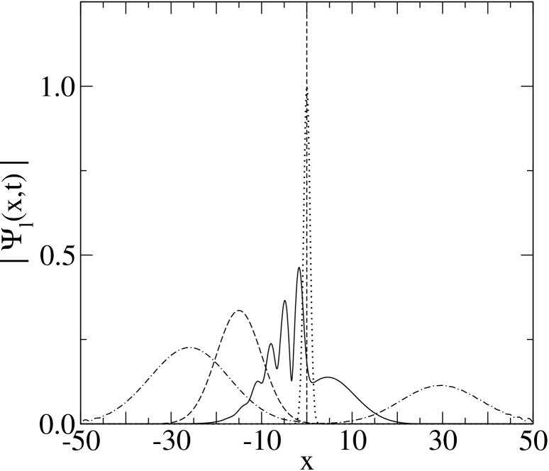
Figure 1: Modulus of the wave packet $|\Psi_{l}(x,t)|$ at times $t=0$ (dashed line), 18 (solid line), and 40 (dot-dashed line). The potential is portrayed by the dotted line.

$|\Psi_{l}(x,t)|$ of the wave packet is shown in Fig. 1 at times $t=0$, 18, and 40, for the momentum $K=1.06$. The potential is frozen in time with $v(t)=1$. The energy is 0.571834 which includes the zero point kinetic energy (0.01) and a small contribution from the potential energy (0.000034); the latter due to the overlap of the tails of the potential and initial wave packet. The energy of the colliding packet is slightly above half the barrier height.

The difference between the negative and positive sides of the packet at $t=18$ is most telling. The modulus for negative values of $x$ shows clearly the interference between the incoming and reflected waves while that on the positive-$x$ side exhibits a good fraction of the transmitted packet. At $t=40$ we clearly observe two distinct Gaussian packets corresponding to the reflected and transmitted waves. The shapes of the reflected and transmitted waves have been effectively restored to the original Gaussian shape, with no memory of the interaction with the potential.

In Fig. 2 the average position

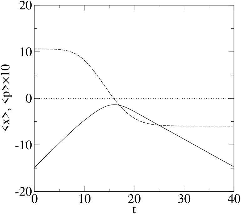
Figure 2: The average position (solid line) and average momentum (dashed line) of the wave packet as a function of time. The initial momentum is $K=1.06$. To facilitate the display, the momentum has been multiplied by a factor of 10.

$\left\langle x\right\rangle$ and average momentum $\left\langle p\right\rangle$ of the wave packet as a function of time are displayed as the solid and dashed lines respectively. At $t=0$, the packet center starts from $x=-3\lambda_{0}=-15$ with an initial momentum of $K=1.06$. The interaction with the barrier begins at $t\sim 12$ as denoted by the change in the momentum. The packet slows down and stops at $t\sim 15$ after which 80% of it is reflected. The final average momentum may be estimated to be $-0.64=-1.06\times 0.6$ due to the transmission of $\sim 20\%$ of the wave. This is comparable to the actual value of the momentum $\left\langle p\right\rangle=-0.60$ at $t=40$.

In seeking evidence for a resonance behavior under the barrier, we also investigated the behavior of the even and odd solutions of the TDSE. We show in Fig. 3 the absolute value of the even

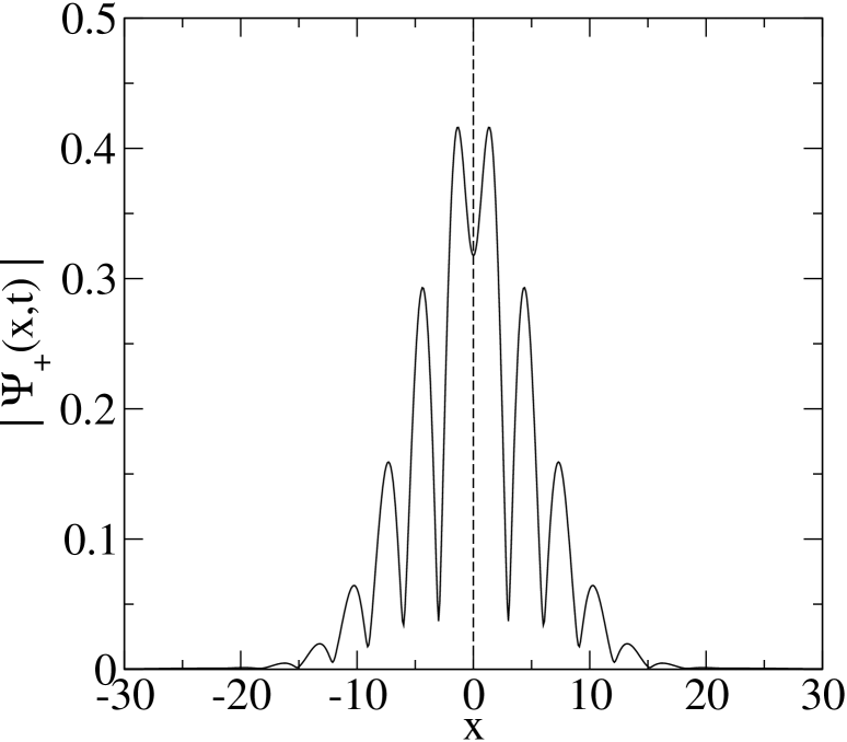
Figure 3: $\left|\Psi_{+}\right|$ at $t=15.75$ corresponding to maximal presence under the barrier.

solution $\Psi_{+}$ at $t=15.75$ and for $K=1.06$. Approximately these conditions correspond to the situation of maximum interaction with the barrier. Note there is no peak of $\left|\Psi_{l}\right|$ under the barrier, and $\Psi_{-}$ has a node at $x=0$. Therefore, we sought to create a “bump under the barrier” for some combination $\Psi_{\text{mix}}=\Psi_{+}\cos{\theta}+\Psi_{-}e^{i\varphi}\sin{\theta}$. The propagation of this mixed wave is then analyzed in classical terms of a bump position and momentum. We could not find any combination of $\theta$ and $\varphi$ giving such a bump. This stems from the strong positive curvature of $\Psi_{+}$ at $x=0$ while $\Psi_{-}$ has no curvature at its node. Hence, for any given $\theta$ both $\Psi_{\text{mix}}$ and its second derivative have the same sign at $x=0$. No bump can be found as such would require opposite signs.

We display in Figs. 4 to 9, the transmitted norm of the wave $\Psi_{l}$. The transmitted norm is defined as a function of time as

$$T(t)=\int_{5}^{\infty}\left|\Psi_{l}(x,t)\right|^{2}\;dx.$$ (6)

The lower bound in the integral, $x=5$, is chosen to be far enough away from the barrier to ensure no contamination of the transmitted wave by the barrier. We are also interested in the asymptotic value of the transmitted norm, $T(\infty)$. This observable is also important for comparisons of different potentials. Fig. 4 shows the case for the reference potential, $V(x)=e^{-x^{2}}$, with $K=1.06$.

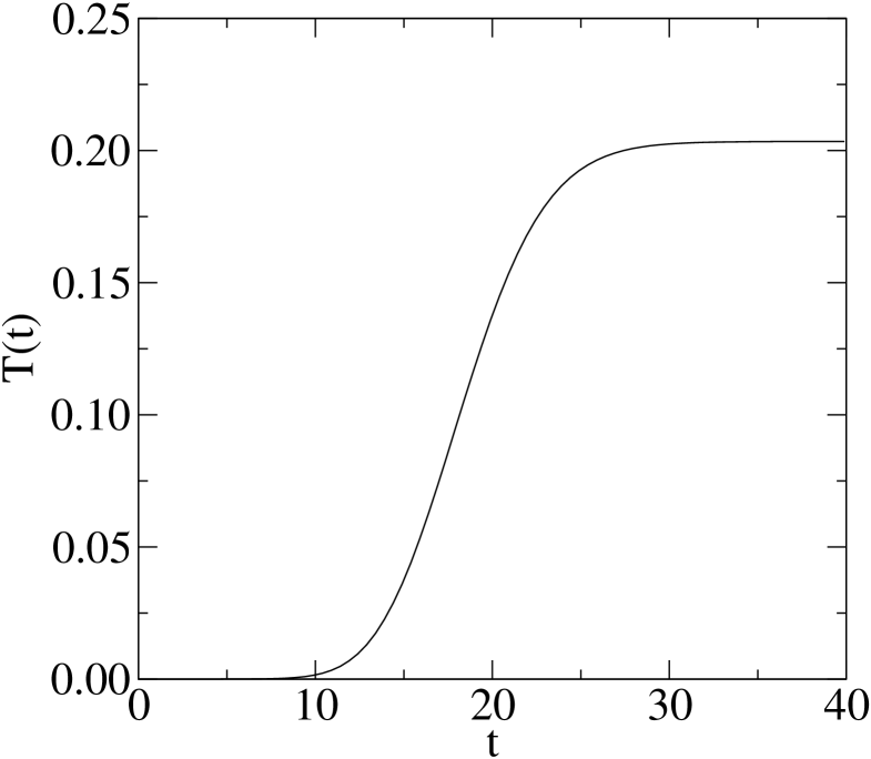
Figure 4: Transmitted norm $T(t)$ for the case $K=1.06$ and for the reference potential.

The asymptotic value for this case is $T(\infty)=0.203$ confirming the earlier observation of 20% transmission for the wave with $K=1.06$.

III Spatial variations of the potential

In this section, we investigate time-independent potentials which vary with respect to space. As we are discussing time-independent potentials, the time variable is omitted from the discussion for the moment.

Given the same starting wave packet as in Section II, transmission through a barrier $V_{1}(x)$ will be less than that through barrier $V_{2}(x)$ if $V_{1}(x)>V_{2}(x)$, $\forall x$. Details of the shape of the incident packet may change this result. But we assume packets to be close to eigenstates, for which theorems bounding growth and curvatures of waves in relation to the potential hold. To investigate deviations from this estimate, we compare results for potentials where $V_{1}(x)>V_{2}(x)$ for some $x$, and $V_{1}(x)<V_{2}(x)$ for other values.

This is achieved by using the following modulation to our base potential,

$$W(x)=\sigma e^{-2\omega x^{2}}\left[\sin{\left(11x\right)}\sin{\left(13\sqrt{2}x\right)}\cos{\left(2\pi x\right)}\cos{\left(\frac{5x}{\sqrt{2}}\right)}+\tau\sin{\left(3\sqrt{\pi}x\right)}\sin{\left(7x\right)}\right],$$ (7)

where $\sigma$ is the strength of the modulation and $\tau$, which is weakly dependent on $\sigma$, is used to cancel the semi-classical effect introduced by $W(x)$ (discussed below).

III.1 Problem of a fair comparison

To achieve a fair comparison to our base potential, we rely on the action integral

$$\mathcal{A}=\int_{x_{l}}^{x_{r}}dx\sqrt{2\left[E-V(x)-W(x)\right]}\;,$$ (8)

where $E$ is the energy of the packet and $x_{l}$ and $x_{r}$ are the left and right turning points respectively. Of course this assumes that there are only two such turning points. We compare potentials for which $\mathcal{A}$ is invariant. Fig. 5 shows three such potentials for $E=0.571834$.

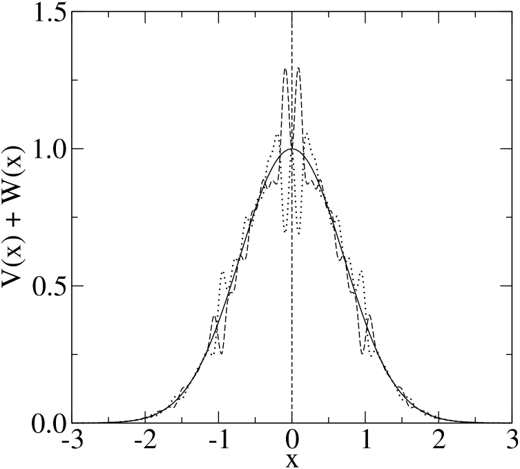
Figure 5: The potentials used for solving the TDSE. The base potential ($W(x)=0$) is given by the solid line, while the potentials for $\sigma=0.5$ (ears up) and $\sigma=-0.5$ (ears down) are given by the dashed and dotted lines respectively.

The base potential $V(x)$ is portrayed by the solid line. The modulations introduced by Eq. (7) correspond to the case $\sigma=0.5$, $\tau=-0.111$ (dashed line, “ears up”) and $\sigma=-0.5$, $\tau=-0.132$ (dotted line, “ears down”). The slight difference in the value of $\tau$ comes from the condition of satisfying the semi-classical action specified in Eq. (8). If one requires that the average modulations vanish, i.e. $\mathcal{W}=\int^{\infty}_{-\infty}W(x)dx=0$, then $\tau=-0.118$; a value not too different from the two values given. In fact, for $\tau=-0.111$, $\mathcal{W}=8\times 10^{-4}$, while for $\tau=-0.132$, $\mathcal{W}=2\times 10^{-3}$. Thus the modulations we have introduced do not change the semi-classical action and the associated changes in the average of the potential are negligible.

III.2 Results

In Fig. 6, we display the transmitted norm $T(t)$ for the three potentials described and for an incident wave packet with $K=1.06$.

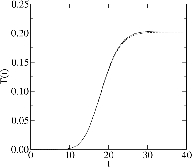
Figure 6: Transmitted norms for a wave packet with $K=1.06$ incident on the three potentials. The curves correspond to the results obtained for the reference (solid line), “ears up” (dashed line), and “ears down” (dotted line) potentials.

Transmission is hardly affected by the changes to the reference potential. For the “ears up” potential $T(40)=0.202$ while for the “ears down” it is 0.204. These are to be compared with the value of 0.203 found using the reference potential. These changes, of the order of a percent, are small in comparison to the associated variations of the potentials from the reference; the modulations of which are as much as 30%. That is especially so in the region of the “ears”.

Results have been obtained also for the same potentials but with lower incident momenta. For $K=0.6$, hence $E=0.190034$, the condition of fair comparison [Eq. (8)] of potentials with modulations defined by Eq. (7) requires $\tau=0.050$ for $\sigma=0.5$ and $\tau=-0.084$ for $\sigma=-0.5$. These parameters give also the “ears up” and “ears down” potentials respectively with fluctuations on reference $\sim\pm 30\%$ in the ears. The results for the transmitted norm in this case are displayed in Fig. 7.

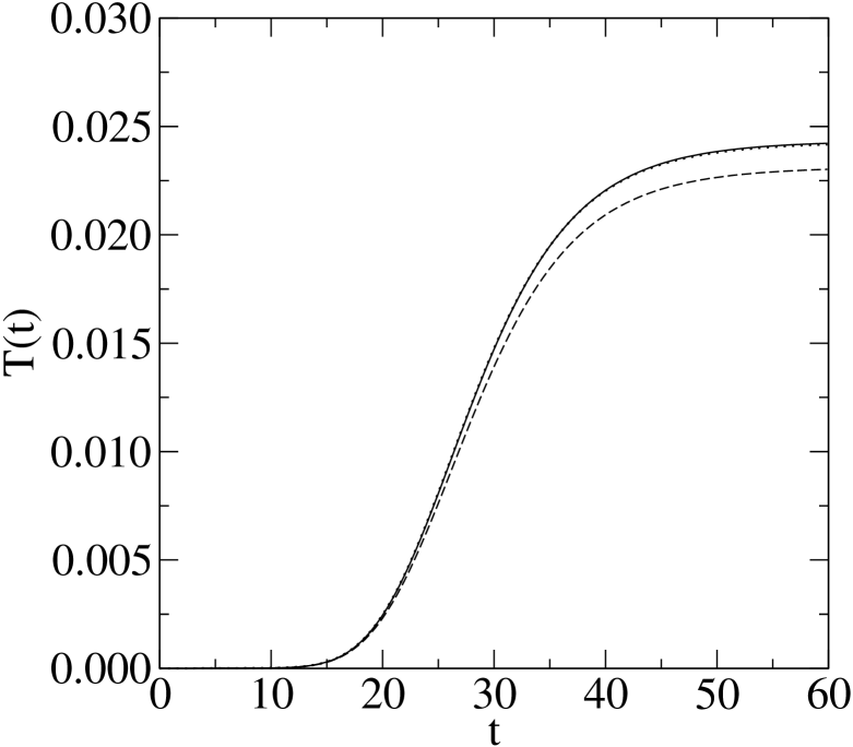
Figure 7: As for Fig. 6 but for $K=0.6$.

For the “ears-up” potentials at this energy, the transmission now appears depleted as the value of $T(\infty)$ in this case is 0.0226. But there is little change for the “ears-down” case from the asymptotic transmitted norm obtained for the reference potential, 0.0239.

A different picture occurs for the case $K=0.42$, or $E=0.098234$. This is displayed in Fig. 8 for the same potentials used previously.

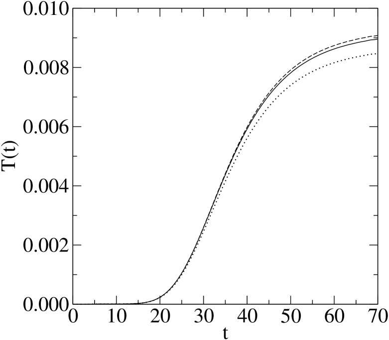
Figure 8: As for Fig. 6 but for $K=0.42$.

For the lowest momentum considered, there is a slight enhancement in the transmission from the “ears-up” potential and a significant depletion with the “ears-down” potential. This is the reverse situation to that with $K=0.6$.

The modulating potential $W(x)$ in [Eq. (7)] is not the only form that we have considered. Another is

$$W(x)=\sigma e^{-2\omega x^{2}}\left[\sin{\left(17x\right)}\sin{\left(13\sqrt{2}x\right)}\cos{\left(\frac{11x}{\sqrt{2}}\right)}\cos{\left(7\pi x\right)}+\tau\sin{\left(3\sqrt{\pi}x\right)}\sin{\left(7x\right)}\right].$$ (9)

The results for the transmitted norm with this modulation are displayed in Fig. 9 for $K=0.46$, $\sigma=\pm 0.5$ and $\tau=0.141$ and $0.028$, respectively for the sign of $\sigma$. While there

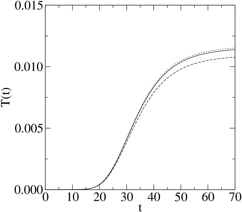
Figure 9: As for Fig. 6 but for $K=0.46$ and with the modulating potential $W(x)$ given by Eq. (9).

appears to be little change in transmission with the “ears-down” potential there is some depletion with the “ears-up” case.

It is noteworthy that, with any of these modifications to the reference potential, the effect on the transmission is minimal; changes being at most of the order of 10%. This is not sufficient to explain the observed depletion of fusion rates below the Coulomb barrier.

IV Fluctuations in time

As the spatial fluctuations are unlikely to be the source of the large loss of fusion that is observed experimentally, we turn our attention to time-dependent fluctuations on the base potential. We assume those fluctuations are of the form

$$v(t)=1+\gamma\cos{\left(\Omega_{c}t\right)}\sin{\left(\Omega_{s}t\right)}.$$ (10)

We take $\gamma=0.2$ while $\Omega_{c}$ and $\Omega_{s}$ are chosen at random with uniform distributions varying between 0 and 5 for $\Omega_{c}$ and between $-5$ and 5 for $\Omega_{s}$. These parameters are then sampled allowing for a good simulation of the chaotic character of $(v(t)-1)$.

We start again with our initial wave packet, Eq. (4). The fine structures in the packet experience the weakly correlated components of the oscillating fluctuations and so we need not be concerned about any time periodicity in $V(x,t)$. The sampling space is one of 200 to 500 potentials (independent choices for $\Omega_{c}$ and $\Omega_{s}$) and we use the asymptotic value of the transmitted norm $T(\infty)$ as the measure of effect of the time-dependent potentials in comparison to that from the reference potential for which $v(t)=1$. The latter we designate as $T_{R}(\infty)$.

Displayed in Fig. 10 is the ratio of $T(\infty)/T_{R}(\infty)$, obtained from 200 runs for a packet with initial momentum $K=0.6$.

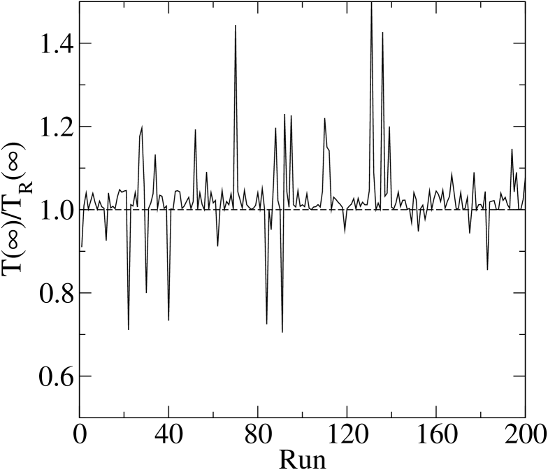
Figure 10: Ratio of $T(\infty)$ against the reference value ($T_{R}(\infty)=0.0239$) for the runs made using the random pair of $\left\{\Omega_{c},\Omega_{s}\right\}$ specified in Eq. (10). For these calculations, $K=0.6$. The line is a guide to the eye.

The reference value for this case is $T_{R}(\infty)=0.0239$. For most of the pairs sampled, the transmission is close to the reference potential. But there are a few instances where the tunneling is greatly enhanced as well as others where it is greatly reduced. Variations of as much as 50% occur. The distribution of values of $T(\infty)$ for $K=0.6$ is displayed in Fig. 11.

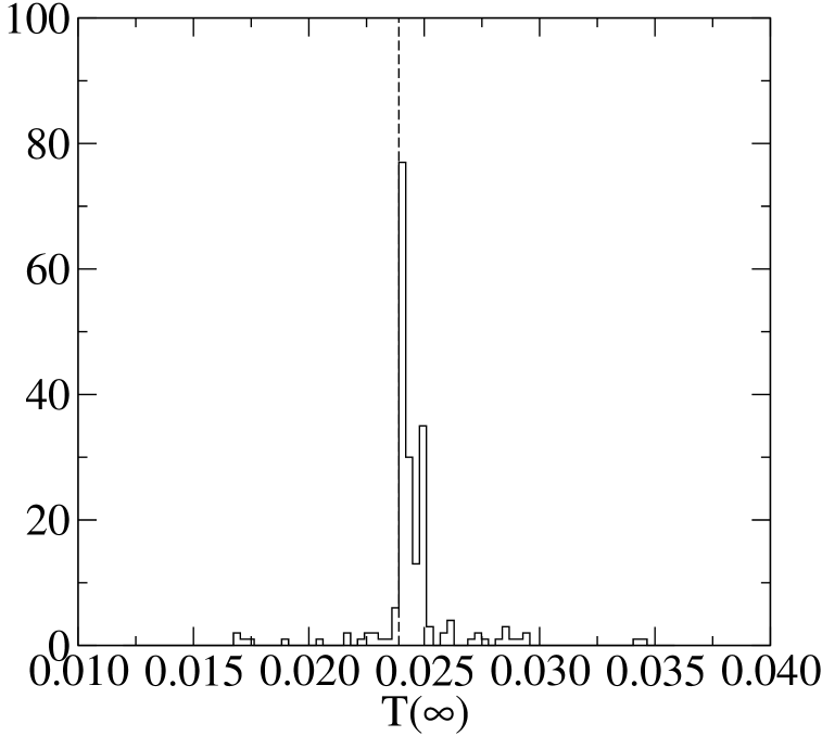
Figure 11: Distribution of values of $T(\infty)$ for the runs shown in Fig. 10, for which $K=0.6$. The reference value $T_{R}(\infty)=0.0239$ is indicated by the dashed line.

As indicated in Fig. 10, the introduction of time fluctuating potentials increases slightly the value of $T(\infty)$ on average indicating that the transmission is enhanced, if only a little. That is a general feature we find for many conditions and one such is shown in Fig. 12. Therein the histogram for runs with

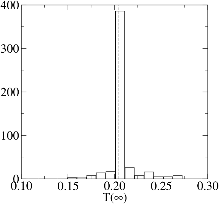
Figure 12: As for Fig. 11 but for $K=1.06$ and using a sample of 500 potentials. The value of $T_{R}(\infty)$ for the reference potential is 0.2039.

$K=1.06$ (sample size of 500) are displayed. The slight increase of $T(\infty)$ on average is evident again.

V 3-dimensional model

V.1 Formalism for a more realistic model

We now consider 3-dimensional eigenstates of the Hamiltonian $H=-\partial^{2}/(2\partial r^{2})+V_{\text{sqC}}(r)$, where $V_{\text{sqC}}(r)$ is an approximation to the central radial potential for a realistic nucleus. The potential is built using a series of square wells to approximate an attractive nuclear potential plus a Coulomb barrier. In our dimensionless units, the nuclear part is taken as a square well with depth $U=-2$ with range $R=2$ while the Coulomb interaction is approximated by a staircase with 20 steps between $r=2$ and $r=10$, with no repulsion beyond $r=10$. The center of the $n^{\text{th}}$ step is $r_{n}=2.2+0.4(n-1)$ and so to construct a Coulomb barrier with strength 3 in our units, the height of the $n^{\text{th}}$ step is $3/r_{n}$. The potential is shown in Fig. 13.

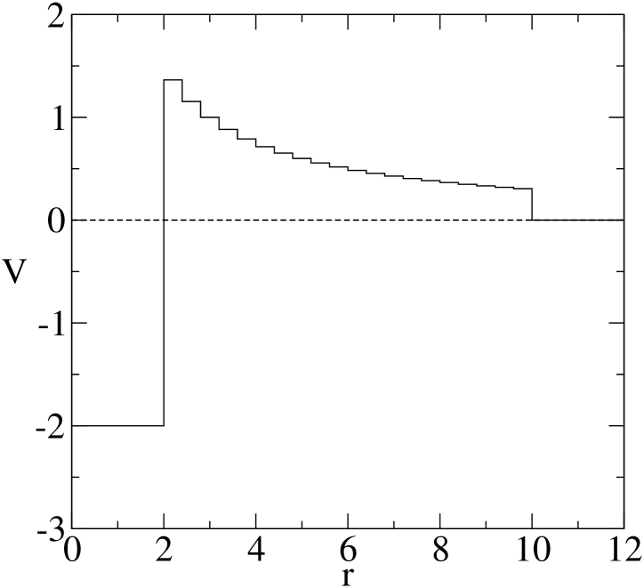
Figure 13: The radial potential $V_{\text{sqC}}(r)$ in the 3D problem.

We shall consider tunneling using this potential for energies in the range $0.1<E<0.7$, equating roughly from a third of the outermost step to the height of the middle (sixth) step, i.e. about half the maximum barrier. This choice is dictated by a need to study sub-Coulomb processes as well as a need to minimize effects of discontinuities arising from the highest steps in the staircase. Also we consider $s$-wave scattering only as this simplifies calculations using square wells. For a given incident momentum $K$ and energy $E=K^{2}/2$, the momentum inside the potential is $k=\sqrt{K^{2}-2U}$. We normalize the solution by a unit derivative for the innermost part of the wave, namely $\sin{(kr)}/k$, so that we can define the square norm for “presence in the attractive well” as $\mathcal{N}=R/(2k^{2})-\sin{(2kR)}/(4k^{3})$. With the incident wave function given by

$$\Psi=A\left[e^{-iKr}+Be^{iKr}\right],$$ (11)

matching the wave function and its logarithmic derivative at each step boundary gives the parameters $A$ and $B$. At each energy, the test for unitarity, $\left|B\right|=1$, is made to check numerical accuracy.

The relevant measure we define as the transmission index; a quantity given by $\mathcal{T}=\mathcal{N}/\left|A\right|$. This one can view as an “inside square norm per unit (incoming) flux”. For a given energy $E$, it is also possible to find both outer and inner turning points, and the corresponding classical action [Eq. (8)].

V.2 Results

Solution of the tunneling problem with the 3-D staircase potential give the classical action displayed in Fig. 14 as a function of $E$.

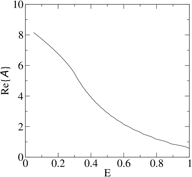
Figure 14: Energy variation of the reference classical action for tunneling under the potential $V_{\text{sqC}(r)}$.

While the discontinuities in the staircase potential make the derivative of $\mathcal{A}$ discontinuous, $\mathcal{A}$ itself is continuous and the derivative does not jump significantly. It is expected that $\ln{\mathcal{T}}$ will be roughly proportional to $\mathcal{A}$. This is confirmed in Fig. 15, which shows the ratio of $\ln{\mathcal{T}}$ to $\mathcal{A}$ as a function of $E$.

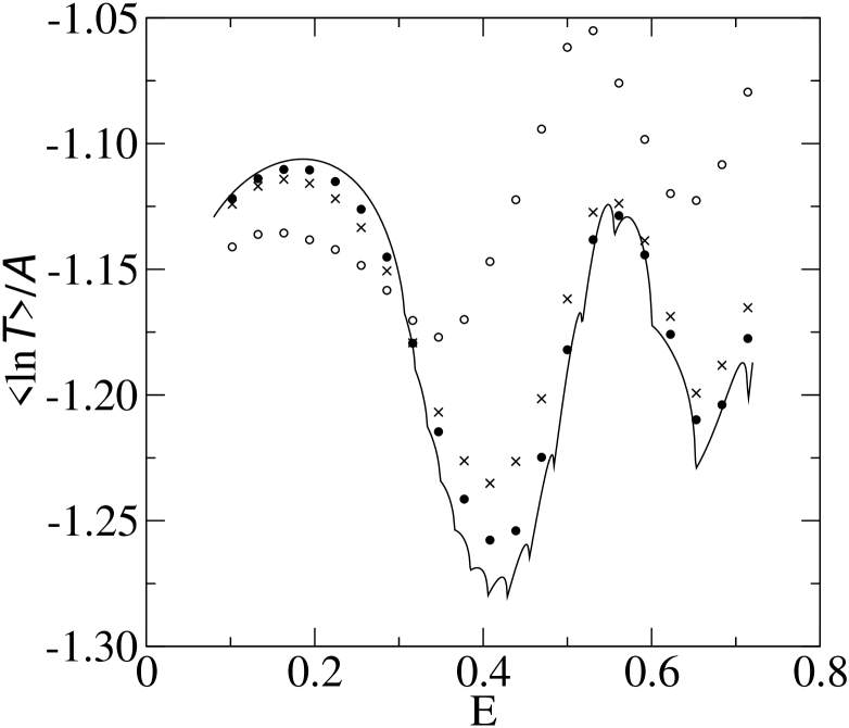
Figure 15: Ratio $\left\langle\ln{\mathcal{T}}\right\rangle/\mathcal{A}$ as a function of energy. The solid curve was obtained by using the reference potential $V_{\text{sqC}}$. The closed circles depict the result found by using a fluctuation energy of 0.0929 while the open circles correspond to use of an energy 3 times greater. The crosses are the results found on using a fluctuation set at 10% of the highest strength value.

Despite oscillations and a fine structure, the latter due to the discontinuities in the staircase potential approximating the Coulomb interaction, an average value for the ratio of $-1.2$ to within a few percent is observed for all of the calculations made, including fluctuations that are described next.

To incorporate fluctuations we introduce a random modification $w_{n}$ of the $n^{\text{th}}$ step which raises or lowers the height of that step. The sampling is from a uniform distribution with typically

$$\frac{3}{r_{5}}-\frac{3}{r_{4}}<w_{n}<\frac{3}{r_{4}}-\frac{3}{r_{5}}\text{ where }\frac{3}{r_{4}}-\frac{3}{r_{5}}=0.0929\,.$$ (12)

We also allow for an increase or a decrease of this range by some factor. But introducing such fluctuations no longer guarantees that the staircase potential will be monotonic and it may allow for the propagation of the wave at positive local energies above a few intermediate steps. This will give more than two turning points although the number will always be even.

We must also consider the fairness criterion of Eq. (8) when invoking fluctuations. We do this for each perturbed staircase potential $V_{p}$ by calculating the classical action $\mathcal{A}^{\prime}$, taking into account the possibility of the existence of more than two turning points because of the (possible) presence of local minima. We compare $\mathcal{A}^{\prime}$ to that ($\mathcal{A}$) of the reference staircase potential and reject any $V_{p}$ from our sample if $|\mathcal{A}^{\prime}/\mathcal{A}-1|>10^{-4}$. As a check, we verify that our results do not depend on any variation in the tolerance. Finally, we average $\ln{\mathcal{T}}$ over the subset of perturbed potentials that meet the selection criterion.

For each energy $E$, we sample between $10^{5}$ and $10^{6}$ staircase potentials in the fluctuation space. However, the fairness criterion is severe: only a few thousand, or even a few hundred, staircase potentials are retained. The acceptance rate, an increasing function of the tolerance as well as a decreasing function of the range of fluctuations, also is a decreasing function of the energy. Typically, the number of accepted potentials is five times smaller for $E=0.7$ than it is for $E=0.1$. Possibly that is due to the local momenta $k=\sqrt{2\left[E-V_{p}(r)\right]}\to 0$ with a larger derivative as $E$ increases, which in turn would lead to a larger variation in the classical action. Note also, that for such numbers of accepted potentials, we also verify that the average of the logarithm of the transmission index $\left\langle\ln{\mathcal{T}}\right\rangle$ barely differs from the logarithm of the average transmission $\ln{\left\langle\mathcal{T}\right\rangle}$. A typical result is shown in Fig. 15 where the dots correspond to the fluctuation range 0.0929 and the open circles to one that is three times larger. An interesting phenomenon is that fluctuations decrease the transmission at lower energies while they increase it at higher energies. The transition between these two regimes occurs near $E\sim 0.3$. But this would not seem to be a significant reason for the depletion or enhancement of tunneling, as long as the fluctuations do not exceed 10% of the potential. That result corresponds to the crosses in Fig. 15. We verified this result numerically also for other parameter sets within the model. It may be concluded that within our present understanding of friction, the lower than expected fusion cross sections cannot be explained by the processes discussed either with the 1D or the 3D models.

VI Discussion and conclusions

We have considered various cases of tunneling in a fully quantal approach, changing the base potential in our model by adding either space-dependent or time-dependent fluctuations to see if there is any enhancement in the transmission of the packet beyond the barrier. For the cases of the space-dependent fluctuations, the induced changes were made such that the classical action was invariant so allowing for a fair comparison of the results obtained with those of the base (reference) potential. The effects of those changes seem to be momentum dependent. For a high incident momentum, corresponding to $K=1.06$, there is very little change in the transmission of the wave through the barrier. For much lower momenta, particularly the case for $K=0.42$, there is change, with the “ears up” potential producing a reduction in the transmission. The same occurs at this momentum for an effectively random change in the modulating potential. But the size of the changes in the transmission are not very large, typically $\sim 10\%$ and given that we can produce both enhancement and depletion by such (relatively large) changes in the barrier, we conclude that the cause of the large ($\sim 50\%$) loss of fusion observed experimentally is unlikely to be solely, or even largely, caused by changes in the transmission due to space fluctuations in the barrier.

By perturbing the barrier with time-dependent oscillations, we have been able to produce a small systematic increase in the transmission. Yet with our sample over a large number of potentials and at various incident momenta we were only able to find small numbers of cases where the transmission was either greatly enhanced or greatly diminished. The enhancement may correspond to a situation where fusion is also enhanced and vice-versa. However, the number of such cases is relatively few, and the average of all lead to small enhancements in transmission for all momenta.

We also considered a more realistic three-dimensional case using a potential made up of a series of square wells approximating the nuclear plus Coulomb potentials of the nucleus. This allowed us to treat the problem analytically and so consider the effect of transmission more closely. Again we allowed some fluctuations into the system, this time by small perturbations to the square wells constructing the Coulomb barrier. As with the one-dimensional cases, we observed only small changes to the results of transmission obtained for the reference radial potential. There were no significant changes that might produce the observed lack of fusion.

In all cases, there is one overriding consideration: there is no evidence for a “friction” related to a Langevin process with complex time. By considering the full quantal TDSE no such effects with classical analogues, or those involving complex time, are needed to produce changes to the observed transmission. But those changes are not significant enough to indicate that the source of the depletion of fusion rates in heavy-ion reactions at extreme sub-Coulomb barrier energies comes from changes in tunneling.