Consequences of wall stiffness for a $\beta$-soft potential

Abstract

Modifications of the infinite square well E(5) and X(5) descriptions of transitional nuclear structure are considered. The eigenproblem for a potential with linear sloped walls is solved. The consequences of the introduction of sloped walls and of a quadratic transition operator are investigated.

I Introduction

The E(5) and X(5) models have been proposed by Iachello iachello2000:e5 ; iachello2001:x5 to describe the essential characteristics of shape-transitional forms of quadrupole collective structure in nuclei. The E(5) model, for $\gamma$-soft nuclei, and the X(5) model, for axially symmetric nuclei, are both based upon the approximation of the potential energy as a square well in the Bohr deformation variable $\beta$. These models produce predictions for level energy spacings and electromagnetic transition strengths intermediate between those for spherical oscillator structure and for deformed $\gamma$-soft wilets1956:oscillations or deformed axially-symmetric rotor bohr1998:v2 structures.

The X(5) predictions for level energy spacings and electromagnetic transition strengths have been extensively compared with data for nuclei in transitional regions between spherical and rotor structure casten2001:152sm-x5 ; bizzeti2002:104mo-x5 ; kruecken2002:150nd-rdm ; brenner2002:x5-a80a100 ; caprio2002:156dy-beta ; hutter2003:104mo106mo-rdm ; clark2003:x5-search ; mccutchan2004:162yb-beta ; bijker2003:x5-gamma . For several such nuclei, including the $N$=90 isotopes of Nd, Sm, Gd, and Dy, the X(5) predictions match well the yrast band level energies and the excitation energy of the $K^{\pi}$$=$$0^{+}_{2}$ band head [Fig. 1(a,b)]. The X(5) predictions also reproduce essential features of the electric quadrupole transitions from the $K^{\pi}$$=$$0^{+}_{2}$ band to the ground state band: the presence of strong spin-ascending interband transitions but highly-suppressed spin-descending transitions.

Figure 1: Evolution of the (a) $4^{+}_{1}$ energy, (b) $0^{+}_{2}$ energy, and (c) energy spacing scale of the excited $0^{+}$ sequence, all normalized to the $2^{+}_{1}$ energy, across the $N$=90 transition region, for the Nd (

$\square$

), Sm ( $\circ$ ), Gd (

$\vartriangle$

), and Dy (

$\blacksquare$

) isotopic chains. Shown for comparison are the X(5) predictions (solid line) and the present sloped well predictions for various values of the parameter $S$ defined in (12) — $S$$=$100 (long-dashed line), $S$$=$50 (short-dashed line), and $S$$=$25 (dotted line). Data are from Refs. nds1995:150 ; nds1996:152 ; nds1998:154 ; ndsboth:156 . (Figure based upon Ref. caprio2002:156dy-beta .)

However, several discrepancies exist between the X(5) predictions and observed values. The spacing of level energies in the $K^{\pi}$$=$$0^{+}_{2}$ band is predicted to be much larger than in the ground state band, but empirically at most a slightly larger energy scale is found for the $K^{\pi}$$=$$0^{+}_{2}$ band [Fig. 1(c)] caprio2002:156dy-beta ; clark2003:x5-search ; mccutchan2004:162yb-beta . This overprediction is encountered in descriptions of transitional nuclei with the interacting boson model (IBM) and geometric collective model (GCM) as well scholten1978:ibm-fits ; zhang1999:152sm-gcm . For nuclei with yrast band level energies matching the X(5) predictions, the yrast band $B(E2)$ strengths tend to fall below the X(5) predictions, and sometimes even below the pure rotor predictions (see Fig. 2 of Ref. clark2003:x5-search ). For the $N$=90 nuclei, the transitions between the $K^{\pi}$$=$$0^{+}_{2}$ and ground state bands have strength ratios typically matching those predicted, but their strength scale is considerably weaker than predicted casten2001:152sm-x5 ; kruecken2002:150nd-rdm ; caprio2002:156dy-beta ; clark2003:n90-x5 ; casten2003:n90-x5-comment .

It is thus necessary to ascertain which aspects of the X(5) description are most important in determining the predictions for these basic observables. The square well potential involves an infinitely-steep “wall” in the potential as a function of $\beta$, presumably a radical approximation. Moreover, the model has so far been used only with a first-order electric quadrupole transition operator, but the likely importance of second-order effects has been noted by Arias arias2001:134ba-e5 and by Pietralla and Gorbachenko pietrallaXXXX:beta-soft . In the present work, the infinitely stiff confining wall is replaced with a gentler, sloped wall, constructed using a linear potential. The effects upon calculated observables of the introduction of a sloped wall and of a quadratic transition operator are addressed. A computer code for solution of the sloped well eigenproblem is provided through the Electronic Physics Auxiliary Publication Service swell-epaps .

II Solution method

Consider the Bohr Hamiltonian bohr1998:v2

$$H=-\frac{\hbar^{2}}{2B}\Biggl{[}\frac{1}{\beta^{4}}\frac{\partial}{\partial\beta}\beta^{4}\frac{\partial}{\partial\beta}+\frac{1}{\beta^{2}\sin 3\gamma}\frac{\partial}{\partial\gamma}\sin 3\gamma\frac{\partial}{\partial\gamma}\\ -\frac{1}{4\beta^{2}}\sum_{\kappa}\frac{M_{\kappa}^{2}}{\sin^{2}(\gamma-\frac{2}{3}\pi\kappa)}\Biggr{]}+V(\beta,\gamma),$$ (1)

where $\beta$ and $\gamma$ are the Bohr deformation variables and the $M_{\kappa}$ are angular momentum operators, with potential

$$V(\beta)=\begin{cases}0&\beta\leq\beta_{w}\\ C(\beta-\beta_{w})&\beta>\beta_{w}.\end{cases}$$ (2)

Since this potential is a function of $\beta$ only, the five-dimensional analogue of the central force problem arises. The usual separation of “radial” ($\beta$) and “angular” variables wilets1956:oscillations ; rakavy1957:gsoft occurs, yielding eigenfunctions of the form $\Psi(\beta,\gamma,\omega)$$=$$f(\beta)\Phi(\gamma,\omega)$, where $\omega$$\equiv$$(\vartheta_{1},\vartheta_{2},\vartheta_{3})$ are the Euler angles. The angular wave functions $\Phi(\gamma,\omega)$, common to all $\gamma$-independent problems, are known bes1959:gamma . For the radial problem, following Rakavy rakavy1957:gsoft , it is most convenient to work with the “auxiliary” radial wave function $\varphi(\beta)$$\equiv$$\beta^{2}f(\beta)$. This function obeys a one-dimensional Schrödinger equation with a “centrifugal” term,

$$\left[-\frac{\hbar^{2}}{2B}\frac{\partial^{2}}{\partial\beta^{2}}+\frac{\hbar^{2}}{2B}\frac{\alpha}{\beta^{2}}+V(\beta)-E\right]\varphi(\beta)=0,$$ (3)

where the centrifugal coefficient $\alpha$ is related to the O(5) separation constant $\tau$ ($\tau$$=$$0,1,\ldots$) by $\alpha$$=$$(\tau+1)(\tau+2)$. For problems with a more general potential $V(\beta,\gamma)$$=$$V_{\beta}(\beta)+V_{\gamma}(\gamma)$, Iachello iachello2001:x5 showed that an approximate separation of variables occurs, provided that $V_{\gamma}(\gamma)$ confines the nucleus to $\gamma$$\approx$$0$ (see Ref. iachello2001:x5 for details). In this “$\gamma$-stabilized” case, the eigenfunctions are of the form $\Psi(\beta,\gamma,\omega)$$\propto$$f(\beta)\eta(\gamma)\phi_{KLM}(\omega)$, where the $\phi_{KLM}(\omega)$ are the conventional rigid rotor angular wave functions bohr1998:v2 for angular momentum $L$, $z$-axis projection $M$, and symmetry axis projection $K$. The auxiliary radial wave function again obeys (3), but now with $\alpha$$=$$\frac{1}{3}L(L+1)+2$.

In the region $\beta$$<$$\beta_{w}$, the potential $V(\beta)$ of (2) vanishes, and the radial equation (3) reduces to the Bessel equation of order $\nu$$=$$(\alpha+1/4)^{1/2}$. The solutions with the correct convergence properties at the origin are $\varphi(\beta)$$\propto$$\beta^{1/2}J_{\nu}(\varepsilon^{1/2}\beta)$, where $\varepsilon$$\equiv$$(2B/\hbar^{2})E$. In the region $\beta$$>$$\beta_{w}$, where the potential is linear in $\beta$, an analytic solution does not exist for the full problem with centrifugal term. For $\alpha$$=$$0$ only, (3) reduces to the Airy equation, with solutions $\varphi(\beta)$$\propto$$\mathrm{Ai}[c^{1/3}(\beta-\beta_{w})-c^{-2/3}\varepsilon]$, where $c$$\equiv$$(2B/\hbar^{2})C$.

The analytic solutions obtained for $\alpha$$=$$0$ provide a very efficient basis for numerical diagonalization to obtain the true $\alpha$$\neq$$0$ solutions of the radial equation (3). It is first necessary to obtain a basis set of $\alpha$$=$$0$ solutions

$$\varphi_{i}^{\alpha=0}(\beta)=\begin{cases}N_{1}\beta^{1/2}J_{1/2}[(\varepsilon_{i}^{\alpha=0})^{1/2}\beta]&\beta\leq\beta_{w}\\ N_{2}\mathrm{Ai}[c^{1/3}(\beta-\beta_{w})-c^{-2/3}\varepsilon_{i}^{\alpha=0}]&\beta>\beta_{w}.\end{cases}$$ (4)

The eigenvalues of $\varepsilon$ are determined by the condition that $\varphi(\beta)$ be continuous and smooth at the matching point $\beta$$=$$\beta_{w}$. This yields a transcendental equation which is solved numerically for $\varepsilon$. The normalization coefficients $N_{1}$ and $N_{2}$ then follow from continuity and the requirement $\int_{0}^{\infty}d\beta|\varphi(\beta)|^{2}$$=$$1$. Since the radial equation (3) has the form of a one-dimensional Schrödinger equation, its solution for general values of $\alpha$ may be carried out as the matrix diagonalization problem for a corresponding “Hamiltonian” matrix $h$, including the centrifugal potential, with respect to these $\alpha$$=$$0$ basis functions, with entries

$$h_{ij}\equiv\delta_{i,j}\varepsilon_{i}^{\alpha=0}+\alpha\int_{0}^{\infty}d\beta\,\varphi_{i}^{\alpha=0}(\beta)\,\frac{1}{\beta^{2}}\,\varphi_{j}^{\alpha=0}(\beta).$$ (5)

Convergence in this basis is rapid — for instance, the eigenvalues of the ground state and first excited radial solution converge to within $\sim$$1.5\%$ of their true values with a truncated basis of only $5$ eigenfunctions. Values shown in this paper are calculated for a basis size of 25. For illustration, an example potential, with centrifugal contribution, and the corresponding calculated eigenvalues are shown in Fig. 2.

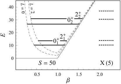
Figure 2: Energies of low-lying $0^{+}$ and $2^{+}$ levels for the sloped well potential with $S$=50. The potential without the five-dimensional centrifugal term is shown (solid curve), together with the potential including the centrifugal contributions for $L$$=$$0$ and $L$$=$$2$ (dashed curves). The energies of the corresponding states for the X(5) model are shown for comparison at right. [The $S$$=$$50$ calculation is for $2B/\hbar^{2}$$=$$1$ and $\beta_{w}$$=$$1$, while the X(5) calculation is scaled to $\beta_{w}$$=$$1.40$ to provide the same ground state eigenvalue.]

Electromagnetic transition strengths can be calculated from the matrix elements of the collective multipole operators. The general $E2$ operator for the geometric model gneuss1971:gcm ; hess1981:gcm-pt-os-w ; eisenberg1987:v1 may be expanded in laboratory frame coordinates $\alpha_{2\mu}$ as endnote-e2conjugate

$$\mathfrak{M}(E2;\mu)=A_{1}\alpha_{2\mu}+A_{2}[\alpha\times\alpha]^{(2)}_{\mu}+\cdots.$$ (6)

For the present purposes, it is necessary to reexpress this operator in terms of the intrinsic frame coordinates and $D^{2}(\omega)$ endnote-dfunction , giving, to second order in $\beta$,

$$\mathfrak{M}(E2;\mu)=A_{1}\beta\bigl{[}D^{2\,*}_{\mu 0}\cos\gamma+\frac{1}{\sqrt{2}}(D^{2\,*}_{\mu 2}+D^{2\,*}_{\mu-2})\sin\gamma\bigr{]}\\ -\sqrt{\frac{2}{7}}A_{2}\beta^{2}\bigl{[}D^{2\,*}_{\mu 0}\cos 2\gamma-\frac{1}{\sqrt{2}}(D^{2\,*}_{\mu 2}+D^{2\,*}_{\mu-2})\sin 2\gamma\bigr{]}.$$ (7)

In both the $\gamma$-independent and $\gamma$-stabilized cases, the matrix element of $\mathfrak{M}(E2;\mu)$ between two eigenstates factors into an angular integral and a radial integral. Here we consider matrix elements between unsymmetrized $\gamma$-stabilized wave functions bohr1998:v2

$$\Psi_{\alpha KJM}=\left(\frac{2J+1}{8\pi^{2}}\right)^{1/2}D^{J\,*}_{MK}(\omega)\,\Phi_{\alpha KJ}(\beta,\gamma),$$ (8)

as needed in calculations for the rigid rotor, X(5), or $\gamma$-stabilized sloped well models. The matrix element separates into intrinsic and Euler angle integrals, yielding

$$\left\langle\Psi_{\alpha^{\prime}K^{\prime}J^{\prime}M^{\prime}}||\mathfrak{M}(E2;\mu)||\Psi_{\alpha KJM}\right\rangle=\\ (-)^{J^{\prime}-J}(J^{\prime}K^{\prime}2(K-K^{\prime})|JK)\left[A_{1}I_{1}-\sqrt{\frac{2}{7}}A_{2}I_{2}\right],$$ (9)

in terms of

$$I_{1} \equiv\int d\tau\,\Phi_{\alpha^{\prime}K^{\prime}J^{\prime}}^{*}(\beta,\gamma)\,\beta\cos\gamma\,\Phi_{\alpha KJ}(\beta,\gamma)$$ (10)

$$I_{2} \equiv\int d\tau\,\Phi_{\alpha^{\prime}K^{\prime}J^{\prime}}^{*}(\beta,\gamma)\,\beta^{2}\cos 2\gamma\,\Phi_{\alpha KJ}(\beta,\gamma)$$

for $K^{\prime}$$-$$K$$=$$0$ or

$$I_{1} \equiv\int d\tau\,\Phi_{\alpha^{\prime}K^{\prime}J^{\prime}}^{*}(\beta,\gamma)\,\frac{1}{\sqrt{2}}\beta\sin\gamma\,\Phi_{\alpha KJ}(\beta,\gamma)$$ (11)

$$I_{2} \equiv\int d\tau\,\Phi_{\alpha^{\prime}K^{\prime}J^{\prime}}^{*}(\beta,\gamma)\,(-)\frac{1}{\sqrt{2}}\beta^{2}\sin 2\gamma\,\Phi_{\alpha KJ}(\beta,\gamma),$$

for $K^{\prime}$$-$$K$$=$$\pm 2$, where $d\tau$$\equiv$$\beta^{4}d\beta\left|\sin 3\gamma\right|d\gamma$ and the reduced matrix element normalization convention is that of Rose rose1957:am . (The matrix elements of the symmetrized wave functions, for $K$$\neq$$0$, may be calculated from this matrix element as usual bohr1998:v2 .) Considering the present $\beta$-$\gamma$ separated wave functions $\Phi(\beta,\gamma)$$=$$f(\beta)\eta(\gamma)$, for the case of no $\gamma$ excitation (so $K^{\prime}$$=$$K$$=$$0$), and under the approximation $\gamma$$\approx$$0$, these integrals reduce to $I_{1}$$=$$\int\beta^{4}d\beta f_{\alpha^{\prime}K^{\prime}J^{\prime}}(\beta)\beta f_{\alpha KJ}(\beta)$ and $I_{2}$$=$$\int\beta^{4}d\beta f_{\alpha^{\prime}K^{\prime}J^{\prime}}(\beta)\beta^{2}f_{\alpha KJ}(\beta)$. Transition strengths are $B(E2;J$$\rightarrow$$J^{\prime})$$=$$\linebreak[0](2J^{\prime}+1)\linebreak[0]/(2J+1)\linebreak[0]\,|\left<J^{\prime}||\mathfrak{M}(E2)||J\right>|^{2}$. Quadrupole moments, defined by $eQ_{J}$$\equiv$$(16\pi/5)^{1/2}\linebreak[0]\,\langle JJ|\mathfrak{M}(E2;0)|JJ\rangle$, may be calculated as $eQ_{J}$$=$$(16\pi/5)^{1/2}\linebreak[0](JJ20|JJ)\linebreak[0]\,\left<J||\mathfrak{M}(E2)||J\right>$.

The following calculations can be considerably simplified if it is noted that the eigenvalue spectrum and wave functions depend upon the Hamiltonian parameters $B$, $\beta_{w}$, and $C$ only in the combination

$$S\equiv\frac{2B}{\hbar^{2}}\beta_{w}^{3}C,$$ (12)

to within an overall normalization factor on the eigenvalues and overall dilation of all wave functions with respect to $\beta$. [This follows from invariance of the Schrödinger equation solutions under multiplication of the Hamiltonian by a constant factor and under a transformation of the potential $V^{\prime}(\beta)$$=$$a^{2}V(a\beta)$ caprio2003:gcm .] For a given value of $S$, the numerical solution need only be obtained once, at some “reference” choice of parameters (e.g., $2B/\hbar^{2}$$=$$1$ and $\beta_{w}$$=$1), and the solution for any other well of the same $S$ can be deduced analytically. Specifically, suppose the reference calculation yields an eigenvalue $\varepsilon$ and a normalized radial wave function $f(\beta)$. Then a calculation performed for the same $B$ and $S$ but for a different width $\beta_{w}^{\prime}$ produces the eigenvalue $\varepsilon^{\prime}$ and normalized wave function $f^{\prime}(\beta)$ given by the simple rescalings

$$\begin{gathered}\varepsilon^{\prime}=\beta_{w}^{\prime-2}\varepsilon\\ f^{\prime}(\beta)=\beta_{w}^{\prime-5/2}f(\beta/\beta_{w}^{\prime}),\end{gathered}$$ (13)

and the radial integrals scale to $I_{1}^{\prime}=\beta_{w}^{\prime}I_{1}$ and $I_{2}^{\prime}=\beta_{w}^{\prime 2}I_{2}$. Thus, the essential parameter which controls the relative strengths of the linear and quadratic terms of the $E2$ operator is $A^{\prime}$$\equiv$$A_{2}\beta_{w}/A_{1}$, in terms of which the matrix element in (9) is

$$(-)^{J^{\prime}-J}(J^{\prime}K^{\prime}2(K-K^{\prime})|JK)\\ \times A_{1}\beta_{w}\left[I_{1}|_{\beta_{w}=1}-\sqrt{\frac{2}{7}}A^{\prime}I_{2}|_{\beta_{w}=1}\right].$$ (14)

Ratios of $E2$ matrix elements depend only upon $S$ and $A^{\prime}$.

A computer code for solution of the sloped well eigenproblem and for calculation of the radial matrix elements between eigenstates is provided through the Electronic Physics Auxiliary Publication Service swell-epaps . This code also calculates observables for the E(5) and X(5) models.

III Results

In the following discussion, let us restrict our attention to $\gamma$-stabilized structure relatively close to the X(5) limit of the sloped well model, since this regime is most directly relevant to the transitional nuclei recently considered in the context of the X(5) model. The sloped well potential approaches a pure linear potential as $\beta_{w}$ vanishes at fixed slope (that is, as $S$$\rightarrow$$0$) and approaches a square well as the slope goes to infinity at fixed $\beta_{w}$ (that is, as $S$$\rightarrow$$\infty$). It can thus produce a much wider variety of structures than are considered in the present discussion. However, calculations for the full range of these cases may be obtained with the provided computer code swell-epaps .

First we examine the energy spectrum, comparing it to the X(5) spectrum. Naturally, the eigenvalues for the sloped well are lowered relative to those for the X(5) well of the same $\beta_{w}$, as the outward slope of the wall effectively widens the well, causing level energies to “settle” lower. The essential feature is that the widening of the well introduced by the wall slope is a relatively small fraction of the well width at low energies, while it is much greater at high energies, as may be seen by inspection of the potential (Fig. 2). Thus, the high-lying levels experience a disproportionately greater increase in the accessible range of $\beta$-values than do low-lying levels and consequently are lowered in energy relative to the low-lying levels.

From the calculated energies, it is seen that as $S$ is decreased from infinity the higher-spin levels within a band are lowered more rapidly than the lower-spin members, resulting in a reduction of the ratio $R_{4/2}$$\equiv$$E(4^{+}_{1})/E(2^{+}_{1})$ for the yrast band [Fig. 1(a)] and a lowering of the curve of $E$ versus $J$ for each band (Fig. 3). The excited band head energies are lowered as well [Fig. 1(b)]. But the most dramatic change is the rapid collapse of the spacing scale of levels within the excited bands relative to that of the ground state band [Figs. 1(c) and 3]. For $S$$\approx$$50$, the predicted energy spacing scale within the $K^{\pi}$$=$$0^{+}_{2}$ band is reduced sufficiently to be consistent with the spacings found for the $N$$=$$90$ transitional nuclei, while the energies of low-spin yrast band members and the $K^{\pi}$$=$$0^{+}_{2}$ band head are still relatively close to their X(5) values, as shown in Fig. 3.

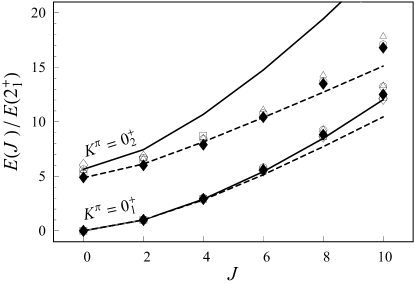
Figure 3: Yrast and $K^{\pi}=0^{+}_{2}$ band level energies, normalized to $E(2^{+}_{1})$, for ¹⁵⁰Nd (

$\square$

), ¹⁵²Sm ( $\circ$ ), ¹⁵⁴Gd (

$\vartriangle$

), ¹⁵⁶Dy (

$\blacksquare$

), and ¹⁶²Yb (

$\square$

). The predictions for X(5) (solid curve) and the sloped well with $S$$=$$50$ (dashed curve) are shown for comparison. Data are from Refs. nds1995:150 ; nds1996:152 ; nds1998:154 ; ndsboth:156 ; nds1999:162 ; mccutchan2004:162yb-beta .

The second order term in the $E2$ operator (7) can interfere either constructively or destructively with the first order term. For all transitions between low-lying levels considered here, the radial integrals $I_{1}$ and $I_{2}$ in (14) have the same sign. Thus, negative values of $A^{\prime}$ lead to constructive interference [note the negative coefficient in (14)], while positive values lead to destructive interference. For the X(5) square well, the higher-spin members of the yrast band have larger average $\beta$ values than do the low-spin members, so the quadratic term is relatively more important for the higher-spin levels. In the case of destructive interference, the curve showing the spin dependence of $B(E2)$ values, normalized to $B(E2;2^{+}_{1}\rightarrow 0^{+}_{1})$, falls below that obtained with the simple linear $E2$ operator, as seen in Fig. 4(a). The broad range of such curves obtained experimentally (see Ref. clark2003:x5-search ) can be qualitatively reproduced with different values of $A^{\prime}$. Destructive interference also reduces the interband $B(E2)$ strengths and the in-band $B(E2)$ strengths within the $K^{\pi}$$=$$0^{+}_{2}$ band, relative to $B(E2;2^{+}_{1}\rightarrow 0^{+}_{1})$ [Fig. 5(b)], ameliorating the overprediction of interband strengths in the X(5) model. The spin-descending interband transitions in the X(5) model have highly-suppressed linear $E2$ matrix elements, so these transitions are very sensitive to even a small quadratic contribution. Values of $A^{\prime}$ which give only moderate modifications to the other transitions can give complete destructive interference for these spin-descending transitions. The spin dependence of quadrupole moments within the yrast band is shown in Fig. 4(b).

Figure 4: Yrast band $B(E2)$ strengths and squared quadrupole moments, normalized to $B(E2;2^{+}_{1}\rightarrow 0^{+}_{1})$. (a,b) Values for the X(5) model ($S$$\rightarrow$$\infty$) calculated with a quadratic $E2$ transition operator, for $A^{\prime}$ ranging from $-1$ to $2$ in equal steps. (c,d) Values for the sloped well ($S$$=$50, 100, 200, 500, and $\infty$) calculated with a linear $E2$ transition operator.

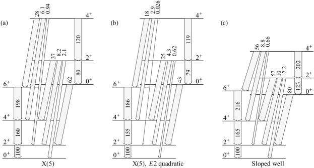
Figure 5: Level schemes and selected $B(E2)$ strengths for (a) the X(5) model with a linear $E2$ operator, (b) the X(5) model with a quadratic $E2$ operator ($A^{\prime}$$=$$0.7$), and (c) the sloped well ($S$$=$$50$) with a linear $E2$ operator. Arrow thicknesses are proportional to the logarithm of the $B(E2)$ strength.

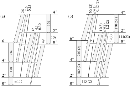
Figure 6: Level scheme and selected $B(E2)$ strengths (a) for the sloped well with parameters chosen to approximately reproduce the observed low-energy structure of ¹⁵⁰Nd ($S$$=$$75$, $A^{\prime}$$=$$0.6$) and (b) as measured for ¹⁵⁰Nd nds1995:150 ; kruecken2002:150nd-rdm . Arrow thicknesses are proportional to the logarithm of the $B(E2)$ strength. Limits are indicated on experimental $B(E2)$ strengths for transitions with unknown $E2/M1$ mixing ratios.

Observe that the situation just described differs considerably from that encountered for a pure rotor. For a rigid rotor, the intrinsic wave function $\Phi_{\alpha K}(\beta,\gamma)$ is the same for all levels within a band, so $I_{2}$ provides only a uniform adjustment to the intrinsic matrix element between bands. Inclusion of the second order term in $\mathfrak{M}(E2)$ thus leaves unchanged the ratio of any two $B(E2)$ values within a band or the ratio of any two $B(E2)$ values between the same two bands.

Although inclusion of a quadratic term in the $E2$ operator with $A^{\prime}$$>$$0$ can at least qualitatively explain the discrepancies between the X(5) $B(E2)$ predictions and empirical values, this explanation is not entirely satisfactory. Many different spin dependences of the $B(E2)$ values within the yrast band are observed for nuclei with similar energy spectra clark2003:x5-search , and these require correspondingly varied, apparently ad hoc choices of the parameter $A^{\prime}$ for their reproduction. Moreover, it is possible to obtain estimates for the coefficients $A_{1}$ and $A_{2}$ in the geometric $E2$ operator based on a simple model of the nuclear charge and current distribution, as described in Refs. hess1981:gcm-pt-os-w ; eisenberg1987:v1 , and these values yield $A^{\prime}$$\approx$$-0.2$, giving weak constructive interference for the low-lying transitions. In the interacting boson model, the $E2$ transition operator is of the form $T^{(E2)}$$\propto$$(d^{\dagger}\times\tilde{s}+s^{\dagger}\times\tilde{d})^{(2)}+\chi(d^{\dagger}\times\tilde{d})^{(2)}$, in terms of the boson creation operators $s^{\dagger}$ and $d^{\dagger}$, where the value $\chi$$=$$-\sqrt{7}/2$ is commonly used in calculations involving the transition from spherical to axially-symmetric deformed structure lipas1985:ecqf ; iachello1987:ibm . In the classical limit, $(d^{\dagger}\times\tilde{s}+s^{\dagger}\times\tilde{d})^{(2)}$ may be approximately identified with the linear term of the geometric model transition operator and $\chi(d^{\dagger}\times\tilde{d})^{(2)}$ with the quadratic term. The addition of these terms is constructive for low-lying transitions, and the relative contribution of the second-order term is comparable to that obtained for $A^{\prime}$$\approx$$-1$ in the present description.

The effect of sloped walls on the calculated $B(E2)$ strengths is dominated by the greater broadening of the well at high energies than at low energies discussed above. While all the eigenfunctions “spread” in $\beta$ extent relative to those for the square well, this spreading is most pronounced for the high-lying levels. Since the first order $E2$ operator is proportional to $\beta$, the $E2$ matrix elements tend to be enhanced for the higher-lying levels. In the yrast band, the in-band $B(E2)$ strengths for higher-spin band members are increased relative to those for the lower-spin band members, as are the quadrupole moments for higher-spin band members [Fig. 4(c,d)]. Several of the interband $B(E2)$ strengths are also increased relative to $B(E2;2^{+}_{1}\rightarrow 0^{+}_{1})$ (Fig. 5). The changes in $B(E2)$ values induced by decreasing $S$ are largely opposite in sense to those produced by introduction of the second-order term in the $E2$ operator. The parameters $S$ and $A^{\prime}$ may be chosen so as to balance these two effects against each other, except that for the spin-descending interband transitions the strong destructive interference tends to dominate.

To allow comparison with empirical values, in Fig. 6(a) predictions obtained with the sloped wall potential and quadratic $E2$ operator are shown for parameter values chosen to approximately reproduce the observed low-energy structure of ¹⁵⁰Nd. The experimental values are given in Fig. 6(b).

Finally, let us consider the effects of wall slope on the properties of the $K^{\pi}$$=$$2^{+}_{1}$ band, or $\gamma$ band. Within the $\gamma$-stabilized separation of variables of Ref. iachello2001:x5 , the properties of this band are largely independent of the specific choice of $\gamma$-confining potential $V_{\gamma}(\gamma)$. This potential determines the band head energy as well as the $\gamma$-dependent wave function $\eta(\gamma)$. The wave function, however, simply contributes a normalization factor $\int\left|\sin 3\gamma\right|d\gamma\eta_{1}(\gamma)\sin\gamma\eta_{0}(\gamma)$ to $I_{1}$ in (11), and an analogous factor to $I_{2}$, common to all electromagnetic matrix elements between the $K^{\pi}$$=$$2^{+}_{1}$ band and the $K^{\pi}$$=$$0^{+}_{1}$ and $0^{+}_{2}$ bands. Although these quantities can be calculated for any particular hypothesized form for $V_{\gamma}(\gamma)$, such as a harmonic oscillator potential iachello2001:x5 , they in practice may be treated as free parameters.

The essential feature of the $K^{\pi}$$=$$2^{+}_{1}$ band is that the radial wave function for each of its members is the “ground state” solution of the radial equation (3) for the given angular momentum. This $K^{\pi}$$=$$2^{+}_{1}$ band is thus essentially a duplicate of the yrast band, displaced to a higher energy by the excitation energy in the $\gamma$ degree of freedom, with energy spacings and radial wave functions for the even spin members identical to those for the yrast band, but with the addition of odd spin members and with different angular wave functions. (Note that for $K$$\neq$$0$ Bijker et al. bijker2003:x5-gamma use a different separation procedure from that in Refs. iachello2001:x5 ; bizzeti2002:104mo-x5 , yielding a modified form of the radial equation with $\alpha$$=$$\frac{1}{3}[L(L+1)-K^{2}]+2$, which changes the energy spacings and in-band radial matrix elements by $\lesssim$$5\%$ relative to those of the yrast band.) Thus, the dependence of $K^{\pi}$$=$$2^{+}_{1}$ band properties upon wall slope closely matches that of the yrast band properties. Notably, the $K^{\pi}$$=$$2^{+}_{1}$ band does not demonstrate the rapid decrease in energy spacing scale with decreasing wall slope exhibited by the $K^{\pi}$$=$$0^{+}_{2}$ band, as illustrated in Fig. 7(a). This is at least qualitatively consistent with the observed similarity of the yrast and $K^{\pi}$$=$$2^{+}_{1}$, but not $K^{\pi}$$=$$0^{+}_{2}$, band energy spacings in the $N$$=$90 X(5) candidate nuclei.

Figure 7: Dependence of properties of the $K^{\pi}$$=$$2^{+}_{1}$ band upon wall slope. Values are shown for the X(5) model (solid line), $S$$=$100 (long-dashed line), $S$$=$50 (short-dashed line), and $S$$=$25 (dotted line). (a) Yrast, $K^{\pi}$$=$$0^{+}_{2}$, and $K^{\pi}$$=$$2^{+}_{1}$ band energies, illustrating the identical dependences of the yrast and $K^{\pi}$$=$$2^{+}_{1}$ bands. The $K^{\pi}$$=$$2^{+}_{1}$ band head energy is arbitrary (see text). (b) $B(E2)$ branching ratios for $\Delta J$$=$$\pm 2$ transitions from the $K^{\pi}$$=$$2^{+}_{1}$ band to the yrast band. (c,d) $B(E2)$ strengths for $\Delta J$$=$$\pm 2$ transitions from the $K^{\pi}$$=$$2^{+}_{1}$ band to the $K^{\pi}$$=$$0^{+}_{2}$ band, normalized to $B(E2;2^{+}_{\gamma}\rightarrow 0^{+}_{1})$. The separation of variables of Refs. iachello2001:x5 ; bizzeti2002:104mo-x5 has been used for all calculations.

Since the even spin members of the $K^{\pi}$$=$$2^{+}_{1}$ band possess the same radial wave functions as the yrast band members, the strengths of transitions within the $K^{\pi}$$=$$2^{+}_{1}$ band or between this band and the yrast band depend upon the same radial matrix elements as do the yrast in-band transition strengths and quadrupole moments already considered. Consequently, decreasing wall slope leads to a moderate enhancement of the interband transition strengths involving higher spin levels, directly commensurate with the increases shown in Fig. 4(c,d). The dependence of branching ratios from the $K^{\pi}$$=$$2^{+}_{1}$ band to the yrast band on wall slope is shown in Fig. 7(b). Transitions between the $K^{\pi}$$=$$2^{+}_{1}$ band and the $K^{\pi}$$=$$0^{+}_{2}$ band depend instead upon radial matrix elements which contribute to the $K^{\pi}$$=$$0^{+}_{2}$ to yrast band transition strengths. (The small radial matrix element values which yield the characteristic suppression of spin-descending transitions from the $K^{\pi}$$=$$0^{+}_{2}$ band to the yrast band here yield a suppression of spin-ascending $K^{\pi}$$=$$2^{+}_{1}$ to $0^{+}_{2}$ transitions.) Decreasing wall slope yields enhancement of the allowed transitions and, for the low-spin levels, either little change or substantial reduction of the suppressed transitions [Fig. 7(c,d)]. Detailed quantitative predictions for the $K^{\pi}$$=$$2^{+}_{1}$ band level energies and electromagnetic observables, using either the separation of variables of Refs. iachello2001:x5 ; bizzeti2002:104mo-x5 or that of Ref. bijker2003:x5-gamma , may be obtained with the provided code swell-epaps .

IV Conclusion

The use of a $\beta$-soft potential within the geometric picture has recently received attention as providing a simple description of nuclei intermediate between spherical and rigidly deformed structure. From the present results, it is seen that the energy spacing scale of states within excited bands is highly sensitive to the stiffness of the well boundary wall. A potential for which the well width increases with energy can produce a more compact spacing scale for excited states than is obtained with a pure square well, providing much closer agreement with the observed energy spectra for nuclei in the $N$$\approx$$90$ transition region. It is also found that a second-order contribution to the $E2$ transition operator can lead to a wide range of possible yrast band $B(E2)$ spin dependences, as well as to modifications of off-yrast matrix elements. However, a systematic understanding of the proper strength for this second-order contribution is needed if the $E2$ operator is to be applied effectively.

- (1) F. Iachello, Phys. Rev. Lett. 85, 3580 (2000).
- (2) F. Iachello, Phys. Rev. Lett. 87, 052502 (2001).
- (3) L. Wilets and M. Jean, Phys. Rev. 102, 788 (1956).
- (4) A. Bohr and B. R. Mottelson, Nuclear Deformations, Vol. 2 of Nuclear Structure (World Scientific, Singapore, 1998).
- (5) R. F. Casten and N. V. Zamfir, Phys. Rev. Lett. 87, 052503 (2001).
- (6) P. G. Bizzeti and A. M. Bizzeti-Sona, Phys. Rev. C 66, 031301(R) (2002).
- (7) R. Krücken, B. Albanna, C. Bialik, R. F. Casten, J. R. Cooper, A. Dewald, N. V. Zamfir, C. J. Barton, C. W. Beausang, M. A. Caprio, A. A. Hecht, T. Klug, J. R. Novak, N. Pietralla, and P. von Brentano, Phys. Rev. Lett. 88, 232501 (2002).
- (8) D. S. Brenner, in Mapping the Triangle, edited by A. Aprahamian, J. A. Cizewski, S. Pittel, and N. V. Zamfir, AIP Conf. Proc. 638 (AIP, Melville, NY, 2002), p. 223.
- (9) M. A. Caprio, N. V. Zamfir, R. F. Casten, C. J. Barton, C. W. Beausang, J. R. Cooper, A. A. Hecht, R. Krücken, H. Newman, J. R. Novak, N. Pietralla, A. Wolf, and K. E. Zyromski, Phys. Rev. C 66, 054310 (2002).
- (10) C. Hutter, R. Krücken, A. Aprahamian, C. J. Barton, C. W. Beausang, M. A. Caprio, R. F. Casten, W.-T. Chou, R. M. Clark, D. Cline, J. R. Cooper, M. Cromaz, A. A. Hecht, A. O. Macchiavelli, N. Pietralla, M. Shawcross, M. A. Stoyer, C. Y. Wu, and N. V. Zamfir, Phys. Rev. C 67, 054315 (2003).
- (11) R. M. Clark, M. Cromaz, M. A. Deleplanque, M. Descovich, R. M. Diamond, P. Fallon, R. B. Firestone, I. Y. Lee, A. O. Macchiavelli, H. Mahmud, E. Rodriguez-Vieitez, F. S. Stephens, and D. Ward, Phys. Rev. C 68, 037301 (2003).
- (12) E. A. McCutchan, N. V. Zamfir, M. A. Caprio, R. F. Casten, H. Amro, C. W. Beausang, D. S. Brenner, A. A. Hecht, C. Hutter, S. D. Langdown, D. A. Meyer, P. H. Regan, J. J. Ressler, and A. D. Yamamoto, Phys. Rev. C 69, 024308 (2004).
- (13) R. Bijker, R. F. Casten, N. V. Zamfir, and E. A. McCutchan, Phys. Rev. C 68, 064304 (2003).
- (14) E. der Mateosian and J. K. Tuli, Nucl. Data Sheets 75, 827 (1995).
- (15) A. Artna-Cohen, Nucl. Data Sheets 79, 1 (1996).
- (16) C. W. Reich and R. G. Helmer, Nucl. Data Sheets 85, 171 (1998).
- (17) R. G. Helmer, Nucl. Data Sheets 49, 383 (1986); 65, 65 (1992).
- (18) O. Scholten, F. Iachello, and A. Arima, Ann. Phys. (N.Y.) 115, 325 (1978).
- (19) Jing-Ye Zhang, M. A. Caprio, N. V. Zamfir, and R. F. Casten, Phys. Rev. C 60, 061304(R) (1999).
- (20) R. M. Clark, M. Cromaz, M. A. Deleplanque, R. M. Diamond, P. Fallon, A. Görgen, I. Y. Lee, A. O. Macchiavelli, F. S. Stephens, and D. Ward, Phys. Rev. C 67, 041302 (2003).
- (21) R. F. Casten, N. V. Zamfir, and R. Krücken, Phys. Rev. C 68, 059801 (2003).
- (22) J. M. Arias, Phys. Rev. C 63, 034308 (2001).
- (23) N. Pietralla and O. M. Gorbachenko (in preparation).
- (24) See EPAPS Document No. E-PRVCAN-69-019404 for computer code for solution of the sloped well eigenproblem and calculation of matrix elements. The code also calculates observables for the E(5) and X(5) models. This document may be retrieved via the EPAPS home page (http://www.aip.org/pubservs/epaps.html) or by FTP (ftp://ftp.aip.org/epaps/).
- (25) G. Rakavy, Nucl. Phys. 4, 289 (1957).
- (26) D. R. Bès, Nucl. Phys. 10, 373 (1959).
- (27) G. Gneuss and W. Greiner, Nucl. Phys. A 171, 449 (1971).
- (28) P. O. Hess, J. Maruhn, and W. Greiner, J. Phys. G 7, 737 (1981).
- (29) J. M. Eisenberg and W. Greiner, Nuclear Models: Collective and Single-Particle Phenomena, Vol. 1 of Nuclear Theory (North-Holland, Amsterdam, 1987), 3rd ed.
- (30) The operator as defined in (6) is consistent with the leading-order operator of Bohr and Mottelson bohr1998:v2 , but the complex conjugate definition is also encountered eisenberg1987:v1 .
- (31) The function used here is that of Rose rose1957:am , which is the complex conjugate of the function defined by Bohr and Mottelson bohr1998:v2 .
- (32) M. E. Rose, Elementary Theory of Angular Momentum (John Wiley & Sons, New York, 1957).
- (33) M. A. Caprio, Phys. Rev. C 68, 054303 (2003).
- (34) R. G. Helmer and C. W. Reich, Nucl. Data Sheets 87, 317 (1999).
- (35) P. O. Lipas, P. Toivonen, and D. D. Warner, Phys. Lett. B 155, 295 (1985).
- (36) F. Iachello and A. Arima, The Interacting Boson Model (Cambridge University Press, Cambridge, 1987).