Effect of hard processes on momentum correlations

Abstract

The effect of hard processes to be encountered in HBT studies at the Large Hadron Collider have been studied. A simple simulation has allowed us to generate momentum correlations involving jet particles as well as particles originating from the kinetic freeze out and to compare them to a simple theoretical model which has been developed. The first results on the effect of hard processes on the correlation function for the case of jet quenching are presented.

1 Introduction

Momentum correlations of pions and kaons created in heavy ion collisions have been extensively studied in a wide energy range from the AGS through SPS and finally at RHIC [1]. The purpose of these studies is to get information on the dimensions of the phase space from which the particles have been emitted [2]. However, interpretation of the data measured at RHIC has been proven to be problematic and is not yet completely understood (see e.g. [3]).

Looking ahead towards LHC one can wonder what are momentum correlations going to look like in presence of an important contribution of hard processes. If we assume that the source is a superposition of jet sources and a thermal fireball then the resulting correlations should reflect contributions from:

• pairs of particles from a single jet, which will reflect dimension of the region where the jet fragmented;

• pairs of particles from different jets, which will be given by the size of the initial collision volume;

• pairs where both particles stemming from the decoupling of thermal fireball (larger than the initial collision volume);

• pairs where one particle comes from the thermal fireball and the other one is produced from jet fragmentation.

In this paper we describe a toy model to simulate the effects listed above. We provide analytical calculations of the correlation function in a special limiting case. Then we investigate how particle production from jet fragmentation shows itself in the correlation data. We study the visibility of the effect at different proportions of jet production to the total multiplicity and at different transverse momenta.

2 Simulation

Jets.

With Pythia [4] we simulate p+p collisions at $\sqrt{s}=5.5\,\mbox{TeV}$. We extract jets in pseudorapidity coverage of the ALICE detector $-1<\eta<1$, by making use of a simple clustering algorithm. We identify the highest $p_{t}$ particle among fragmentation products of a single string as the leading one and then search for particles with an opening angle $\Delta\phi$ and relative rapidity $\Delta\eta$ to the leading one that fulfills criterion: $\sqrt{{\Delta\phi}^{2}+{\Delta\eta}^{2}}<2$. Jets with the sum of $p_{t}$’s from all particles between 5 and 10 GeV are selected for further study.

Within the jet, the original position of the particles is distributed according to a Gaussian of the width $J$ and all particles are assumed to be produced instantaneously

$$s(x;x_{j})=\frac{1}{(2\pi\,J^{2})^{3/2}}\,\exp\left(-\frac{(\vec{x}-\vec{x}_{j})^{2}}{2\,J^{2}}\right)\,\delta(t-t_{j})\,.$$ (1)

The jet itself is placed into a random position $(\vec{x}_{j},\,t_{j})$.

Jet quenching model.

We model the strong jet suppression by a very dense medium by assuming that the jets originate from surface of a cylinder with radius $R$ and length $L$. Eventually, we allow for some finite thickness $\delta R$ for the cylinder surface. It is assumed that the total transverse momentum of the jet is always perpendicular to the cylinder surface and that jets are produced instantaneously.

Non-quenching model.

If the early medium does not suppress jets, we should be able to observe jets from hard collisions in all reaction volume. We model such a case by choosing a Gaussian distribution of the jets in the transverse plane, but we keep the uniform distribution in longitudinal direction from $-L/2$ to $L/2$. Instantaneous production is assumed.

Background.

Apart from jet fragmentation, particles can be produced by thermal fireball. If we are interested in jets, these particles represent background for us. Its momentum distribution is such that the total resulting spectrum at low $p_{t}$ is given by

$$F(p_{t})=\frac{d^{2}N}{p_{t}\,dp_{t}\,dy}\propto\exp\left(-\frac{m_{t}}{T}\right)\,,$$ (2a)

where $T$ is an effective slope parameter. The background spectrum is defined as $F_{b}(p_{t})=F(p_{t})-F_{j}(p_{t})$, where $F_{j}(p_{t})$ the spectrum produced by jets.

At high $p_{t}$ the spectrum is dominantly shaped by jet fragmentation. Technically, it eventually shows up when $F_{j}(p_{t})$ supersedes parametrisation (2a). In order to obtain a smooth total spectrum with exponential low-$p_{t}$ part and high-$p_{t}$ tail as given by jets, we choose the normalization of the background spectrum $F_{b}(p_{t})=F(p_{t})/2$ when the jet contribution becomes $F_{j}(p_{t})>F(p_{t})/2$.

The background particles are assumed to be produced instantaneously at the same time as the jets and are distributed in space according to a Gaussian

$$S_{b}(x,p)=F_{b}(p)\frac{1}{(2\pi B^{2}(p_{t}))^{3/2}}\,\exp\left(-\frac{\vec{x}^{2}}{2B^{2}(p_{t})}\right)\,\delta(t-t_{0})\,.$$ (2b)

The size of the background source first decreases linearly with $p_{t}$ up to $p_{t}={p_{t}^{\rm max}}$ and than stays constant:

$$B=\begin{cases}B_{0}\frac{p_{t}^{\rm max}-p_{t}}{p_{t}^{\rm max}}+B_{\rm max}\frac{p_{t}}{p_{t}^{\rm max}}&\mbox{for}\quad p_{t}<p_{t}^{\rm max}\\ B_{\rm max}&\mbox{for}\quad p_{t}\geq p_{t}^{\rm max}\end{cases}\,,$$ (2c)

where we can specify $B_{0}$, $B_{\rm max}$, and $p_{t}^{\rm max}$.

Correlation function.

These are constructed in the so-called out-side-long coordinate frame by making use of the weighting algorithm due to Lednický [5] within the ALICE HBT analysis package HBTAN [6].

3 Theoretical understanding

If we specify the emission function of the source $S(x,p)$, correlation function can be calculated from

$$C(q,K)-1=\frac{\left|\int d^{4}x\,\exp(i\,q\cdot x)\,S(x,K)\right|^{2}}{\left(\int d^{4}x\,S(x,K)\right)^{2}}\,.$$ (3)

If there are two or more jets in an event, and we sum over a large number of events, we can express the emission function by integrating over all possible locations of the “jet centres”

$$S(x,p)\propto\int dx_{j}\,D(x_{j},p)\,s(x;x_{j})\,,$$ (4)

where $s(x;x_{j})$ was specified in eq. (1) and $D(x_{j},p)$ is the distribution of jet centres, which lead to production of momentum $p$. There may be additional dependence of $S(x,p)$ on the momentum, but this is irrelevant for calculating the correlation function.

For the case of jets produced at cylinder surface we write

$$D(x_{j},p)=D(t_{j},r_{j},\varphi_{j},z_{j})=\\ \exp\left(\frac{\cos\varphi_{j}}{\Phi}\right)\,\delta(r_{j}-R)\,\Theta(z_{j}-L/2)\,\Theta(L/2-z_{j})\,\delta(t_{j}-t_{0})\,.$$ (5)

For simplicity, we neglect the possibility of finite thickness of the surface here. The factor $\exp(\cos\varphi_{j}/\Phi)$ allows particles to be produced under some angle with respect to the jet angle. Since we assume that the jet momentum is perpendicular to the surface, and we work in the out-side-long system, $\varphi_{j}$ is the angle between $\vec{p}_{t}$ of the particle and the radial jet coordinate $\vec{r}$. Parameter $\Phi$ regulates the broadness of the jet: $\Phi\ll 1$ leads to very focussed jets, while $\Phi\to\infty$ leaves us with uncollimated particle production. In principle, $\Phi$ depends on particle momentum, but we will suppress this dependence here for simplicity.

Correlation function can be calculated from eq. (3):

$$C(q_{o},q_{s},q_{l})-1=\exp\left(-(q_{o}^{2}+q_{s}^{2}+q_{l}^{2})J^{2}\right)\,\frac{4}{q_{l}^{2}\,L^{2}}\,\sin^{2}\left(\frac{q_{l}\,L}{2}\right)\frac{1}{(2\pi)^{2}\,\mbox{I}_{0}^{2}(1/\Phi)}\,\\ \times\left|\int_{-\pi}^{\pi}d\varphi\,\exp\left[i\,R\,(q_{o}\,\cos\varphi+q_{s}\,\sin\varphi)\right]\,\exp\left(\frac{\cos\varphi}{\Phi}\right)\right|^{2}\,,$$ (6)

where $\mbox{I}_{0}$ is the modified Bessel function. For qualitative understanding it is useful to examine the limit $\Phi\to\infty$ when one can analytically calculate the cuts of the correlation function along the $q$-axes

$$C(q_{o},q_{s}=0,q_{l}=0)-1 = \exp(-J^{2}\,q_{o}^{2})\,\left\{\mbox{J}_{0}^{2}(q_{o}\,R)+\mbox{H}_{0}^{2}(|q_{o}\,R|)\right\}\,,$$ (7a)

$$C(q_{o}=0,q_{s},q_{l}=0)-1 = \exp(-J^{2}\,q_{s}^{2})\,\mbox{J}_{0}^{2}(q_{s}\,R)\,,$$ (7b)

$$C(q_{o}=0,q_{s}=0,q_{l})-1 = \exp(-J^{2}\,q_{l}^{2})\,\frac{4}{q_{l}^{2}\,L^{2}}\,\sin^{2}\left(\frac{q_{l}\,L}{2}\right)\,,$$ (7c)

where $\mbox{J}_{0}$ is a Bessel function and $\mbox{H}_{0}$ is a Struve function.

If a background source is added, the correlation function includes contributions of pairs of jet particles, background particles and those with one particle from a jet and one from background. The analytical expression thus becomes more complicated.

Finally, we also made simulations with jets produced from a Gaussian distribution. Calculations similar to those in this section show that such a distribution of jets leads to a Gaussian correlation function.

4 Results

Only jets.

First, we analyze events that contain jets only (and no background). We assume cylindrical geometry with radius of $R=6\,\mbox{fm}$, $\delta R=1\,\mbox{fm}$, and length $L=1\,\mbox{fm}$ (Fig. 1) or $L=2\,\mbox{fm}$ (Fig. 2). Jet radius $J$ is 1 fm.

Figure 1: Correlation function resulting from simulation of 10 jets produced at the surface of a cylinder with the radius 6 fm and length 1 fm. Plotted are cuts along $q$-axes.

Figure 2: Correlation function resulting from simulation of 100 jets from a surface of a cylinder with the radius 6 fm and length 2 fm. Curves correspond to a fit with the theoretical curve given by eq. (6) multiplied by interception parameter $\lambda=0.77$. Parameters of the curves are: $R=5.92\,\mbox{fm}$, $J=1.06\,\mbox{fm}$, $L=1.82\,\mbox{fm}$, and $\Phi=0.86$.

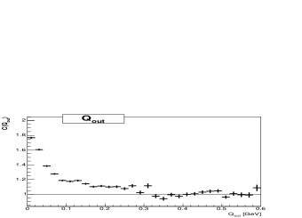
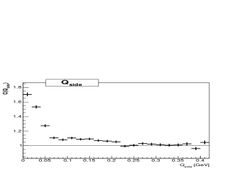
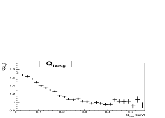
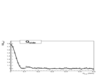
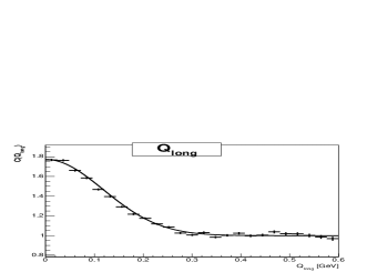
In Figures 1 and 2 we show the projections of the correlation functions from simulations with 10 and 100 jets, respectively. In the latter case the simulated correlation function is rather well reproduced by theoretical curves which were calculated from eq. (6). A parameter $\lambda<1$ which multiplies the theoretical expression was added in order to account for the intercept of $C(q=0)$ which is smaller than 2 because in obtaining the projections we always integrated over finite regions in the remaining two $q$-coordinates.

The structure of the projection in $q_{s}$ in Fig. 2 can be understood from the $\Phi\to\infty$ limit formula, eq. (7b): the sub-leading peaks stem from the Bessel function. A similar structure in $q_{o}$ is “dissolved” faster when the jet collimation is finite and leads to the “shoulder” in Fig. 2 (left). Projection in $q_{l}$ can be reproduced by eq. (7c).

In the simulation, the angular width of the jet depends on transverse momentum of particles. Thus $\Phi$ is not constant. It appears that averaging over $\Phi(p_{t})$ is more important in case of a smaller number of jets. Projections in $q_{o}$ and $q_{s}$ in Fig. 1 result from such averaging and we cannot describe them with the prescription (6). Beyond the leading peak we do not see any clear subleading maxima, but the correlation function assumes a shoulder-like shape at larger $q$’s.

Jets with background.

If in addition to jets there is also other source of particles, the characteristic features of the correlation function due to jets get diluted. We study this by adding a background source, as described by eqs. (2). We choose $T=210\,\mbox{MeV}$, $B_{0}=10\,\mbox{fm}$, $B_{\rm max}=1\,\mbox{fm}$, and $p_{t}^{\rm max}=1.2\,\mbox{GeV}$.

Figure 3: Correlation function resulting from simulation of 100 jets from a surface of a cylinder with the radius 6 fm and a “thermal” background source; 2/3 af all pions come from jets. Plotted are cuts along $q$-axes.

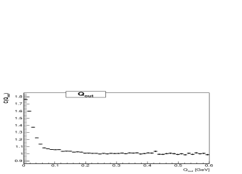
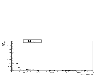
In Figure 3 we plot the correlation function resulting from a simulation with 100 jets where only 1/3 of the pions are produced by the background. The dimensions of the background source (averaged over $p_{t}$) are comparable with the transverse size of the source of jets, while they are clearly larger than it in the longitudinal direction. Therefore, for the two transverse $q$-components the background just weakens the characteristic shape from jets. On the other hand, in $q_{l}$ a narrow peak at $q_{l}=0$ results from the large size of the background.

We checked that if the percentage of jet pions drops as low as 1/6, the $p_{t}$-integrated correlation function is completely determined by the background source and no signal of jets is seen. Note that the proportion of jet particles can be even lower at ALICE: at midrapidity we assume 3000 for $dN/dy$ of charged particles, out of which about 90% are pions, so we obtain roughly 1350 single-charge pions. Since a jet produces on average 2.4 positive pions in our acceptance region, 100 observable jets with pseudorapidity $-1<\eta<1$ will leave us with 120 single-charge pions per pseudorapidity unit. That makes the ratio of pions from jets to the total pion number about $120/1350\sim 1/11$. (We explore this situation in the next paragraph.)

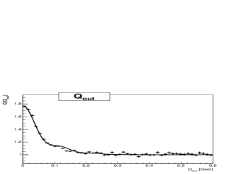
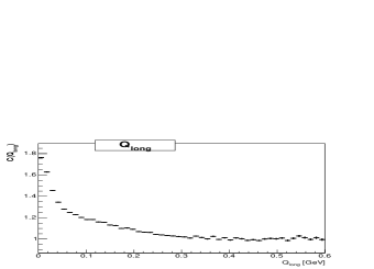
High $p_{t}$.

Figure 4: Correlation function resulting from simulation of 100 jets from a surface of a cylinder with the radius 6 fm and a “thermal” background source; 1/12 of all particles come from jets and a cut is imposed: $K_{t}>1.2\,\mbox{GeV}/c$. Plotted are cuts along $q$-axes together with Gaussian fits.

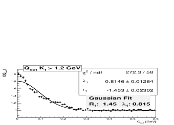
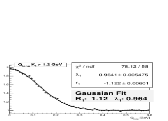
In order to eliminate the effect of the background we can focus on particles with high transverse momenta where we expect the portion of jet-produced pions to be increased. In Figure 4 we plot correlation function calculated for jets with a background source as previously, but we use only particle pairs with $K_{t}$ above 1.2 GeV in our analysis. A non-Gaussian shape, particularly in $q_{o}$ and slightly in $q_{s}$, is observed, which is due to contribution from jets.

We have also simulated jet production from a source with Gaussian transverse profile together with background and imposed the same contraint on $K_{t}$ (not shown). This leads to similar non-Gaussian shapes of the correlation function as shown in Fig. 4. A more detailed study of the shape of the correlation function is neccessary in order to understand differences between the two models for jet distribution.

5 Conclusions

• Correlation functions are affected if there are pions produced from fragmentation of jets.

• Correlation functions assume particularly characteristic shape if there is strong suppression of jets due to energy loss of the leading parton in a deconfined medium.

In the latter case, jets are effectively emitted only from the surface of the fireball. Presumably, these characteristic shapes are dissolved in real data because there are much more particles stemming from thermal fireball.

Correlation signal of individual jets is not visible if the total number of particles in the bin is much larger than the number of particles produced by a jet. We can estimate the contribution to each bin of correlation function as $N_{tot}^{2}$ ($N_{tot}$ is total number of particles). We write $N_{tot}=N_{j}+N_{b}$, where $N_{j}$ is the number of particles produced by jets and $N_{b}$ the number of particles coming from the thermal source. Then the number of pairs is written as $(N_{j}+N_{b})^{2}={N_{j}}^{2}+2N_{j}N_{b}+{N_{b}}^{2}$. In our study, ${N_{j}}^{2}$ corresponds to signal, ${N_{b}}^{2}$ to background, and $N_{j}N_{b}$ is the correlation between particles of signal and background. If $N_{j}\ll N_{b}$, the signal becomes invisible.

• The influence of background can be limited by using only pairs with high transverse pair momentum $K_{t}$ in the analysis.

Although we couldn’t describe the correlation function obtained after such a cut-off by our analytical expressions, we could observe a clear deviation from Gaussian shape. Note that Gaussian shape would result from our background source in the absence of jets. A non-Gaussian shape can influence results of fitting real data by Gaussian parametrisation and may cause problems when interpreting such a fit. We have shown that jets lead to structures in the correlation functions at large momentum differences: beyond the main peak at $q=0$. Thus it is also important to look at the large-q region in order to learn about the characteristics of the source.

References

- [1] B.Tomášik and U.A.Wiedemann, in: Quark Gluon Plasma 3, R.C. Hwa and X.-N. Wang eds., World Scientific, 2004, [hep-ph/0210250].
- [2] U.W. Heinz and U.A. Wiedemann, Phys. Rep. 319 (1999) 145.
- [3] U.W. Heinz and P.F. Kolb, hep-ph/0204061.
- [4] T. Sjöstrand et al., Computer Phys. Commun. 135 (2001) 238.
- [5] R. Lednický and V.L. Lyuboshitz, Sov. J. Nucl. Phys. 35, 770 (1982); Proc. CORINNE 90, Nantes, France, 1990 (ed. D. Ardouin, World Scientific, 1990) p. 42.
- [6] P.K. Skowroński for ALICE Collaboration, physics/0306111.