Regge Behavior of DIS Structure Functions

Abstract

Building on previous works of the mid 1960’s, we construct an integral equation for forward elastic scattering ($t=0$) at arbitrary virtuality $Q^{2}$ and large $s=W^{2}$. This equation sums the ladder production of massless intermediate bosons to all orders, and the solution exhibits Regge behavior. The equation is used to study scattering in a simple $\chi^{\dagger}\chi\phi$ scalar theory, where it is solved appoximately and applied to the study of DIS at small $x$. We find that the model can naturally describe the quark distribution in both the large $x$ region and the small $x$ region dominated by Reggeon exchange.

0

I Introduction

This paper discusses the ingredients of a theory of deep inelastic scattering (DIS) that holds for all values of the Bjorken scaling variable $x=Q^{2}/2M_{B}\nu$ (where $M_{B}$ is the mass of the target bound state). The $Q^{2}$ of the virtual photon is fixed at a large value, so the $Q^{2}$ evolution of the structure functions will not be discussed. The individual ingredients are well known; our emphasis here is on combining these into a unified picture and in explaining how the various pieces fit together.

At large $Q^{2}$, the QCD coupling $\alpha_{s}$ is small, and the strong interaction dynamics can be treated perturbatively (i.e. to lowest order) except in regions where contribution from higher order loops are enhanced, so that contributions of all orders must be summed. It is well known that the existence of the bound state itself (the target $q\bar{Q}$ system in the simple example discussed in this paper) depends on the enhancement of ladder type loops, so the description of the bound state vertex function must involve nonperturbative physics. Nonperturbative contributions are also known to be important in the region of small $x$ Feynman ; Ioffe ; Yn ; Kaidalov . In the 1960’s it was shown that Regge behavior is generated by infinite sums of ladder diagrams in the $t$-channel and explicit equations have been written down for these ladder-type amplitudes Bertocci ; Simonov and solved analytically and numerically [6]. Furthermore, it was shown in the case of DIS that the finite scaling limit in $x$ of structure functions with Regge behaviour is possible to obtain if the Regge residues are properly tuned [7]. In what follows we derive explicitly the Regge behaviour of structure functions in our model and show that it agrees with general expectations [1-4] and the conjecture made in Ref. Abarb .

These basic ideas, and the specific model discussed in this paper, are illustrated in Fig. 1. The two diagrams show contributions to DIS from a bound state of a heavy anti-quark (or diquark, if applied to baryons) $\bar{Q}$ of mass $M$ (assumed to have no charge, for simplicity) and a light quark $q$ of mass $m$, interacting through the exchange of scalar gluons ($\phi$ particles with mass $\mu$; confinement is neglected in this discussion). To simulate some aspects of the behavior of QCD at high $Q^{2}$, the “quark-gluon” coupling, $g$, will be assumed to be small. Even for small couplings bound states exist (as in atomic physics, for example); they emerge from the infinite sum of ladder-like diagrams in the bound state $s$-channel grosstext . The second diagram, Fig. 1(b), describes contributions from the expansion of higher $q\bar{Q}\phi^{n}$ Fock states, and would normally be suppressed by the smallness of the coupling constant $g$. These diagrams are indeed small, except in the region of large $Q^{2}$ and small $x$, where each of the loops in the $t$-channel ladder sum is large, and contributions of this type must be summed to all orders. This nonperturbative contribution was discussed in Ref. Simonov , and shown to exhibt Regge-like behavior.

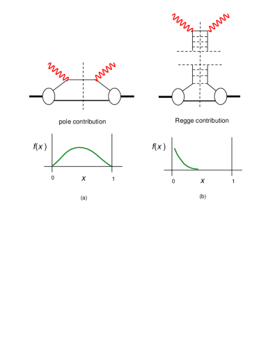
Figure 1: The two contributions to DIS studied in this paper. (a) Pole contribution, important at medium to large $x$. (b) Regge contribution arising from the contributions of higher Fock components, which dominates at small $x$. The expected qualitative behavior of each contribution is shown below each diagram.

In accordance with Regge theory [1-4,7], at small $x$ the quark distributions $F_{1}$ and $F_{2}$ should scale as

$$W_{1}(Q^{2},x)\to F_{1}(x) \simeq \lambda_{1}\left(\frac{1}{x}\right)^{\ell(0)}$$ (1)

$$\nu W_{2}(Q^{2},x)\to F_{2}(x) \simeq \lambda_{2}\left(\frac{1}{x}\right)^{\ell(0)-1}$$ (2)

where $\ell(0)$ is the intercept of the corresponding Regge trajectory. The valence quark distributions $f(x)=F_{2}(x)/x$ are known to behave at small $x$ as $x^{-0.5}$ while for sea quarks this behavior is $x^{-1}$, corresponding to the Regge trajectories of the $\rho$ meson and pomeron respectively Kaidalov . However the direct matching of the Regge pole contribution to the scaling behavior at larger $x$ requires a specific tuning of the coefficients $\lambda_{i}$, which is not known on general grounds [2]. The relevant behaviour of these coefficients was suggested in Ref. Abarb based on the available solutions of scalar ladder equations with a special relation between the masses Nakan or upper bounds for the massive case Trei . It would be instructive to use one solvable model with Regge behavior to understand how the small $x$ behavior explicitly matches with the behavior at $x$ around one.

This is the primary purpose of the present paper: to show how these two processes can be added together to produce a description of DIS valid for all $x$. We will carry out this discussion using the covariant spectator equation in the ladder approximation gross .

Our treatment of the diagram 1(b) is based on the integral equation for the imaginary part of the amplitude for the scattering of two scalar particles of mass $m$ in the scalar $\chi^{2}\phi$ theory, derived independently by similar, but slightly different methods, in Refs. Bertocci and Simonov . From this equation, which essentially sums up ladder-type diagrams, the intercept of a Regge trajectory was found analytically. It appears that this integral equation is a very useful tool for studying structure functions, as will be seen in what follows.

This paper is divided into five sections. In the next section we derive the integral equation for forward $\gamma q$ elastic scattering, allowing the external photons to have large $Q^{2}$, which is relevant to applications to DIS, and the quark to have a virtual mass $p^{2}\neq m^{2}$, needed for the application to bound quarks. In Sec. III we solve the equation, and in Sec. IV we add the photon spin (which was neglected in Sec. III for simplicity), and explicily evaluate the two diagrams shown in Fig. 1. Our conclusions are presented in Sec. V and the Appendices include some further details.

This work can be easily extended to the description of non-forward scattering, and can be used to model Generalized Parton Distributions (GPD’s) Radyushkin ; Ji ; Diehl:2003ny which is one of the motivations of the present work, but these applications are saved for later papers.

II Integral equation for photon-quark scattering

The integral equation to be derived is illustrated in Fig. 2. We have specialized the kinematics to forward scattering, appropriate to applications to DIS, and assume here that the photon has zero spin (this will be corrected in Sec. IV). (A more general equation applicable at momentum transfers $t\neq 0$ can be derived using the methods of Refs. Bertocci ; Simonov , and will be discussed elsewhere.)

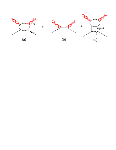
Figure 2: Diagrammatic representation of Eq. (23). The solid lines are “quarks” of mass $m$, the horizontal dashed line is a “gluon” of mass $\mu\to 0$, and the vertical dashed line reminds us that all intermediate particles are on shell. Fig.(b) is the pole term.

The integral equation can be easily obtained from study of the box diagram, Fig. 3. The imaginary part of this amplitude is the total forward cross section for the process $\gamma+q\to q+g$. Hence

$${\rm Im}T_{2} = e^{2}g^{2}\int\frac{d^{3}kd^{3}p}{(2\pi)^{6}4\omega_{k}E_{p^{\prime}}}\frac{(2\pi)^{4}\delta^{4}(k+p^{\prime}-q-p)}{[m^{2}-(p-k)^{2}]^{2}}$$ (3)

$$= \frac{e^{2}g^{2}}{16\pi^{2}}\int\frac{d^{3}k\,\delta(E_{p^{\prime}}+\omega_{k}-p_{0}-q_{0})}{\omega_{k}E_{p^{\prime}}\,[m^{2}-(p-k)^{2}]^{2}}\,,$$

where $e$ is the charge of the quark, and $\omega_{k}=\sqrt{\mu^{2}+k^{2}}$ and $E_{p^{\prime}}=\sqrt{m^{2}+p^{\prime 2}}$. Since $q^{2}=-Q^{2}<0$, it is convenient to evaluate this integral in the Breit frame, where

$$q = (0,0,0,Q)$$

$$p = (p_{0},0,0,p_{z})\,.$$ (4)

[The external quark is off-shell, and its energy is fixed by other variables.] Then the integrand is independent of the azymuthal angle, and the delta function may be used to evaluate the integral over $k_{\perp}^{2}$, giving

$${\rm Im}T_{2}(s,x,Q^{2}) = \frac{e^{2}g^{2}}{8\pi}\int_{k^{-}_{z}}^{k^{+}_{z}}\frac{dk_{z}}{p_{0}}\frac{1}{[m^{2}-(p-k)^{2}]^{2}}\,,\quad$$ (5)

where we have introduced the variables

$$s = (p+q)^{2}=p^{2}+Q^{2}\left(\frac{1}{x}-1\right)\geq(m+\mu)^{2}$$

$$x = \frac{Q^{2}}{2p\cdot q}=-\frac{Q}{2p_{z}}\,.$$ (6)

Note that, because the external quark is off-shell, $x$ is not restricted, and

$$p_{0}^{2}=s+Q^{2}\left(1-\frac{1}{2x}\right)^{2}\geq 0\,.$$ (7)

The limits on the $k_{z}$ integral will be discussed below.

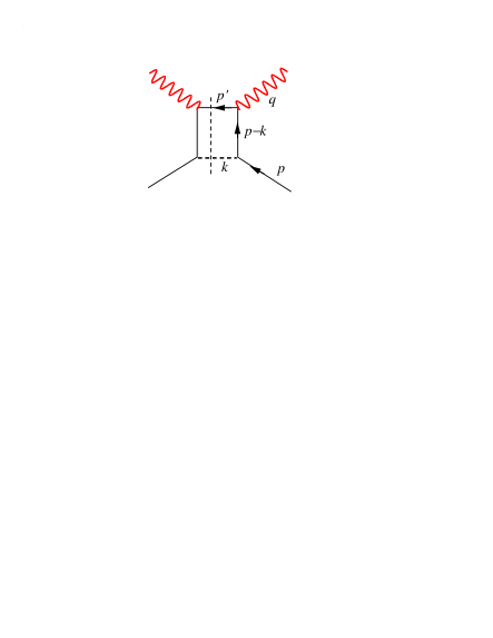
Figure 3: Diagrammatic representation of box diagram, Eq. (3). The lines are as described in Fig. 2.

It is convenient to write the internal integration variables in terms of $s^{\prime}$ and $x^{\prime}$, where

$$s^{\prime} = (p-k+q)^{2}=m^{2}=(p-k)^{2}+Q^{2}\left(\frac{1}{x^{\prime}}-1\right)$$

$$x^{\prime} = \frac{Q^{2}}{2(p-k)\cdot q}=\frac{Q}{2k_{z}+\frac{Q}{x}}\,.$$ (8)

This substitution gives the result

$${\rm Im}T_{2}(s,x,Q^{2})$$

$$\quad=\frac{e^{2}g^{2}\,Q}{16\pi}\int_{x_{-}}^{x_{+}}\frac{dx^{\prime}}{x^{\prime 2}}\frac{(s+\eta^{2})^{-1/2}}{[m^{2}+Q^{2}\left(\frac{1}{x^{\prime}}-1\right)-s^{\prime}]^{2}}\,,\qquad$$ (9)

with

$$\eta=Q\left(1-\frac{1}{2x}\right)\,.$$ (10)

The limits on the $x^{\prime}$ (or $k_{z}$) integration follow from the conservation of energy and the requirement that $k_{\perp}^{2}\geq 0$. The energy relation is

$$\sqrt{\mu^{2}+k_{\perp}^{2}+k_{z}^{2}}+\sqrt{s^{\prime}+k_{\perp}^{2}+(\eta-k_{z})^{2}}=p_{0}\,.$$ (11)

This is a quadradic equation in $k_{z}$, with roots at

$$k^{\pm}_{z}(k_{\perp})=\eta A\pm\sqrt{\left(\frac{\eta^{2}}{s}+1\right)\left(\frac{\Delta}{4s}-k_{\perp}^{2}\right)}\,,$$ (12)

where

$$A = \left(\frac{s-s^{\prime}+\mu^{2}}{2s}\right)$$

$$\Delta = [s-(\sqrt{s^{\prime}}+\mu)^{2}][s-(\sqrt{s^{\prime}}-\mu)^{2}]\,.$$ (13)

The restrictions on $s$ and $s^{\prime}$ insure that both $A$ and $\Delta$ are real and positive. Introducing $k_{z}^{\pm}\equiv k_{z}^{\pm}(0)$, we see that as long as

$$k^{-}_{z}<k_{z}<k^{+}_{z}$$ (14)

there always exists a value of $k_{\perp}^{2}>0$ that satisfies (11) and the integral is nonzero. This determines the limits. The corresponding limits on $x^{\prime}$ are

$$x_{\pm} = \frac{x}{1+(2xk_{z}^{\mp})/Q}$$ (15)

$$= \frac{x}{1+(2x-1)A\mp\frac{x}{sQ}\sqrt{(s+\eta^{2})\Delta}}\,.$$

It is now a starightforward matter to turn the result (9) for the box diagram into an integral equation for the ladder sum. First observe that the single quark pole term is

$${\rm Im}T_{1}(s,x,Q^{2}) = e^{2}\int\frac{d^{3}p^{\prime}}{(2\pi)^{3}2E_{p^{\prime}}}(2\pi)^{4}\delta^{4}(p^{\prime}-p-q)$$ (16)

$$= 2\pi e^{2}\,\delta(s-m^{2})\,,\qquad$$

With this notation the box diagram can be rewritten

$${\rm Im}T_{2}(s,x,Q^{2})=\frac{g^{2}\,Q}{32\pi^{2}}\int_{m^{2}}^{(\sqrt{s}-\mu)^{2}}\!\!\!\!\!\!\frac{ds^{\prime}}{\sqrt{s+\eta^{2}}}\int_{x_{-}}^{x_{+}}\frac{dx^{\prime}}{x^{\prime 2}}\frac{{\rm Im}T_{1}(s^{\prime},x^{\prime},Q^{2})}{[m^{2}+Q^{2}\left(\frac{1}{x^{\prime}}-1\right)-s^{\prime}]^{2}}\,,\qquad$$ (17)

where the upper limit on the $s^{\prime}$ integral follows from the general requirement that $\sqrt{s}\geq\sqrt{s^{\prime}}+\mu$. The integral equation we seek is the immediate generalization of (17):

$${\rm Im}T_{\infty}(s,x,Q^{2})={\rm Im}T_{1}(s,x,Q^{2})+\frac{g^{2}\,Q}{32\pi^{2}}\int_{m^{2}}^{(\sqrt{s}-\mu)^{2}}\!\!\!\!\!\!\frac{ds^{\prime}}{\sqrt{s+\eta^{2}}}\int_{y_{-}}^{y_{+}}\frac{dx^{\prime}}{x^{\prime 2}}\frac{{\rm Im}T_{\infty}(s^{\prime},x^{\prime},Q^{2})}{[m^{2}+Q^{2}\left(\frac{1}{x^{\prime}}-1\right)-s^{\prime}]^{2}}\,,\qquad$$ (18)

It is instructive to cast this equation into an alternative form convenient for solution. To this end, first introduce virtual mass parameters for the external and internal quarks:

$$\kappa = -p^{2}=Q^{2}\left(\frac{1}{x}-1\right)-s$$

$$\kappa^{\prime} = -(p-k)^{2}=Q^{2}\left(\frac{1}{x^{\prime}}-1\right)-s^{\prime}\,.$$ (19)

For simplicity, we also set $\mu=0$. It is then a straightforward matter to transform Eq. (18) into

$${\rm Im}T_{\infty}(s,\kappa,Q^{2})={\rm Im}T_{1}(s,\kappa,Q^{2})+\frac{g^{2}}{16\pi^{2}}\int_{m^{2}}^{s}\!\!\!\!\!\!ds^{\prime}\int_{\kappa^{\prime}_{-}}^{\kappa^{\prime}_{+}}\frac{d\kappa^{\prime}}{\sqrt{\Delta_{0}}}\frac{{\rm Im}T_{\infty}(s^{\prime},\kappa^{\prime},Q^{2})}{[m^{2}+\kappa^{\prime}]^{2}}\,,\qquad$$ (20)

with

$$\kappa^{\prime}_{\pm} = \kappa+\frac{s-s^{\prime}}{2s}\left[Q^{2}+s-\kappa\pm\sqrt{\Delta_{0}}\right]$$

$$\Delta_{0} = s^{2}+\kappa^{2}+Q^{4}-2\kappa Q^{2}+2s\kappa+2sQ^{2}\,,$$ (21)

Finally, introduce new variables

$$x_{B}=\frac{Q^{2}}{s+Q^{2}}\qquad\alpha=\frac{s^{\prime}+Q^{2}}{s+Q^{2}}\,.$$ (22)

In terms of these, Eq. (20) becomes finally

$$M(x_{B},\kappa,Q^{2})-M_{\rm pole}(x_{B},\kappa,Q^{2})=\frac{g^{2}\,Q^{2}}{16\pi^{2}\,x_{B}}\int_{\alpha_{\rm min}}^{1}\!\!\!\!\!\!d\alpha\int_{\kappa_{-}}^{\kappa_{+}}\frac{d\kappa^{\prime}}{\sqrt{\Delta_{0}}}\frac{M(x_{B}/\alpha,\kappa^{\prime},Q^{2})}{[m^{2}+\kappa^{\prime}]^{2}}\,,\qquad$$ (23)

with

$$\alpha_{\rm min} = x_{B}\left(1+\frac{m^{2}}{Q^{2}}\right)$$

$$\kappa_{\pm} = \kappa+\frac{1-\alpha}{2(1-x_{B})}\left[\frac{Q^{2}}{x_{B}}-\kappa\pm\sqrt{\Delta_{0}}\right]$$

$$\Delta_{0} = \left(\kappa+\frac{Q^{2}}{x_{B}}\right)^{2}-4\kappa Q^{2}\,,$$ (24)

with Im$T_{\infty}(s,\kappa,Q^{2})=M(x_{B},\kappa,Q^{2})$, and

$$M_{\rm pole}(x_{B},\kappa,Q^{2})=\frac{2\pi e^{2}x_{B}^{2}}{Q^{2}}\;\delta\left(x_{B}-\frac{Q^{2}}{m^{2}+Q^{2}}\right)\,.$$ (25)

Equation (18) is exact, and Eq. (23) is exact in the $\mu=0$ limit.

III The regge limit

We now apply Eq. (23) to the case of DIS from an off shell quark (neglecting the photon spin until the next section). If the strong coupling $g$ is small, under what circumstances (if any) will the r.h.s. be larger than the pole term, requiring a nonperturbative solution to the equation?

III.1 Approximate equation

The form of the r.h.s. of (23) suggests that it will be large only if $x_{B}$ is small, and hence this term may be approximated by taking $x_{B}$ small. This will be assumed in what follows, and confirmed later, after the approximate solution has been obtained. As $x_{B}\to 0$, the following approximations hold

$$\sqrt{\Delta_{0}} \simeq \frac{Q^{2}}{x_{B}}+\kappa+{\cal O}(x_{B})$$

$$\kappa_{+} \simeq \kappa_{\rm max}+{\cal O}(x_{B})$$

$$\kappa_{-} \simeq \alpha\,\kappa+{\cal O}(x_{B})$$

$$\alpha_{\rm min} \simeq x_{B}+{\cal O}\left(\frac{m^{2}}{Q^{2}}\right)$$

$$\kappa_{\rm max} \equiv Q^{2}\left(\frac{1}{x_{B}}+1\right)(1-\alpha)+\kappa\,.$$ (26)

This gives the following equation, which should hold approximately for all $x_{B}$ and $Q^{2}>\!\!>m^{2}$

$$M(x_{B},\kappa,Q^{2})-M_{\rm pole}(x_{B},\kappa,Q^{2})$$

$$\qquad\quad=\frac{g^{2}}{16\pi^{2}}\int_{x_{B}}^{1}\!\!\!\!\!\!d\alpha\int_{\alpha\kappa}^{\kappa_{\rm max}}\!\!\!d\kappa^{\prime}\;\frac{M(x_{B}/\alpha,\kappa^{\prime},Q^{2})}{[m^{2}+\kappa^{\prime}]^{2}}\,.\qquad$$ (27)

We emphasize that this equation differs from the exact Eq. (23) only in the form of r.h.s., which by assumption is large only at small $x_{B}$ where the approximate form used in (27) is accurate.

III.2 Approximate solution for small $x_{B}$

Following Ref. Simonov , assume that $M$ exhibits a Regge-like behavior at small $x_{B}$

$$M(x_{B},\kappa,Q^{2})\big{|}_{{\rm small}\,x_{B}}\simeq\left(\frac{1}{x_{B}}\right)^{\ell}R(x_{B},\kappa,Q^{2})\,,$$ (28)

where $R$ is finite as $x_{B}\to 0$. The power $\ell$ will be determined self consistently from the equation. Substituting this anzatz into (27), and neglecting the inhomogeneous pole term which is small at small $x_{B}$, gives an equation for $R(x_{B},\kappa,Q^{2})$

$$R(x_{B},\kappa,Q^{2})$$

$$\quad=\frac{g^{2}}{16\pi^{2}}\int_{x_{B}}^{1}\!\!\!\!\!\!d\alpha\,\alpha^{\ell}\int_{\alpha\kappa}^{\kappa_{\rm max}}\!\!\!d\kappa^{\prime}\;\frac{R(x_{B}/\alpha,\kappa^{\prime},Q^{2})}{[m^{2}+\kappa^{\prime}]^{2}}\,,\qquad$$ (29)

where, by assumption, $R(0,\kappa,Q^{2})$ is finite. This quantity satisfies the equation

$$R(0,\kappa,Q^{2}) = \lambda\,m^{2}\int_{0}^{1}d\alpha\,\alpha^{\ell}\int_{\alpha\kappa}^{\infty}\!d\kappa^{\prime}\;\frac{R(0,\kappa^{\prime},Q^{2})}{[m^{2}+\kappa^{\prime}]^{2}}\,,$$ (30)

$$= \frac{\lambda\,m^{2}}{(\ell+1)}\Bigg{\{}\int_{\kappa}^{\infty}\!d\kappa^{\prime}+\int_{0}^{\kappa}d\kappa^{\prime}\left(\frac{\kappa^{\prime}}{\kappa}\right)^{\ell+1}\Bigg{\}}\,\frac{R(0,\kappa^{\prime},Q^{2})}{[m^{2}+\kappa^{\prime}]^{2}}\,,\qquad$$

where $\lambda=g^{2}/(16\pi^{2}m^{2})$ is dimensionless. Note that $R(0,\kappa,Q^{2})$ is independent of $Q^{2}$. The boundary conditions on $R$ are $R\to 0$ as $\kappa\to\infty$, and $R(0,0,Q^{2})=$ constant. Introducing the dimensionless variables $y=\kappa/m^{2}$ and $y^{\prime}=\kappa^{\prime}/m^{2}$, and differentiating the equation by $y$ twice, leads to a differential equation for $r(y)\equiv R(0,\kappa,Q^{2})$

$$y\,r^{\prime\prime}+(\ell+2)r^{\prime}+{\lambda\over(y+1)^{2}}\ r=0.$$ (31)

The general solution of this equation is a hypergeometric function AS

$$r(y)\propto F\left(a,b,c,\frac{y}{1+y}\right)$$ (32)

with

$$a = \frac{1}{2}-\frac{1}{2}\sqrt{1+4\lambda}$$

$$b = \frac{1}{2}+\frac{1}{2}\sqrt{1+4\lambda}$$

$$c = \ell+2\,.$$ (33)

The value of $\ell$ is fixed by the $y\to\infty$ boundary condition, which requires that the hypergeometric function approach zero as $z\equiv y/(1+y)\to 1$. First, the hypergeometric series will not converge at $z=1$ unless $c-a-b>0$, and this requires $\ell+1>0$. Then, using the properties of the hypergeometric function AS , we have

$$F(a,b,c,1)=\frac{\Gamma(c)\Gamma(c-a-b)}{\Gamma(c-a)\Gamma(c-b)}$$

$$=\frac{\Gamma(\ell+2)\Gamma(\ell+1)}{\Gamma(\ell+\frac{3}{2}+\frac{1}{2}\sqrt{1+4\lambda})\Gamma(\ell+\frac{3}{2}-\frac{1}{2}\sqrt{1+4\lambda})}\,.\qquad$$ (34)

This can be zero if and only if the arguments of one of the $\Gamma$ functions in the denominator is $-n$, where $n$ is zero or a positive integer. Since $\ell+1>0$, it must be the argument of the second $\Gamma$ function that is $-n$, and hence the only possible values of $\ell$ are

$$\ell=\ell_{n}\equiv\frac{1}{2}\left(\sqrt{1+4\lambda}-3-2n\right)\quad n=(0,1,2,\cdots)\,.\quad$$ (35)

The requirement $\ell+1>0$ yields

$$\lambda=\frac{(2\ell+3+2n)^{2}-1}{4}>0\,,$$ (36)

so there are solutions even if $\lambda$ is very small, as anticipated. The solutions for $n=0$ were previously obtained in Ref. Simonov .

For large $\lambda$ there will be more than one value of $\ell$ that satisfies the condition (35). The number of values depends on the size of $\lambda$. Specifically,

$$\begin{array}[]{ll}\ell=\ell_{0}\equiv\frac{1}{2}\left(\sqrt{1+4\lambda}-3\right)&{\rm if}\;\phantom{1}2>\lambda>0\cr&\cr\ell=\ell_{0}\;{\rm or}\;\ell_{1}&{\rm if}\;\phantom{1}6>\lambda>2\cr&\cr\ell=\{\ell_{0},\ell_{1},\ell_{2}\}&{\rm if}\;12>\lambda>6\cr\cdots&\end{array}$$ (43)

For $\lambda>2$ the general small $x_{B}$ solution will be a sum of contributions from the different trajectories

$$M(x_{B},\kappa,Q^{2})\big{|}_{{\rm small}\,x_{B}}=\sum_{n=0}^{n_{\rm max}}c_{n}\left(\frac{1}{x_{B}}\right)^{\ell_{n}}\!\!\!r_{n}\left(\frac{\kappa}{m^{2}}\right)\,.$$ (44)

The solution $r_{0}(y)$ for the “leading” trajectory, $n=0$, is

$$r_{0}(y) = F(a,b,b,z)=\left(\frac{1}{1-z}\right)^{a}=\left(\frac{m^{2}}{m^{2}+\kappa}\right)^{\ell_{0}+1}\qquad$$ (45)

For small $\lambda$ (i.e. $\lambda<2$) there is only one trajectory, and we obtain the unique approximation

$$M_{0}(x_{B},\kappa,Q^{2})=c_{0}\left(\frac{1}{x_{B}}\right)^{\ell_{0}}\!\!\!\left(\frac{m^{2}}{m^{2}+\kappa}\right)^{\ell_{0}+1}\!\!\!,\quad$$ (46)

with $c_{0}$ an undetermined coefficient.

Some additional arguments which demonstrate that we have found all of the solutions are given in Appendix A

At this point we are left with several unanswered questions: (i) How is the coefficient $c_{0}$ to be fixed? (ii) Only the leading dependence at small $x_{B}$ is given by $M_{0}$. How large are the nonleading terms at small $x_{B}$ and what is their analytic form? (iii) How is the pole term to be included in the solution and how is the large $x_{B}$ dependence described approximately?

All of these questions will be answered in the following subsection. It turns out that substitution of the ansatz

$$M(x_{B},\kappa,Q^{2})=M_{\rm pole}(x_{B},\kappa,Q^{2})+M_{0}(x_{B},\kappa,Q^{2})\,,\qquad$$ (47)

into Eq. (27) will show how to fix the coefficient $c_{0}$ so that (47) will give a satisfactory solution to (27) for all $x_{B}$.

III.3 Approximate solution for all $x_{B}$

Substituting $M_{0}$ into the r.h.s. of the asymptotic Eq. (27) gives

$${\rm r.h.s.} = c_{0}\lambda\,m^{2}\int_{x_{B}}^{1}\!\!\!\!\!\!d\alpha\left(\frac{\alpha}{x_{B}}\right)^{\ell_{0}}\int_{\alpha\kappa}^{\kappa_{\rm max}}\!\!\!d\kappa^{\prime}\;\frac{m^{2\ell_{0}+2}}{[m^{2}+\kappa^{\prime}]^{\ell_{0}+3}}\qquad$$ (48)

$$= \frac{c_{0}\lambda}{(\ell_{0}+2)}\int_{x_{B}}^{1}\!\!\!\!d\alpha\left(\frac{\alpha}{x_{B}}\right)^{\ell_{0}}\Bigg{\{}\left(\frac{m^{2}}{m^{2}+\alpha\kappa}\right)^{\ell_{0}+2}-\left(\frac{m^{2}}{m^{2}+\kappa_{\rm max}}\right)^{\ell_{0}+2}\Bigg{\}}\,.$$

The first term is the leading term, and doing the $\alpha$ integration gives

$${\rm r.h.s.}\big{|}_{\rm 1st} = \frac{c_{0}\lambda}{(\ell_{0}+2)(\ell_{0}+1)}\Bigg{\{}\frac{1}{x_{B}^{\ell_{0}}}\left(\frac{m^{2}}{m^{2}+\kappa}\right)^{\ell_{0}+1}-x_{B}\left(\frac{m^{2}}{m^{2}+x_{B}\kappa}\right)^{\ell_{0}+1}\Bigg{\}}\quad$$ (49)

$$= M_{0}(x_{B},\kappa,Q^{2})-c_{0}\;x_{B}\left(\frac{m^{2}}{m^{2}+x_{B}\kappa}\right)^{\ell_{0}+1}\,.$$

This shows that $M_{0}$ is a solution of the homogeneous equation with an error [the second term in (49)] which vanishes linearly as $x_{B}\to 0$, showing that $M_{0}$ is accurate to ${\cal O}(x_{B}^{1+\ell_{0}})$. This is not very satisfactory, particularly when $\lambda$ is small and $\ell_{0}\to-1$. The pole term, not yet discussed, will correct this problem. The second term in (48) gives a correction proportional to $m^{2}x_{B}/Q^{2}$. At large $Q^{2}$ it becomes

$$\lim_{Q^{2}\to\infty}{\rm r.h.s.}\big{|}_{\rm 2nd} \to \bigg{[}M_{0}(x_{B},\kappa,Q^{2})-c_{0}\left(\frac{m^{2}x_{B}^{2}}{(m^{2}+\kappa)\,x_{B}+Q^{2}(1-x_{B}^{2})}\right)^{\ell_{0}+1}\bigg{]}\frac{m^{2}x_{B}}{Q^{2}(1+x_{B})}\,.$$ (50)

In applications to DIS, these terms can safely be neglected.

Next, we look at the effect of inserting the pole term (25) into the r.h.s. of (27). This gives

$${\rm r.h.s.}\big{|}_{\rm pole} = \frac{2\pi\lambda\,e^{2}\,x_{B}^{2}}{Q^{2}}\int_{x_{B}}^{1}\!\!\frac{d\alpha}{\alpha^{2}}\;\delta\left(\frac{x_{B}}{\alpha}-\frac{Q^{2}}{m^{2}+Q^{2}}\right)\int_{\alpha\kappa}^{\kappa_{\rm max}}\!\!\!d\kappa^{\prime}\;\frac{m^{2}}{[m^{2}+\kappa^{\prime}]^{2}}\qquad$$ (51)

$$\simeq \frac{2\pi\lambda\,e^{2}\,x_{B}}{Q^{2}}\Bigg{\{}\frac{m^{2}}{m^{2}+x_{B}\kappa}-\frac{m^{2}x_{B}}{(m^{2}+\kappa)\,x_{B}+Q^{2}(1-x_{B}^{2})}\Bigg{\}}\,,$$

where we assumed that $Q^{2}>\!\!>m^{2}$ so that the delta function gives $\alpha=x_{B}$. The second term is small at large $Q^{2}$ (except at the exceptional point $x_{B}=1$). Combining the first term in (51) with the correction term in (49) gives

$${\rm r.h.s.}\big{|}_{{\rm pole}+{\rm corr}} = \frac{2\pi\lambda\,e^{2}\,x_{B}}{Q^{2}}\left(\frac{m^{2}}{m^{2}+x_{B}\kappa}\right)-c_{0}\;x_{B}\left(\frac{m^{2}}{m^{2}+x_{B}\kappa}\right)^{\ell_{0}+1}$$ (52)

$$\simeq x_{B}\;\left[\frac{2\pi\lambda\,e^{2}}{Q^{2}}-c_{0}\right]-x_{B}^{2}\;\left[\frac{2\pi\lambda\,e^{2}}{Q^{2}}-(\ell_{0}+1)\,c_{0}\right]\frac{\kappa}{m^{2}}+\cdots\,,$$

Setting

$$c_{0}=\frac{2\pi\lambda\,e^{2}}{Q^{2}}$$ (53)

will cancel the leading error term and insure that the ansatz (47) is accurate to ${\cal O}(x_{B}^{2+\ell_{0}})$ and vanishes as $x_{B}\to 0$ for all $\ell_{0}$. We conclude that the solution (47) with the choice (53) is accurate for all $x_{B}$ and $Q^{2}$ as long as $Q^{2}>\!\!>m^{2}$.

III.4 Summation of the series for small $x_{B}$ and $\kappa$

Before leaving this discussion, it is instructive to show explicitly how the Regge behavior (46) arises by summing the infinite number of terms in the series defined by the iteration of Eq. (27).

Iteration of Eq. (27) generates the following series:

$$M(x_{B},\kappa,Q^{2})-M_{\rm pole}(x_{B},\kappa,Q^{2})$$

$$\qquad\qquad\qquad=\sum_{n=0}^{\infty}M^{(n+1)}(x_{B},\kappa,Q^{2})$$ (54)

where, taking $\kappa_{\rm max}\to\infty$,

$$M^{(n+1)}(x_{B},\kappa,Q^{2})=\int_{\alpha,\kappa^{\prime}}\frac{M^{(n)}(x_{B}/\alpha,\kappa^{\prime},Q^{2})}{[m^{2}+\kappa^{\prime}]^{2}}\,,$$ (55)

with

$$M^{(0)}(x_{B},\kappa,Q^{2})\equiv M_{\rm pole}(x_{B},\kappa,Q^{2})$$ (56)

and

$$\int_{\alpha,\kappa^{\prime}}\equiv\frac{g^{2}}{16\pi^{2}}\int_{x_{B}}^{1}\!\!\!\!\!\!d\alpha\int_{\alpha\kappa}^{\infty}\!\!\!d\kappa^{\prime}\,.$$ (57)

Near $\kappa=0$, the leading $\log(x_{B})$ terms in this series can be summed. In Appendix B we show that these leading terms are given by the simpler series

$$M^{(n+1)}_{\rm leading}(x_{B})=\lambda\int_{x_{B}}^{1}d\alpha\;M^{(n)}_{\rm leading}(x_{B}/\alpha)\,.$$ (58)

With the aid of the identity

$$\int_{1}^{1/x_{B}}\frac{dy}{y}\log^{n}(y)=\frac{1}{n+1}\log^{n+1}\left(\frac{1}{x_{B}}\right)\,,$$ (59)

the general term becomes

$$M^{(n+1)}_{\rm leading}(x_{B})=\frac{c_{0}x_{B}}{n!}\left[\lambda\log\left(\frac{1}{x_{B}}\right)\right]^{n}\,,$$ (60)

and summing to all orders gives

$$c_{0}x_{B}\sum_{n=0}^{\infty}\frac{1}{n!}\left[\lambda\log\left(\frac{1}{x_{B}}\right)\right]^{n}=c_{0}x_{B}\left(\frac{1}{x_{B}}\right)^{\lambda}$$ (61)

in precise agreement with the small $\lambda$ and small $\kappa$ limit of (46) (where $\ell_{0}\simeq-1+\lambda$).

This calculation confirms the normalization the solution, but it also shows explicitly that the Regge behavior arises when $\lambda\log x_{B}\sim-1$, the condition that insures that all of the loops are of comparable size. Under these conditions perturbation theory breaks down and a nonperturbative summation of all diagrams is needed.

IV dis structure functions

In this section the results of the previous section are applied to DIS. First we add the photon vector degrees of freedom, then we compute the two diagrams shown in Fig. 1.

IV.1 Photon degrees of freedom

The vector degrees of freedom of the photon will introduce additional structure into the pole term (25) and the scattering amplitude (47). The pole term becomes

$$J_{\rm pole}^{\mu\nu}(x_{B},p,Q)$$

$$\qquad=(2p-q)^{\mu}(2p-q)^{\nu}M_{\rm pole}(x_{B},-p^{2},Q^{2})\,.\qquad\quad$$ (62)

If both the initial and final quarks were on-shell, this would be gauge invariant, but the initial quark is not on-shell. We impose gauge invariance in the manner suggested in Ref. BG1 , where it was found that the substitution

$$J^{\mu}\to J^{\mu}-\frac{J\cdot q\;q^{\mu}}{q^{2}}$$ (63)

insured that the final state interactions vanished in the DIS limit. This choice therefore preserves the dominance of the pole term in the DIS limit, and is what is needed in the absence of a full theory. Applied to the product of two currents, it leads to the replacement

$$J^{\mu\nu} \to J^{\mu\nu}-\frac{(J^{\mu\nu^{\prime}}q_{\nu^{\prime}})\;q^{\nu}}{q^{2}}-\frac{(J^{\mu^{\prime}\nu}q_{\mu^{\prime}})\;q^{\mu}}{q^{2}}$$ (64)

$$+\frac{(J^{\mu^{\prime}\nu^{\prime}}q_{\mu^{\prime}}q_{\nu^{\prime}})\;q^{\mu}q^{\nu}}{q^{4}}\,.$$

This, in turn, give the substitutions

$$g^{\mu\nu}\to g^{\mu\nu}-\frac{q^{\mu}\,q^{\nu}}{q^{2}}\equiv\tilde{g}^{\mu\nu}$$

$$p^{\mu}p^{\nu}\to\left(p^{\mu}-\frac{p\cdot q\,q^{\mu}}{q^{2}}\right)\left(p^{\nu}-\frac{p\cdot q\,q^{\nu}}{q^{2}}\right)\equiv\tilde{p}^{\mu}\tilde{p}^{\nu}$$

$$q^{\mu}q^{\nu}\to 0$$

$$p^{\mu}q^{\nu}+q^{\mu}p^{\nu}\to 0\,,$$ (65)

and the pole term (62) is transformed into the familiar form

$$J_{\rm pole}^{\mu\nu}(x_{B},p,Q)=4\tilde{p}^{\mu}\tilde{p}^{\nu}M_{\rm pole}(x_{B},\kappa,Q^{2})\,,\qquad\quad$$ (66)

where, as before, $\kappa=-p^{2}$. The general structure of the full amplitude will be expressed in term of two scalar functions

$$J^{\mu\nu}(x_{B},p,Q)= - \tilde{g}^{\mu\nu}\;w_{1}(x_{B},\kappa,Q^{2})$$ (67)

$$+ \frac{\tilde{p}^{\mu}\tilde{p}^{\nu}}{\tilde{p}^{2}}\;w_{2}(x_{B},\kappa,Q^{2})\,,\qquad$$

where the $w_{i}$ differ from the familiar $W_{i}$ of DIS by normalization and the dependence on the off-shell quark mass.

When the form (67) is inserted into the integral that leads eventually to Eq. (23) or (27), the integration over the azymuthal angle $\pi$, which was originally trivial, now requires use of the identity

$$\frac{1}{2\pi}\int_{0}^{2\pi}d\phi\;(\tilde{p}-\tilde{k})^{\mu}(\tilde{p}-\tilde{k})^{\nu}$$

$$\qquad\to-\frac{1}{2}k_{\perp}^{2}\tilde{g}^{\mu\nu}+\frac{\tilde{p}^{\mu}\tilde{p}^{\nu}}{\tilde{p}^{2}}\left(\frac{1}{2}k_{\perp}^{2}+(p_{0}-k_{0})^{2}\right)\,.\qquad$$ (68)

The quantities in this equation can be expressed in terms of the variables used in Eq. (27). In the small $x_{B}$, large $Q^{2}$ limit

$$k_{\perp}^{2}\to(1-\alpha)\,(\kappa^{\prime}-\alpha\kappa)$$

$$\tilde{p}^{2}=p_{0}^{2}\to\frac{Q^{2}}{4x_{B}^{2}}$$

$$\frac{1}{2}k_{\perp}^{2}+(p_{0}-k_{0})^{2}\to\frac{\alpha^{2}Q^{2}}{4x_{B}^{2}}$$

$$(\tilde{p}-\tilde{k})^{2}\to\frac{\alpha^{2}Q^{2}}{4x_{B}^{2}}$$ (69)

Hence Eq. (27) generalizes to a system of coupled equations for the $w_{i}$

$$w_{1}(x_{B},\kappa,Q^{2})=\frac{g^{2}}{16\pi^{2}}\int_{x_{B}}^{1}\!\!\!\!\!\!d\alpha\int_{\alpha\kappa}^{\kappa_{\rm max}}\!\!\!\frac{d\kappa^{\prime}}{[m^{2}+\kappa^{\prime}]^{2}}\Big{\{}\frac{2x_{B}^{2}\,(1-\alpha)\,(\kappa^{\prime}-\alpha\kappa)}{\alpha^{2}Q^{2}}\,w_{2}(x_{B}/\alpha,\kappa^{\prime},Q^{2})+w_{1}(x_{B}/\alpha,\kappa^{\prime},Q^{2})\Big{\}}$$

$$w_{2}(x_{B},\kappa,Q^{2})-4\tilde{p}^{2}M_{\rm pole}(x_{B},\kappa,Q^{2})=\frac{g^{2}}{16\pi^{2}}\int_{x_{B}}^{1}\!\!\!\!d\alpha\int_{\alpha\kappa}^{\kappa_{\rm max}}\!\!\!d\kappa^{\prime}\;\frac{w_{2}(x_{B}/\alpha,\kappa^{\prime},Q^{2})}{[m^{2}+\kappa^{\prime}]^{2}}\,.\qquad$$ (70)

Note that the equation for $w_{2}$ is identical to (27) except for the factor of $4\tilde{p}^{2}$ multiplying the pole term, and that $w_{1}$ is smaller than $w_{2}$ by $Q^{-2}$, and can be ignored. The factor of $4\tilde{p}^{2}$ changes the value of $c_{0}$ extracted from the cancellation described in Eq. (52), but otherwise does not alter the argument. Incorporating these modifications into the solution obtained in the previous section, and taking the high $Q^{2}$ limit, gives

$$w_{1}(x_{B},\kappa,Q^{2}) \to 0$$

$$w_{2}(x_{B},\kappa,Q^{2}) = 2\pi e^{2}\,\delta(x_{B}-1)$$ (71)

$$+\frac{e^{2}g^{2}}{8\pi m^{2}}\left(\frac{1}{x_{B}}\right)^{\ell_{0}}\!\!\!\left(\frac{m^{2}}{m^{2}+\kappa}\right)^{\ell_{0}+1}\!\!\!\!\!\!.\qquad$$

Note that this solution is dimensionless and independent of $Q^{2}$.

IV.2 Structure function for scalar bound states

We now use the result (71) to construct the contributions from each of the diagrams shown in Fig. 1. Figure 4 shows the labeling of momenta in the generic convolution diagram. In this part of the calculation we choose a different coordinate system, with momenta

$$P = \{M_{B},{\bf 0},0\}$$

$$P_{Q} = \{{\cal E},-{\bf p}_{\perp},-p_{3}\}$$

$$q = \{\nu,{\bf 0},q_{{}_{L}}\}$$

$$p = \{M_{B}-{\cal E},{\bf p}_{\perp},p_{3}\}\,,$$ (72)

where ${\cal E}=\sqrt{M^{2}+p^{2}_{\perp}+p_{3}^{2}}$ as required by the condition that the heavy quark is on its positive energy mass-shell. Since the off-shell quark structure function $w_{2}$ is manifestly covariant, it may be written in any coordinate system, and we will use this property to write it in the coordinate system defined by the choices given in Eq. (72). With this choice the variable $x$ takes on the familiar form

$$x=\frac{Q^{2}}{2M_{B}\nu}\,.$$ (73)

In the covariant spectator formalismgross , the diagram in Fig. 4 is

$$J_{B}^{\mu\nu}(P,q) = \int\frac{d\phi\,dp_{\perp}^{2}dp_{3}}{(2\pi)^{3}4{\cal E}}\;\Psi^{2}(p^{2})\,J^{\mu\nu}(x_{B},p,q)$$ (74)

$$\equiv \int d\Sigma\;J^{\mu\nu}(x_{B},p,q)$$

where $J^{\mu\nu}$ was defined in Eq. (67) and

$$\Psi(p^{2})=\frac{\Gamma(p^{2})}{m^{2}-p^{2}}$$ (75)

is the relativistic wave function (by definition), with $\Gamma(p^{2})$ the covariant vertex function for the coupling of a bound meson with mass $M_{B}$ to an on-shell heavy quark with mass $M$ and an off-shell light quark with four-momentum $p$. In the scalar theory we are describing this can be a function of $p^{2}$ only.

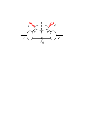
Figure 4: Diagram showing the convolution of the scattering amplitude $w_{2}$ from Eq. (71) with the covariant bound state vertex function, as canculated in the spectator theory. The on-shell heavy quark is labeled by an $\times$ in the diagram.

Decomposing (74) into the standard scalar functions

$$J^{\mu\nu}_{B}(P,q)=-W_{1}(\nu,Q^{2})\,\tilde{g}^{\mu\nu}+W_{2}(\nu,Q^{2})\frac{\tilde{P}^{\mu}\tilde{P}^{\nu}}{M_{B}^{2}}\,,$$ (76)

multiplying by $g_{\mu\nu}$ and $P_{\mu}P_{\nu}$, and separating $W_{1}$ and $W_{2}$, gives the following expressions

$$\left(1+\frac{\nu}{2M_{B}x}\right)W_{2}(\nu,Q^{2})=\frac{1}{2}\int d\Sigma\;w_{2}\left[3\,\theta-1\right]$$

$$W_{1}(\nu,Q^{2})=\int d\Sigma\;\bigg{\{}w_{1}+\frac{1}{2}w_{2}\left[\theta-1\right]\bigg{\}}\,,\qquad$$ (77)

with

$$w_{i} = w_{i}(x_{B},-p^{2},Q^{2})$$

$$\theta = \theta(p_{\perp}^{2},p_{3})=\frac{(P\cdot\tilde{p})^{2}}{\tilde{p}^{2}M_{B}^{2}\left(1+\frac{\nu}{2M_{B}x}\right)}\,,$$ (78)

and we retained $w_{1}$ for completeness. In the high $Q^{2}$ limit, $q_{{}_{L}}\sim\nu\sim Q^{2}$, and $P\cdot\tilde{p}\to(P\cdot q)(p\cdot q)/Q^{2}$ and $\tilde{p}^{2}\to(p\cdot q)^{2}/Q^{2}$ giving

$$\lim_{Q^{2}\to\infty}\theta(p_{\perp}^{2},p_{3})\to 1\,.$$ (79)

Hence $W_{1}$ vanishes (as expected for scalar constituents), and, as $Q^{2}\to\infty$,

$$\nu W_{2}(\nu,Q^{2})\to 2M_{B}x\int\frac{\,dp_{\perp}^{2}dp_{3}}{(2\pi)^{2}4{\cal E}}\;\Psi^{2}(p^{2})\,w_{2}$$ (80)

The integral (80) is best expressed in terms of the independent variables $p_{\perp}^{2}$ and $p_{-}$. Introducing the dimensionless variable $z=p_{-}/M_{B}$, so that

$$-p^{2} = \frac{1}{1-z}\left(p_{\perp}^{2}+zM^{2}-z(1-z)M_{B}^{2}\right)$$

$$x_{B} = \frac{Q^{2}}{s+Q^{2}}\to\frac{x}{z}\;\;\mbox{(at large $Q^{2}$)}\,,$$ (81)

and introducing the constant

$$S_{0}=m^{2}M_{B}\frac{e^{2}}{4\pi}$$ (82)

gives

$$\nu W_{2}(\nu,Q^{2}) = x\,S_{0}\int_{0}^{\infty}\frac{dp_{\perp}^{2}}{m^{2}}\int_{x}^{1}\frac{dz}{1-z}\;\Psi^{2}(p^{2})\left[\delta\left(\frac{x}{z}-1\right)+\lambda\left(\frac{z}{x}\right)^{\ell_{0}}\left(\frac{m^{2}}{m^{2}-p^{2}}\right)^{\ell_{0}+1}\right]\,.$$ (83)

Note that $\nu W_{2}$ goes like $x^{1-\ell_{0}}$ at small $x$, as it is expected on general grounds [1-4].

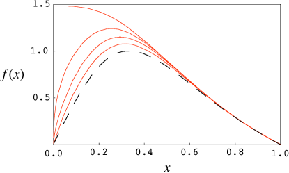
Figure 5: The structure function $f(x)=\nu W_{2}/x$ as a function of $x$ for the model discussed in the text. The solid lines are the sum of the pole and the Regge contributions for values of $\lambda=0.2,0.5,1.0$ and $2.0$, with the curves increasing in value as $\lambda$ increases. The dashed line is the pole contribution, which is independent of $\lambda$ in our simple approximation.

It is instructive and amusing to evaluate $\nu W_{2}$ for a simple model, and look at the comparative behavor of the two terms. A detailed study would require the solution of the bound state spectator equation for the spectator wave function. While this is not difficult, it is also not necessary in order to obtain a qualitative understanding of the physics. To this end we introduce a very simple ansatz for the wave function

$$\Psi(p^{2}) = \left(\frac{m^{2}}{m^{2}-p^{2}}\right)^{\beta}$$ (84)

$$= (1-z)^{\beta}\left(\frac{m^{2}}{{\cal M}^{2}(z)+p_{\perp}^{2}}\right)^{\beta}$$

with

$${\cal M}^{2}(z)=(1-z)\,m^{2}+z\,M^{2}-z(1-z)M_{B}^{2}$$ (85)

In the following example we take $\beta=1$ for simplicity.

We now evaluate each of the terms in (83). The first term is the pole contribution, shown in Fig. 1(a). Immediate evaluation of the $z$ integral gives

$$\nu W_{2}\Big{|}_{\rm pole}=S_{0}\,\frac{x^{2}}{1-x}\int_{0}^{\infty}\frac{dp_{\perp}^{2}}{m^{2}}\;\Psi^{2}(p^{2}(z=x))\,,$$ (86)

and evaluating the $p_{\perp}$ integral gives

$$\nu W_{2}\Big{|}_{\rm pole}=\frac{S_{0}\,x^{2}\,(1-x)}{1-x+x\,M_{0}^{2}-x(1-x)M_{B0}^{2}}\,.$$ (87)

This function is shown (as a dashed line) in Fig. 5, for the choices $M_{0}\equiv M/m=2$, $M_{B0}\equiv M_{B}/m=2$, and $S_{0}=10$. It gives the familar shape anticipated in the drawing shown in Fig. 1; it is zero at the $x=0$ and $x=1$ boundaries.

The new result of this paper is the inclusion of the small $x$ Regge term with a normalization consistent with the valance contribution. For the model (84) this term becomes

$$\nu W_{2}\Big{|}_{\rm Regge}=\lambda\left(\frac{1}{x}\right)^{\ell_{0}-1}G(x,\lambda)$$ (88)

with

$$G(x,\lambda)=\frac{S_{0}}{\ell_{0}+2}\int_{x}^{1}dz\,z^{\ell_{0}}\left(\frac{m^{2}(1-z)}{{\cal M}^{2}(z)}\right)^{\ell_{0}+2}$$ (89)

where the power $\ell_{0}$ was given in Eq. (LABEL:l0sol). [Note that Eq. (88) agrees with the general result of Eq. (2).] Since $1-\ell_{0}\leq 2$, the Regge term is always larger than the pole term near $x=0$, but the importance of this term depends on the size of $\lambda$. If $\ell_{0}>0$ ($\lambda>2$) the Regge contribution to the quark distribution $f(x)=\nu W_{2}/x$ is singular as $x\to 0$, and the structure function has the shape shown in Fig. 1. But, even for small values of $\lambda$, Fig. 5 shows that the Regge term enhances the distribution significantly.

V conclusions

This paper applies the Regge concepts originally developed in Ref. Simonov to DIS. We find that an approximate solution can be obtained that can explain, qualitatively at least, the enhancement of the structure function at small $x$. The physics that produces this effect is the inelastic production of any number of massless gluons when $x$ is small, and $s$ is corresponding large.

We emphasize that this calculation shows that, even when the strong coupling is small, so that perturbation theory should apply over most of the phase space, there are regions when an an infinite number of diagrams must be summed to get the correct result. The need to do this for the description of bound states is familar to most physicists. Here we have discussed it is also necessary in the small $x$ region when the production of massless gluons must be summed to all orders to give the correct result.

The scalar theory examined in this paper gives an unrealistically small result $\ell(0)\simeq-1+\lambda$ for the $t=0$ intercept of the Regge trajectory. A realistic treatment based on QCD, including spin and confinement, should give an intercept of $\ell(0)=1/2$, corresponding to the $\rho$ trajectory (the largest trajectory possible for a $q\bar{q}$ ladder). While this result could be mimicked in this model by choosing $\lambda=3.75$, this is too large to be realistic, and the failure is due to the physics missing from the scalar theory.

The gluon distribution, which corresponds to $\ell(0)\simeq 1$, is expected to arise from single and multiple pomeron exchanges Kaidalov , mechanisms not included in the model discussed here. The calculation of ladder exchanges of massless gluons of spin one is known to give an intercept around one for small coupling constant, in agreement with the small $x$ behavior of structure functions.

There are many interesting issues and unsolved problems yet to be dealt with. The very notion of Regge trajectories $\alpha_{i}(t)$ in QCD is understood to some extent only for positive $t$ Kaidalov , where it has been shown that the trajectories are indeed linear and the intercepts $\alpha_{i}(0)=\ell_{i}(0)$ have been explicitly calculated theoretically Badalian . At the same time, the behavior of $\alpha_{i}(t)$ for $t<0$ in QCD (and other field theory models) is still unknown, though very interesting from both experimental and theoretical point of view.

As trajectories for $t<0$ are understood, it will be of interest to apply these ideas to other processes, such as exclusive DIS and Virtual Compton Scattering, where $t\neq 0$ and $Q^{2}\neq{Q^{\prime}}^{2}$. Such applications will yield models for the interesting Generalized Parton Distributions (GPDs). Another point of interest is the interconnection of Regge behavior and the DGLAP evolution of structure functions. All of this will require an explicit understanding of the behavior of the Regge trajectories at both positive and negative values of $t$. To obtain linear Regge trajectories with realistic intercepts, and to describe structure functions quanitatively in the whole $x$ region, one needs to modify the ladder kernel of the equations used in this paper to include the nonperturbative effects arising from confinement. Study of these fundamental and difficult problems is planned for future work.

Appendix A

In this appendix we give an alternative demonstration that study of Eq. (29) near $x=0$ will not produce solutions that have not already been considered.

Rewrite Eq. (29)

$$r(y,x)=\lambda\int\limits_{x}^{1}d\alpha\ \alpha^{l}\int\limits_{y\alpha}^{\infty}dy^{\prime}{r(y^{\prime},{x/\alpha})\over(y^{\prime}+1)^{2}}.$$ (90)

where use the fact that the upper limit of the $y^{\prime}$ integration can be taken to infinity with errors that vanish as $Q^{2}\to\infty$.

To simplify the form of the integral in this equation, let us define a new function $\phi(y,x)$ trough

$$r(y,x)=\phi(y,x)(y+1)^{2}x^{l+1}.$$ (91)

The equation for $\phi$

$$\phi(y,x)(y+1)^{2}=\lambda\int\limits_{x}^{1}{d\alpha\over\alpha}\int\limits_{y\alpha}^{\infty}dy^{\prime}\phi\left(y^{\prime},{x\over\alpha}\right)$$ (92)

may be converted to a partial derivative equation through the following steps.

First, after taking $y$- derivative from both sides in Eq.(92), we obtain

$${\partial\left(\phi(y,x)(y+1)^{2}\right)\over\partial y}=-\lambda\int\limits_{x}^{1}d\alpha\phi\left(y\alpha,{x\over\alpha}\right).$$ (93)

Changing the integration variable from $\alpha$ to $z={\alpha\over x}$, we write Eq.(93) as

$$\Phi_{y}={\partial\over\partial y}\left(\phi(y,x)(y+1)^{2}\right)=-\lambda x\int\limits_{1}^{1/x}dz\phi\left(xyz,{1\over z}\right),$$ (94)

where the notations

$$\Phi=\phi(y,x)(y+1)^{2}=r(y,x)x^{-(l+1)},\ \ \ \Phi_{y}\equiv{\partial\over\partial y}\Phi$$

are used.

For partial $x$ and $y$ – derivatives of $\Phi_{y}$ Eq.(94), we have

$$\Phi_{y,x} \equiv {\partial\over\partial x}\Phi_{y}={1\over x}\Phi_{y}-\left(-{1\over x^{2}}\right)\lambda x\phi(y,x)-\lambda x\int\limits_{1}^{1/x}dz\ yz\left.\left({\partial\phi\left(\xi,{1\over z}\right)\over\partial\xi}\right)\right|_{\xi=xyz},$$ (95)

$$\Phi_{y,y} \equiv {\partial\over\partial y}\Phi_{y}=-\lambda x\int\limits_{1}^{1/x}dz\ xz\left.\left({\partial\phi\left(\xi,{1\over z}\right)\over\partial\xi}\right)\right|_{\xi=xyz}.$$ (96)

The integral in the last term in Eq.(95) is the same as in Eq.(96), therefore Eq.(95) may be re-written as

$$\Phi_{y,x}={1\over x}\Phi_{y}+{\lambda\over x}\phi(y,x)+{y\over x}\Phi_{y,y},$$ (97)

or, finally,

$$y\Phi_{y,y}+\Phi_{y}+{\lambda\over(y+1)^{2}}\Phi-x\Phi_{y,x}=0.$$ (98)

The form of the $\Phi_{y,x}$ – term in Eq.(98) suggests a direct way to separate the variables. A simple observation is that for a function of the form $F(y,x)=f(y)x^{n}$ with arbitrary $n$, the last term in Eq.(98) with mixed derivatives becomes a term with only $y$ – derivative:

$$-xF_{y,x}=-nF_{y}.$$ (99)

Therefore, we will look for a solution of Eq.(98) in the form

$$\Phi(y,x)=\sum_{n}c_{n}x^{n}r_{n}(y)x^{-(l+1)},$$ (100)

with $l$ to be determined. Note that values of $n$ here are not necessary integer but are to be found from the consistency with the resuling equations for $r_{n}(y)$. For the homogeneous equation (98), coefficients $c_{n}$ are arbitrary. Each $r_{n}(y)$ is a solution of the equation

$$yr_{n}^{\prime\prime}+L_{n}r_{n}^{\prime}+{\lambda\over(y+1)^{2}}\ r_{n}=0,$$ (101)

with an additional condition that it should be also consistent with the original integral equation (90). Here

$$L_{n}=l+2-n.$$ (102)

The general solution is

$$r_{n}(y)=C_{1}(y+1)^{A}F(a,b,c;y+1)+C_{2}(y+1)^{B}F(a^{\prime},b^{\prime},c^{\prime};y+1),$$ (103)

with

$$\begin{array}[]{ll}a=A,&a^{\prime}=B,\\ b=L_{n}-1+A,&b^{\prime}=L_{n}-1+B,\\ c=2A,&c^{\prime}=2B,\\ \displaystyle A={1\over 2}(1+\sqrt{1+4\lambda}\,)=l+2&\displaystyle B={1\over 2}(1-\sqrt{1+4\lambda}\,)=1-A=-(l+1).\end{array}$$ (104)

This presentation has the form most suitable for the analysis of the consistency with the additional conditions.

The Hypergeometric series in each of the terms of (101) becomes a finite sum, if $b$ ($b^{\prime}$) is a negative integer or zero; and the series does not converge for positive $y$ otherwize. For consistency with the integral equation, it is necessary that all $r_{n}(y)$ vanish as $y\to\infty$. This leads to the following conditions: a) $C_{1}$=0, and b) $b^{\prime}$ should be a non-positive integer satisfying $-b^{\prime}<-B$.

Combining all expressions, we obtain

$$r_{n}(y)={C\over(y+1)^{l+1}}F\left(-(l+1),-n,-2(l+1);y+1\right),\ \ \ \ n<l+1={1\over 2}\left(\sqrt{1+4\lambda}\,-1\right).$$ (105)

For $n=0$, this reproduces the solution Eq.(45). For sufficiently small values of $\lambda$ ($\lambda<2$), it is the only solution. For $2<\lambda<6$, there two different solutions with $n=0$ and $n=1$, and so on. We have recovered the solutions already discussed in Section 3.

Appendix B

In this Appendix it is shown that Eq. (55) can be approximated by the simpler Eq. (58). This equation says that the leading $x_{B}$ dependence of $(n+1)$th order term is obtained from the $n$th order term by treating its $\kappa$ dependence as a constant, fixed by its value at $\kappa=0$.

It turns out that the best way to show this is to examine the structure of the first two terms in the series. Dropping the unnecessary $Q^{2}$ dependence (and noting that the pole term does not depend on $\kappa$), the first order term is

$$M^{(1)}(x_{B},\kappa) = \lambda\int_{x_{B}}^{1}d\alpha\int_{\alpha\kappa}^{\infty}d\kappa^{\prime}\frac{m^{2}\,M_{\rm pole}(x_{B}/\alpha)}{(m^{2}+\kappa^{\prime})^{2}}$$ (106)

$$= C_{0}\int_{x_{B}}^{1}d\alpha\left(\frac{m^{2}}{m^{2}+\alpha\kappa}\right)\frac{x_{B}^{2}}{\alpha^{2}}\,\delta\left(\frac{x_{B}}{\alpha}-1\right)$$

$$= C_{0}\,x_{B}\frac{m^{2}}{m^{2}+x_{B}\kappa}\to C_{0}\,x_{B}\,,$$

where the last is exact if $\kappa=0$. Calculation of the second order term reveals the pattern that will allow us to calculate and sum the leading small $x_{B}$ behavior of all the terms. Inserting the exact result for $M^{(1)}$ gives

$$M^{(2)}(x_{B},\kappa) = \lambda C_{0}x_{B}\int_{x_{B}}^{1}\frac{d\alpha}{\alpha}$$

$$\times\int_{\alpha\kappa}^{\infty}d\kappa^{\prime}\frac{m^{2}}{(m^{2}+\kappa^{\prime})^{2}}\left(\frac{m^{2}}{m^{2}+\frac{x_{B}}{\alpha}\kappa^{\prime}}\right)\,.$$

However, the $\kappa^{\prime}$ integral is dominated by the region near its lower limit $\kappa^{\prime}\simeq\alpha\kappa$, and in this region the factor arising from the $\kappa$ dependence of $M^{(1)}$ is unity (up to terms of order $x_{B}$)

$$\left(\frac{m^{2}}{m^{2}+\frac{x_{B}}{\alpha}\kappa^{\prime}}\right)\simeq\left(\frac{m^{2}}{m^{2}+x_{B}\kappa}\right)\to 1+{\cal O}(x_{B})\,.$$ (108)

Hence the leading order result for $M^{(2)}$ is simply

$$M^{(2)}(x_{B},\kappa)\simeq\lambda C_{0}x_{B}\int_{x_{B}}^{1}\frac{d\alpha}{\alpha}\int_{\alpha\kappa}^{\infty}d\kappa^{\prime}\frac{m^{2}}{(m^{2}+\kappa^{\prime})^{2}}\,,\qquad$$ (109)

precisely what would have been obtained if $M^{(1)}$ had been evaluated at $\kappa=0$ from the start, and its $\kappa$ dependence ignored. Furthermore, the structure of Eq. (109) shows that the leading $x_{B}$ dependence of $M^{(2)}$ is obtained by setting $\kappa=0$. When $x_{B}\to 0$, the $\alpha$ integral is dominated by values of $\alpha$ near $x_{B}$, and hence

$$\int_{\alpha\kappa}^{\infty}d\kappa^{\prime}\frac{m^{2}}{(m^{2}+\kappa^{\prime})^{2}} \to \int_{x_{B}\kappa}^{\infty}d\kappa^{\prime}\frac{m^{2}}{(m^{2}+\kappa^{\prime})^{2}}$$

$$\to\frac{m^{2}}{(m^{2}+x_{B}\kappa)} \to 1+{\cal O}(x_{B})\,.\qquad$$ (110)

This confirms that the leading order contribution to $M^{(2)}$ is obtained from

$$M^{(2)}_{\rm leading}(x_{B})=\lambda\int_{x_{B}}^{1}d\alpha\;M^{(1)}_{\rm leading}(x_{B}/\alpha)$$ (111)

in full agreement with Eq. (58). This can be confirmed order by order, proving (58).

We conclude by confirming by direct calculation some of our previous arguments. First, the exact result for the $\kappa^{\prime}$ integral in (B) is

$$I_{B2}=\int_{\alpha\kappa}^{\infty}d\kappa^{\prime}\frac{m^{2}}{(m^{2}+\kappa^{\prime})^{2}}\left(\frac{m^{2}}{m^{2}+\frac{x_{B}}{\alpha}\kappa^{\prime}}\right)=\frac{\alpha}{\alpha-x_{B}}\quad$$

$$\quad\times\left\{\frac{m^{2}}{m^{2}+\kappa}+\frac{x_{B}}{\alpha-x_{B}}\log\left[1-\frac{m^{2}(\alpha-x_{B})}{\alpha(m^{2}+x_{B}\kappa)}\right]\right\}\,.\quad$$ (112)

This is regular, even when $\alpha\to x_{B}$, and hence

$$\lim_{x_{B}\to 0}I_{B2}=\frac{m^{2}}{m^{2}+\alpha\kappa}\,,$$ (113)

which is the result we obtain using the approximation (108).

Next, we check the approximation used to obtain $M^{(2)}$ by evaluating the integral in (109) exactly:

$$\int_{x_{B}}^{1}\frac{d\alpha}{\alpha}\frac{m^{2}}{m^{2}+\alpha\kappa}=\log\frac{1}{x_{B}}-\log\frac{m^{2}+\kappa}{m^{2}+x_{B}\kappa}\,.$$ (114)

When $x_{B}$ is small, only the $\log(1/x_{B})$ term survives, which is equal to the exact result at $\kappa=0$. This confirms the correctness of the approximation (110).

References

- (1) R.P. Feynman, Photon-hadron Interactions, Benjamin, 1972.
- (2) B. L. Ioffe, V. A. Khose, L. N. Lipatov, Deep Inelastic Processes, North-Holland, 1984.
- (3) F. J. Yndurain, The Theory of Quark and Gluon Interactions, 3rd Ed., Springer, 1999.
- (4) A. B. Kaidalov, arXiv: hep-ph/0103011
- (5) L. Bertocci, S. Fubini, M. Tonin, Nuovo Cim., 25, 626 (1962).
- (6) Yu. A. Simonov, ZhETF 46, 985 (1964).
- (7) H. D. Abarbanel, M. L. Goldberger, S. B. Treiman, Phys. Rev. Lett. , 22, 500 (1969).
- (8) F. Gross, Relativistic Quantum Mechanics and Field Theory, Wiley-Interscience, 1993.
- (9) N. Nakanishi, Phys. Rev. 135B, 1430 (1964)
- (10) G. Tiktopoulos, S. B. Treiman, Phys. Rev. 135B, 711 (1964), ibid. 136B, 1217 (1964)
- (11) F. Gross, Phys. Rev. 186, 1448 (1969); Phys. Rev. D 10, 223 (1974); Phys. Rev. C 26, 2203 (1982).
- (12) A. V. Radyushkin, Phys. Lett. B 380, 417 (1996) [arXiv:hep-ph/9604317], Phys. Lett. B 385, 333 (1996) [arXiv:hep-ph/9605431].
- (13) X. D. Ji, Phys. Rev. D 55, 7114 (1997) [arXiv:hep-ph/9609381].
- (14) M. Diehl, Phys. Rept. 388, 41 (2003) [arXiv:hep-ph/0307382].
- (15) M. Abramowitz and A. Stegun, Handbook of Mathematical Functions, Dover, New York (1970), pp. 556-566.
- (16) Z. Batiz and F. Gross Phys. Rev. C 58, 2963 (1998).
- (17) A. M. Badalian, B. L. G. Bakker, Phys. Rev. D 66, 034025 (2002).