New effective interaction for $pf$-shell nuclei and its implications for the stability of the $N$=$Z$=28 closed core

Abstract

The effective interaction GXPF1 for shell-model calculations in the full $pf$ shell is tested in detail from various viewpoints such as binding energies, electro-magnetic moments and transitions, and excitation spectra. The semi-magic structure is successfully described for $N$ or $Z=28$ nuclei, ⁵³Mn, ⁵⁴Fe, ⁵⁵Co and ^56,57,58,59Ni, suggesting the existence of significant core-excitations in low-lying non-yrast states as well as in high-spin yrast states. The results of $N=Z$ odd-odd nuclei, ⁵⁴Co and ⁵⁸Cu, also confirm the reliability of GXPF1 interaction in the isospin dependent properties. Studies of shape coexistence suggest an advantage of Monte Carlo Shell Model over conventional calculations in cases where full-space calculations still remain too large to be practical.

I Introduction

The effective interaction is a key ingredient for the success of the nuclear shell model. Once a reliable interaction is obtained, we can describe various nuclear properties accurately and systematically, which helps us to understand the underlying structure, and to make predictions for unobserved properties. The $pf$ shell for orbitals $1p_{3/2}$, $1p_{1/2}$, $0f_{7/2}$ and $0f_{5/2}$ is a region where the shell model can play an indispensable role, and is at the frontier of our computational abilities. In the $pf$ shell one finds the interplay of collective and single-particle properties, both of which the shell model can describe within a unified framework. Since the protons and neutrons occupy the same major shell, the proton-neutron interaction is relatively strong and one can study related collective effects such as $T=0$ pairing. The $pf$-shell nuclei are also of special interest from the viewpoint of astrophysics, such as the electron capture rate in supernovae explosions. For all these applications, a suitable effective interaction for $pf$-shell nuclei is required.

Because of the spin-orbit splitting, there is a sizable energy gap between the $f_{7/2}$ orbit and the other three orbits ($p_{3/2}$, $p_{1/2}$, $f_{5/2}$). Thus there exists an $N$ or $Z=28$ “magic” number inside the major shell with the oscillator quantum number $N_{\rm osc}=3$. For shell-model calculations around this magic number, ⁵⁶Ni has often been assumed as an “inert” core. However, it has been shown that this core is rather softmcsm and the closed-shell model for the magic number 28 provides a very limited description especially for nuclei near $N$ or $Z$=28 semi-magic. This “active-two-shell” problem is a challenge to both nuclear models and effective interactions. We shall discuss this point in this paper, and the word “cross-shell” refers to the $N$ or $Z$=28 shell gap hereafter. Because of such cross-shell mixing, it is necessary to assume essentially the full set of $pf$ configurations and the associated unified interaction in order to describe the complete set of data and to have some predictive power.

The effective interaction can in principle be derived from the free nucleon-nucleon interaction. In fact such microscopic interactions have been proposed for the $pf$ shell kb ; g-mat with certain success particularly in the beginning of the shell. These interactions, however, fail in cases of many valence nucleons, e.g., ⁴⁸Ca mcgrory ; g-mat and ⁵⁶Ni. Especially in the latter, the ground state is predicted to be significantly deformed in the full $pf$-shell calculation, contrary to its known double-magic structure.

It has been shown that modifications in the monopole part of the microscopic interaction can greatly improves the description of experimental data. In fact, KB3kb3 and KB3Gkb3g interactions, which were obtained on the basis of the microscopic Kuo-Brown’s G-matrix interactionkb with various monopole corrections, are remarkably successful for describing lighter $pf$-shell nuclei ($A\leq$ 52). However, as we have pointed outupf , these interactions fail near ⁵⁶Ni. Therefore it is interesting to investigate to what extent the monopole modification is useful as a simple recipe for improvement of the microscopic interaction and to what extent one has to go beyond this.

One feasible way of modifying the microscopic interaction for practical use is to carry out an empirical fit to a sufficiently large body of experimental energy data. In fact such a method has been successfully applied to lighter nuclei and has resulted in the “standard” effective interactions of Cohen-Kurath ck and USD usd for the $p$ and $sd$-shells, respectively.

Along this line, we have recently developed a new effective interaction called GXPF1upf for use in the $pf$ shell. Starting from a microscopic interaction, a subset of the 195 two-body matrix elements and four single-particle energies are determined by fitting to 699 energy data in the mass range $A=47\sim 66$. It has already been shown that GXPF1 successfully describes energy levels of various $pf$-shell nuclei, such as the first $2^{+}$ states in even-even $Z\leq 28$ isotopes, low-lying states of ^56,57,58Ni, and the systematics of the yrast $1/2^{-}$, $3/2^{-}$ and $5/2^{-}$ states in Ni isotopes upf . Therefore it is now important to analyze the wave functions and examine some electromagnetic properties to confirm further the reliability of the interaction.

The aim of this paper is to present various results predicted by GXPF1 in order to clarify its applicability and limitation by comparing these results with experimental data. We also discuss what modifications of the microscopic interaction are needed in addition to the monopole corrections in order to obtain a better description of nuclear properties over the wide range of nuclei in the $pf$ shell.

In the derivation and previous tests of GXPF1, the Monte-Carlo Shell Model (MCSM) qmcd ; mcsm played a crucial role, since at that time it was the only feasible way to obtain shell-model eigenenergies for many states in the middle of the $pf$ shell. On the other hand, in the present paper, most of the results have been obtained by the conventional Lanczos diagonalization method, which is now feasible with reasonable accuracy for most $pf$-shell nuclei owing to recent developments of an efficient shell-model code and fast computers. We will confirm our previous MCSM results by comparison with those by such conventional calculations, but there are still places where the MCSM is necessary. The $pf$ shell is the current frontier of conventional methods, while the MCSM is applicable and useful in much larger model spaces, as demonstrated in Refs. mcsm-n20 ; f-drip ; ni56super ; mcsm-ba .

This paper is organized as follows. In section II, the derivation of GXPF1 is reviewed and its general properties are analyzed in some detail. In section III experimental data are compared with the results of large-scale shell-model calculations based on GXPF1 and some its possible modifications. We analyze the structure of wave functions focusing on the core-excitations across the $N$ or $Z=28$ shell gap. A summary is given in section IV.

II Derivation and properties of the effective interaction

In this section, we first sketch how we have derived the GXPF1 interaction. The properties of GXPF1 is then analyzed from various viewpoints.

II.1 Derivation of GXPF1 interaction

An effective interaction for the $pf$ shell can be specified uniquely in terms of interaction parameters consisting of four single-particle energies $\epsilon_{a}$ and 195 two-body matrix elements $V(abcd;JT)$, where $a,b,\cdots$ denote single-particle orbits, and $JT$ stand for the spin-isospin quantum numbers. The $\epsilon_{a}$’s include kinetic energies. We take the traditional approach of evaluating the interaction energy in zeroth-order perturbation theory for $n$ nucleons outside of a closed shell for ⁴⁰Ca. We adjust the values of the interaction parameters so as to fit experimental binding energies and energy levels. We outline the fitting procedure here, while details can be found in gf40a . For a set of $N$ experimental energy data $E_{\rm exp}^{k}$ ($k=1$, $\cdots$, $N$), we calculate the corresponding shell-model eigenvalues $\lambda_{k}$’s. We minimize the quantity $\chi^{2}=\sum_{k=1}^{N}(E_{\rm exp}^{k}-\lambda_{k})^{2}$ by varying the values of the interaction parameters. Since this minimization is a non-linear process with respect to the interaction parameters, we solve it in an iterative way with successive variations of those parameters followed by diagonalizations of the Hamiltonian until convergence.

Experimental energies used for the fit are limited to those of ground and low-lying states. Therefore, certain linear combinations (LC’s) of interaction parameters are sensitive to those data and can be well determined, whereas the rest of the LC’s are not. We then adopt the so-called LC method lc , where the well-determined LC’s are separated from the rest: starting from an initial interaction, well-determined LC’s are optimized by the fit, while the other LC’s are kept unchanged (fixed to the values given by the initial interaction).

In order to obtain shell-model energies, both the conventional and MCSM calculations are used. Since we are dealing with global features of the low-lying spectra for essentially all $pf$-shell nuclei, we use a simplified version of MCSM: we search for a few (typically three) most important basis states (deformed Slater determinants) for each spin-parity, and diagonalize the Hamiltonian matrix in the subspace spanned by these bases. The energy eigenvalues are improved by assuming an empirical correction formula, which is determined so that it reproduces the results of more accurate calculations for available cases. This method, the few-dimensional approximation with empirical corrections (FDA*), actually yields a reasonable estimate of the energy eigenvalues with much shorter computer time.

In the selection of experimental data for the fitting calculation, in order to eliminate intruder states from outside the present model space, we consider nuclei with $A\geq 47$ and $Z\leq 32$. As a result 699 data for binding and excitation energies (490 yrast, 198 yrare and 11 higher states) were taken from 87 nuclei : ^47-51Ca, ^47-52Sc, ^47-52Ti, ^47-53,55V, ^48-56Cr, ^50-58Mn, ^52-60Fe, ^54-61Co, ^56-66Ni, ^58-63Cu, ^60-64Zn, ^62,64,65Ga and ^64,65Ge. We assume an empirical mass dependence $A^{-0.3}$ of the two-body matrix elements similar to that used for the USD interaction usd , which is meant to take into account the average mass dependence of a medium-range interaction spiten . We start from the microscopically derived effective interaction based on the Bonn-C potential g-mat , which is simply denoted G hereafter. In the final fit, 70 well-determined LC’s are varied, and a new interaction, GXPF1, was obtained with an estimated rms error of 168 keV within FDA*. The resultant single particle energies and two-body matrix elements are listed in Table 1.

Table 1: Two-body matrix elements $V(abcd;JT)$ (in MeV) of GXPF1 interaction. Single particle energies are taken to be $-8.6240$, $-5.6793$, $-1.3829$ and $-4.1370$ MeV for the $f_{7/2}$, $p_{3/2}$, $f_{5/2}$ and $p_{1/2}$ orbit, respectively. For calculations of mass $A$ nuclei, these two-body matrix elements should be multiplied by a factor $(A/42)^{-0.3}$.

$2j_{a}$	$2j_{b}$	$2j_{c}$	$2j_{d}$	$J$	$T$	$V$		$2j_{a}$	$2j_{b}$	$2j_{c}$	$2j_{d}$	$J$	$T$	$V$		$2j_{a}$	$2j_{b}$	$2j_{c}$	$2j_{d}$	$J$	$T$	$V$		$2j_{a}$	$2j_{b}$	$2j_{c}$	$2j_{d}$	$J$	$T$	$V$
7	7	7	7	1	0	$-1.2838$		7	5	3	5	1	0	$-1.2721$		5	1	5	1	2	0	$-0.3174$		7	5	7	1	4	1	$0.1907$
7	7	7	7	3	0	$-0.8418$		7	5	3	5	2	0	$-0.5980$		5	1	5	1	3	0	$-1.4023$		7	5	3	3	2	1	$0.0717$
7	7	7	7	5	0	$-0.7839$		7	5	3	5	3	0	$-0.7716$		1	1	1	1	1	0	$-1.2431$		7	5	3	5	1	1	$0.0521$
7	7	7	7	7	0	$-2.6661$		7	5	3	5	4	0	$-0.6408$		7	7	7	7	0	1	$-2.4385$		7	5	3	5	2	1	$-0.4247$
7	7	7	3	3	0	$-0.8807$		7	5	3	1	1	0	$-1.4651$		7	7	7	7	2	1	$-0.9352$		7	5	3	5	3	1	$-0.0268$
7	7	7	3	5	0	$-0.4265$		7	5	3	1	2	0	$-0.7434$		7	7	7	7	4	1	$-0.1296$		7	5	3	5	4	1	$-0.2699$
7	7	7	5	1	0	$1.8998$		7	5	5	5	1	0	$-0.2735$		7	7	7	7	6	1	$0.2783$		7	5	3	1	1	1	$0.0552$
7	7	7	5	3	0	$1.0917$		7	5	5	5	3	0	$0.6378$		7	7	7	3	2	1	$-0.5160$		7	5	3	1	2	1	$-0.0153$
7	7	7	5	5	0	$1.2853$		7	5	5	5	5	0	$1.1302$		7	7	7	3	4	1	$-0.2969$		7	5	5	5	2	1	$-0.5022$
7	7	7	1	3	0	$0.8883$		7	5	5	1	2	0	$0.5447$		7	7	7	5	2	1	$0.2167$		7	5	5	5	4	1	$-0.2709$
7	7	3	3	1	0	$-0.4313$		7	5	5	1	3	0	$0.6262$		7	7	7	5	4	1	$-0.4999$		7	5	5	1	2	1	$-0.1537$
7	7	3	3	3	0	$-0.3415$		7	5	1	1	1	0	$0.1928$		7	7	7	5	6	1	$-0.5643$		7	5	5	1	3	1	$0.1105$
7	7	3	5	1	0	$-0.0907$		7	1	7	1	3	0	$-1.6968$		7	7	7	1	4	1	$-0.2096$		7	1	7	1	3	1	$0.4873$
7	7	3	5	3	0	$0.0752$		7	1	7	1	4	0	$-1.0602$		7	7	3	3	0	1	$-0.7174$		7	1	7	1	4	1	$-0.1347$
7	7	3	1	1	0	$0.3150$		7	1	3	3	3	0	$0.6411$		7	7	3	3	2	1	$-0.2021$		7	1	3	5	3	1	$0.3891$
7	7	5	5	1	0	$0.6511$		7	1	3	5	3	0	$-0.0354$		7	7	3	5	2	1	$-0.1725$		7	1	3	5	4	1	$-0.6111$
7	7	5	5	3	0	$0.4358$		7	1	3	5	4	0	$-1.3607$		7	7	3	5	4	1	$-0.2224$		7	1	5	5	4	1	$-0.2248$
7	7	5	5	5	0	$0.1239$		7	1	5	5	3	0	$-0.2621$		7	7	3	1	2	1	$-0.0367$		7	1	5	1	3	1	$-0.1586$
7	7	5	1	3	0	$-0.1082$		7	1	5	1	3	0	$0.4505$		7	7	5	5	0	1	$-1.3832$		3	3	3	3	0	1	$-1.1165$
7	7	1	1	1	0	$0.0271$		3	3	3	3	1	0	$-0.6308$		7	7	5	5	2	1	$-0.2038$		3	3	3	3	2	1	$-0.0887$
7	3	7	3	2	0	$-0.5391$		3	3	3	3	3	0	$-2.2890$		7	7	5	5	4	1	$-0.0331$		3	3	3	5	2	1	$-0.4631$
7	3	7	3	3	0	$-1.0055$		3	3	3	5	1	0	$0.2373$		7	7	5	1	2	1	$-0.1295$		3	3	3	1	2	1	$-0.6340$
7	3	7	3	4	0	$-0.3695$		3	3	3	5	3	0	$0.2276$		7	7	1	1	0	1	$-0.3800$		3	3	5	5	0	1	$-1.2457$
7	3	7	3	5	0	$-2.9670$		3	3	3	1	1	0	$1.8059$		7	3	7	3	2	1	$-0.6081$		3	3	5	5	2	1	$0.0719$
7	3	7	5	2	0	$-0.6381$		3	3	5	5	1	0	$0.0483$		7	3	7	3	3	1	$0.1561$		3	3	5	1	2	1	$-0.1923$
7	3	7	5	3	0	$0.2540$		3	3	5	5	3	0	$-0.0546$		7	3	7	3	4	1	$-0.1398$		3	3	1	1	0	1	$-1.4928$
7	3	7	5	4	0	$0.1951$		3	3	5	1	3	0	$0.1150$		7	3	7	3	5	1	$0.5918$		3	5	3	5	1	1	$0.3284$
7	3	7	5	5	0	$0.6743$		3	3	1	1	1	0	$0.7675$		7	3	7	5	2	1	$0.0959$		3	5	3	5	2	1	$0.3608$
7	3	7	1	3	0	$1.6850$		3	5	3	5	1	0	$-2.7262$		7	3	7	5	3	1	$-0.5230$		3	5	3	5	3	1	$0.3460$
7	3	7	1	4	0	$0.1706$		3	5	3	5	2	0	$-1.5110$		7	3	7	5	4	1	$-0.2486$		3	5	3	5	4	1	$-0.2584$
7	3	3	3	3	0	$-0.4309$		3	5	3	5	3	0	$-0.5859$		7	3	7	5	5	1	$-0.4810$		3	5	3	1	1	1	$-0.1076$
7	3	3	5	2	0	$-1.2708$		3	5	3	5	4	0	$-1.0882$		7	3	7	1	3	1	$-0.1048$		3	5	3	1	2	1	$-0.4545$
7	3	3	5	3	0	$0.5790$		3	5	3	1	1	0	$-0.9930$		7	3	7	1	4	1	$-0.3351$		3	5	5	5	2	1	$-0.0560$
7	3	3	5	4	0	$-0.7103$		3	5	3	1	2	0	$-0.4885$		7	3	3	3	2	1	$-0.3738$		3	5	5	5	4	1	$-0.3615$
7	3	3	1	2	0	$-0.6228$		3	5	5	5	1	0	$0.4770$		7	3	3	5	2	1	$-0.5436$		3	5	5	1	2	1	$-0.4043$
7	3	5	5	3	0	$0.1660$		3	5	5	5	3	0	$0.3200$		7	3	3	5	3	1	$0.1836$		3	5	5	1	3	1	$0.0600$
7	3	5	5	5	0	$0.0334$		3	5	5	1	2	0	$0.3540$		7	3	3	5	4	1	$-0.4546$		3	1	3	1	1	1	$-0.1594$
7	3	5	1	2	0	$1.0933$		3	5	5	1	3	0	$1.0151$		7	3	3	1	2	1	$-0.4262$		3	1	3	1	2	1	$-0.2938$
7	3	5	1	3	0	$0.7227$		3	5	1	1	1	0	$0.8137$		7	3	5	5	2	1	$0.0880$		3	1	5	5	2	1	$0.0600$
7	5	7	5	1	0	$-4.5802$		3	1	3	1	1	0	$-2.5068$		7	3	5	5	4	1	$-0.2146$		3	1	5	1	2	1	$-0.2490$
7	5	7	5	2	0	$-3.2520$		3	1	3	1	2	0	$-2.3122$		7	3	5	1	2	1	$-0.8030$		5	5	5	5	0	1	$-1.2081$
7	5	7	5	3	0	$-1.4019$		3	1	5	5	1	0	$-0.0337$		7	3	5	1	3	1	$-0.1814$		5	5	5	5	2	1	$-0.4621$
7	5	7	5	4	0	$-2.2583$		3	1	5	1	2	0	$0.6900$		7	5	7	5	1	1	$-0.0889$		5	5	5	5	4	1	$-0.1624$
7	5	7	5	5	0	$-0.6084$		3	1	1	1	1	0	$0.8490$		7	5	7	5	2	1	$-0.1750$		5	5	5	1	2	1	$-0.3208$
7	5	7	5	6	0	$-3.0351$		5	5	5	5	1	0	$-0.8551$		7	5	7	5	3	1	$0.6302$		5	5	1	1	0	1	$-0.8093$
7	5	7	1	3	0	$-0.4252$		5	5	5	5	3	0	$-0.5599$		7	5	7	5	4	1	$0.4763$		5	1	5	1	2	1	$-0.1519$
7	5	7	1	4	0	$-0.3789$		5	5	5	5	5	0	$-2.2816$		7	5	7	5	5	1	$0.7433$		5	1	5	1	3	1	$0.2383$
7	5	3	3	1	0	$0.8914$		5	5	5	1	3	0	$-0.6276$		7	5	7	5	6	1	$-0.9916$		1	1	1	1	0	1	$-0.4469$
7	5	3	3	3	0	$0.6264$		5	5	1	1	1	0	$-0.3161$		7	5	7	1	3	1	$0.3224$

II.2 Corrections to the microscopic interaction

It is interesting to examine what changes have been made to the original G interaction by the empirical fit. Figure 1 shows a comparison between GXPF1 and G for the 195 two-body matrix elements. One finds a strong correlation. On average, the $T$=0 ($T$=1) matrix elements are modified to be more attractive (repulsive). The most attractive matrix elements are $T$=0, with the largest ones belong to $T$=0 7575 in both GXPF1 and G, as indicated in the figure, where the notation 7575 refers to the set of matrix elements $V(abab;JT)$ with $a=f_{7/2}$ and $b=f_{5/2}$. It was stressed in magic ; ykis that this strong $T$=0 interaction between the orbits $j_{>}=l+1/2$ and $j_{<}=l-1/2$ is an important feature in all mass regions including the $sd$ and $p$ shells. In the $p$ shell variation of these type of matrix elements relative to the Cohen-Kurath interaction ck leads to improvement magic ; sfo . One can see in Fig. 1 that the the G and fitted (GXPF1) values for the $j_{>}$-$j_{<}$ (7575) interactions are very similar.

Figure 1: Correlation of $V(abcd;JT)$ between G and GXPF1. The matrix elements of $T$=$0$ and $T$=$1$ are shown by open circles and crosses, respectively. For several matrix elements, corresponding quantum numbers are shown by using the notation $2j_{a}2j_{b}2j_{c}2j_{d};JT$.

There are seven matrix elements in which the difference between GXPF1 and G is greater than 500 keV. These matrix elements are listed in Table 2. It is remarkable that these largely-modified matrix elements are either of the diagonal $V(abab;JT)$ type which contributes to the monopole corrections or of the monopole pairing ($J=0$, $T=1$) type. As for the former type, the 7373 and 7575, $T=0$ matrix elements with large $J$ are modified to be more attractive, contrasting to the relatively small corrections for small $J$ matrix elements. The two monopole pairing matrix elements shown in the table are both related to the $f_{5/2}$ orbit. As a result of the empirical fit, the pairing between $p_{3/2}$ and $f_{5/2}$ (3355) is modified to be strongly attractive, while that between $f_{7/2}$ and $f_{5/2}$ (7755) is made to be less attractive.

Table 2: Comparison of the two-body matrix elements $V(abcd;JT)$ (MeV) ($A=42$) for which the difference between G and GXPF1 is larger than 500 keV.

$2j_{a}$	$2j_{b}$	$2j_{c}$	$2j_{d}$	$J$	$T$	G	GXPF1	difference
7	3	7	3	5	0	$-2.2033$	$-2.9670$	$-0.7637$
3	3	5	5	0	1	$-0.5457$	$-1.2457$	$-0.7000$
7	7	7	7	3	0	$-0.2404$	$-0.8418$	$-0.6014$
7	5	7	5	6	0	$-2.4425$	$-3.0351$	$-0.5926$
7	5	7	5	5	0	$-0.0211$	$-0.6084$	$-0.5873$
3	1	3	1	2	1	$-0.8291$	$-0.2938$	$+0.5353$
7	7	5	5	0	1	$-1.9875$	$-1.3832$	$+0.6043$

II.3 Monopole properties

In order to investigate basic properties of an effective Hamiltonian, it is convenient to decompose it into the monopole part and the multipole part dufour as,

$$H=H_{m}+H_{M}.$$ (1)

The monopole part $H_{m}$ plays a key role for describing bulk properties such as binding energies and shell-gaps kb3 , since it determines the average energy of eigenstates in a given configuration. The monopole Hamiltonian is specified by the angular-momentum averaged two-body matrix elements:

$$V(ab;T)=\frac{\sum_{J}(2J+1)V(abab;JT)}{\sum_{J}(2J+1)},$$ (2)

where the summations run over all Pauli-allowed values of the angular momentum $J$.

Figure 2 shows the matrix elements $V(ab;T)$. As a reference, we consider also the KB3G kb3g interaction. Since this interaction gives an excellent description for $A\leq 52$ nuclei, it is expected that the monopole matrix elements of GXPF1 are similar to those of KB3G at least for those involving $f_{7/2}$. In fact, both $T=0$ and $T=1$ average matrix elements of the f7f7, f7p3, f7f5 and f7p1 orbit pairs are rather close between GXPF1 and KB3G. The $T=1$ matrix elements for p3p3, p3f5 and f5p1 are also not very different, which are important for describing $Z<28$, $N>28$ nuclei. On the other hand, the similarity is lost in other matrix elements, especially for $T=0$ matrix elements between $p_{3/2,1/2}$ orbits. Therefore, GXPF1 and KB3G could give a very different description for nuclei with $Z,N>28$.

Figure 2: Comparison of the monopole matrix elements $V(ab;T)$ ($A=42$) between G, GXPF1 and KB3G, which are shown by circles, squares and diamonds, respectively. Lines are drawn to guide the eyes. The orbit-pair label “f5p3” stands for $a=f_{7/2}$ and $b=p_{3/2}$, for example.

In order to confirm this observation, we have carried out the FDA* calculations by using KB3G for the similar set of nuclei included in the fitting calculations. Table 3 summarize the estimated rms difference between calculated energies and the experimental data for both GXPF1 and KB3G. The data are classified into four groups from the viewpoint of the location in the isotope table : (a) $Z,N<28$, (b) $Z$ or $N=28$, (c) $Z<28$, $N>28$ and (d) $Z,N>28$. The rms deviations are estimated for each group, and the yrast and yrare states are considered separately.

It is clearly seen that the rms deviations by GXPF1 are almost the same in all groups. On the other hand, those by KB3G become larger for the group (b) and (d) in comparison to (a) and (c). The deviation is especially large for the group (b), where the major differences can be found in ⁵⁶Ni, ⁵⁵Co and ⁵⁷Ni. Since the property of the core-excitations appear directly in the low-lying spectra in these semi-magic nuclei, this result suggests that the core-excitations are not well described by the KB3G interaction.

The rms deviations are in general larger for yrare states than the yrast states, especially in KB3G. This also suggests the failure in the description of the core-excitation, which is expected to appear more directly in the yrare states than the yrast states. Another possible reason is that the FDA* becomes less accurate for yrare states.

From this table we cannot infer that the description by GXPF1 is better than KB3G for group (a) and (c), because the rms deviations shown in the table are not exact values but the results of the FDA* with typical accuracy of about 200 keV. Since GXPF1 is determined from FDA*, the rms deviations of GXPF1 is naturally smaller than those by other interactions within the FDA*. In fact, in light $pf$-shell nuclei with more precise computations, we can find several examples where KB3G gives a better description than GXPF1.

Table 3: Comparison of rms deviations (MeV) between the experimental excitation energies and those calculated from GXPF1 and KB3G. Theoretical energies are estimated by the FDA*. The numbers in the parentheses show the number of data included in the calculation.

group	state	GXPF1	KB3G
(a) $Z,N<28$	yrast	0.154(136)	0.235(129)
	yrare	0.201(45)	0.263(23)
(b) $Z$ or $N=28$	yrast	0.184(92)	0.647(87)
	yrare	0.195(57)	0.802(44)
(c) $Z<28$, $N>28$	yrast	0.145(129)	0.296(126)
	yrare	0.145(75)	0.302(55)
(d) $Z,N>28$	yrast	0.186(55)	0.401(51)
	yrare	0.187(23)	0.458(23)

II.4 Collective properties

It has been pointed out dufour that the multipole part of the Hamiltonian $H_{M}$ is dominated by several terms, such as the pairing and the quadrupole-quadrupole interactions, which determine collective properties of the effective interaction. It is useful to investigate these collective aspects of GXPF1 and compare with that of other interactions.

According to the prescription in Ref. dufour , $H_{M}$ can be expressed in both the particle-particle (p-p) representation and the particle-hole (p-h) representation. In the p-p representation, $H_{M}$ is expressed in terms of particle-pair bases $[c^{\dagger}_{a}c^{\dagger}_{b}]^{JT}$, in which two nucleons are coupled to the good angular momentum $J$ and the isospin $T$. The coefficient matrix is diagonalized for each $JT$ channel. By using the resultant eigenvalues $E^{JT}_{\alpha}$, we obtain

$$H_{M}=\sum_{JT\alpha}E^{JT}_{\alpha}P^{\dagger}_{JT\alpha}P_{JT\alpha}+(\mbox{one-body terms}),$$ (3)

where $P^{\dagger}_{JT\alpha}$ denote particle-pair creation operators which are linear combinations of the particle-pair bases, and their structure is determined by the corresponding eigenvectors. (Here, for simplicity, we omit the summations over $z$-components of both spin and isospin.) The most important contributions come from the $JT=10$, $20$ and $01$ terms with large negative eigenvalues $E^{JT}$, which correspond to the $T=0$, small-$J$ pairing and the usual $T=1$ monopole pairing, respectively.

Similarly, in the p-h representation, by using the particle-hole (density) bases $[c^{\dagger}_{a}\tilde{c}_{b}]^{\lambda\tau}$ with spin-isospin quantum numbers $\lambda\tau$, the diagonalization of the coefficient matrix determines the structure of multipole operators $Q_{\lambda\tau k}$ and the corresponding strengths $e^{\lambda\tau}_{k}$, leading to an expression

$$H_{M}=\sum_{\lambda\tau k}e^{\lambda\tau}_{k}Q_{\lambda\tau k}\,\cdot\,Q_{\lambda\tau k}.$$ (4)

The symbol $\cdot$ stands for a scalar product with respect to both spin and isospin. (We adopt here a slightly different definition of $e^{\lambda\tau}_{k}$ from that in Ref. dufour by a phase factor $(-1)^{\lambda+\tau}$.) Large eigenvalues appear for $\lambda\tau=20$, $40$ and $11$, which are interpreted as the usual isoscalar quadrupole, hexadecapole and Gamow-Teller interactions, respectively.

Table 4: Comparison of the collective strengths (MeV) between G, GXPF1 and KB3G. The mass number $A=42$ is assumed.

Interaction	$E^{01}$	$E^{10}$	$E^{20}$		$e^{20}$	$e^{40}$	$e^{11}$
G	$-4.20$	$-5.61$	$-2.96$		$-3.33$	$-1.30$	$+2.70$
GXPF1	$-4.18$	$-5.07$	$-2.85$		$-2.92$	$-1.39$	$+2.67$
KB3G	$-4.75$	$-4.46$	$-2.55$		$-2.79$	$-1.39$	$+2.47$

In Table 4, the collective strengths, i.e. the largest (smallest) eigenvalues $E^{JT}$ or $e^{\lambda\tau}$ in each spin-isospin channel, are shown for G, GXPF1 and KB3G. According to the comparison between G and GXPF1, in general, the empirical fit has reduced these strengths by at most 12% except for the $\lambda\tau=40$ term. Especially, the reductions in the $T=0$ terms $E^{10}$ and $e^{20}$ are relatively large, contrary to the general observation that $T=0$ matrix elements are on average modified to be more attractive by the empirical fit (see Fig. 1). This means that the attractive modification has been applied mainly to the monopole terms (which do not enter into the numbers of Table 4).

For the comparison between GXPF1 and KB3G, it can be seen that the $T=0$ ($T=1$) pairing strength is stronger (weaker) in GXPF1. Such a difference is expected to affect the description of the structure for $Z\sim N$ nuclei. In GXPF1, $E^{10}$ is larger than $E^{01}$ by about 20%, which is consistent with an estimate by the mean-field calculations satula using the standard seniority pairing. It has also been shown kb3g that the $T=0$ pairing strength is larger than $T=1$ in the density-dependent Gogny force. Note that the situation is opposite in KB3G. On the other hand, the multipole strengths $e^{\lambda\tau}$ are very similar for GXPF1 and KB3G, although the strengths of GXPF1 are slightly larger.

By using $e^{\lambda\tau}$, we can evaluate the collective quadrupole-quadrupole (QQ) strength between like-nucleons (proton-proton or neutron-neutron) and that between protons and neutrons. For GXPF1, the strength of $Q_{p}\cdot Q_{p}$ or $Q_{n}\cdot Q_{n}$ is $-0.96$ MeV, while that of $Q_{p}\cdot Q_{n}$ is $-7.82$ MeV. This result shows the dominance of the proton-neutron part in the collective QQ interaction, as in heavier nuclei mcsm-ba ; otsuka1 ; otsuka2 ; pnqq . Such $Q_{p}\cdot Q_{n}$ dominance can be seen in other interactions, although the ratio of $Q_{p}\cdot Q_{n}$ to $Q_{p}\cdot Q_{p}$ (or $Q_{n}\cdot Q_{n})$ is different (8.1 for GXPF1, 6.8 for G, 7.1 for KB3G).

II.5 Spin-tensor decomposition

In order to analyze the structure of an effective interaction, the spin-tensor decomposition spiten is useful, since it gives physical insights from a different viewpoint. In the following discussions, we consider the two-body interaction $V_{M}$ in the multipole part $H_{M}$. Therefore the results are free from the monopole effects. We again take KB3G as a reference interaction. It is essentially the same as the Kuo-Brown’s renormalized G-matrix interaction kb after the monopole subtraction. (All of the results in this section are for the matrix elements evaluated at $A=42$.) An overview of the correlation in the $V_{M}$ between these interactions are shown in Fig. 3. It can be seen that the correction to the microscopic interaction imposed by an empirical fit contains sizable non-monopole components. In addition, the microscopic interactions, G and KB3G ($\sim$ KB) are not identical even in the multipole parts, as seen in the lower part of Fig.3. The difference between G and KB3G looks not necessarily smaller than that between G and GXPF1, which also suggests that the present correction to G is in a reasonable magnitude.

Figure 3: Correlation of monopole-free two-body matrix elements $V_{M}$ between (upper) GXPF1 and G, (middle) GXPF1 and KB3G and (lower) G and KB3G.

We first transform the $jj$-coupled two-body matrix elements $\langle j_{a}j_{b}JT|V_{M}|j_{c}j_{d}JT\rangle$ into the $LS$-coupled form $\langle l_{a}l_{b}LSJT|V_{M}|l_{c}l_{d}L^{\prime}S^{\prime}JT\rangle$, then carry out the spin-tensor decomposition of the two-body interaction as

$$V_{M}=\sum_{k}V_{k}=\sum_{k}U^{k}\cdot X^{k},$$ (5)

where the operators $U^{k}$ and $X^{k}$ are irreducible tensors of rank $k$ in the space and spin coordinates, respectively. The interaction components $V_{k}$ represent the central ($k=0$), spin-orbit ($k=1$) and tensor ($k=2$) parts. The spin-orbit part includes both the normal part ($S=S^{\prime}=1$) and the anti-symmetric spin-orbit ($S\neq S^{\prime}$) part.

Figure 4 shows the central components. For the $T=0$ matrix elements, G and GXPF1 are very similar to each other. Sizable modifications of G by the empirical fit can only be seen in the $(l_{a}l_{b}l_{c}l_{d}\ L)$=$(3333\ 0)$ and $(3131\ 2)$ components, which are made more repulsive by about 0.4 and 0.3 MeV, respectively. Other matrix elements of GXPF1 are very close to those of G. On the other hand, GXPF1 deviates from G in various $T=1$ matrix elements. The modifications to G are in the repulsive direction for the matrix elements ($3333\ 0$) and ($3333\ 2$) which are related to monopole and quadrupole pairing in the $f$ orbit, respectively, while the ($3311\ 0$) matrix element is made to be more attractive, which corresponds to the monopole pairing between $f$ and $p$ orbits.

For KB3G, it is remarkable that $T=0$, $S=1$ matrix elements are very close to those of GXPF1, including the ($3333\ 0$) matrix element which deviates from G significantly. Considering that the origin of KB3G and GXPF1 is very different, this similarity is surprising. However, there are large differences in the $T=0$, $S=0$ matrix elements, where the absolute values of the KB3G matrix elements are smaller in most cases than those of GXPF1 (and also G). The only exception is the ($3333\ 1$) matrix element. On the other hand, most of the $T=1$ matrix elements of KB3G are very close to those of G rather than GXPF1 for both $S=0$ and 1. One can only find small deviations from G in the ($3333\ 0$) and ($3333\ 6$) elements, where the former is more attractive and the latter is more repulsive. This similarity between G and KB3G indicates that the $T=1$ central part is converged in these two different G-matrix calculations.

Figure 4: Comparison of the central $T=0$ (lower panel) and $T=1$ (upper panel) components. Results for GXPF1, KB3G and G are shown by solid lines, dotted lines and circles, respectively. The quantum numbers $l_{a}l_{b}l_{c}l_{d}LL^{\prime}SS^{\prime}$ of the $LS$-coupled matrix elements $\langle l_{a}l_{b}LSJT|V|l_{c}l_{d}L^{\prime}S^{\prime}JT\rangle$ are shown along the horizontal axis.

In Fig. 5 the tensor components are compared. The $T=0$ matrix elements are relatively large for $\Delta L=2$. The corrections to G are relatively large for the ($l_{a}l_{b}l_{c}l_{d}\ LL^{\prime}$)=($3331\ 02$), ($3331\ 42$), ($3311\ 02$), ($3131\ 42$) and ($3111\ 42$) matrix elements, which are all in the repulsive direction, while those in the attractive direction are found in ($3333\ 64$) and ($3331\ 64$) matrix elements. These corrections are at most 0.2 MeV. The $T=1$ components are in general very small compared to $T=0$. This is due to the fact that $T=0$ tensor interaction is dominated by a matrix element between two nucleons with $l=0$ to $l=2$ whereas $T=1$ must have odd $l$.

The G and KB3G values show rather large differences in cases with largest magnitudes, while the GXPF1 favors the G values with small corrections. Namely, in the $T=0$ cases, ($3333\ 20$), ($3331\ 02$) and ($3111\ 20$) matrix elements, the attraction of KB3G is much weaker, rather outstandingly, than that of G (and also GXPF1).

Figure 5: Comparison of the tensor components. Conventions are the same as in Fig. 4.

The normal spin-orbit components are shown in Fig. 6. For the $T=0$ elements, relatively large attractive corrections to G are found in the ($l_{a}l_{b}l_{c}l_{d}\ LL^{\prime}$)=($3333\ 22$), ($3333\ 44$) and ($3131\ 44$) matrix elements. Such corrections to the latter two matrix elements are not found in KB3G. Similarly, large attractive corrections exist also in the $T=1$, ($3331\ 12$), ($3331\ 32$), ($3331\ 54$) and ($3131\ 33$) matrix elements, all of which are absent in KB3G. It can be seen that the spin-orbit matrix elements of KB3G and G are very close in both cases of $T=0$ and 1. Thus, we infer that there may be contributions to the spin-orbit interaction that are not present in the two-nucleon G matrix, perhaps from an effective three-nucleon Hamiltonian.

Figure 6: Comparison of the spin-orbit components. Conventions are the same as in Fig. 4.

Figure 7 shows the anti-symmetric spin-orbit components. In general, matrix elements of G are small as in the case of the normal spin-orbit components. Nevertheless, one can again see nearly perfect similarity between G and KB3G in almost all matrix elements. The empirical fit has resulted in several large corrections to G which are inconsistent with KB3G, such as $T=0$, ($l_{a}l_{b}l_{c}l_{d}\ LL^{\prime}\ SS^{\prime}$)= ($3331\ 32\ 01$), ($3331\ 54\ 01$), ($3331\ 44\ 10$) and $T=1$ ($3333\ 10\ 10$), ($3311\ 10\ 10$), ($3111\ 32\ 10$). Such relatively large matrix elements appear also in other empirical effective interactions such as FPMI3 fpd6 and TBLC8 tblc8 . Further investigation is needed to find if these deviations are significant in terms of the errors inherent in the fits to data.

Figure 7: Comparison of the anti-symmetric spin-orbit components. Conventions are the same as in Fig. 4.

Summarizing the results of the spin-tensor decomposition of $V_{M}$, there are overall, reasonably good similarities between G and GXPF1 in relatively large matrix elements such as the central and the $T=0$ tensor components. The corrections due to the empirical fit become sizable in several specific matrix elements, especially for $T=1$. On the other hand, although many of matrix elements of KB3G are very close to those of G, one sees that several $T=S=0$ central and $T=0$ tensor matrix elements are rather different. This suggests significant changes in microscopic calculations of the effective interaction or their input from the nucleon-nucleon interaction that have evolved from the original calculations of Kuo-Brown to the more recent results of Ref. g-mat .

II.6 Monopole fit

According to previous subsections, the empirical fit gives rise to sizable corrections to the microscopic interactions mostly in the monopole part and several specific matrix elements such as the monopole pairing. Therefore we come to a natural question: to what extent can we improve the microscopic interaction for practical use with more restrictive corrections. In order to assess this approach, we have carried out another fit by varying only the monopole parts, and the monopole-pairing ($T=1$, $J=0$) and quadrupole-pairing ($T=1$, $J=2$) matrix elements. The number of parameters are 20, 10 and 36 for these components, respectively. Thus in total 70 parameters are varied including 4 single particle energies. Note that the $T=0$ components are varied only in the monopole part. The mass dependence $A^{-0.3}$ is also assumed. In the final fit, 45 best-determined LC’s are taken, and the resultant interaction is referred to as GXPFM. The estimated rms deviation is 226 keV within FDA* for 623 energy data. Although this number sounds quite successful, GXPFM fails to describe $N$ or $Z$=28 semi-magic nuclei. In fact, for these nuclei, the estimated rms deviation increases to 267 keV for yrast states (87 data) and to 324 keV for yrare states (44 data).

We first consider the multipole part of the Hamiltonian. The collective strengths of the p-h interactions of GXPFM are found to have reasonable values. For example, $e^{20}=-2.85$, $e^{40}=-1.44$ and $e^{11}=+2.59$ (MeV), which are quite similar to those of GXPF1 (see Table 4). As for the p-p channel, since the multipole part of GXPFM is different from G only for the $T=1$ components, the strengths $E^{10}$ and $E^{20}$ are the same as those of G. On the other hand, the monopole pairing strength is reduced to $E^{01}=-3.88$, which is much weaker than that of GXPF1 and will compensate the large $T=0$ pairing strength.

Figure 8: Comparison of the monopole matrix elements $V(ab;T)$ for the GXPF1 and GXPFM interactions, which are shown by squares and triangles, respectively. Conventions are the same as in Fig. 2.

Figure 8 compares the monopole matrix elements $V(ab;T)$ for GXPF1 and GXPFM. The $f_{7/2}$-related matrix elements of GXPFM take similar values to those of GXPF1 (and other interactions), although the $T=0$, f7f5 matrix element of GXPFM is more attractive than that of GXPF1 by 300 keV. Note that the monopole Hamiltonian is specified by the linear combinations $\frac{3}{4}V(ab;1)+\frac{1}{4}V(ab;0)$ and $V(ab;1)-V(ab;0)$, where the former determine, roughly speaking, the mass dependence and the latter affects the isospin dependence. The first combination is extremely well determined and almost identical between GXPF1 and GXPFM (differences are less than 50 keV).

Relatively large differences can be seen in the $T=1$, p3p3, f5f5 and p1p1 matrix elements, which are all related to the monopole pairing. The former two of GXPFM are less attractive than those of GXPF1, which is required to keep the collective monopole pairing strength weaker than that of GXPF1, as mentioned above. For the $T=0$ matrix elements, the p3f5 and p3p1 components are very different between GXPF1 and GXPFM. Although the structure of Ga and Ge isotopes is rather sensitive to these matrix elements, most of those isotopes cannot be included into the fit because $N$ is too close to 40. This point may be clarified better in a future study including higher orbits.

III Results and Discussions

In this section, the results obtained from large-scale shell-model calculations with GXPF1 are given and compared with available experimental data. In our previous studies of $pf$-shell nuclei qmcd ; mcsm ; ni56deform ; semi , we took advantage of the MCSM, which was the only feasible way to evaluate the eigenvalues of the shell-model Hamiltonian in the middle of the $pf$ shell. In the present study, most of shell-model calculations are carried out in a conventional way by using the shell-model code MSHELL mshell . MSHELL enables calculations with $M$-scheme dimensions of up to $\sim 10^{8}$. With this capability we can handle essentially all low-lying states in the $pf$-shell nuclei with a minimal truncation of the model space. We can also confirm the reliability of the previous MCSM calculations by comparing the both results. On the other hand, for non-yrast states in the middle of the $pf$ shell, the MCSM it is still necessary.

In the following discussions, the truncation order $t$ denotes the maximum number of nucleons which are allowed to be excited from the $f_{7/2}$ orbit to higher three orbits $p_{3/2}$, $f_{5/2}$ and $p_{1/2}$, relative to the lowest filling configuration. The latter three orbits are expressed simply as $r$ hereafter. Most results for Ca, Sc, Ti, V, Cr are exact (no truncation) while $t\geq 6$ for Mn, and $t\geq 5$ or better for other isotopes.

In this paper we fully cover the data on magnetic and quadrupole moments. Electro-magnetic transitions are discussed for some representative nuclei. Gamow-Teller beta decay will be covered in subsequent work. Electro-magnetic transition matrix elements are calculated by using the effective g-factors and the effective charges adopted in sections III.3 and III.4, respectively.

III.1 Closed core properties

First we consider the role of the $Z$ or $N=28$ closed shell. This is important for the unified shell-model description of $pf$-shell nuclei, since it is convenient to base a truncation scheme on the stability of such a closed core. It has been shown mcsm that the ⁵⁶Ni core is rather soft in comparison to the ⁴⁸Ca core. More precisely, the probability of the $(f_{7/2})^{16}$ configuration in the ground-state wave function of ⁵⁶Ni is much smaller than that of the $(f_{7/2})^{8}$ configuration in ⁴⁸Ca. It is attributed to the strong proton-neutron interaction. The evolution of such a closed core in various isotope chains is of interest.

Hereafter, a group of configurations in which both proton and neutron $f_{7/2}$ orbits are maximally filled will be denoted by the ⁵⁶Ni closed-shell configuration. For each isotope with $Z_{v}$ valence protons and $N_{v}$ valence neutrons on top of the ⁴⁰Ca core, such configurations are those given by $\pi(f_{7/2})^{m}(r)^{Z_{v}-m}\nu(f_{7/2})^{n}(r)^{N_{v}-n}$ with $m=\min\{Z_{v},8\}$ and $n=\min\{N_{v},8\}$. Figure 9 shows the probability of the closed-shell configurations in the calculated ground-state wave function. The lowest $T=0$ states are considered for odd-odd $N=Z$ isotopes, although they are not necessarily the ground states. The truncation order is taken to be sufficiently large for describing these states.

Figure 9: The probability of ⁵⁶Ni closed-shell configurations in the calculated ground-state wave functions.

The probability takes the minimum value ($\sim$40%) around ⁴⁸Cr, which can be understood as a result of the large deformation. In the Ti isotopes, the probability becomes smallest around $N=24$ and then increases monotonously for larger $N$. On the other hand, in the case of Fe and Ni, one can see a local maximum ($\sim$60%) at $N=28$ and the second minimum ($\sim$45%) around $N=32\sim 34$. Thus it is not justified to assume an inert ⁵⁶Ni core even for Ni isotopes. As for Zn isotopes, the probability shows rather smooth behavior with moderate values $\sim$65%, suggesting that the effects of core-excitations are similar over the wide range of $N$.

III.2 Binding energy

Binding energies are obtained by adding suitable Coulomb energies to the shell-model total energies. In the present study the Coulomb energies are evaluated by using an empirical formula:

$$E_{\rm C}=V_{\pi\pi}\frac{\pi(\pi-1)}{2}-V_{\pi\nu}\pi\nu+e_{\pi}\pi,$$ (6)

where $\pi$ and $\nu$ denote the number of valence protons and neutrons, respectively. The adopted parameters are $V_{\pi\pi}=0.264$, $V_{\pi\nu}=0.038$, and $e_{\pi}=7.458$ (MeV). The same form was adopted in Ref. langanke for describing light $pf$-shell nuclei with a different parameter set. In the present approach, since we consider a wider mass region, the parameters are determined by fitting to the energy difference between 36 pairs of isobaric analog states with masses $A=47\sim 74$. In Ref. kb3-be , the binding energies are also studied systematically by using the KB3 interaction for many $f_{7/2}$ shell nuclei up to ⁵⁶Ni, and quite similar values of these parameters are proposed. They have attained an rms deviation of 215 keV between theory and experiment for 70 nuclei of $A=42\sim 56$. However, the discrepancy in ⁵⁶Ni (overbinding) is significantly large in comparison to that of neighboring nuclei.

In Fig. 10 the deviation of calculated binding energies from experimental values are shown for each isotope chain as a function of the neutron number $N$. The theoretical values are obtained by GXPF1. For the truncations, all results are exact for Ca, Sc, Ti, V and Cr isotopes. For other isotopes, the results are obtained in a subspace of $t=5$ or larger. Judging from the convergence pattern as a function of $t$, the underbinding due to this truncation is typically smaller than 200 keV. Note that the mass range included in the figure is much wider than that used in the fitting calculations for deriving GXPF1, and covers regions of nuclei which may not be well described just by the $pf$ shell. It can be seen that the agreement between theory and experiment is quite good over the whole mass range included in the fit ($A=47-65$) and is also reasonable for many nuclei which were not included in the fit.

In the neutron-rich side, we can find relatively large deviations. In Ca and Sc isotopes, the calculations give overbinding at the end of the isotope chain, $N=32$ and 34, respectively, with large error-bars in the experimental data. Note that, for ⁵²Ca, the experimental data was taken from Ref. audi , where the value $Q_{\beta-}$=7.9(5) MeV is adopted. On the other hand, in Ref. huck , the measured value $Q_{\beta-}$=5.7(2) MeV is presented. The prediction by GXPF1 is 5.9 MeV, in good agreement with the latter value. It is important to have improved experimental data for this neutron-rich region of nuclei. For the Ti isotopes, the agreement is satisfactory along the whole isotope chain. In other isotopes, the deviation between theory and experiment becomes sizable around $N\sim 35$, and, for larger $N$, the calculation shows a systematic underbinding. For a fixed $N$, the deviation is largest for Cr, and it is moderate for V, Mn, Fe, Ge, and it is small for Co, Ni, Cu, Zn, Ga. We relate this to an increasing importance of the neutron $g_{9/2}$ orbit which should have its maximal effect in the middle of proton $f_{7/2}$ shell (Cr) due to deformation.

Figure 10: Comparison of experimental binding energies with the shell-model energies. The upper (lower) panel shows the results of even- (odd-) $Z$ isotope chains. Data are taken from Ref. audi .

III.3 Magnetic dipole moments

The magnetic dipole moments are calculated and compared with experimental data in Table 5. The magnetic moment operator used in the present calculation is

$$\bm{\mu}=g_{s}\bm{s}+g_{l}\bm{l},$$ (7)

where $g_{s}$ and $g_{l}$ are the spin and the orbital g-factors, respectively. By using the free g-factors $g_{s}=5.586$, $g_{l}=1$ for protons and $g_{s}=-3.826$, $g_{l}=0$ for neutrons, the agreement between the calculation ($\mu_{\rm th}^{\rm free}$) and the experiment ($\mu_{\rm exp}$) is in general quite good.

Figure 11 shows the comparison of magnetic dipole moments between the experimental data and the shell-model predictions. The agreement appears to be good except for several cases to be discussed. As in the case of the $sd$-shell usd , the description is successful already by using the free-nucleon g-factors. It is well known that experimental magnetic moments deviate strongly from the single-particle (Schmidt) values, as seen for example on the left-hand side Fig. 37 of brown_review . For the $sd$ and $pf$ shells we find that the configuration mixing within the shells is enough to fully account for observed magnetic moments. This is in contrast to Gamow-Teller beta decay where the matrix elements of the isovector spin factor, $g_{s}$, are systematically reduced by factors of 0.77 in the $sd$ shell usd and 0.74 for the $pf$ shell fpga . Thus, the good agreement obtained for the magnetic moments with the free-nucleon operator is interpreted as cancellation of the quenching observed in Gamow-Teller decay with enhancements in the spin and orbital electromagnetic operators due to exchange currents usd .

Table 5: Comparison of experimental magnetic dipole moments $\mu_{\rm exp}$ (in unit $\mu_{N}$) with theoretical values $\mu^{\rm free}_{\rm th}$ and $\mu^{\rm eff}_{\rm th}$, which are calculated by using the free and the effective g-factors, respectively. Most of the data are taken from Ref. nndc except for ^a from Ref. ernst , ^b from Ref. speidel , ^c from Ref.wagner , ^d from Ref. fe59mmom , ^e from Ref. kenn and ^f from Ref. kenn65 . All results for Ca, Sc, Ti, V, Cr are exact, while $t\geq 6$ for Mn, and $t\geq 5$ for other isotopes.

nuclei	state	$E_{x}$(MeV)	$\mu_{\rm exp}$	$\mu^{\rm free}_{\rm th}$	$\mu^{\rm eff}_{\rm th}$
47Ca	7/2-	0.000	$-1.380(24)$	$-1.464$	$-1.629$
49Ca	3/2-	0.000	$-1.38(6)$	$-1.403$	$-1.376$
47Sc	7/2-	0.000	$+5.34(2)$	$5.054$	$5.063$
47Ti	5/2-	0.000	$-0.78848(1)$	$-0.741$	$-0.844$
	7/2-	0.159	$-1.9(6)$	$-0.824$	$-0.968$
48Ti	2+	0.984	$+0.784(38)^{\rm a}$	$0.650$	$0.574$
	4+	2.296	$+2.16(52)^{\rm a}$	$1.949$	$1.863$
49Ti	7/2-	0.000	$-1.10417(1)$	$-1.083$	$-1.247$
50Ti	2+	1.554	$2.89(15)^{\rm b}$	$2.473$	$2.455$
	6+	3.199	$+9.3(10)$	$8.170$	$8.306$
48 V	4+	0.000	$2.012(11)$	$2.023$	$1.934$
	2+	0.308	$0.444(16)$	$0.424$	$0.410$
49 V	7/2-	0.000	$4.47(5)$	$4.335$	$4.383$
	3/2-	0.153	$+2.37(12)$	$2.259$	$2.286$
50 V	6+	0.000	$+3.3456889(14)$	$3.202$	$3.097$
51 V	7/2-	0.000	$+5.14870573(18)$	$4.849$	$4.931$
	5/2-	0.320	$+3.86(33)$	$3.165$	$3.271$
49Cr	5/2-	0.000	$0.476(3)$	$-0.493$	$-0.571$
	(19/2-)	4.365	$+7.4(12)$	$6.427$	$6.354$
50Cr	2+	0.783	$+1.238(52)^{\rm a}$	$1.125$	$1.103$
	4+	1.881	$+3.1(5)^{\rm a}$	$2.957$	$2.976$
	6+	3.164	$+3.2(10)$	$4.044$	$4.027$
	8+	4.745	$+4.3(7)$	$6.333$	$6.345$
51Cr	7/2-	0.000	$(-)0.934(5)$	$-0.829$	$-0.989$
	3/2-	0.749	$-0.86(12)$	$-0.317$	$-0.288$
52Cr	2+	1.434	$+2.41(13)^{\rm a}$	$2.220$	$2.272$
53Cr	3/2-	0.000	$-0.47454(3)$	$-0.607$	$-0.587$
	7/2-	1.290	$+2.8(49)$	$1.199$	$1.233$
54Cr	2+	0.835	$1.68(11)^{\rm c}$	$1.281$	$1.279$
51Mn	5/2-	0.000	$3.5683(13)$	$3.476$	$3.503$
52Mn	6+	0.000	$+3.063(1)$	$3.149$	$3.041$
	2+	0.378	$+0.00768(8)$	$-0.005$	$-0.069$
53Mn	7/2-	0.000	$5.024(7)$	$4.746$	$4.843$
	5/2-	0.378	$+3.25(30)$	$3.402$	$3.467$
54Mn	3+	0.000	$+3.2819(13)$	$3.234$	$3.311$
	2+	0.055	$3.4^{+28}_{-16}$	$3.762$	$3.797$
	4+	0.156	$+5.1(10)$	$3.538$	$3.650$
	5+	0.368	$+38(21)$	$4.078$	$4.188$
	6+	1.073	$2.8(15)$	$2.965$	$2.818$
55Mn	5/2-	0.000	$3.4532(13)$	$3.387$	$3.429$
	7/2-	0.126	$4.4(7)$	$4.408$	$4.480$
56Mn	3+	0.000	$+3.2266(2)$	$3.494$	$3.420$
53Fe	3/2-	0.741	$-0.386(15)$	$-0.464$	$-0.444$
54Fe	2+	1.408	$+2.10(12)^{\rm b}$	$2.087$	$2.187$
	6+	2.949	$8.22(18)$	$7.848$	$8.023$
	10+	6.527	$+7.281(10)$	$7.176$	$7.110$
55Fe	5/2-	0.931	$+2.7(12)$	$1.314$	$1.133$
	7/2-	1.317	$+2(2)$	$-0.553$	$-0.717$
	7/2-	1.409	$-2.2(5)$	$1.493$	$1.596$
56Fe	2+	0.847	$+1.22(16)$	$1.176$	$1.183$
57Fe	1/2-	0.000	$+0.09044(7)$	$0.241$	$0.162$
	3/2-	0.014	$-0.1549(2)$	$-0.266$	$-0.312$
	5/2-	0.137	$+0.935(10)$	$1.052$	$0.833$
58Fe	2+	0.811	$+0.92(26)$	$1.206$	$1.209$
59Fe	3/2-	0.000	$-0.3358(4)^{\rm d}$	$-0.203$	$-0.251$
55Co	7/2-	0.000	$+4.822(3)$	$4.630$	$4.746$
56Co	4+	0.000	$3.851(12)$	$3.652$	$3.774$
57Co	7/2-	0.000	$+4.720(10)$	$4.616$	$4.704$
	3/2-	1.378	$+3.0(6)$	$2.220$	$2.140$
58Co	2+	0.000	$+4.044(8)$	$4.229$	$4.332$
	4+	0.053	$+4.194(8)$	$4.218$	$4.166$
	3+	0.112	$+2.2(4)$	$3.954$	$3.969$
59Co	7/2-	0.000	$+4.627(9)$	$4.637$	$4.707$
	3/2-	1.292	$+2.54(12)$	$2.794$	$2.868$
60Co	5+	0.000	$+3.799(8)$	$3.962$	$3.996$
	2+	0.059	$+4.40(9)$	$4.349$	$4.378$
57Ni	3/2-	0.000	$-0.7975(14)^{\rm d}$	$-0.789$	$-0.802$
58Ni	2+	1.454	$+0.076(17)^{\rm e}$	$-0.017$	$-0.096$
59Ni	5/2-	0.339	$+0.35(15)$	$0.744$	$0.482$
60Ni	2+	1.333	$+0.32(6)^{\rm e}$	$0.496$	$0.412$
61Ni	3/2-	0.000	$-0.75002(4)$	$-0.688$	$-0.707$
	5/2-	0.067	$+0.480(6)$	$0.787$	$0.516$
62Ni	2+	1.173	$+0.33(6)^{\rm e}$	$0.780$	$0.686$
63Ni	5/2-	0.087	$+0.752(3)$	$1.042$	$0.730$
64Ni	2+	1.346	$+0.37(6)^{\rm e}$	$0.510$	$0.375$
65Ni	5/2-	0.000	$0.69(6)$	$1.101$	$0.767$
67Ni	(1/2-)	0.000	$0.601(5)$	$0.547$	$0.425$
60Cu	2+	0.000	$+1.219(3)$	$1.258$	$1.159$
61Cu	3/2-	0.000	$+2.14(4)$	$2.258$	$2.193$
62Cu	1+	0.000	$-0.380(4)$	$-0.157$	$-0.236$
	2+	0.041	$+1.32(3)$	$1.350$	$1.210$
	4+	0.390	$+2.67(16)$	$2.941$	$2.663$
63Cu	3/2-	0.000	$+2.22329(18)$	$2.314$	$2.251$
64Cu	1+	0.000	$-0.271(2)$	$-0.023$	$-0.114$
65Cu	3/2-	0.000	$+2.3817(3)$	$2.496$	$2.398$
	5/2-	1.115	$+4.5(9)$	$1.592$	$1.515$
66Cu	1+	0.000	$-0.282(2)$	$0.616$	$0.490$
62Zn	2+	0.954	$+0.74(20)^{\rm f}$	$1.176$	$1.161$
63Zn	3/2-	0.000	$-0.28164(5)$	$-0.243$	$-0.282$
64Zn	2+	0.992	$+0.89(9)^{\rm f}$	$1.239$	$1.200$
65Zn	5/2-	0.000	$+0.7690(2)$	$1.027$	$0.753$
	3/2-	0.115	$-0.78(20)$	$0.511$	$0.393$
	3/2-	0.207	$+0.73(25)$	$-0.583$	$-0.579$
66Zn	2+	1.039	$+0.80(8)^{\rm f}$	$1.238$	$1.171$
67Zn	5/2-	0.000	$+0.87548(1)$	$1.229$	$0.914$
	1/2-	0.093	$+0.587(11)$	$0.595$	$0.492$
	3/2-	0.185	$+0.50(6)$	$0.679$	$0.543$
68Zn	2+	1.077	$+0.87(9)^{\rm f}$	$1.489$	$1.363$
70Zn	2+	0.885	$+0.76(8)^{\rm f}$	$3.757$	$3.704$
66Ga	(2)+	0.066	$1.011(18)$	$1.056$	$0.874$
	(9+)	3.043	$4.2(9)$	$4.443$	$4.422$
67Ga	3/2-	0.000	$+1.8507(3)$	$1.792$	$1.786$
	5/2-	0.359	$1.40(65)$	$1.310$	$1.584$
68Ga	1+	0.000	$0.01175(6)$	$0.188$	$0.003$
69Ga	3/2-	0.000	$+2.01659(4)$	$1.850$	$1.840$
71Ga	3/2-	0.000	$+2.56227(2)$	$2.782$	$2.748$
69Ge	5/2-	0.000	$0.735(7)$	$1.063$	$0.757$
70Ge	2+	1.039	$+0.936(52)$	$0.789$	$0.671$
71Ge	1/2-	0.000	$+0.547(5)$	$0.346$	$0.250$
	5/2-	0.175	$+1.018(10)$	$1.255$	$0.909$
72Ge	2+	0.834	$+0.798(66)$	$2.314$	$2.469$

Figure 11: Comparison of experimental magnetic dipole moments with the shell-model results, which were obtained by using the free (upper panel) and effective (lower panel) nucleon g-factors. All data in Table 5 are included for which the sign is measured experimentally.

However, for the Ni and Zn isotopes, calculated values are systematically larger than the experimental ones by typically $0.2\sim 0.3\mu_{N}$. Such difficulties can be remedied to a certain extent by introducing the effective g-factors, as shown in the same table ($\mu_{\rm th}^{\rm eff}$). In the present calculation, we took $g_{s}^{\rm eff}=0.9g_{s}^{\rm free}$, $g_{l}=1.1$ and $-0.1$ for protons and neutrons, respectively, which were chosen from an estimate by the least-squares fit. It can be seen that the description of odd-$A$ nuclei is systematically improved.

Nevertheless, deviations on order of $0.3\mu_{N}$ remain for the $2^{+}$ state of Zn nuclei. We have examined the effect of a more general effective M1 operator which contains the $[Y_{2}\bm{s}]^{(1)}$ term, but it turns out that the deviations for the Zn nuclei could not be remedied. It may be required to include the $g_{9/2}$ orbit to improve the description of these states, as also discussed in Ref. kenn65 . One may also want to reexamine the systematic uncertainties which may exist in the effective transient fields which are used to deduce magnetic moments from the experimental data.

There are a few other cases where we find large differences between theory and experiment. Several of these can be interpreted as a consequence of incorrect mixing of two closely-lying states. For example, in ⁵⁵Fe, the first and the second 7/2^- states are separated only by 92 keV experimentally. The GXPF1 predicts these states in the reversed order. It is also the case for two 3/2^- states of ⁶⁵Zn, where the experimental energy separation is 92 keV.

We also find notable differences between theory and experiment for ⁵⁰Cr $8^{+}$, ⁵⁴Mn $5^{+}$, ⁵⁸Co $3^{+}$, ⁴⁷Ti $7/2^{-}$ and ⁵¹Cr $3/2^{-}$ where experimental uncertainties are also large. More precise measurements of these are required. The deviations in ⁶⁵Cu $5/2^{-}$ and ⁶⁶Cu $1^{+}$ may be attributed to the effect of $g_{9/2}$ orbit. The deviations in ⁷⁰Zn and ⁷²Ge are naturally understood as a result of the insufficient model space.

III.4 Electric quadrupole moments

The electric quadrupole moments are given in Table 6. The effective charges $e_{\pi}=1.5$, $e_{\nu}=0.5$ are adopted in the present calculations. The correlation between the calculated electric quadrupole moments and the experimental data is shown in Fig. 12. One can find that, in general, the deviation of the theoretical prediction from the experimental data becomes large where the experimental error bar is also large, except for a few cases. The sign of the calculated $Q(3/2^{-})$ for ⁵⁷Co is opposite to the experimental data. This result suggests an incorrect mixing of the first and the second 3/2^- states in the calculation, which are close in energy (380 keV experimentally). The calculated $3/2^{-}_{2}$ state lies 589 keV above $3/2^{-}_{1}$ state with $Q$=+0.138eb, which is consistent with this interpretation. The description of ⁶⁴Zn 2⁺ is also very poor, but the uncertainty in the data is large. The description is unsuccessful for ⁷⁰Zn, ⁷⁰Ge and ⁷²Ge, indicating the need for introducing the $g_{9/2}$ orbit.

Table 6: Comparison of experimental electric quadrupole moments $Q_{\rm exp}$ (in unit $e$fm²) with theoretical values $Q_{\rm th}$, which are calculated by using the effective charges $e_{\pi}=1.5$, $e_{\nu}=0.5$. Data are taken from Ref. nndc , except for ^b from Ref. dufek and ^a, which was evaluated based on ^b and a constraint $Q$(⁵⁴Fe; 10⁺)/$Q$(⁵⁷Fe; 3/2^-)=3.62$\pm$0.22 hass from the analysis of Mössbauer data.

nuclei	state	$E_{x}$ (MeV)	$Q_{\rm exp}$	$Q_{\rm th}$
47Ca	7/2-	0.000	$+2.1(4)$	$6.7$
47Sc	7/2-	0.000	$-22(3)$	$-20.6$
47Ti	5/2-	0.000	$+30.3(24)$	$21.6$
48Ti	2+	0.984	$-17.7(8)$	$-12.6$
49Ti	7/2-	0.000	$+24(1)$	$22.0$
50Ti	2+	1.554	$+8(16)$	$6.2$
50 V	6+	0.000	$+20.9(40)$	$19.0$
51 V	7/2-	0.000	$-4.3(5)$	$-6.3$
50Cr	2+	0.783	$-36(7)$	$-26.4$
52Cr	2+	1.434	$-8.2(16)$	$-12.3$
53Cr	3/2-	0.000	$-15(5)$	$-15.3$
54Cr	2+	0.835	$-21(8)$	$-24.4$
51Mn	5/2-	0.000	$42(7)$	$34.8$
52Mn	6+	0.000	$+50(7)$	$50.5$
54Mn	3+	0.000	$+33(3)$	$33.2$
55Mn	5/2-	0.000	$+33(1)$	$35.4$
54Fe	2+	1.408	$-5(14)$	$-22.6$
	10+	6.527	$58(6)^{\rm a}$	$53.5$
56Fe	2+	0.847	$-19(8)$	$-27.4$
57Fe	3/2-	0.014	$16(1)^{\rm b}$	$15.8$
58Fe	2+	0.811	$-27(5)$	$-27.9$
56Co	4+	0.000	$+25(9)$	$28.2$
57Co	7/2-	0.000	$+52(9)$	$36.0$
	3/2-	1.378	$+22(3)$	$-22.5$
	3/2-	1.758		$13.8$
58Co	2+	0.000	$+22(3)$	$22.3$
59Co	7/2-	0.000	$+40(4)$	$40.4$
60Co	5+	0.000	$+44(5)$	$50.7$
	2+	0.059	$+30(40)$	$26.3$
58Ni	2+	1.454	$-10(6)$	$-2.4$
60Ni	2+	1.333	$+3(5)$	$3.9$
61Ni	3/2-	0.000	$+16.2(15)$	$14.2$
	5/2-	0.067	$-20(3)$	$-19.5$
62Ni	2+	1.173	$+5(12)$	$25.3$
64Ni	2+	1.346	$+35(20)$	$10.9$
63Cu	3/2-	0.000	$-21.1(4)$	$-20.4$
65Cu	3/2-	0.000	$-19.5(4)$	$-19.0$
63Zn	3/2-	0.000	$+29(3)$	$20.8$
64Zn	2+	0.992	$-32(6)$ or $-26(6)$	$-7.4$
65Zn	5/2-	0.000	$-2.3(2)$	$-4.8$
67Zn	5/2-	0.000	$15.0(15)$	$16.1$
70Zn	2+	0.885	$-23.3(22)$	$-2.5$
67Ga	3/2-	0.000	$19.5$	$19.6$
68Ga	1+	0.000	$2.77(14)$	$-1.3$
69Ga	3/2-	0.000	$+16.8$	$17.5$
71Ga	3/2-	0.000	$+10.6$	$12.8$
69Ge	5/2-	0.000	$2.4(5)$	$6.8$
70Ge	2+	1.039	$+3(6)$	$19.8$
72Ge	2+	0.834	$-13(6)$	$13.2$

Figure 12: Comparison of experimental electric quadrupole moments with the shell-model results. All data in Table 6 are included for which the sign is measured experimentally.

III.5 Systematics of $2^{+}_{1}$ states

The first $2^{+}$ state of an even-even nucleus is a good systematic measure of the structure. The left panel of Fig. 13 shows the excitation energies of the $2^{+}_{1}$ states for Ca, Ti, Cr, Fe, Ni, Zn and Ge isotopes. The results except for Zn and Ge isotopes have already been discussed in our previous paper upf . The lightest nucleus in each isotope chain is taken to be $N$=$Z$ (cases with $N<Z$ have mirror nuclei similar properties). The overall description of the $2^{+}$ energy levels is reasonable for all these isotope chains, although the calculated energies are systematically higher than experimental ones by about 200 keV. In all cases, the energy jump corresponding to $N=28$ shell closure is nicely reproduced for Ca to Ni isotopes. In the case of Zn isotopes, $E_{x}(2^{+}_{1})$ is almost constant, which is also well reproduced. Recently measured value for ⁵⁴Ti ($N$=32) ti54 comes precisely on the prediction of GXPF1. The new data of ⁵⁸Cr ($N$=34) cr58 also follows the predicted systematics.

Very recent data for ⁵⁶Ti gives a 2⁺ energy of 1.13 MeV ti56 . This is significantly lower than the GPFX1 prediction of 1.52 MeV. The KB3G interaction gives 0.89 MeV for the ⁵⁶Ti 2⁺, and experiment lies in between GPFX1 and KB3G. The dominant neutron component of this 2⁺ state has one neutron in the $f_{5/2}$ orbit. In ⁵⁴Ti there are some high spin states whose wave functions are dominated by the configuration with one neutron in the $f_{5/2}$ orbit, and their experimental energies are about 400 keV lower than GXPF1 and in between GPFX1 and KB3G ti54 . The implication is that the effective single-particle energy for the neutron $f_{5/2}$ orbit in $Z$=22 is about 800 keV too high compared with GPFX1. The strong monopole interaction between the proton $f_{7/2}$ orbit and the neutron $f_{5/2}$ orbit magic is responsible for lowering the energy of the $f_{5/2}$ neutron energy (relative to $p_{3/2}$) as protons are added to the $f_{7/2}$ orbit from $Z$=20 to 28 (see the right-hand side of Fig. 1 in upf ). Thus to improve the agreement for ⁵⁶Ti, one would need to reduce the strength of these two-body matrix elements in a way which is consistent with the entire fit. This will be one of the considerations for a next generation interaction. The $N$=34 gap between $p_{1/2}$ and $f_{5/2}$ is about 4 MeV. If it is estimated too large by 800 keV by the GXPF1 interaction, the real gap turns out be greater than 3 MeV. Thus, this very new data seem to support the appearance of $N$=34 gap, while details of the GXPF1 interaction may have to be improved. One must be also aware of the small separation energy of $f_{5/2}$ in some of the nuclei being discussed here. Such a small separation energy induces additional relative lowering of $f_{5/2}$, whereas this effect becomes weaker in nuclei with more protons. This effect is not included in the present fit, because it is not sizable in the nuclei used for the fit.

The 2⁺ level for ⁶⁰Cr ($N$=36) cr60 deviates toward lower energy as compared to the GXPF1 prediction. This is correlated with the deviation in binding energy and both are signatures of the more collectivity from mixing with $g_{9/2}$. In the Fe isotopes, a similar deviation can be seen at $N$=38. These results suggest the limitation of the reliability of GXPF1 interaction for neutron-rich nuclei. It is likely that one will need to explicitly introduce the $g_{9/2}$ orbit into the model space in order to improve the calculations as one approaches $N$=40.

In the right panel of Fig. 13, the E2 transition matrix elements $B$(E2;$2^{+}_{1}\rightarrow 0^{+}_{1})$ are shown. Experimental $B$(E2) are significantly larger than theory for $N\leq 24$, especially for the Ca isotopes, although the agreement in the excitation energy of $2^{+}_{1}$ state is reasonable. These deviations show the large effects of the core excitation that has long been known for nuclei like ⁴²Ca flowers . The ⁴⁰Ca core is significantly broken and we should take into account the excitation from the $sd$-shell explicitly in order to reproduce these $B$(E2) values. On the other hand, the agreement between theory and experiment is quite good in the middle of the shell, especially for Fe and Ni isotopes. The dependence on the neutron number is nicely reproduced including the $N=28$ magic number. For Zn and Ge isotopes with $N\geq 34$, we again see the need of more collectivity in the model space, which also suggests the necessity of the $g_{9/2}$ orbit, consistently with the results of electro-magnetic moments discussed in the previous subsections.

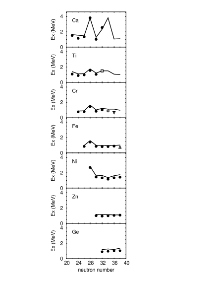
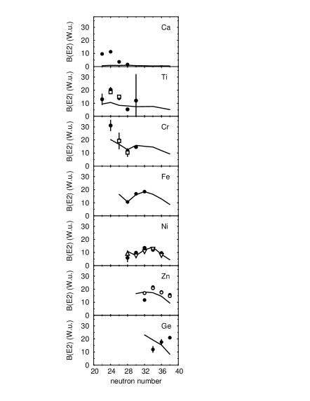
Figure 13: (Left) First 2⁺ energy levels as a function of the neutron number $N$. Experimental data are shown by filled circles nndc , square ti54 , open circle cr58 , triangle(down) cr60 , and triangle(up) hanna . Solid lines show results of shell-model calculations. The truncation order $t$ is 5 for ^56,58Fe, ⁶⁰Ni, ^60,62,64Zn, 6 for ^56,58,62Ni and 7 for ^52,54Fe. The other results are exact. (Right) The values of $B$(E2; $2^{+}_{1}\rightarrow 0^{+}_{1}$). Experimental data are shown by filled circles nndc , squares speidel , triangle (up) kraus , triangles (down) kenn , and open circles kenn65 .

III.6 Semi-magic nuclei

In this subsection, spectroscopic properties are studied in detail for several $N$ or $Z=28$ nuclei around ⁵⁶Ni. If we assume an inert closed core for ⁵⁶Ni, these semi-magic nuclei are described by a few valence nucleons of one kind, i.e., only proton holes or only neutron particles. Therefore, the low-lying level density is rather low and the effects of core-excitations are easy to interpret. In fact, it has been pointed out in Ref. nakada that, although the shell-model calculation in a truncated $t\leq 2$ subspace is quite successful for describing most of the low-lying stats in $N$=28-30 nuclei, it is impossible to reproduce those states which contain sizable broken-core components, such as the lowest excited states in ⁵⁵Co, excited states above the lowest $3/2^{-},5/2^{-},1/2^{-}$ triplets in ⁵⁷Ni, excited $0^{+}$ in ⁵⁴Fe and ⁵⁸Ni, etc. Similar difficulties can be seen also in Ref. rud-epj , where the shell-model calculations in a truncated space have been carried out with a different effective interaction. Note that the cause of this problem lies not only in the truncation of the model space but also in the effective interaction itself. It is well known that the KB3 interaction (and also its descendants) gives an excellent description for low-lying states of $A\leq 52$ nuclei, but KB3 fails around ⁵⁶Ni, even when the model space is sufficiently large for convergence. Thus it is interesting to investigate whether GXPF1 can properly describe these low-lying states which are sensitive to the core-excitation. We consider semi-magic nuclei with $Z$=25, 26, 27 and $N$=29, 30, 31.

III.6.1 ⁵³Mn

Figure 14 shows experimental and calculated energy levels of ⁵³Mn. Most of the theoretical energy levels are obtained in the $t=7$ subspace. The exact ($t$=13) results are also obtained in some cases. All experimental energy levels below 3 MeV excitation energy as well as the yrast states are shown with their theoretical counterparts and several additional states.

Figure 14: Experimental (right) and calculated (left) energy levels of ⁵³Mn. Experimental data are taken from nds-mn53 . The label “na” indicates that the spin-parity is not assigned experimentally. The calculated yrast states are connected with experimental counterparts (or their candidates) by dotted lines.

For the yrast states, the agreement between the theory and the experiment is quite good. Assuming an inert ⁵⁶Ni core, this nucleus is described by three neutron holes in the $f_{7/2}$ orbit. Under such an assumption, possible states are $J^{\pi}=3/2^{-}$, $5/2^{-}$, $7/2^{-}$, $9/2^{-}$, $11/2^{-}$ and $15/3^{-}$. In the calculated wave functions, the lowest $(f_{7/2})^{13}$ configuration is in fact dominant (46$\sim$60%) for the yrast states of these spin-parities. Therefore, the truncation of the model space by a small $t\sim$2 is reasonable for these states.

Other yrast states, $1/2^{-}$, $13/2^{-}$, $17/2^{-}$, $19/2^{-}$, $21/2^{-}$, $23/2^{-}$ and $25/2^{-}$ consist mainly of $\pi(f_{7/2})^{5}\nu(f_{7/2})^{7}(p_{3/2})^{1}$ and $\pi(f_{7/2})^{5}\nu(f_{7/2})^{7}(f_{5/2})^{1}$ configurations. These states are also well reproduced in the calculation, indicating that the effective single-particle gap above $N=28$ is reasonably reproduced in the present interaction.

In order to investigate the properties of the core in detail, it is important to consider non-yrast states which contain a large amount of multi-particle excitations from the $N=28$ core. Above $E_{x}\sim$ 2.2 MeV, the experimental level density increases significantly, which is well reproduced in the calculation. The largest difference between the experiment and the calculation is found for the $3/2^{-}_{2}$ state which lies at lower energy by 450 keV in the calculation, resulting in the inversion of $5/2^{-}_{2}$ and $3/2^{-}_{2}$. Nevertheless, one can find reasonable one-to-one correspondence between the experimental and theoretical energy levels.

Focusing on the neutron configuration, the main configuration of these non-yrast states is $\nu(f_{7/2})^{7}(r)^{1}$ [$r$ stands for ($p_{3/2}$,$f_{5/2}$,$p_{1/2}$)]. The typical probability for the neutron 1p-1h configuration is $\sim$60%. These states contain also multi-neutron excitations as 2p-2h ($\sim$25%) and 3p-3h ($\sim$7%). Therefore, taking into account the proton excitation, the $t\sim 4$ subspace is reasonable for describing these states.

Table 7: $B$(M1) and $B$(E2) for ⁵³Mn. The excitation energy ($E_{x}$) is shown in keV. Experimental data are taken from nds-mn53 .

initial	final	multi-	exp.	th.
$J^{\pi}(E_{x})$	$J^{\pi}(E_{x})$	pole	(W.u)	(W.u)
5/2-(378)	7/2-(0)	M1	$0.00254(23)$	$0.0060$
		E2	$14(3)$	$21.7$
3/2-(1290)	5/2-(378)	M1	$0.023(3)$	$0.0194$
		E2	$1.9(5)$	$0.6$
	7/2-(0)	E2	$13.4(11)$	$8.1$
11/2-(1441)	7/2-(0)	E2	$12.8(18)$	$9.4$
9/2-(1620)	5/2-(378)	E2	$3.7(6)$	$3.6$
	7/2-(0)	M1	$0.0012(3)$	$0.0002$
		E2	$7.0(9)$	$5.4$
5/2-(2274)	3/2-(1290)	M1	$0.0021(8)$	$0.0000$
		E2	$3.0(15)$	$0.0$
	5/2-(378)	M1	$0.0019(4)$	$0.0010$
		E2	$0.61(14)$	$1.6$
	7/2-(0)	M1	$0.0054(11)$	$0.0023$
		E2	$0.07(4)$	$0.02$
3/2-(2407)	3/2-(1290)	M1	$0.064(24)$	$0.0482$
		E2	$1.9(16)$	$0.3$
	5/2-(378)	M1	$>0.0038^{+22}_{-10}$	$0.0058$
		E2	$<0.43$	$1.0$
	7/2-(0)	E2	$2.0(9)$	$4.4$
13/2-(2563)	11/2-(1441)	M1	$0.00146(18)$	$0.0022$
		E2		$0.0$
1/2-(2671)	5/2-(378)	E2	$15(12)$	$2.7$
7/2-(2686)	5/2-(378)	M1	$0.004(4)$	$0.0014$
		E2		$0.1$
	7/2-(0)	M1	$0.010(9)$	$0.0100$
		E2	$2.4(22)$	$0.9$
15/2-(2693)	13/2-(2563)	M1	$0.21(4)$	$0.0183$
		E2		$4.7$
	11/2-(1441)	E2	$5.4(8)$	$3.3$
3/2-(2876)	5/2-(378)	M1	$2.5$E-$5(10)$	$0.0040$
		E2		$0.9$
	7/2-(0)	E2	$0.0008(3)$	$0.2$
9/2-(2947)	7/2-(0)	M1	$0.007(4)$	$0.0315$
		E2	$1.8(8)$	$3.9$
13/2-(3426)	11/2-(2698)	M1	$0.04(3)$	$0.0144$
		E2	$1.6$E+$2(12)$	$18.1$
15/2-(3439)	15/2-(2693)	M1	$0.23(4)$	$1.0585$
		E2	$2.$E+1$(5)$	$1.3$
19/2-(5614)	17/2-(4384)	M1	$>0.22$	$0.1183$
		E2		$16.1$
21/2-(6533)	17/2-(4384)	E2	$2.8(16)$	$7.0$
23/2-(7004)	21/2-(6533)	M1	$0.153(24)$	$0.1099$
		E2		$0.0$

However, even in this energy region of $E_{x}\sim 2.5$ MeV, there are several states in which the $N=28$ core is more severely broken. In $5/2^{-}_{2}$, $7/2^{-}_{2}$, $9/2^{-}_{2}$, the main neutron configuration is 2p-2h type ($\sim$60%), and also there are sizable broken-core components such as 3p-3h ($\sim$17%) and 4p-4h ($\sim$6%). Evidently, the $t=4$ subspace is no longer sufficient and at least $t=6$ is needed to describe these states properly. In fact, for example, the electric quadrupole moment for $5/2^{-}_{2}$ varies as $Q(5/2^{-}_{2})$=$-0.25$, $+0.32$, $+0.36$ and $+0.37$eb for $t$=4, 5, 6 and 13 (exact), respectively. The change of the sign in going from $t=4$ to $t=5$ is due to the crossing of $5/2^{-}_{2}$ and $5/2^{-}_{3}$. A similar crossing is found in the case of $7/2^{-}_{2}$. Although these neutron 2p-2h states are connected by relatively large (collective) M1 and E2 transition matrix elements as $B($E2$;7/2^{-}_{2}\rightarrow 5/2^{-}_{2})=34$ W.u. and $B($M1$;7/2^{-}_{2}\rightarrow 5/2^{-}_{2})=0.17$ W.u., it may be difficult to observe such transitions because of negligibly small gamma-ray energies in comparison to the transition to the yrast states.

In Table 7, calculated electro-magnetic transition probabilities are compared with experimental data. Reasonable agreement can be seen in most cases, including transitions between non-yrast states. Note that the theoretical $1/2^{-}_{2}$ is assigned to the experimental $1/2^{-}$ at 2671 keV so that the transition data can be consistently described.

III.6.2 ⁵⁴Fe

In Fig. 15, the energy levels of ⁵⁴Fe are compared with experimental data. All experimental energy levels below $E_{x}$=4 MeV and all yrast states are shown with their theoretical counterparts. Shell-model calculations have been carried out in the $t=7$ or larger subspace including the exact ($t$=14). One can see remarkable one-to-one correspondence between theory and experiment for most of these levels.

The yrast band $0^{+}$-$2^{+}$-$4^{+}$-$6^{+}$ shows a typical proton two hole spectrum in the $f_{7/2}$ orbit under the influence of a short range interaction. In fact the wave functions of these states are dominated by the $\pi(f_{7/2})^{6}\nu(f_{7/2})^{8}$ configuration (50-60%). On the other hand, the yrast $8^{+}$ and $10^{+}$ states consist of core-excited configurations. While the dominating configurations are still of neutron 1p-1h excitation type from the $N=28$ core (36% and 57% for $8^{+}$ and $10^{+}$ states, respectively), the wave functions can no longer be approximated by only one configuration. The energy gap between $6^{+}$ and $8^{+}$ reflects the softness of the ⁵⁶Ni core, which is determined by the effective interaction. It is shown in Ref. brazil that the energy gap is too large with the KB3 interaction. This is consistent with the fact that it also gives an energy for the yrast $2^{+}$ energy in ⁵⁶Ni which is too high compared with experiment.

Figure 15: Energy levels of ⁵⁴Fe. Experimental data are taken from nds-fe54 and rud-epj . Conventions are the same as in Fig. 14.

It was pointed out in Ref. semi that the FPD6 fpd6 interaction predicts the existence of deformed states at relatively low excitation energy ($\sim$3 MeV), which consist of neutron 2p-2h configurations. In the present calculation, the candidates of such states appear as $0^{+}_{2}$ and $2^{+}_{3}$. The neutron 2p-2h configuration is 35% and 26% in these states, respectively, which are the most dominant components in their wave functions. However, the deformation of these states is much smaller than the FPD6 prediction. The electric quadrupole moment for the “2p-2h” $2^{+}$ state is predicted to be $-0.30$eb semi by the variation after the angular momentum projection (VAP) method with the FPD6 interaction. On the other hand, in the present results, it is $Q(2^{+}_{3})=-0.09$ eb, and the E2 transition matrix element is $B(E2;2^{+}_{3}\rightarrow 0^{+}_{2})=11.3$ W.u., which is slightly larger than that of the yrast in-band transition. These values are inconsistent with the axially symmetric large prolate deformation. In the present results, two neutrons are excited mainly to the $p_{3/2}$ orbit, while it is $f_{5/2}$ in the results of the FPD6 interaction, reflecting the fact that the effective single particle energy for the $f_{5/2}$ orbit is too low for FPD6.

Table 8: $B$(M1) and $B$(E2) for ⁵⁴Fe. Experimental data are taken from nds-fe54 .

initial	final	multi-	exp.	th.
$J^{\pi}(E_{x})$	$J^{\pi}(E_{x})$	pole	(W.u)	(W.u)
2+(1408)	0+(0)	E2	$10.6(4)$	$10.7$
4+(2538)	2+(1408)	E2	$6.3(13)$	$5.5$
0+(2561)	2+(1408)	E2	$<16$	$3.8$
6+(2949)	4+(2538)	E2	$3.25(5)$	$3.3$
2+(2959)	2+(1408)	M1	$0.051(9)$	$0.0584$
		E2	$0.5(4)$	$0.2$
	0+(0)	E2	$2.2(4)$	$3.1$
2+(3166)	2+(1408)	M1	$0.0035(21)$	$0.0013$
		E2	$1.0(13)$	$1.7$
	0+(0)	E2	$0.74(19)$	$0.8$
4+(3295)	4+(2538)	M1	$<0.020$	$0.2727$
		E2	$<2.7$	$1.7$
	2+(1408)	E2	$<0.15$	$0.9$
3+(3345)	4+(2538)	M1	$<0.0086$	$0.0000$
		E2	$<0.022$	$0.9$
	2+(1408)	M1	$<0.00068$	$0.0004$
		E2	$<0.11$	$0.0$
4+(3833)	4+(3295)	M1	$0.011(12)$	$0.0312$
		E2	$8.E+1(9)$	$1.9$
	4+(2538)	M1		$0.0032$
		E2	$18(7)$	$0.0$
	2+(1408)	E2	$7.9(18)$	$8.6$
4+(4031)	4+(3295)	M1	$<0.033$	$0.0112$
		E2	$<1.3E2$	$0.1$
	4+(2538)	M1	$<0.0014$	$0.0514$
		E2	$<1.5$	$0.7$
4+(4048)	3+(3345)	M1	$0.15(7)$	$0.0764$
		E2	$32^{+28}_{-24}$	$16.3$
	2+(1408)	E2	$0.20(16)$	$0.3$
4+(4268)	4+(2538)	M1	$0.032(12)$	$0.0052$
		E2	$6(5)$	$4.8$
	2+(1408)	E2	$0.60(17)$	$0.5$
0+(4291)	2+(1408)	E2	$4.3(14)$	$4.3$
2+(4579)	2+(1408)	M1	$>0.067$	$0.0170$
		E2		$4.9$
	0+(0)	E2	$>0.99$	$0.7$
		M1	$0.0052(8)$	$0.0000$
8+(6381)	6+(2949)	E2	$0.86(22)$	$3.3$
10+(6527)	8+(6381)	E2	$1.69(4)$	$2.0$

In Table 8, the calculated electro-magnetic transition matrix elements are compared with experimental data. The E2 transition matrix elements in the ground-state band are reproduced fairly well in the present calculations, although the $8^{+}\rightarrow 6^{+}$ transition is overestimated. Such a deviation is commonly seen also in the results of KB3 and FPD6 interactions brazil . Other $B$(E2) values are reasonably reproduced except for several of the small ones. As for the $B$(M1) values, the agreement between theory and experiment is basically good. The exception is $4^{+}(3294)\rightarrow 4^{+}(2538)$ transition, which is significantly overestimated by more than one order of magnitude in the present calculation.

III.6.3 ⁵⁵Co

In Fig. 16, energy levels of ⁵⁵Co are shown. All experimental energy levels below $E_{x}$=4 MeV and all yrast states up to $J^{\pi}=23/2^{-}$ are compared with theoretical results. There is a state with unknown spin-parity at $E_{x}$=2.960 MeV, which can be interpreted tentatively as a $5/2^{-}$ state in the correspondence to the present calculation. The overall agreement between theory and experiment is quite good.

Figure 16: Energy levels of ⁵⁵Co. Experimental data are taken from nds-co55 and rud-epj . Conventions are the same as in Fig. 14.

If we assume an inert ⁵⁶Ni core, this nucleus is described as one neutron hole in the $f_{7/2}$ orbit, corresponding to only one $7/2^{-}$ state. In the calculated ground-state wave function, the probability of this 0p-1h configuration relative to the ⁵⁶Ni core is only 65%, and there are sizable ($\sim$20%) 2p-3h configurations. All excited states consist of core-broken configurations even in the lowest order of the approximation. Therefore the property of the core is expected to manifest clearly in the yrast spectrum.

The yrast states up to $J^{\pi}=17/2^{-}$ except for the ground state are described mainly by 1p-2h configurations (30$\sim$56%). Thus the truncated subspace with small $t\sim 2$ is expected to be reasonable. In fact the truncated $t=2$ subspace was used in the shell-model calculations of Ref. rud-epj , where $13/2^{-}$ and higher spin states are described reasonably well. However, the excitation energies of lower spin states $9/2^{-}$ and $11/2^{-}$ are predicted to be too high by $\sim$1 MeV, and the results of $5/2^{-}$, $3/2^{-}$ and $1/2^{-}$ are not shown in Ref. rud-epj .

A part of such a difficulty may be attributed to the severe truncation. In the present $t=7$ results, the position of both these higher ($J^{\pi}\geq 13/2^{-}$) and lower spin states are successfully described. In the lower spin states, there are sizable 3p-4h ($\sim$21%) and 4p-5h ($\sim$9%) components, including both proton and neutron excitations almost equally. On the other hand, the higher spin states $13/2^{-}$, $15/2^{-}$ and $17/2^{-}$ are described mainly by neutron excitations only, and the probabilities of 3p-4h and 4p-5h components are much smaller ($\sim$16% and 6%, respectively). When the GXPF1 interaction is used in the $t=2$ subspace, the excitation energies of lower spin states becomes too large by about 0.4 MeV, while those of higher spin states are almost unchanged.

For constructing higher spin states, it is necessary to excite one more nucleon from the $f_{7/2}$ orbit. In fact the most dominant component in the wave function of these states is the 2p-3h type ($\sim$45%). A large gap ($\sim$2 MeV) between $17/2^{-}$ and $19/2^{-}$ reflects this core-excitation. Note that, although it is possible to construct a $19/2^{-}$ state within the 1p-2h configuration space, this component is only 9% in the $19/2^{-}_{1}$ state, similarly to the result in Ref. rud-epj . The present calculations successfully reproduce both 1p-2h and 2p-3h excitations.

Table 9: $B$(M1) and $B$(E2) for ⁵⁵Co. Experimental data are taken from nds-co55 .

initial	final	multi-	exp.	th.
$J^{\pi}(E_{x})$	$J^{\pi}(E_{x})$	pole	(W.u)	(W.u)
3/2-(2166)	7/2-(0)	E2	$9.8(8)$	$8.1$
3/2-(2566)	7/2-(0)	E2	$1.05(25)$	$1.3$
1/2-(2939)	3/2-(2566)	M1	$0.9^{+7}_{-3}$	$0.1130$
		E2		$25.9$
	3/2-(2166)	M1	$0.27^{+20}_{-8}$	$0.1371$
		E2	$34^{+48}_{-28}$	$0.2$
5/2-(3303)	7/2-(0)	M1	$0.0089(20)$	$0.0132$
		E2	$0.15(6)$	$0.03$
1/2-(3323)	3/2-(2566)	M1	$0.47(12)$	$0.3100$
		E2		$7.0$
	3/2-(2166)	M1	$0.17(4)$	$0.2514$
		E2		$9.7$
5/2-(3725)	3/2-(2566)	M1	$0.092(21)$	$0.0398$
		E2	$<0.4$	$0.3$
	7/2-(0)	M1	$0.0055(11)$	$0.0263$
		E2	$0.03(3)$	$0.00$
1/2-(4164)	3/2-(2566)	M1	$0.157(20)$	$0.2194$
		E2	$9(3)$	$3.5$

The structure of non-yrast states is more complicated. Since the present interest is the low-lying core-excited states, we can focus on $1/2^{-}_{2}$, $3/2^{-}_{3}$, $7/2^{-}_{3}$ and $5/2^{-}_{3}$. These states are all below $E_{x}$=4 MeV and contain more than 45% neutron 2p-2h components. A similar character can also be seen in $3/2^{-}_{2}$, although the probability of the neutron 2p-2h component is slightly smaller (37%). These states are connected by relatively large E2 transition matrix elements such as $B$(E2; $7/2^{-}_{3}\rightarrow 3/2^{-}_{2}$)=11 W.u. and $B$(E2; $5/2^{-}_{3}\rightarrow 1/2^{-}_{2}$)=18 W.u. It will be a good test if it is possible to observe such transitions.

The calculated $3/2^{-}_{4}$ has isospin $T=3/2$ and is the isobaric analog state of the ⁵⁵Fe ground state. The correct position of this state, as seen in comparison to experiment in Fig. 16, implies the proper isospin structure of the present interaction.

In Table 9, electro-magnetic transition matrix elements are shown for ⁵⁵Co. We can find reasonable agreement between theory and experiment. In general, the deviations are large where the experimental errors are also large.

III.6.4 ⁵⁶Ni

In Fig. 17, calculated energy levels of ⁵⁶Ni are compared with experimental data. All calculated states up to $E_{x}$=6 MeV as well as the yrast states are shown. The shell-model results were obtained in the $t=7$ subspace. The agreement between the experiment and the calculation is basically good especially for even spin yrast states. However, the yrast $3^{+}$ and $5^{+}$ states are not found in the experimental data, while no candidate for the experimental $(2^{+})$, $(4^{+})$ and $(6^{+})$ can be seen in the calculation at least around $E_{x}\sim$6 MeV. More precise experimental information is needed to discuss such discrepancies. Similar results are shown in Fig. 2 of Ref. upf for even spin states, which were obtained by the MCSM calculations, taking typically 13 bases per one eigenstate. We thus confirm the reliability of the MCSM results for non-yrast states.

Figure 17: Energy levels of ⁵⁶Ni. Experimental data are taken from nds-ni56 and rud-epj . Conventions are the same as in Fig. 14.

For the yrast states, the ground state consists mainly of the $(f_{7/2})^{16}$ closed-shell configuration (68%). The excited states $2^{+}$, $3^{+}$, $4^{+}$, $5^{+}$ and $6^{+}$ are of the 1p-1h character (42$\sim$50%) relative to the closed-shell configuration, and the excitation energy of $2^{+}_{1}$ reflects the shell gap at $N$ or $Z=28$. The 2p-2h configurations are dominant in $1^{+}$, $7^{+}$, $8^{+}$, $9^{+}$ and $10^{+}$ states (35$\sim$51%). One can find again an energy gap between these 1p-1h and 2p-2h groups. The 3p-3h dominant states appear above $E_{x}\sim$10 MeV. In the same way, most of the non-yrast excited states shown in the figure can be classified as either 1p-1h ($3^{+}_{2}$, $5^{+}_{2}$, $\cdots$) or 2p-2h ($2^{+}_{2}$, $6^{+}_{2}$, $\cdots$) dominant states. These $n$p-$n$h states contain typically 20% of $(n+2)$p-$(n+2)$h configurations. Therefore, the 4p-4h configuration space is essential (but not enough) to describe these states.

As has already been discussed in Ref. upf , GXPF1 predicts the deformed 4p-4h band rudolph as 0${}^{+}_{3}$, $2^{+}_{2}$, $\cdots$. In the present results, $0^{+}_{3}$ consists mainly of 4p-4h (48%), 5p-5h (23%) and 6p-6h (12%) configurations. The structure of $2^{+}_{2}$ is quite similar. Special care should be taken concerning the convergence of the calculation for such a deformed 4p-4h band, since the present truncation scheme is obviously not suitable for describing strongly deformed states, as discussed in Ref. ni56super for the case of the FPD6 interaction. Figure 18 shows the calculated energies and quadrupole moments of the lowest two $2^{+}$ states as a function of the truncation order $t$. It can be seen that the 4p-4h state $2^{+}_{2}$ is not completely converged even in the $t=7$ subspace, which corresponds to the $M$-scheme dimension of 89285264. In the same figure, the MCSM results are also shown, where 25 bases were searched for each eigenstate. The MCSM energy of the yrast 2⁺ state is almost the same as that of the $t=7$ calculation, which shows reasonable convergence. On the other hand, for $2^{+}_{2}$ states, the MCSM energy is lower than the $t=7$ result by about 0.2 MeV, and should be more accurate. The electric quadrupole moment is $Q(2^{+}_{2})=-41.2$efm² in the MCSM calculation, while it is $-33.6$ in the present $t=7$ result. Similar results are obtained for the 4p-4h 0${}^{+}_{3}$ state. The $M$-scheme dimension of $t=8$ subspace reaches to 255478309, which is beyond our computational limitations. For the description of such deformed states where a lot of mixing among various spherical configurations occurs, the MCSM calculation is more efficient and suitable, because certain basis states can be sampled from and around local minima.

Figure 18: Convergence of the calculated energies (lower panel) and quadrupole moments (upper panel) as functions of the truncation order $t$ for the lowest two 2⁺ states of ⁵⁶Ni. Horizontal lines show the corresponding MCSM results.

In the present results, we can find several $T=1$ states such as $0^{+}_{4}$, $2^{+}_{4}$ and $4^{+}_{5}$. These states are interpreted as the isobaric analog states of ⁵⁶Co. The excited $0^{+}$ with $T=1$ is in fact found experimentally at excitation energy of 7.904 MeV, which is consistent with the present result.

Experimental data for the electro-magnetic transitions are rather limited. We can only compare with the few transition strengths shown in Table 10.

Table 10: $B$(M1) and $B$(E2) for ⁵⁶Ni. Experimental data are taken from nds-ni56 and kraus .

initial	final	multi-	exp.	th.
$J^{\pi}(E_{x})$	$J^{\pi}(E_{x})$	pole	(W.u)	(W.u)
2+(2701)	0+(0)	E2	$9.4(1.9)$	$11.1$
4+(3924)	2+(2701)	E2	$<24$	$8.4$
6+(5317)	4+(3924)	E2		$5.4$
2+(5351)	2+(2701)	E2		$4.1$
	0+(0)	E2		$0.1$
8+(7956)	6+(5317)	E2		$0.1$
10+(9419)	8+(7956)	E2		$0.1$

III.6.5 ⁵⁷Ni

Energy levels of ⁵⁷Ni are shown in Fig. 19. All experimental yrast levels as well as non-yrast states up to 4 MeV excitation energy are compared with the theoretical predictions. The shell-model calculations were carried out in the $t=6$ subspace. The agreement between experiment and theory is basically good up to high spin states $23/2^{-}$, although there are several inversion of the order of two closely lying states, such as $7/2^{-}_{1}$ and $5/2^{-}_{2}$.

Figure 19: Energy levels of ⁵⁷Ni. Experimental data are taken from nds-ni57 and rud-epj . Conventions are the same as in Fig. 14.

Comparing the present results with the previous MCSM ones in Ref. upf , we can again confirm the reliability of the MCSM calculations for non-yrast states as well as the yrast states of odd-mass nuclei. The root mean square difference of the excitation energies between the present and the previous MCSM results is 154 keV for 19 states shown in Fig. 2 of Ref. upf .

If we assume an inert ⁵⁶Ni core, ⁵⁷Ni is described by only one neutron. Then, three states $3/2^{-}$, $5/2^{-}$ and $1/2^{-}$ are possible, corresponding to the occupation of $p_{3/2}$, $f_{5/2}$, and $p_{1/2}$ orbits by one neutron. According to the present calculations, the lowest three states show such a “single particle” character, although there is a sizable mixing of the broken-core configurations. In fact, the pure “single particle” configurations are 62, 58 and 46%, respectively, in the calculated wave functions. Since the closed core configuration in the ground state of ⁵⁶Ni is 69% upf , the core is further broken in the ground state of ⁵⁷Ni, as can also be seen in Fig. 9.

The bare single particle energy of the $f_{5/2}$ orbit relative to the $p_{3/2}$ orbit is found to be 4.3 MeV in GXPF1. (see Table 1). The effective single particle energy (ESPE) kb3 ; mcsm-n20 of the $f_{5/2}$ orbit relative to the $p_{3/2}$ orbit decreases rapidly as the proton $f_{7/2}$ orbit is occupied, and reaches 1.1 MeV at ⁵⁷Ni. The mechanism for this behavior of the $f_{5/2}$ orbit is explained by the strong attraction between the protons in the $f_{7/2}$ orbit and neutrons in the $f_{5/2}$ orbit due to a strong $j_{>}$ - $j_{<}$ coupling term in the nuclear force, as discussed in Ref. magic . Thus the proper contribution of the two-body interaction, especially the monopole part, is needed to reproduce the experimental order of the lowest three states in ⁵⁷Ni. The FPD6 interaction is too strong in this respect, giving an ESPE for the $f_{5/2}$ orbit which is too low for the Ni isotopes. Note that, the ESPE’s of the $f_{5/2}$ and the $p_{1/2}$ orbit are still too large by 0.3 and 0.9 MeV, respectively, in comparison to the experimental excitation energies of $5/2^{-}$ and $1/2^{-}$ states, since they are defined in terms of a closed-shell structure for ⁵⁶Ni. Further energy gain by the mixing of the broken-core components is needed for the better reproduction of the experimental data.

There is an energy gap ($\sim$ 1.3 MeV) above the lowest three states, which corresponds to the 2p-1h core-excitation. The doublets $5/2^{-}_{2}$ and $7/2^{-}_{1}$ consist of two dominant configurations, $\pi(f_{7/2})^{7}(p_{3/2})^{1}\nu(f_{f7/2})^{8}(p_{3/2})^{1}$ and $\pi(f_{7/2})^{8}\nu(f_{f7/2})^{7}(p_{3/2})^{2}$, sharing almost equal probabilities ($\sim$20%). Above these doublets, most of the states up to $E_{x}\sim$5 MeV are also of the 2p-1h nature, although one can no longer find single dominant configuration which exhausts more than 20% probability. In this 2p-1h regime, as exceptional cases, the $3/2^{-}_{3}$ and $1/2^{-}_{2}$ states are comprised mainly of higher configurations: the 3p-2h configuration takes the largest weight (25 and 29%, respectively) and even the 5p-4h configuration can be seen with a non-negligible probability ($\sim$5%). In the yrast $15/2^{-}$ and most of the higher spin states, the 3p-2h configuration becomes dominant, carrying more than 40% probability. We have not identified 4p-3h or more significantly core-broken states such as those of the deformed 4p-4h band in the ⁵⁶Ni in the present results for ⁵⁷Ni.

Electro-magnetic transition strengths are shown in Table 11. Because of the large ambiguities in the experimental data, it is difficult to draw a definite conclusion. Most of the calculated M1 transitions are consistent with the experimental data. A notable deviation is found in the $B$(M1; $5/2^{-}_{1}\rightarrow 3/2^{-}_{1}$), where the calculated value is too small by a factor of 8. As for the E2 transitions, it can be seen that the calculated $B$(E2) values are in general smaller than the experimental data. The exception is the transition from $5/2^{-}$(2443). However, no experimental error is indicated in the data and only the upper bound is given for the associated M1 transition. The calculated $B$(E2) value does not contradict with the experimental lifetime data.

Table 11: $B$(M1) and $B$(E2) for ⁵⁷Ni. Experimental data are taken from nds-ni57 .

initial	final	multi-	exp.	th.
$J^{\pi}(E_{x})$	$J^{\pi}(E_{x})$	pole	(W.u)	(W.u)
5/2-(769)	3/2-(0)	M1	$0.0144(18)$	$0.0018$
		E2	$2.5(6)$	$1.4$
1/2-(1113)	3/2-(0)	M1	$\leq\,0.19$	$0.1317$
		E2	$\leq\,3.0E+2$	$7.3$
5/2-(2443)	3/2-(0)	M1	$<0.024$	$0.0003$
		E2	$0.049$	$10.7$
7/2-(2577)	3/2-(0)	E2	$7.7(11)$	$7.4$
3/2-(3007)	3/2-(0)	M1	$<0.13$	$0.0229$
		E2	$<27$	$7.2$
11/2-(3866)	7/2-(2577)	E2	$42^{+24}_{-10}$	$6.8$
15/2-(5321)	11/2-(3866)	E2	$10^{+4}_{-2}$	$4.5$

III.6.6 ⁵⁸Ni

Figure 20 shows calculated and experimental energy levels of ⁵⁸Ni. The yrast states up to 10 MeV excitation energy, non-yrast states below $E_{x}$=4 MeV, and several additional states are shown with their theoretical counterparts. The agreement between the experiment and the calculation is satisfactory. The calculations were carried out in the $t$=6 truncated subspace. The results are basically consistent with our previous MCSM calculations in Ref. upf , although the latter spectrum was slightly expanded for higher spin states due to the small number of basis states ($\sim$13 per one eigenstate).

Figure 20: Energy levels of ⁵⁸Ni. Experimental data are taken from nds-ni58 . Conventions are the same as in Fig. 14.

In the calculated ground-state wave function, the total probability of the closed core configurations $\pi(f_{7/2})^{8}\nu(f_{7/2})^{8}(r)^{2}$ is only 57%, which is smaller than those in ^56,57Ni. As shown in Fig. 9, this quantity decreases further for larger $N$ and takes a minimum value at $N=34$ (52%). Thus the ⁵⁶Ni core is soft in Ni isotopes. Nevertheless, for understanding the basic structure, it is still useful to assume an inert ⁵⁶Ni core and to consider two neutrons in the $p_{3/2}$, $f_{5/2}$ and $p_{1/2}$ orbits. Then, the allowed maximum spin is $J=4$, and core-excitation is needed to generate higher spin states. In the calculated wave function, the leading configuration is $\nu(p_{3/2})^{2}$ for $0^{+}_{1}$ and $2^{+}_{1}$ (37% and 30%, respectively), and $\nu(p_{3/2})^{1}(f_{5/2})^{1}$ for $1^{+}_{1}$ and $3^{+}_{1}$ (42% and 52%, respectively). There is a large energy gap ($\sim$ 2 MeV) in the yrast spectrum between $4^{+}_{1}$ and $5^{+}_{1}$, reflecting the core-excitation. One-proton core-excitation dominates the wave functions up to $J=9$, although there is no single configuration which exhausts more than 20% weight in the calculated wave functions. For $J=10$ and higher spin yrast states one-proton one-neutron core-excitation becomes the most important mode. Consistently, there is another energy gap ($\sim$ 1.6 MeV) above $9^{+}_{1}$ in both calculated and experimental energy spectra.

The closed-core configurations also play a major role in many non-yrast states. Among the non-yrast states below $E_{x}\sim$ 4 MeV, the 3p-1h configurations associated with the one-proton core-excitation become dominant in $2^{+}_{3}$, $4^{+}_{2}$ and $3^{+}_{2}$. Since the level density increases significantly above $E_{x}\sim$ 4 MeV, it is difficult to make a simple interpretation for the properties of the core-excitations in higher states.

As discussed in Ref. upf , the core-excitation of two-protons is dominant in the wave function of $0^{+}_{3}$. In the present calculation, we found that $2^{+}_{6}$ shows a similar 4p-2h character. The probability of such a 4p-2h configuration $\pi(f_{7/2})^{6}(r)^{2}\nu(f_{7/2})^{8}(r)^{2}$ is 46 and 41% for $0^{+}_{3}$ and $2^{+}_{6}$, respectively. The calculated quadrupole moment is $Q(2^{+}_{6})=-0.30$ eb, and $B$(E2; $2^{+}_{6}\rightarrow 0^{+}_{3}$)=18 W.u. These values are consistent with those of the rotational model, corresponding to the $K=0$ band on top of the axially symmetric prolate rotor with an intrinsic quadrupole moment $Q_{0}$=110 eb. The deformation of the present 4p-2h band appears to be slightly smaller than the 4p-4h band in ⁵⁶Ni upf , which is consistent with $Q_{0}$=140 eb obtained by using the same effective charges.

Table 12: $B$(M1) and $B$(E2) for ⁵⁸Ni. Experimental data are taken from nds-ni58 .

initial	final	multi-	exp.	th.
$J^{\pi}(E_{x})$	$J^{\pi}(E_{x})$	pole	(W.u)	(W.u)
2+(1454)	0+(0)	E2	$9.8(5)$	$7.7$
4+(2459)	2+(1454)	E2	$<43$	$4.1$
2+(2775)	2+(1454)	M1	$0.011(4)$	$0.1103$
		E2	$15(5)$	$1.2$
	0+(0)	E2	$0.029(10)$	$2.8$
0+(2942)	1+(2902)	M1	$0.084(6)$	$0.0068$
	2+(2775)	E2	$14.9(18)$	$12.4$
	2+(1454)	E2	$0.00029(4)$	$0.63$
2+(3038)	2+(2775)	M1	$0.23(6)$	$0.0275$
		E2	$6^{+20}_{-6}$	$1.0$
	2+(1454)	M1	$0.060(12)$	$0.0190$
		E2	$2.0(7)$	$15.0$
2+(3263)	2+(1454)	M1	$0.028(11)$	$0.0004$
		E2	$8(7)$	$0.01$
3+(3420)	4+(2459)	M1	$0.09(8)$	$0.1101$
		E2	$0.07^{+23}_{-7}$	$0.11$
0+(3531)	2+(1454)	E2	$5.5$	$3.5$
4+(3620)	4+(2459)	M1	$0.07^{+7}_{-4}$	$0.0002$
		E2	$44^{+60}_{-36}$	$1.3$
	2+(1454)	E2	$1.4^{+12}_{-6}$	$6.7$
3+(3774)	3+(3420)	M1	$0.33(17)$	$0.0169$
		E2	$1.$E$+1^{+11}_{-1}$	$0.1$
	4+(2459)	M1	$0.019(10)$	$0.0001$
		E2	$0.8^{+12}_{-8}$	$0.4$
2+(3898)	2+(1454)	M1	$0.042^{+25}_{-11}$	$0.0410$
	0+(0)	E2	$0.42^{+25}_{-11}$	$0.81$
2+(4108)	2+(2775)	M1	$0.0051(20)$	$0.0089$
	2+(1454)	M1	$0.0032(8)$	$0.0003$
		E2	$0.30(10)$	$0.29$
	0+(0)	E2	$0.15(4)$	$0.08$

In Table 12, calculated transition strengths are compared with experimental data. In general, the calculated M1 matrix elements are too small. The exception is $B$(M1; $2^{+}_{2}\rightarrow 2^{+}_{1}$), which is too large by one order of magnitude. As for the E2 matrix elements, the calculated values are almost consistent with experimental data in the case of $\Delta J=2$ transitions, i.e., no mixing of M1 transitions. One notable exception is $B$(E2; $0^{+}_{2}\rightarrow 2^{+}_{1}$), which is too large by more than 3 orders of magnitude, but this is an extremely weak transition.

III.6.7 ⁵⁹Ni

Energy levels of ⁵⁹Ni are shown in Fig. 21. All experimental data for yrast states as well as non-yrast states below 3 MeV excitation energy are compared with the shell-model results obtained in the $t$=6 subspace. It is found that the theoretical results agree quite well with the experimental data. The results of the lowest triplet $3/2^{-}$, $5/2^{-}$ and $1/2^{-}$ have already been reported in Ref. upf . The present calculation has confirmed the validity of GXPF1 interaction also for higher excited states.

Assuming an inert ⁵⁶Ni core, this nucleus is described by three valence neutrons in the upper three orbits $p_{3/2}$, $f_{5/2}$ and $p_{1/2}$. Therefore various states are possible without any core-excitation. In fact such closed-shell (3p-0h) configurations carry the maximum weight (31%$\sim$56%) in most of the calculated low-lying states below $E_{x}$= 3 MeV. There are three exceptions, $7/2^{-}_{2}$, $7/2^{-}_{3}$ and $11/2^{-}_{1}$, where 4p-1h configurations take the largest weight. Such 4p-1h configurations also dominate the wave functions of higher-lying excited states shown in the same figure. The 5p-2h configurations appears to be the leading configurations in the yrast $19/2^{-}$ and $21/2^{-}$ states.

Like other nuclei, we would like to identify states with large components of 5p-2h or higher configurations at $E_{x}<\sim 3$ MeV. This energy boundary is set because the level density increases very fast above it in ⁵⁹Ni. However, as seen from the above discussions, there are no such candidate states theoretically or experimentally. Therefore, the study of 5p-2h and higher states with lower angular momenta is not possible in ⁵⁹Ni. Thus, the discussion of the multi-particle multi-hole states which is one of the main elements in our assessment of the effective interaction is confined mainly to a few nuclei around ⁵⁶Ni.

Figure 21: Energy levels of ⁵⁹Ni. Experimental data are taken from nds-ni59 . Conventions are the same as in Fig. 14.

Table 13 shows the measured and calculated $B$(E2) and $B$(M1). Even below $E_{x}$=2 MeV, there are several uncertain levels in the experimental data at 1695 keV (no spin assignment), 1739 keV (assigned to ($9/2^{-}$)), and 1746 keV (assigned to $5/2^{-}$,$7/2^{-}$). In the present calculations, we have tentatively assigned no theoretical states to these three uncertain states, since no probable candidates appear around $E_{x}\sim$ 2 MeV. More experimental information is needed for a detailed comparison between theory and experiment.

In general, the order of magnitude is well reproduced for most transitions. More specifically, the calculated M1 transition matrix elements are small in comparison to the experimental data in many cases, except for $1/2^{-}_{1}\rightarrow 3/2^{-}_{1}$ transition. The calculated E2 matrix elements are also smaller than the experimental data. However, one can clearly see the correlation between the calculated values and the corresponding experimental data. The agreement could be improved if we introduced larger effective charges.

Table 13: $B$(M1) and $B$(E2) for ⁵⁹Ni. Experimental data are taken from nds-ni59 .

initial	final	multi-	exp.	th.
$J^{\pi}(E_{x})$	$J^{\pi}(E_{x})$	pole	(W.u)	(W.u)
5/2-(339)	3/2-(0)	M1	$0.0083(10)$	$0.0031$
		E2		$0.26$
1/2-(465)	3/2-(0)	M1	$0.011(2)$	$0.0705$
		E2		$1.7$
3/2-(878)	3/2-(0)	M1	$0.068(13)$	$0.0327$
		E2	$1.1(9)$	$7.0$
5/2-(1189)	3/2-(0)	M1	$0.043(9)$	$0.0058$
		E2	$11(5)$	$10.1$
1/2-(1301)	1/2-(465)	M1	$0.036(8)$	$0.0016$
	5/2-(339)	E2	$1.2(4)$	$0.4$
7/2-(1338)	5/2-(339)	M1	$0.0008(3)$	$0.0002$
		E2	$30(7)$	$10.7$
	3/2-(0)	E2	$2.9(7)$	$0.8$
5/2-(1680)	1/2-(465)	E2	$1.41(23)$	$0.20$
	3/2-(0)	M1	$0.0009(7)$	$0.0095$
		E2	$1.6(5)$	$1.1$
9/2-(1768)	7/2-(1338)	M1	$0.042(11)$	$0.0210$
		E2	$4^{+5}_{-3}$	$1.8$
	5/2-(339)	E2	$11(3)$	$3.3$
7/2-(1948)	5/2-(1189)	M1	$0.042(9)$	$0.0368$
		E2	$10(10)$	$0.9$
	3/2-(878)	E2	$3.6(10)$	$2.7$
	3/2-(0)	E2	$5.3(10)$	$7.2$
11/2-(2705)	9/2-(1768)	M1	$0.0040(13)$	$0.0005$
		E2	$8(3)$	$1.7$
	7/2-(1338)	E2	$22(6)$	$4.5$

III.7 $N$=$Z$ odd-odd nuclei

In the $pf$ shell, $N=Z$ odd-odd nuclei have been of special interest, where the lowest isospin $T$=0 and $T=1$ states are almost degenerate near the ground state. In most cases $T=1$, $J=0$ is the ground state. The only known exception is ⁵⁸Cu, in which the ground state is $T=0$, $J=1$. This reflects a detailed interplay of $T=0$ and $T=1$ interactions, and it is important to evaluate the effective interaction from this viewpoint.

III.7.1 ⁵⁴Co

In Fig. 22, calculated energy levels of ⁵⁴Co are compared with experimental data. The spin-parity has not been assigned to most of the states above $E_{x}=$ 3 MeV, and there are several uncertain levels among low-lying states. It can be seen that the present shell-model calculations in the $t=6$ subspace give a reasonable description, although there are several small deviations such as the interchange of the order of $2^{+}_{1}$ and $3^{+}_{1}$. The calculated $0^{+}_{1,2}$, $2^{+}_{1}$, $4^{+}_{3,4}$ and $6^{+}_{2}$ are $T=1$, corresponding to the isobaric analog states of ⁵⁴Fe (see Fig. 15), while other calculated states shown in the figure are $T=0$.

In the calculated wave functions of the yrast odd-spin states $1^{+}_{1}$, $3^{+}_{1}$, $5^{+}_{1}$ and $7^{+}_{1}$, the lowest $\pi(f_{7/2})^{7}\nu(f_{7/2})^{7}$ configuration is dominant (59, 58, 39 and 62%, respectively), but core-excited components are not small. Such lowest 0p-2h configurations relative to ⁵⁶Ni core are also dominant in even-spin $0^{+}_{1}$, $2^{+}_{1}$, $4^{+}_{3}$, and $6^{+}_{2}$, which are all $T=1$.

In the shell-model calculations co54 using the Surface Delta interaction in the ($f_{7/2}$, $p_{3/2}$) space with a restriction that the $p_{3/2}$ orbit can be occupied by one proton and one neutron, the $4^{+}$ and $6^{+}$ states of $T=1$ appear as yrast states. On the other hand, $4^{+}_{1,2}$ are isospin $T=0$ in the present calculation. If the calculated $4^{+}_{1}$ is assigned to the experimental state $(3^{+},4^{+})$ at 2083 keV, the agreement between theory and experiment is good. This state consists mainly of the 1p-3h configurations (50%). A similar structure can be seen for $6^{+}_{1}$, $5^{+}_{2}$, $7^{+}_{2}$, and $8^{+}_{1,2}$, where one nucleon is excited across the shell gap mainly to the $p_{3/2}$ orbit. The structure of $4^{+}_{2}$ is similarly of the 1p-3h type, although the excitation to the $f_{5/2}$ orbit is dominant. Such an excitation is also large in $8^{+}_{2}$.

One can find a $1^{+}_{2}$ state in the calculated spectra at a reasonable excitation energy, which does not appear in the shell-model results of Ref. co54 . The most important configuration in this state is $\pi(f_{7/2})^{6}(p_{3/2})^{1}\nu(f_{7/2})^{6}(p_{3/2})^{1}$, but its probability is only 15%. Such 2p-4h configurations are 44% in total, and there are other sizable core-excited components such as the 3p-5h (32%) and 4p-6h (17%) types. Similar core-excitations also appear in $2^{+}_{2}$, $3^{+}_{2}$ and $0^{+}_{2}$ ($T=1$).

Figure 22: Energy levels of ⁵⁴Co. Experimental data are taken from nds-co54 and rud-epj . Conventions are the same as in Fig. 14.

The calculated M1 and E2 transition strengths are listed in Table 14. Since no experimental value is available, the present results are compared with those of the shell-model calculation in Ref. co54 . Both results agree within a factor of about 2 for transitions between the states which consist mainly of the 0p-2h configurations. The strong isovector M1 transitions predicted based on the “quasideuteron” picture qdc are found also in the present large scale calculations. Note that the effective spin g-factors $g_{s}^{\rm eff}=0.7g_{s}^{\rm free}$ were used in Ref. co54 . If we adopt the same g-factors in the present calculations, the $B$(M1) values are significantly reduced, for example, $B$(M1; $1^{+}_{1}\rightarrow 0^{+}_{1}$) becomes 1.25 W.u. Thus the configuration mixing strongly affects the $B$(M1) value.

Several results related to the $1^{+}$ (1614), $3^{+}$ (2174) and $4^{+}$ (2852) states are very different between two calculations, because the structure of the corresponding states are different as mentioned above.

Table 14: $B$(M1) and $B$(E2) for ⁵⁴Co.

initial	final	multi-	Th-2. of Ref. co54	th.
$J^{\pi}(E_{x})$	$J^{\pi}(E_{x})$	pole	(W.u)	(W.u)
1+(937)	0+(0)	M1	$2.13$	$1.90$
2+(1446)	1+(937)	M1	$2.33$	$2.36$
		E2	$0.033$	$0.078$
	0+(0)	E2	$10.6$	$7.7$
3+(1822)	2+(1446)	M1	$2.36$	$1.92$
		E2	$0.091$	$0.155$
	1+(937)	E2	$10.6$	$4.2$
3+(2174)	2+(1446)	M1	$0.016$	$0.0055$
		E2	$0.0012$	$0.0000$
	1+(1614)	E2	$1.1$	$16.0$
	1+(937)	E2	$0.29$	$0.06$
4+(2652)	3+(1822)	M1	$2.00$	$1.95$
		E2	$0.18$	$0.39$
	2+(1446)	E2	$7.8$	$3.6$
	5+(1887)	M1	$2.13$	$1.07$
		E2	$0.21$	$0.29$
4+(2852)	3+(1822)	M1	$0.002$	$0.0000$
		E2	$0.12$	$0.02$
	5+(1887)	M1	$0.004$	$0.0000$
		E2	$7.1$	$0.03$

III.7.2 ⁵⁸Cu

In Fig. 23, the calculated energy levels of ⁵⁸Cu are compared with experimental data. All experimental states up to 2.2 MeV as well as the yrast states are shown. The shell-model calculations have been carried out in the $t=6$ truncated subspace. The agreement between theory and experiment is satisfactory. In the calculated spectrum, $0^{+}_{1}$, $2^{+}_{2}$, $4^{+}_{3}$ and $0^{+}_{2}$ are isospin $T=1$. The $T_{z}=1$ members of the multiplets can in fact be seen in the calculated spectrum of ⁵⁸Ni (see Fig. 20). The $T=0$ ground state $1^{+}_{1}$ is successfully reproduced.

Figure 23: Energy levels of ⁵⁸Cu. Experimental data are taken from nds-cu58 and rud-epj . Conventions are the same as in Fig. 14.

Assuming an inert ⁵⁶Ni core, one proton and one neutron are valence particles in the $p_{3/2}$, $f_{5/2}$ and $p_{1/2}$ orbits. Therefore $J\leq 5$ states are possible. In the calculated wave functions, the yrast states up to $5^{+}$ are in fact dominated by such closed core configurations with probabilities of $44\sim 63\%$. The $6^{+}_{1}$ state consists mainly of 3p-1h configurations (45%). The 4p-2h configurations are dominant in $7^{+}_{1}$, $8^{+}_{1}$, $9^{+}_{1}$ and $10^{+}_{1}$ (41$\sim$59%), and the 5p-3h configurations become the major components in $11^{+}_{1}$ and $12^{+}_{1}$ ($\sim$40%). Thus it is natural that the $t=2$ shell-model results in Ref. rud-epj show apparent discrepancies from experiment for $11^{+}$ and $12^{+}$.

In the present calculation, all states with $J\leq 10$ are dominated by either 3p-1h or 4p-2h configurations. Therefore, shell-model calculations even in the severely truncated ($t\sim 2$) subspace give reasonable results at least near the yrast line. In order to obtain further information on the core-excitation, it is necessary to study higher spin states or highly excited states far from the yrast line. From this viewpoint, recent precise measurements cu58gt of the Gamow-Teller strength distribution in this nucleus up to high excitation energy provide quite important information. The GXPF1 reproduces the measured strengths around $E_{x}\sim$4 MeV reasonably well, which are missing in the prediction of the KB3G interaction.

In the calculated wave function of the ground state $1^{+}_{1}$, the configuration $\pi(p_{3/2})^{1}\nu(p_{3/2})^{1}$ takes the largest weight (18%) and the second largest components are $\pi(p_{3/2})^{1}\nu(p_{1/2})^{1}$ and $\pi(p_{1/2})^{1}\nu(p_{3/2})^{1}$ (13% for each). This is not very far from the “quasideuteron” picture qdc , although the configuration $\pi(p_{3/2})^{1}\nu(p_{3/2})^{1}$ is distributed among several $1^{+}$ states such as $1^{+}_{2}$ (15%) and $1^{+}_{3}$ (20%). However, it contradicts with the shell-model results in Ref. rud-epj , where $\pi(p_{3/2})^{1}\nu(f_{5/2})^{1}$ and $\pi(f_{5/2})^{1}\nu(p_{3/2})^{1}$ are dominant (20% for each).

The calculated $B$(M1) and $B$(E2) values are compared with experimental data in Table 15. Although the experimental data are limited, the agreement between theory and experiment is reasonable. More detailed discussions are found in Ref. lis-cu58 .

Table 15: $B$(M1) and $B$(E2) for ⁵⁸Cu. Experimental data are taken from cu58 and nds-cu58 .

initial	final	multi-	exp.	th.
$J^{\pi}(E_{x})$	$J^{\pi}(E_{x})$	pole	(W.u)	(W.u)
0+(203)	1+(0)	M1		$0.8473$
1+(1051)	0+(203)	M1	$0.46(10)$	$0.1358$
2+(1652)	0+(203)	E2	$14.8(37)$	$10.2$
	3+(444)	M1	$0.33(11)$	$0.5220$
		E2		$0.1$
	1+(1051)	M1	$0.17(6)$	$0.1780$
		E2		$0.0$

III.8 GXPF1 vs. GXPFM

In the previous subsections, it has been shown that GXPF1 properly describes the low-lying core-excitations. As discussed above, the effects of the core-excitations can be observed directly in the low-lying energy spectra of semi-magic nuclei, and therefore the description of such core-excited states plays a crucial role for the evaluation of the effective interaction. From this viewpoint, in this subsection, we discuss a specific problem with the GXPFM interaction: an interaction derived by adding empirical corrections to the microscopic G interaction only in the monopole part and pairing matrix elements (see subsection II.6). With the FDA* estimate, the description of energy data by GXPFM appears to be poor especially for the yrare states of semi-magic nuclei.

As examples, we consider the low-lying energy levels of ⁵³Mn and ⁵⁴Fe, which are shown in Fig. 24 for yrast and yrare states. Details of the shell-model calculations are the same as those described in subsection III.6. For a comparison, the results of GXPF1 are also shown. It can be clearly seen that, in both nuclei, the yrast states are described nearly equally well by both GXPF1 and GXPFM at least in the region of $E_{x}\leq 3.5$ MeV. On the other hand, several yrare states such as $5/2^{-}_{2}$ and $7/2^{-}_{2}$ in ⁵³Mn and $0^{+}_{2}$ in ⁵⁴Fe are predicted to be too low by GXPFM. According to the analysis of the shell-model wave functions, these states are dominated by neutron core-excited configurations. Typically 40% of these wave functions consist of neutron 2p-2h configurations relative to the $N=28$ core. In the case of GXPF1, such states are predicted with a similar structure, while their excitation energies are closer to the experiment.

Figure 24: Comparison of low-lying energy levels of (upper) ⁵³Mn and (lower) ⁵⁴Fe between the experimental data and the shell-model predictions by GXPFM and GXPF1.

This fact suggests that the “monopole + pairing” correction works well for the description of the states in the lowest configuration and those with 1p-1h excitations relative to it, but it is not sufficient for treating the states which are dominated by the 2p-2h or more excited configurations. This is natural because, in the former states, the structure is expected to be “single-particle” like, especially for the semi-magic nuclei, and therefore such states can be described well by adjusting the monopole part only. On the other hand, in the latter states, the contribution of the multipole part should be more important, and multipole parts must be modified for their proper descriptions. Thus, the core-excitations provides us with a clue to investigate corrections to the interaction that go beyond monopole plus pairing.

III.9 Quadrupole corrections

In subsection II.2, it has been shown that major modifications of the microscopic interaction can be found in the diagonal parts which are not necessarily of monopole character. We have also shown in the previous subsection that the “monopole + pairing” correction is insufficient for describing the property of core-excitations. Such insufficiency can be seen explicitly in the energy spectra of semi-magic nuclei.

Figure 25 shows a part of the low-lying energy levels of ⁵⁶Ni and ⁵⁷Ni, where the results of GXPF1, GXPFM and KB3G are compared. The latter two interactions predict too high excitation energies for the $2^{+}_{1}$ state in ⁵⁶Ni and the $5/2^{-}_{2}$ state in ⁵⁷Ni. Both of these excited states are dominated by the configuration with one nucleon excited from the $f_{7/2}$ orbit to the $p_{3/2}$ orbit.

Figure 25: Comparison of the excitation energy of (upper panel) $2^{+}_{1}$ in ⁵⁶Ni and (lower panel) $5/2^{-}_{2}$ in ⁵⁷Ni between the experimental data and the results of various effective interactions. The shell-model calculations were carried out in the $t=7$ and 6 truncated subspaces for ⁵⁶Ni and ⁵⁷Ni, respectively.

We have found that in this case the most relevant matrix elements are $V(7373;J1)$, which are compared in Fig. 26 for G, GXPF1, GXPFM and KB3G. It can be seen that the difference between G and GXPFM is primarily of monopole character (constant shift). Similar monopole corrections are present in KB3G, although its original microscopic interaction is not G but KB, reflecting that G and KB are very close for these matrix elements. On the other hand, GXPF1 shows a rather different $J$-dependence from these “monopole-corrected” interactions GXPFM and KB3G, especially for the $J=4$ and $J=5$ matrix elements. The former is more attractive and the latter more repulsive by about 0.3 MeV. Note that these differences keep the monopole centroid quite similar value for these interactions as shown in Figs. 2 and 8.

Figure 26: Comparison of two-body matrix elements $V(7373;J1)$ between various effective interactions.

In order to examine to what extent such differences affect the energy spectra, similar calculations have been carried for both GXPFM and KB3G interactions, by modifying the $J=4$ matrix element to be more attractive by 0.300 MeV and $J=5$ to be more repulsive by 0.245 MeV so that the monopole centroid is kept unchanged. The modified interactions are denoted as GXPFM’ and KB3G’, respectively. The results are shown in Fig. 25. It is clearly seen that the description is improved in both GXPFM’ and KB3G’, although it is not enough for the latter. This fact highlights the importance of modifications of the microscopic interaction that go beyond the monopole type.

The above $J$-dependent modifications in GXPF1 can be understood to a good extent in terms of a quadrupole-quadrupole interaction $[(f_{7/2})^{\dagger}(\tilde{p}_{3/2})]^{(2)}\cdot[(p_{3/2})^{\dagger}(\tilde{f}_{7/2})]^{(2)}$. The matrix elements of this interaction are shown in Fig. 26, which give similar $J$-dependence to that of the difference between GXPF1 and GXPFM. Indeed, the $V(7373;J1)$’s can be obtained by recoupling this interaction with the strength $-0.81$ MeV for GXPF1 together with other multipoles with minor contributions, while this strength turns out to be $-0.32$, $-0.34$, and $-0.38$ MeV for GXPFM, KB3G and G, respectively. This quadrupole correction can arise from a core-polarization diagram where the external lines are $f_{7/2}$ and $p_{3/2}$ with exchange between them and the bubble of $J^{\pi}=2^{+}$ is involved. If this is the case, the coupling should be particularly strong in this channel and/or the energy denominator should smaller, as compared to what is assumed in the microscopic calculation of effective interaction. This is an intriguing problem of the effective interaction, and further studies are needed.

IV Summary

Summarizing this paper, the effective interaction for $pf$-shell nuclei, GXPF1, has been examined and tested from various viewpoints. It was obtained by adding empirical corrections to the microscopic interaction derived from the nucleon-nucleon potential. The corrections were determined through the systematic fitting to experimental energy data. The most significant modifications are those for the monopole and pairing parts of the Hamiltonian The monopole plus pairing corrections give a substantial improvement, but are not sufficient for the description core-excitations over the $N$ or $Z=28$ shell gap. Other modifications are necessary including some which can be related to the quadrupole-quadrupole component.

The analysis of the ground-state wave functions obtained by GXPF1 shows that the assumption of an inert ⁵⁶Ni core is not realistic even for the Ni isotopes. Thus, the amount of core-excitations strongly depends on both valence proton and neutron numbers relative to the core.

The calculated binding energies agree with the experimental data quite well over a wide mass range even for many nuclei which were not included in the fit. However, in neutron-rich nuclei ($N>34$) around $Z\sim$24, the difference between theory and experiment becomes larger, suggesting a need for including the $g_{9/2}$ orbit for describing large deformation. Such a discrepancy can also be seen in the calculated $2^{+}_{1}$ excitation energy for ⁶⁰Cr, which is predicted too high in comparison to the recent experimental data.

The description of the magnetic dipole and electric quadrupole moments is basically successful with a few exceptions. The most remarkable difference between theory and experiment can be found in the $2^{+}_{1}$ states of Zn isotopes, which also suggests influence of the $g_{9/2}$ orbit. As for the electric quadrupole moments, more precise experimental data are desired to discuss the quality of description especially for Ni and Zn isotopes.

The energy spectra and electro-magnetic transition matrix elements for $N$ or $Z=28$ semi-magic nuclei have been calculated and compared with experimental data. The effects of the core-excitation across $N$, $Z=28$ shell gap can be seen already in the non-yrast states around $E_{x}\sim$ 3 MeV as well as high spin yrast states. The present results show the reliability of GXPF1 even in the cases that the core-excitation plays a crucial role. Considering the current experimental and theoretical situations, it would be difficult to explore such significantly core-excited states in other nuclei with more “valence” particles or holes relative to ⁵⁶Ni core, due to the explosive increase of the low-lying level density. Therefore the description of ⁵⁶Ni and neighboring nuclei is an important test of the effective interaction.

It has been shown that the reasonable description of $N=Z$ odd-odd nuclei can be obtained by GXPF1, indicating its proper isospin dependent structure, although the experimental data are limited especially for the transitions.

Most of shell-model calculations were done in the conventional method so as to reach higher accuracy. The truncations were carefully examined to be accurate enough and for the data we compare with. In some shape coexistence cases, strongly deformed states appear at lower energies, where the Monte-Carlo Shell Model still produces more accurate results as compared to large-scale conventional calculations with high (i.e., unrestrictive) truncations. Thus, one has to be cautious in using conventional calculations for such cases. This may be an important lesson for further studies on heavier nuclei with more developed collectivity.

Further applications to unexplored regimes of large proton/neutron numbers or high excitation energy is of great interest. Future experiments will test the predictions and provide guidance for further improvements in the interaction.

- (1) T. Otsuka, M. Honma and T. Mizusaki, Phys. Rev. Lett. 81, 1588 (1998).
- (2) T. T. S. Kuo and G. E. Brown, Nucl. Phys. A114, 241 (1968).
- (3) M. Hjorth-Jensen, T. T. S. Kuo and E. Osnes, Phys. Repts. 261, 125 (1995).
- (4) J. B. McGrory, B. H. Wildenthal and E. C. Halbert, Phys. Rev. C 2, 186 (1970).
- (5) A. Poves and A. P. Zuker, Phys. Repts. 70, 235 (1981).
- (6) A. Poves, J. Sánchez-Solano, E. Caurier and F. Nowacki, Nucl. Phys. A694, 157 (2001).
- (7) M. Honma, T. Otsuka, B. A. Brown and T. Mizusaki, Phys. Rev. C65, 061301(R) (2002).
- (8) S. Cohen and D. Kurath, Nucl. Phys. 73, 1 (1965).
- (9) B. A. Brown and B. H. Wildenthal, Ann. Rev. Nucl. Part. Sci. 38, 29 (1988).
- (10) M. Honma, T. Mizusaki and T. Otsuka, Phys. Rev. Lett. 75, 1284 (1995); 77, 3315 (1996).
- (11) Y. Utsuno, T. Otsuka, T. Mizusaki and M. Honma, Phys. Rev. C60, 054315 (1999).
- (12) Y. Utsuno, T. Otsuka, T. Mizusaki and M. Honma, Phys. Rev. C64, 011301(R) (2001).
- (13) T. Mizusaki, T. Otsuka, M. Honma and B. A. Brown, Nucl. Phys. A704, 190c (2002).
- (14) N. Shimizu, T. Otsuka, T. Mizusaki and M. Honma, Phys. Rev. Lett. 86, 1171 (2001).
- (15) M. Honma, B. A. Brown, T. Mizusaki and T. Otsuka, Nucl. Phys. A704, 134c (2002).
- (16) W. Chung, Ph.D.thesis, Michigan State University, 1976.
- (17) B. A. Brown, W. A. Richter, R. E. Julies and H. B. Wildenthal, Ann. of Phys. 182, 191 (1988).
- (18) T. Otsuka, et al., Phys. Rev. Lett. 87, 082502 (2001).
- (19) T. Otsuka, Prog. Theor. Phys. Suppl. 146, 6 (2003).
- (20) T. Suzuki, R. Fujimoto and T. Otsuka, Phys. Rev. C 67, 044302 (2003).
- (21) M. Dufour and A. P. Zuker, Phys. Rev. C54, 1641 (1996).
- (22) W. Satuła and R. Wyss, Phys. Lett. B393, 1 (1997).
- (23) T. Otsuka, A. Arima, F. Iachello and I. Talmi, Phys. Lett. B76, 139 (1978).
- (24) T. Otsuka, A. Arima and F. Iachello, Nucl. Phys. A309, 1 (1978).
- (25) J. Dobaczewski, W. Nazarewicz, J. Skalski and T. Werner, Phys. Rev. Lett. 60, 2254 (1988).
- (26) W. A. Richter, M. G. van der Merwe, R. E. Julies and B. A. Brown, Nucl. Phys. A523, 325 (1991).
- (27) M. G. van der Merwe, W. A. Richter and B. A. Brown, Nucl. Phys. A579, 173 (1994).
- (28) T. Mizusaki, T. Otsuka, Y. Utsuno, M. Honma and T. Sebe, Phys. Rev. C59, R1846 (1999).
- (29) T. Mizusaki, T. Otsuka, M. Honma and B. A. Brown, Phys. Rev. C63, 044306 (2001).
- (30) T. Mizusaki, RIKEN Accel. Prog. Rep. 33, 14 (2000).
- (31) K. Langanke, D. J. Dean, P. B. Radha, Y. Alhassid and S. E. Koonin, Phys. Rev. C52, 718 (1995).
- (32) E. Caurier, G. Martinez-Pinedo, F. Nowacki, A. Poves, J. Retamosa and A. P. Zuker, Phys. Rev. C59 2033 (1999).
- (33) G. Audi and A.H. Wapstra, Nucl. Phys. A595, 409 (1995).
- (34) A. Huck et al., Phys. Rev. C31, 2226 (1985).
- (35) B. A. Brown, Prog. Part. Nucl. Phys. 47, 517 (2001).
- (36) G. Martinez-Pinedo, A. Poves, E. Caurier and A. P. Zuker, Phys. Rev. C53, R2602 (1996).
- (37) Data extracted using the NNDC WorldWideWeb site from the ENSDF database.
- (38) R. Ernst, et al., Phys. Rev. Lett. 84, 416 (2000).
- (39) K.-H. Speidel, et al., Phys. Rev. C62, 031301(R) (2000).
- (40) S. Wagner, et al., Phys. Rev. C64, 034320 (2001).
- (41) T. Ohtsubo, et al., Phys. Rev. C54, 554 (1996).
- (42) O. Kenn, et al., Phys. Rev. C63, 021302(R) (2000).
- (43) O. Kenn, et al., Phys. Rev. C65, 034308 (2002).
- (44) P. Dufek, P. Blaha and K. Schwarz, Phys. Rev. Lett 75, 3545 (1995).
- (45) M. Hass et al., Nucl. Phys. A414, 316 (1984).
- (46) R. V. F. Janssens, et al., Phys. Lett. B546, 55 (2002).
- (47) J. I. Prisciandaro et al., Nucl. Phys. A682, 200c (2001).
- (48) S. N. Liddick et al., submitted to Phys. Rev. Lett. (2003).
- (49) O. Sorlin et al., Nucl. Phys. A669, 351 (2000).
- (50) B. H. Flowers and L. D. Skouras, Nucl. Phys. A136, 353 (1969).
- (51) M. Hannawald, et al., Phys. Rev. Lett. 82, 1391 (1999).
- (52) G. Kraus, et al., Phys. Rev. Lett. 73, 1773 (1994).
- (53) H. Nakada, T. Sebe and T. Otsuka, Nucl. Phys. A571, 467 (1994).
- (54) D. Rudolph, et al., Eur. Phys. J. A4, 115 (1999).
- (55) H. Junde, Nucl. Data Sheets 87, 507 (1999).
- (56) M. Honma et al., in Proceedings of the International Workshop on Collective Excitations in Fermi and Bose Systems, edited by C. A. Bertulani et al., (World Scientific, 1999) p.468.
- (57) H. Junde, Nucl. Data Sheets 68, 887 (1993) and interim evaluation, H. Junde (1995).
- (58) H. Junde, Nucl. Data Sheets 64, 723 (1991), and interim evaluation, H. Junde (1995).
- (59) H. Junde, Nucl. Data Sheets 86, 315 (1999).
- (60) D. Rudolph, et al., Phys. Rev. Lett. 82, 3763 (1999).
- (61) M. R. Bhat, Nucl. Data Sheets 85, 415 (1998).
- (62) M. R. Bhat, Nucl. Data Sheets 80, 789 (1997), and interim evaluation, B. Singh (2001).
- (63) C. M. Baglin, Nucl. Data Sheets 69, 733 (1993).
- (64) I. Schneider, et al., Phys. Rev. C61, 044312 (2000).
- (65) H. Junde, Nucl. Data Sheets 68, 887 (1993), and interim evaluation, H. Junde and H. Su (2001).
- (66) A. F. Lisetskiy, R. V. Jolos, N. Pietralla and P. von Brentano, Phys. Rev. C60, 064310 (1999).
- (67) B. Singh, Nucl. Data Sheets 87, 177 (1999), and interim evaluation, B. Singh (2001).
- (68) Y. Fujita, et al., Eur. Phys. J. A13, 411 (2002).
- (69) A. F. Lisetskiy, et al., Phys. Rev. C68, 034316 (2003).
- (70) P. von Brentano, et al., Nucl. Phys. A682, 48c (2001).