Nuclear Lattice Simulations with Chiral Effective Field Theory

Abstract

We study nuclear and neutron matter by combining chiral effective field theory with non-perturbative lattice methods.  In our approach nucleons and pions are treated as point particles on a lattice.  This allows us to probe larger volumes, lower temperatures, and greater nuclear densities than in lattice QCD.  The low energy interactions of these particles are governed by chiral effective theory and operator coefficients are determined by fitting to zero temperature few-body scattering data.  Any dependence on the lattice spacing can be understood from the renormalization group and absorbed by renormalizing operator coefficients.  In this way we have a realistic simulation of many-body nuclear phenomena with no free parameters, a systematic expansion, and a clear theoretical connection to QCD.  We present results for hot neutron matter at temperatures 20 to 40 MeV and densities below twice nuclear matter density.

I Introduction

The nuclear many-body problem has long been recognized as one of the central questions in nuclear physics Bethe:1971 . The traditional approach to the many-body problem is based on the assumption that nucleons can be treated as non-relativistic point-particles interacting mainly via two-body potentials. Three-body potentials, relativistic effects, and non-nucleonic degrees of freedom are assumed to give small corrections. The many-body problem is studied by solving the many-body Schrödinger equation. The ground-state properties of light nuclei and neutron drops have been analyzed by several groups using variational methods and Green’s function Monte Carlo Carlson:2003wm Wiringa:2002ja Pieper:2002ne Carlson:qn Pudliner:1997ck Pudliner:1995jn .

These methods have been very successful, but there are several good reasons for seeking an alternative approach. One reason is the desire for a theory that is more directly grounded in QCD. We expect this theory to explain why two-body forces are dominant, and how the interaction should be chosen. In addition to that, we would like to have a framework which allows the calculations to be systematically improved, and provides an estimate of the errors due to contributions that have been neglected. If we consider the interaction of a single nucleon with pions and external fields such a framework is provided by chiral perturbation theory. In a very influential paper Weinberg proposed to extend effective field theory methods to the nucleon-nucleon interaction Weinberg:1990rz . Over the last several years effective field theory methods have been applied successfully to the two and three-nucleon system Beane:2000fx ; Bedaque:2002mn . Effective field theory methods have also been applied to nuclear and neutron matter, but these calculations rely on a perturbative expansion in powers of the Fermi momentum Kaiser:2001jx Lutz:1999vc .

Our aim in this work and the goal of the Nuclear Lattice Collaboration as a whole Seki:1998qw is to extend effective field theory methods to the nuclear many-body problem. For this purpose we investigate the many-body physics of low-energy nucleons and pions on the lattice. Our starting point is the same as that of Weinberg. We begin with the most general local Lagrangian involving pions and low-energy nucleons consistent with translational invariance, isospin symmetry, and spontaneously broken chiral symmetry. This yields an infinite set of possible interaction terms with increasing numbers of derivatives and/or nucleon fields.  Degrees of freedom associated with anti-nucleons, heavier mesons such as the $\rho$, and heavier baryons such as the $\Delta$, are integrated out.  The contribution of these particles appear as coefficients of local terms in our pion-nucleon Lagrangian.  We also integrate out nucleons with momenta greater than $\pi a^{-1}$, where $a$ is the lattice spacing.

The operator coefficients in our effective Lagrangian are determined by fitting to experimentally-measured few-body nucleon scattering data at zero temperature.  The dependence on the lattice spacing is described by the renormalization group and can absorbed by renormalizing operator coefficients.  In this way we construct a realistic simulation of many-body nuclear phenomena with no free parameters.  In our discussion we present results for hot neutron matter at temperatures 20 to 40 MeV and densities below twice nuclear matter density.

The first lattice study of nuclear matter was done by Brockmann and Frank Brockmann:1992in .  They used a momentum lattice and analyzed the quantum hadrodynamics model of Walecka Walecka:1974qa .  Müller, Koonin, Seki, and van Kolck Muller:1999cp , were the first to look at infinite nuclear and neutron matter on a spatial lattice at finite density and temperature.  They used an effective nucleon-nucleon interaction on a $4^{3}$ lattice and found evidence for saturation in nuclear matter.  The approach we pursue is similar in spirit to that of Muller:1999cp .  The main difference is the inclusion of pion degrees of freedom and our use of chiral effective field theory with Weinberg power counting.  The nuclear liquid-gas transition has also been studied using classical lattice gas models Qian:2002kj Kuo:1996qt Ray:1997nn Pan:1998ua .

II Notation

Before describing the physics it will be helpful to first define the notation that we use throughout our discussion.  We let $\vec{n}$ represent integer-valued lattice vectors on our $3+1$ dimensional space-time lattice.   We use a subscripted ‘$s$’ such as in $\vec{n}_{s}$ to represent purely spatial lattice vectors.  We use subscripted indices such as $i,j$ for the two spin components of the neutron, $\uparrow$ and $\downarrow$.  We let $\hat{0}$ be the unit lattice vector in the time direction and let $\hat{l}_{s}=\hat{1}$, $\hat{2}$, $\hat{3}$ be the corresponding unit lattice vectors in the spatial directions.  A summation symbol such as

$$\sum_{l_{s}}$$ (1)

implies a summation over values $l_{s}=1$, $2$, $3$.

We let $a$ be the lattice spacing in the spatial direction and $L$ be the length of the spatial lattice in each direction.  $a_{t}$ is the lattice spacing in the temporal direction and $L_{t}$ is the length in the temporal direction.  We let $\alpha_{t}$ be the ratio between lattice spacings,

$$\alpha_{t}=\tfrac{a_{t}}{a}.$$ (2)

Throughout we use dimensionless parameters and operators, which correspond with physical values multiplied by the appropriate power of $a$.  We use the superscript ‘$phys$’ such as in $m_{N}^{phys}$ to represent quantities with physical units.  We use $a,a^{\dagger}$ to represent annihilation and creation operators for the neutron, whereas $c,c^{\ast}$ indicate the corresponding Grassmann variables in the path integral representation.  We use the symbol $:f(a^{\dagger},a):$ to indicate the normal ordering of operators in $f(a^{\dagger},a)$.  We let $m_{N}$ be the mass of the neutron, $\mu$ be the neutron chemical potential, and $m_{\pi}$ be the mass of the pion.

Our conventions for Fourier transforms are

$$\tilde{f}(\vec{k}) =\tfrac{1}{\sqrt{L_{t}L^{3}}}\sum_{\vec{n}}e^{i\vec{k}_{\ast}\cdot\vec{n}}f(\vec{n}),$$ (3)

$$f(\vec{n}) =\tfrac{1}{\sqrt{L_{t}L^{3}}}\sum_{\vec{k}}e^{-i\vec{k}_{\ast}\cdot\vec{n}}\tilde{f}(\vec{k}),$$ (4)

where

$$\vec{k}_{\ast}=(\tfrac{2\pi}{L_{t}}k_{0},\tfrac{2\pi}{L}k_{1},\tfrac{2\pi}{L}k_{2},\tfrac{2\pi}{L}k_{3}).$$ (5)

We use periodic boundary conditions in the spatial directions and periodic/antiperiodic boundary conditions in the temporal direction for bosons/fermions.

We let $D_{N}(\vec{k})\delta_{ij}$ and $D_{\pi}(\vec{k})$ be the free neutron and neutral pion propagators.  For notational convenience the spin-conserving $\delta_{ij}$ in the neutron propagator will from here on be implicit.  The self-energies, $\Sigma_{N}(\vec{k})$ and $\Sigma_{\pi}(\vec{k})$, are defined by

$$D_{N}^{full}(\vec{k})=\frac{D_{N}(\vec{k})}{1-\Sigma_{N}(\vec{k})D_{N}(\vec{k})},$$ (6)

$$D_{\pi}^{full}(\vec{k})=\frac{D_{\pi}(\vec{k})}{1-\Sigma_{\pi}(\vec{k})D_{\pi}(\vec{k})},$$ (7)

where $D_{N}^{full}(\vec{k})$ and $D_{\pi}^{full}(\vec{k})$ are the fully-interacting propagators.

III Non-perturbative effective field theory

Effective field theory provides a systematic method to compute physical observables order by order in the small parameter $Q/\Lambda_{\chi}$, where $\Lambda_{\chi}$ is the chiral symmetry breaking scale and $Q=(q,m_{\pi},\ldots)$. Here, $q$ is a small external momentum and $m_{\pi}$ is the mass of the pion. The simplest processes are those that involve only pions and external fields. In this case the effective field theory is perturbative. At any order in $Q$ there are only a finite number of diagrams that have to be included. At lowest order these are tree diagrams with the leading order interaction. At higher order, diagrams with more loops or higher order terms in the interaction have to be taken into account.

Weinberg showed Weinberg:1990rz Weinberg:1991um that the simple diagrammatic expansion for nucleon-nucleon scattering is spoiled by infrared divergences. He suggested performing an expansion of the two-particle irreducible kernel (see Fig. 1) and then iterating the kernel to all orders to produce the scattering Green’s function (see Fig. 2). It was later pointed out that a possible difficulty arises because at any order in $Q$ an infinite number of diagrams is summed, and it is not clear that all the cutoff dependence at that order can be absorbed into counterterms that are present at that order Kaplan:1996xu . This problem does indeed arise if one considers nucleon-nucleon scattering in the ${}^{1}S_{0}$ channel Beane:2001bc , but in practice the cutoff dependence appears to be very weak [20]Lepage:1997cs .

Figure 1: Chiral expansion of the two-particle irreducible kernel.

Figure 2: The two-particle irreducible kernel is iterated to all orders to produce the nucleon-nucleon scattering Green’s function.

In this work we go one step further and consider the nuclear many-body problem. We expand the terms in our action order by order,

$$S=S_{0}+S_{1}+S_{2}+\cdots$$ (8)

At order $k$ in the chiral expansion, we calculate observables by evaluating the functional integral

$$\left\langle G(\bar{N},N,\pi)\right\rangle_{k}=\frac{\int DND\bar{N}D\pi G(\bar{N},N,\pi)\exp\left[-S_{0}-S_{1}-\cdots-S_{k}\right]}{\int DND\bar{N}D\pi\exp\left[-S_{0}-S_{1}-\cdots-S_{k}\right]}.$$ (9)

We will refer to this approach as non-perturbative effective field theory.  The interactions at chiral order $k$ or less are iterated to arbitrary loop order.  The functional integral is computed non-perturbatively by putting the pion and nucleon fields on the lattice and using Monte Carlo sampling.  Since the number of diagrams at a given chiral order grows exponentially with the number of nucleons, a non-perturbative technique such as this is needed for systems with more than just a few nucleons.

Computing the path integral corresponds to summing an infinite set of diagrams. As in the case of iterating the two-particle irreducible kernel to determine the full two-nucleon Green’s function, it is not clear that the cutoff dependence at a given order in the low energy expansion can be absorbed into a finite number of coefficients in the action. In practice we will therefore restrict ourselves to lattice cutoffs that satisfy $\pi a^{-1}<\Lambda_{\chi}$. In order to show that the effective field theory calculation is consistent we must find a window of lattice cutoffs such that the many-body calculation is independent of the cutoff up to terms that are higher order. We shall study this question numerically in our results section.

IV Lowest order interactions

Our momentum cutoff scale is $\pi a^{-1}$ and we choose the lattice spacing so that

$$m_{\pi}<\pi a^{-1}<\Lambda_{\chi}\text{.}$$ (10)

An irreducible diagram is one that cannot be disconnected by cutting internal lines that match the set of incoming or outgoing particles.  In the Weinberg counting scheme Weinberg:1990rz Weinberg:1991um Weinberg:1992yk we estimate the chiral order of an irreducible diagram by associating one power of $Q/\Lambda_{\chi}$ for each derivative interaction or explicit factor of $m_{\pi}$, four powers for each loop integral, one inverse power for each nucleon internal line, and two inverse powers for each pion internal line.  If $\nu$ is the chiral order of an irreducible diagram, it can be shown that

$$\nu=4-\tfrac{e_{n}}{2}+2l-2c+\sum_{\text{vertex }i}\delta_{i}.$$ (11)

In (11) $e_{n}$ is the number of external nucleons, $l$ is the number of loops, $c$ is the number of connected pieces, and $\delta_{i}$ for each vertex is

$$\delta_{i}=\#\partial+\#m_{\pi}+\tfrac{\#n}{2}-2,$$ (12)

where $\#\partial$ is the number of derivatives, $\#m_{\pi}$ is the number of explicit factors of $m_{\pi}$ in the coefficient, and $\#n$ is the number of nucleon fields.  It turns out that $\#m_{\pi}$ is always an even number.

We let $N$ represent the nucleon fields,

$$N=\left[\begin{array}[c]{c}\text{proton}\\ \text{neutron}\end{array}\right]\otimes\left[\begin{array}[c]{c}\uparrow\\ \downarrow\end{array}\right].$$ (13)

We use $\tau_{i}$ to represent Pauli matrices acting in isospin space, and we use $\vec{\sigma}$ to represent Pauli matrices acting in spin space. Pion fields are notated as $\pi_{i}$.  We denote the pion decay constant as $F_{\pi}^{phys}\approx 183$ MeV and let

$$D=1+\pi_{i}^{2}/F_{\pi}^{2}.$$ (14)

The lowest order Lagrange density for low-energy pions and nucleons is given by terms with $\delta_{i}=0$ Ordonez:1996rz ,

$$\mathcal{L}^{(0)} =-\tfrac{1}{2}D^{-2}\left[(\vec{\nabla}\pi_{i})^{2}-\dot{\pi}_{i}^{2}\right]-\tfrac{1}{2}D^{-1}m_{\pi}^{2}\pi_{i}^{2}+\bar{N}[i\partial_{0}-(m_{N}-\mu)]N$$

$$-D^{-1}F_{\pi}^{-1}g_{A}\bar{N}\left[\tau_{i}\vec{\sigma}\cdot\vec{\nabla}\pi_{i}\right]N-D^{-1}F_{\pi}^{-2}\bar{N}[\epsilon_{ijk}\tau_{i}\pi_{j}\dot{\pi}_{k}]N$$

$$-\tfrac{1}{2}C_{S}:\bar{N}N\bar{N}N:-\tfrac{1}{2}C_{T}:\bar{N}\vec{\sigma}N\cdot\bar{N}\vec{\sigma}N:.$$ (15)

$g_{A}$ is the nucleon axial coupling, and $\epsilon_{ijk}$ is the Levi-Civita symbol.  The chemical potential $\mu$ controls the nucleon density and $\mu$ will be set very close to $m_{N}$.  At next order we have terms with $\delta_{i}=1$,

$$\mathcal{L}^{(1)}=\tfrac{1}{2m_{N}}\bar{N}\vec{\nabla}^{2}N+...$$ (16)

We will include this kinetic energy term from $\mathcal{L}^{(1)}$ in our lowest-order Lagrange density so that we get the usual free nucleon propagator.

In this study we limit ourselves to the interactions of neutrons and neutral pions and consider processes with only up to two pions.  As a result we have at lowest order the terms

$$\mathcal{L} =-\tfrac{1}{2}\left[-\dot{\pi}_{0}^{2}+(\vec{\nabla}\pi_{0})^{2}+m_{\pi}^{2}\pi_{0}^{2}\right]+a_{j}^{\dagger}[i\partial_{0}+\tfrac{\vec{\nabla}^{2}}{2m_{N}}-(m_{N}-\mu)]a_{j}$$

$$+\tfrac{g_{A}}{F_{\pi}}a_{i}^{\dagger}\vec{\sigma}_{ij}a_{j}\cdot\vec{\nabla}\pi_{0}-Ca_{\uparrow}^{\dagger}a_{\uparrow}a_{\downarrow}^{\dagger}a_{\downarrow}$$ (17)

where $a,a^{\dagger}$ are annihilation and creation operators for the neutron.  In the Euclidean formalism, we have the partition function

$$Z=\int D\pi DND\bar{N}\exp\left(-S_{E}\right)=\int D\pi DND\bar{N}\exp\left(\int d^{4}x\,\mathcal{L}_{E}\right)$$ (18)

where

$$\mathcal{L}_{E} =-\tfrac{1}{2}\left[\dot{\pi}_{0}^{2}+(\vec{\nabla}\pi_{0})^{2}+m_{\pi}^{2}\pi_{0}^{2}\right]-a_{j}^{\dagger}[\partial_{0}-\tfrac{\vec{\nabla}^{2}}{2m_{N}}+(m_{N}-\mu)]a_{j}$$

$$+\tfrac{g_{A}}{F_{\pi}}a_{i}^{\dagger}\vec{\sigma}_{ij}a_{j}\cdot\vec{\nabla}\pi_{0}-Ca_{\uparrow}^{\dagger}a_{\uparrow}a_{\downarrow}^{\dagger}a_{\downarrow}.$$ (19)

We will use $x_{0}$ to represent the Euclidean temporal coordinate, rather than switching from $x_{0}$ to $x_{4}$.

V Free neutron

In the simplest discretization, the Euclidean lattice action for free neutrons has the form

$$S_{\bar{N}N}^{\text{simple}} =\sum_{\vec{n},i}\left[c_{i}^{\ast}(\vec{n})c_{i}(\vec{n}+\hat{0})+\left(-1+(m_{N}-\mu)\alpha_{t}+6h\right)c_{i}^{\ast}(\vec{n})c_{i}(\vec{n})\right]$$

$$-h\sum_{\vec{n},\hat{l}_{s},i}\left[c_{i}^{\ast}(\vec{n})c_{i}(\vec{n}+\hat{l}_{s})+c_{i}^{\ast}(\vec{n})c_{i}(\vec{n}-\hat{l}_{s})\right]$$ (20)

where

$$h=\tfrac{\alpha_{t}}{2m_{N}}.$$ (21)

However we want a discretization that will minimize the dependence on $\alpha_{t}$ so that fewer lattice steps in the temporal direction can be used and results for different $\alpha_{t}$ can be directly compared.

Let us review the conversion from the operator formalism to path integrals.  The free neutron lattice Hamiltonian is

$$H_{\bar{N}N} =\sum_{\vec{n}_{s},i}\left[(m_{N}-\mu+\tfrac{3}{m_{N}})a_{i}^{\dagger}(\vec{n}_{s})a_{i}(\vec{n}_{s})\right]$$

$$-\tfrac{1}{2m_{N}}\sum_{\vec{n}_{s},\hat{l}_{s},i}\left[a_{i}^{\dagger}(\vec{n}_{s})a_{i}(\vec{n}_{s}+\hat{l}_{s})+a_{i}^{\dagger}(\vec{n}_{s})a_{i}(\vec{n}_{s}-\hat{l}_{s})\right].$$ (22)

We want to convert the partition function for free neutrons,

$$Z=\text{Tr}\left[\exp(-\beta H_{\bar{N}N})\right]=\text{Tr}\left[\exp(-\alpha_{t}H_{\bar{N}N})\exp(-\alpha_{t}H_{\bar{N}N})...\exp(-\alpha_{t}H_{\bar{N}N})\right],$$ (23)

into the form

$$Z=\int DcDc^{\ast}\exp\left[-S_{\bar{N}N}\right].$$ (24)

Using the identity Creutz:1999zy

$$\exp[a_{i}^{\dagger}X_{ij}a_{j}]=:\exp[a_{i}^{\dagger}(e^{X}-1)_{ij}a_{j}]:,$$ (25)

we can write

$$\exp(-\alpha_{t}H_{\bar{N}N})=:\exp(-h_{\bar{N}N}(a^{\dagger},a)):+O(h),$$ (26)

where

$$h_{\bar{N}N}(a^{\dagger},a) =\sum_{\vec{n}_{s},i}\left[(1-e^{-((m_{N}-\mu)\alpha_{t}+6h)})a_{i}^{\dagger}(\vec{n}_{s})a_{i}(\vec{n}_{s})\right]$$

$$-he^{-((m_{N}-\mu)\alpha_{t})}\sum_{\vec{n}_{s},\hat{l}_{s},i}\left[a_{i}^{\dagger}(\vec{n}_{s})a_{i}(\vec{n}_{s}+\hat{l}_{s})+a_{i}^{\dagger}(\vec{n}_{s})a_{i}(\vec{n}_{s}-\hat{l}_{s})\right].$$ (27)

Introducing the extra $e^{-((m_{N}-\mu)\alpha_{t})}$ factor multiplying $h$ is not well motivated at this stage, but it insures that the neutron chemical potential is coupled to an exactly conserved neutron number operator Hasenfratz:1983ba Hasenfratz:1984em .  We now use the correspondence Creutz:1999zy Creutz:1988wv

$$\text{Tr}\left[:f_{n-1}(a^{\dagger},a):...:f_{1}(a^{\dagger},a)::f_{0}(a^{\dagger},a):\right]$$

$$=\int dc_{n-1}dc_{n-1}^{\ast}...dc_{0}dc_{0}^{\ast}\exp[\sum_{j=0,...,n-1}c_{j}^{\ast}(c_{j}-c_{j+1})]\prod_{j=0,...,n-1}f_{j}(c_{j}^{\ast},c_{j})$$ (28)

with $c_{n}=-c_{0}$.  We can now convert the partition function to the path integral form in (24) with

$$S_{\bar{N}N} =\sum_{\vec{n}_{s},i}\left[c_{i}^{\ast}(\vec{n})c_{i}(\vec{n}+\hat{0})-e^{-((m_{N}-\mu)\alpha_{t}+6h)}c_{i}^{\ast}(\vec{n})c_{i}(\vec{n})\right]$$

$$-he^{-(m_{N}-\mu)\alpha_{t}}\sum_{\vec{n},l_{s}i}\left[c_{i}^{\ast}(\vec{n})c_{i}(\vec{n}+\hat{l}_{s})+c_{i}^{\ast}(\vec{n})c_{i}(\vec{n}-\hat{l}_{s})\right].$$ (29)

This lattice action has temporal discretization errors of $O(h)$, whereas the action in (20) has errors of $O(\alpha_{t})$.  Since $h$ is a small parameter this is an improvement and so the dependence on $\alpha_{t}$ has been significantly reduced.

It is conventional to define a new normalization for $c_{i}$,

$$c_{i}^{\prime}=c_{i}e^{-(m_{N}-\mu)\alpha_{t}}.$$ (30)

Then

$$Z=e^{-2(m_{N}-\mu)\beta L^{3}}\int Dc^{\prime}Dc^{\ast}\exp\left[-S_{\bar{N}N}\right]$$ (31)

where

$$S_{\bar{N}N} =\sum_{\vec{n},i}\left[e^{(m_{N}-\mu)\alpha_{t}}c_{i}^{\ast}(\vec{n})c_{i}^{\prime}(\vec{n}+\hat{0})-e^{-6h}c_{i}^{\ast}(\vec{n})c_{i}^{\prime}(\vec{n})\right]$$

$$-h\sum_{\vec{n},\hat{l}_{s},i}\left[c_{i}^{\ast}(\vec{n})c_{i}^{\prime}(\vec{n}+\hat{l}_{s})+c_{i}^{\ast}(\vec{n})c_{i}^{\prime}(\vec{n}-\hat{l}_{s})\right].$$ (32)

We observe that the neutron chemical potential is in fact coupled to an exactly conserved neutron number operator since it appears in the same manner as a lattice gauge connection in the temporal direction.  Comparing the two actions (20) and (32) we can summarize the difference as follows.  If we write

$$S_{\bar{N}N}^{\text{simple}} =\sum_{\vec{n},i}\left[c_{i}^{\ast}(\vec{n})c_{i}(\vec{n}+\hat{0})\right]+\sum_{\vec{n},i}\left[\left(-1+(m_{N}-\mu)\alpha_{t}+X\right)c_{i}^{\ast}(\vec{n})c_{i}(\vec{n})\right]$$

$$-h\sum_{\vec{n},\hat{l}_{s},i}\left[c_{i}^{\ast}(\vec{n})c_{i}(\vec{n}+\hat{l}_{s})+c_{i}^{\ast}(\vec{n})c_{i}(\vec{n}-\hat{l}_{s})\right]$$ (33)

where

$$X=6h,$$ (34)

then

$$S_{\bar{N}N} =\sum_{\vec{n},i}\left[e^{(m_{N}-\mu)\alpha_{t}}c_{i}^{\ast}(\vec{n})c_{i}^{\prime}(\vec{n}+\hat{0})\right]-\sum_{\vec{n},i}\left[c_{i}^{\ast}(\vec{n})e^{-X}c_{i}^{\prime}(\vec{n})\right]$$

$$-h\sum_{\vec{n},\hat{l}_{s},i}\left[c_{i}^{\ast}(\vec{n})c_{i}^{\prime}(\vec{n}+\hat{l}_{s})+c_{i}^{\ast}(\vec{n})c_{i}^{\prime}(\vec{n}-\hat{l}_{s})\right].$$ (35)

In momentum space we have

$$S_{\bar{N}N}=\sum_{\vec{k},i}\tilde{c}_{i}^{\ast}(-\vec{k})\tilde{c}_{i}^{\prime}(\vec{k})\left[e^{-ik_{\ast 0}+(m_{N}-\mu)\alpha_{t}}-e^{-6h}-2h\sum_{\hat{l}_{s}}\cos(k_{\ast l_{s}})\right].$$ (36)

We now have the free neutron correlation function on the lattice,

$$\frac{\int Dc^{\prime}Dc^{\ast}c_{i}^{\prime}(\vec{n})c_{i}^{\ast}(0)\exp\left[-S_{\bar{N}N}\right]}{\int Dc^{\prime}Dc^{\ast}\exp\left[-S_{\bar{N}N}\right]}=\frac{1}{L_{t}L^{3}}\sum_{\vec{k}}e^{-i\vec{k}_{\ast}\cdot\vec{n}}D_{N}(\vec{k}),$$ (37)

(no sum over $i$) where the free neutron propagator is

$$D_{N}(\vec{k})=\frac{1}{e^{-ik_{\ast 0}+(m_{N}-\mu)\alpha_{t}}-e^{-6h}-2h\sum_{\hat{l}_{s}}\cos(k_{\ast l_{s}})}.$$ (38)

VI Neutron correlation functions

At nonzero time step there are some subtleties going from the correlation functions in the operator formalism to correlation functions in the path integral formalism.   We have

$$Z =\text{Tr}\left[\exp(-\alpha_{t}H)...\exp(-\alpha_{t}H)\exp(-\alpha_{t}H)\right]$$

$$=\text{Tr}\left[:f_{L_{t}-1}(a^{\dagger},a):\cdots:f_{1}(a^{\dagger},a)::f_{0}(a^{\dagger},a):\right]$$ (39)

where the total number of time steps is $L_{t}$ and each of the $f_{j}$’s are the same,

$$:f_{j}(a^{\dagger},a):=\exp(-\alpha_{t}H)+O(h).$$ (40)

Suppose we wish to calculate

$$\text{Tr}\left[u_{L_{t}-1}(a)v_{L_{t}-1}(a^{\dagger}):f_{L_{t}-1}:\cdots u_{1}(a)v_{1}(a^{\dagger}):f_{1}:u_{0}(a)v_{0}(a^{\dagger}):f_{0}:\right].$$ (41)

This can be rewritten as

$$\text{Tr}\left[:v_{L_{t}-1}(a^{\dagger})f_{L_{t}-1}u_{L_{t}-2}(a):\cdots:v_{1}(a^{\dagger})f_{1}u_{0}(a)::v_{0}(a^{\dagger})f_{0}u_{L_{t}-1}(a):\right].$$ (42)

In the path integral formalism this is equivalent to

$$\int DcDc^{\ast}F(c,c^{\ast})\exp[-S]$$ (43)

where

$$F(c,c^{\ast})=v_{L_{t}-1}(c_{L_{t}-1}^{\ast})u_{L_{t}-2}(c_{L_{t}-1})\cdots v_{0}(c_{0}^{\ast})u_{L_{t}-1}(c_{0}).$$ (44)

We note that $v_{j}$ is a function of $c_{j}^{\ast}$ whereas $u_{j}$ is a function of $c_{j+1}^{\ast}$.

VII Free neutral pion

The lattice action for a free neutral pion is

$$S_{\pi\pi}=((\tfrac{m_{\pi}^{2}}{2}+3)\alpha_{t}+\alpha_{t}^{-1})\sum_{\vec{n}}\pi(\vec{n})\pi(\vec{n})-\sum_{\vec{n},\hat{l}}\left[e_{l}\pi(\vec{n})\pi(\vec{n}+\hat{l})\right]$$ (45)

where

$$(e_{0},e_{1},e_{2},e_{3})=(\alpha_{t}^{-1},\alpha_{t},\alpha_{t},\alpha_{t}).$$ (46)

In momentum space the action is

$$S_{\pi\pi}=\sum_{\vec{n}}\pi(-\vec{k})\pi(\vec{k})\left[(\tfrac{m_{\pi}^{2}}{2}+3)\alpha_{t}+\alpha_{t}^{-1}-\sum_{\hat{l}}e_{l}\cos(k_{\ast l})\right]$$ (47)

and so

$$\frac{\int D\pi\pi(\vec{n})\pi(0)\exp\left[-S_{\pi\pi}\right]}{\int D\pi\exp\left[-S_{\pi\pi}\right]}=\frac{1}{L_{t}L^{3}}\sum_{\vec{k}}e^{-i\vec{k}_{\ast}\cdot\vec{n}}D_{\pi}(\vec{k}),$$ (48)

where free neutral pion propagator is

$$D_{\pi}(\vec{k})=\frac{1}{2\left[(\tfrac{m_{\pi}^{2}}{2}+3)\alpha_{t}+\alpha_{t}^{-1}-\sum_{\hat{l}}e_{l}\cos(k_{\ast l})\right]}.$$ (49)

In this first exploratory study we are not concerned with the issue of exact chiral symmetry on the lattice and therefore will neglect the Haar measure.  This aspect of exact chiral symmetry will be investigated in a future study along with the inclusion of charged nucleons and pions.

VIII Neutral pion-neutron coupling

In the continuum the pion-nucleon coupling makes a contribution to the integrand of the partition function of the form

$$\exp\left[-\tfrac{g_{A}}{F_{\pi}}\int d^{4}x\;D^{-1}\bar{N}[\tau_{a}(\vec{\sigma}\cdot\vec{\nabla}\pi_{a})]N\right],$$ (50)

where $\vec{\sigma}=(\sigma_{1},\sigma_{2},\sigma_{3})$ are Pauli matrices for spin, $\tau_{a}=(\tau_{1},\tau_{2},\tau_{3})$ are Pauli matrices for isospin,

$$D=1+\tfrac{\vec{\pi}^{2}}{F_{\pi}^{2}}\text{,}$$ (51)

and $F_{\pi}^{phys}\approx 183$ MeV is the pion decay constant,

$$\left\langle 0\right|j_{5a}^{\mu}\left|\pi_{b}(p)\right\rangle=i\delta_{ab}\tfrac{F_{\pi}}{2}p^{\mu}.$$ (52)

We keep only the term involving the neutral pion and neutron,

$$\exp\left[\tfrac{g_{A}}{F_{\pi}}\int d^{4}x\;\left(c_{i}^{\ast}\vec{\sigma}_{ij}c_{j}\cdot\vec{\nabla}\pi_{0}\right)\right].$$ (53)

The simplest lattice discretization of this interaction term is

$$\exp\left[-S_{\pi\bar{N}N}\right]$$ (54)

where

$$S_{\pi\bar{N}N}^{\text{simple}} =-\tfrac{g_{A}\alpha_{t}}{2F_{\pi}}{\displaystyle\sum_{\vec{n}}}\left[\left[c_{\uparrow}^{\ast}(\vec{n})c_{\uparrow}(\vec{n})-c_{\downarrow}^{\ast}(\vec{n})c_{\downarrow}(\vec{n})\right]\Delta_{3}^{\pm}\pi_{0}(\vec{n})\right]$$

$$-\tfrac{g_{A}\alpha_{t}}{2F_{\pi}}{\displaystyle\sum_{\vec{n}}}\left[c_{\uparrow}^{\ast}(\vec{n})c_{\downarrow}(\vec{n})\left[\Delta_{1}^{\pm}\pi_{0}(\vec{n})-i\Delta_{2}^{\pm}\pi_{0}(\vec{n})\right]\right]$$

$$-\tfrac{g_{A}\alpha_{t}}{2F_{\pi}}{\displaystyle\sum_{\vec{n}}}\left[c_{\downarrow}^{\ast}(\vec{n})c_{\uparrow}(\vec{n})\left[\Delta_{1}^{\pm}\pi_{0}(\vec{n})+i\Delta_{2}^{\pm}\pi_{0}(\vec{n})\right]\right].$$ (55)

and

$$\Delta_{l}^{\pm}\pi_{0}(\vec{n})=\pi_{0}(\vec{n}+\hat{l})-\pi_{0}(\vec{n}-\hat{l}).$$ (56)

We now use a temporally-improved discretization.  We can write the simple lattice action for the free neutron with pion-neutron coupling as

$$S_{\bar{N}N}^{\text{simple}}+S_{\pi\bar{N}N}^{\text{simple}} =\sum_{\vec{n},i}c_{i}^{\ast}(\vec{n})c_{i}(\vec{n}+\hat{0})$$

$$+\sum_{\vec{n},i,j}c_{i}^{\ast}(\vec{n})\left([-1+(m_{N}-\mu)\alpha_{t}]\delta_{ij}+X_{ij}(\vec{n})\right)c_{j}(\vec{n})$$

$$-h\sum_{\vec{n},\hat{l}_{s},i}\left[c_{i}^{\ast}(\vec{n})c_{i}(\vec{n}+\hat{l}_{s})+c_{i}^{\ast}(\vec{n})c_{i}(\vec{n}-\hat{l}_{s})\right]$$ (57)

with $X_{ij}(\vec{n})$ given by the matrix

$$\left[\begin{array}[c]{cc}6h-\tfrac{g_{A}\alpha_{t}}{2F_{\pi}}\Delta_{3}^{\pm}\pi_{0}(\vec{n})&-\tfrac{g_{A}\alpha_{t}}{2F_{\pi}}\left(\Delta_{1}^{\pm}-i\Delta_{2}^{\pm}\right)\pi_{0}(\vec{n})\\ -\tfrac{g_{A}\alpha_{t}}{2F_{\pi}}\left(\Delta_{1}^{\pm}+i\Delta_{2}^{\pm}\right)\pi_{0}(\vec{n})&6h+\tfrac{g_{A}\alpha_{t}}{2F_{\pi}}\Delta_{3}^{\pm}\pi_{0}(\vec{n})\end{array}\right]$$ (58)

Then our temporally-improved action is

$$S_{\bar{N}N+\pi\bar{N}N} =\sum_{\vec{n},i}e^{(m_{N}-\mu)\alpha_{t}}c_{i}^{\ast}(\vec{n})c_{i}^{\prime}(\vec{n}+\hat{0})$$

$$-\sum_{\vec{n},i,j}c_{i}^{\ast}(\vec{n})\left(e^{-X(\vec{n})}\right)_{ij}c_{j}^{\prime}(\vec{n})$$

$$-h\sum_{\vec{n},\hat{l}_{s},i}\left[c_{i}^{\ast}(\vec{n})c_{i}^{\prime}(\vec{n}+\hat{l}_{s})+c_{i}^{\ast}(\vec{n})c_{i}^{\prime}(\vec{n}-\hat{l}_{s})\right].$$ (59)

IX Neutron contact term

The neutron contact term has the form

$$H_{\bar{N}N\bar{N}N}=C\sum_{\vec{n},i}a_{\uparrow}^{\dagger}(\vec{n})a_{\uparrow}(\vec{n})a_{\downarrow}^{\dagger}(\vec{n})a_{\downarrow}(\vec{n}).$$ (60)

We can rewrite the contribution at lattice site $\vec{n}$ to the partition function using a discrete Hubbard-Stratonovich transformation Hirsch:1983 .  For $C\leq 0,$

$$\exp(-C\alpha_{t}a_{\uparrow}^{\dagger}(\vec{n})a_{\uparrow}(\vec{n})a_{\downarrow}^{\dagger}(\vec{n})a_{\downarrow}(\vec{n}))$$

$$=\tfrac{1}{2}\sum_{s(\vec{n})=\pm 1}\exp\left[-(\tfrac{C\alpha_{t}}{2}+\lambda s(\vec{n}))(a_{\uparrow}^{\dagger}(\vec{n})a_{\uparrow}(\vec{n})+a_{\downarrow}^{\dagger}(\vec{n})a_{\downarrow}(\vec{n})-1)\right],$$ (61)

where

$$\cosh\lambda=\exp(-\tfrac{C\alpha_{t}}{2}).$$ (62)

Since

$$e^{\lambda}+e^{-\lambda}=2\exp(-\tfrac{C\alpha_{t}}{2}),$$ (63)

we can write

$$\lambda=\ln\left[\exp(-\tfrac{C\alpha_{t}}{2})+\sqrt{\exp(-C\alpha_{t})-1}\right].$$ (64)

The simplest lattice discretization gives a contribution to action,

$$-\tfrac{C\beta}{2}L^{3}+S_{ss}+S_{s\bar{N}N}^{\text{simple}}$$ (65)

where

$$S_{ss}=-\sum_{\vec{n}}\lambda s(\vec{n})$$ (66)

and

$$S_{s\bar{N}N}^{\text{simple}}=\sum_{\vec{n}}\left[(\tfrac{C\alpha_{t}}{2}+\lambda s(\vec{n}))(c_{\uparrow}^{\ast}(\vec{n})c_{\uparrow}(\vec{n})+c_{\downarrow}^{\ast}(\vec{n})c_{\downarrow}(\vec{n}))\right].$$ (67)

However this actually gives a result that is inconsistent with the Hamiltonian operator form in (61) in limit $\alpha_{t}\rightarrow 0$.  The problem is somewhat subtle and has not been given much attention in the literature.  The point is that operator ordering at $O(\lambda^{2})$ cannot be ignored since $\lambda^{2}\sim O(\alpha_{t})$.  We will deal with this in the same way that we constructed the temporally-improved action for the free neutron and the pion-neutron coupling.  We write

$$S_{\bar{N}N}^{\text{simple}}+S_{\pi\bar{N}N}^{\text{simple}}+S_{s\bar{N}N}^{\text{simple}}$$

$$=\sum_{\vec{n},i}c_{i}^{\ast}(\vec{n})c_{i}(\vec{n}+\hat{0})$$

$$+\sum_{\vec{n},i,j}c_{i}^{\ast}(\vec{n})\left([-1+(m_{N}-\mu)\alpha_{t}]\delta_{ij}+X_{ij}(\vec{n})\right)c_{j}(\vec{n})$$

$$-h\sum_{\vec{n},\hat{l}_{s},i}\left[c_{i}^{\ast}(\vec{n})c_{i}(\vec{n}+\hat{l}_{s})+c_{i}^{\ast}(\vec{n})c_{i}(\vec{n}-\hat{l}_{s})\right]$$ (68)

with $X_{ij}(\vec{n})$ equal to

$$\left[\begin{array}[c]{cc}6h-\tfrac{g_{A}\alpha_{t}}{2F_{\pi}}\Delta_{3}^{\pm}\pi_{0}(\vec{n})+\tfrac{C\alpha_{t}}{2}+\lambda s(\vec{n})&-\tfrac{g_{A}\alpha_{t}}{2F_{\pi}}\left(\Delta_{1}^{\pm}-i\Delta_{2}^{\pm}\right)\pi_{0}(\vec{n})\\ -\tfrac{g_{A}\alpha_{t}}{2F_{\pi}}\left(\Delta_{1}^{\pm}+i\Delta_{2}^{\pm}\right)\pi_{0}(\vec{n})&6h+\tfrac{g_{A}\alpha_{t}}{2F_{\pi}}\Delta_{3}^{\pm}\pi_{0}(\vec{n})+\tfrac{C\alpha_{t}}{2}+\lambda s(\vec{n})\end{array}\right]$$ (69)

then

$$S_{\bar{N}N+\pi\bar{N}N+s\bar{N}N} =\sum_{\vec{n},i}e^{(m_{N}-\mu)\alpha_{t}}c_{i}^{\ast}(\vec{n})c_{i}^{\prime}(\vec{n}+\hat{0})$$

$$-\sum_{\vec{n},i,j}c_{i}^{\ast}(\vec{n})\left(e^{-X(\vec{n})}\right)_{ij}c_{j}^{\prime}(\vec{n})$$

$$-h\sum_{\vec{n},\hat{l}_{s},i}\left[c_{i}^{\ast}(\vec{n})c_{i}(\vec{n}+\hat{l}_{s})+c_{i}^{\ast}(\vec{n})c_{i}(\vec{n}-\hat{l}_{s})\right].$$ (70)

X One-loop neutron self-energy

In the next few sections we calculate several lattice Feynman diagrams.  These calculations will serve as a check that our non-perturbative simulation is functioning properly in the small coupling limit $g_{A}\rightarrow 0$, $C\rightarrow 0$. It will also give us a reference point to measure how non-perturbative the interactions are at physical values for $g_{A}$ and $C$ and for various densities.

Figure 3: Neutron self-energy due to a neutral pion and neutron intermediate states.

At $O(g_{A}^{2})$ we have a contribution to the neutron self-energy due to a neutral pion and neutron intermediate state as shown in Fig. 3. If we write the pion-interaction interaction term to order $O(g_{A})$ in momentum space, we have a contribution to the action of the form

$$\tfrac{ig_{A}\alpha_{t}e^{-6h}}{F_{\pi}\sqrt{L^{3}L_{t}}}\sum_{\vec{k},\vec{p}}\left[\tilde{c}_{\uparrow}^{\ast}(-\vec{k}-\vec{p})\tilde{c}_{\uparrow}^{\prime}(\vec{k})-\tilde{c}_{\downarrow}^{\ast}(-\vec{k}-\vec{p})\tilde{c}_{\downarrow}^{\prime}(\vec{k})\right]\pi_{0}(\vec{p})\sin(p_{\ast 3})$$

$$+\tfrac{ig_{A}\alpha_{t}e^{-6h}}{F_{\pi}\sqrt{L^{3}L_{t}}}\sum_{\vec{k},\vec{p}}\left[\tilde{c}_{\uparrow}^{\ast}(-\vec{k}-\vec{p})\tilde{c}_{\downarrow}^{\prime}(\vec{k})\right]\pi_{0}(\vec{p})\left[\sin(p_{\ast 1})-i\sin(p_{\ast 2})\right]$$

$$+\tfrac{ig_{A}\alpha_{t}e^{-6h}}{F_{\pi}\sqrt{L^{3}L_{t}}}\sum_{\vec{k},\vec{p}}\left[\tilde{c}_{\downarrow}^{\ast}(-\vec{k}-\vec{p})\tilde{c}_{\uparrow}^{\prime}(\vec{k})\right]\pi_{0}(\vec{p})\left[\sin(p_{\ast 1})+i\sin(p_{\ast 2})\right].$$ (71)

Then the diagram in Fig. 3 leads to a contribution to the self-energy that goes as

$$\Sigma_{N}^{(g_{A}^{2})}(\vec{k})=\tfrac{g_{A}^{2}\alpha_{t}^{2}e^{-12h}}{F_{\pi}^{2}L^{3}L_{t}}\sum_{\vec{p}}D_{\pi}(\vec{p})D_{N}(\vec{k}+\vec{p})\left[\sin^{2}(p_{\ast 1})+\sin^{2}(p_{\ast 2})+\sin^{2}(p_{\ast 3})\right].$$ (72)

Figure 4: Neutron self-energy due to the $\pi\pi\bar{N}N$ interaction in the temporally-improved action.

Our temporally-improved action has a $\pi\pi\bar{N}N$ interaction of the form

$$S=...-\tfrac{g_{A}^{2}\alpha_{t}^{2}}{8F_{\pi}^{2}}e^{-6h}\sum_{\vec{n},\hat{l}_{s},i}c_{i}^{\ast}(\vec{n})c_{i}^{\prime}(\vec{n})(\Delta_{l_{s}}^{\pm}\pi_{0}(n))^{2},$$ (73)

which gives rise to the diagram in Fig. 4. We get an additional contribution to the self-energy,

$$\Sigma_{N}^{(g_{A}^{2})}(\vec{k})=\cdots+\tfrac{g_{A}^{2}\alpha_{t}^{2}}{8F_{\pi}^{2}}e^{-6h}X,$$ (74)

where

$$X=\frac{4}{L_{t}L^{3}}\sum_{\vec{p}}D_{\pi}(\vec{p})\left[\sin^{2}(p_{\ast 1})+\sin^{2}(p_{\ast 2})+\sin^{2}(p_{\ast 3})\right].$$ (75)

At $O(C)$ we have the one-loop diagram shown in Fig. 5.

Figure 5: Neutron self-energy due to the contact interaction.

If the vertex is located at lattice site $\vec{n}$ we can isolate the relevant lowest-order interaction in the path integral starting from

$$\tfrac{1}{2}\sum_{s(\vec{n})=\pm 1}e^{\left(C\alpha_{t}/2+\lambda s(\vec{n})\right)}\exp\left[e^{-6h}\left(e^{-\left(C\alpha_{t}/2+\lambda s(\vec{n})\right)}-1\right)\left(\begin{array}[c]{c}c_{\uparrow}^{\ast}(\vec{n})c_{\uparrow}^{\prime}(\vec{n})\\ +c_{\downarrow}^{\ast}(\vec{n})c_{\downarrow}^{\prime}(\vec{n})\end{array}\right)\right].$$ (76)

Expanding the exponential we get

$$\tfrac{1}{2}\sum_{s(\vec{n})=\pm 1}e^{\left(C\alpha_{t}/2+\lambda s(\vec{n})\right)}\left\{\begin{array}[c]{c}1+e^{-6h}\left(e^{-\left(C\alpha_{t}/2+\lambda s(\vec{n})\right)}-1\right)\left(\begin{array}[c]{c}c_{\uparrow}^{\ast}(\vec{n})c_{\uparrow}^{\prime}(\vec{n})\\ +c_{\downarrow}^{\ast}(\vec{n})c_{\downarrow}^{\prime}(\vec{n})\end{array}\right)\\ +e^{-12h}\left(e^{-\left(C\alpha_{t}/2+\lambda s(\vec{n})\right)}-1\right)^{2}c_{\uparrow}^{\ast}(\vec{n})c_{\uparrow}^{\prime}(\vec{n})c_{\downarrow}^{\ast}(\vec{n})c_{\downarrow}^{\prime}(\vec{n})\end{array}\right\}.$$ (77)

We find that

$$\tfrac{1}{2}\sum_{s(\vec{n})=\pm 1}e^{\left(C\alpha_{t}/2+\lambda s(\vec{n})\right)}\left(e^{-\left(C\alpha_{t}/2+\lambda s(\vec{n})\right)}-1\right)=0$$ (78)

and

$$\tfrac{1}{2}\sum_{s(\vec{n})=\pm 1}e^{\left(C\alpha_{t}/2+\lambda s(\vec{n})\right)}\left(e^{-\left(C\alpha_{t}/2+\lambda s(\vec{n})\right)}-1\right)^{2}=e^{-C\alpha_{t}}-1.$$ (79)

So to lowest order we can write the interaction as

$$e^{-12h}\left(e^{-C\alpha_{t}}-1\right)c_{\uparrow}^{\ast}(\vec{n})c_{\uparrow}^{\prime}(\vec{n})c_{\downarrow}^{\ast}(\vec{n})c_{\downarrow}^{\prime}(\vec{n}).$$ (80)

Therefore the contribution to the self-energy is

$$\Sigma_{N}^{(C)}(\vec{k})=e^{-12h}(e^{-C\alpha_{t}}-1)Y,$$ (81)

where

$$Y =\frac{\int Dc^{\prime}Dc^{\ast}c_{i}^{\ast}(0)c_{i}^{\prime}(0)\exp\left[-S_{\bar{N}N}\right]}{\int Dc^{\prime}Dc^{\ast}\exp\left[-S_{\bar{N}N}\right]}\text{ (no sum over }i\text{)}$$

$$=-\frac{1}{L_{t}L^{3}}\sum_{\vec{k}}D_{N}(\vec{k}).$$ (82)

This self-energy term is proportional to $Y$, which in turn is proportional to the neutron density with an $O(\alpha_{t})$ time discretization correction.

XI One-loop pion self-energy

Figure 6: Pion self-energy due to neutron-neutron hole intermediate states.

At $O(g_{A}^{2})$ we have a contribution to the pion self-energy due to a neutron and neutron-hole intermediate state as shown in Fig. 6. The contribution to the self-energy is

$$\Sigma_{\pi}^{(g_{A}^{2})}(\vec{k})=-\tfrac{2g_{A}^{2}\alpha_{t}^{2}e^{-12h}}{F_{\pi}^{2}L^{3}L_{t}}\sum_{\vec{p}}D_{N}(\vec{p})D_{N}(\vec{k}+\vec{p})\left[\sin^{2}(k_{\ast 1})+\sin^{2}(k_{\ast 2})+\sin^{2}(k_{\ast 3})\right],$$ (83)

Our temporally-improved action has a term of the form

$$S=\cdots-\tfrac{g_{A}^{2}\alpha_{t}^{2}}{8F_{\pi}^{2}}e^{-6h}\sum_{\vec{n},\hat{l}_{s},i}c_{i}^{\ast}(\vec{n})c_{i}^{\prime}(\vec{n})(\Delta_{l_{s}}^{\pm}\pi_{0}(n))^{2}.$$ (84)

This leads to the diagram in Fig. 7

Figure 7: Pion self-energy due to the $\pi\pi N\bar{N}$ interaction in the temporally-improved action.

and gives an additional contribution

$$\Sigma_{\pi}^{(g_{A}^{2})}(\vec{k})=\cdots+\tfrac{2g_{A}^{2}\alpha_{t}^{2}}{F_{\pi}^{2}}e^{-6h}Y\left[\sin^{2}(k_{\ast 1})+\sin^{2}(k_{\ast 2})+\sin^{2}(k_{\ast 3})\right].$$ (85)

XII Two-loop average energy

We will calculate the shift in the average energy by computing

$$-\frac{\partial}{\partial\beta}\ln\left[\frac{Z(g_{A}^{2},C)}{Z(0,0)}\right].$$ (86)

The logarithm of the full partition function is the sum of the connected diagrams.  At $O(g_{A}^{2})$ we get a contribution from the connected bubble diagram shown in Fig. 8.

Figure 8: Two loop connected bubble diagram at $O(g_{A}^{2})$.

The amplitude for this bubble can be obtained in a straightforward manner from either (72) or (83)$:$

$$-\tfrac{g_{A}^{2}\alpha_{t}^{2}e^{-12h}}{F_{\pi}^{2}L^{3}L_{t}}\sum_{\vec{p},\vec{k}}D_{N}(\vec{p})D_{N}(\vec{k}+\vec{p})D_{\pi}(\vec{k})\left[\sin^{2}(k_{\ast 1})+\sin^{2}(k_{\ast 2})+\sin^{2}(k_{\ast 3})\right].$$ (87)

In our temporally-improved action the term

$$S=...-\tfrac{g_{A}^{2}\alpha_{t}^{2}}{8F_{\pi}^{2}}e^{-6h}\sum_{\vec{n},\hat{l}_{s},i}c_{i}^{\ast}(\vec{n})c_{i}^{\prime}(\vec{n})(\Delta_{l_{s}}^{\pm}\pi_{0}(n))^{2}.$$ (88)

produces the diagram shown in Fig. 9.

Figure 9: Two loop connected bubble due to a $\pi\pi\bar{N}N$ interaction in the temporally-improved action at $O(g_{A}^{2})$.

The amplitude for this process can be computed from either (74) or (85) and is

$$\tfrac{g_{A}^{2}\alpha_{t}^{2}}{F_{\pi}^{2}}e^{-6h}Y\sum_{\vec{k}}D_{\pi}(\vec{k})\left[\sin^{2}(k_{\ast 1})+\sin^{2}(k_{\ast 2})+\sin^{2}(k_{\ast 3})\right]=\tfrac{g_{A}^{2}\alpha_{t}^{2}L^{3}L_{t}}{4F_{\pi}^{2}}e^{-6h}XY.$$ (89)

At $O(C)$ we have the connected bubble diagram shown in Fig. 10.

Figure 10: Two loop connected bubble at $O(C)$.

If the vertex is located at lattice site $\vec{n}$ the lowest order interaction is

$$e^{-12h}\left(e^{-C\alpha_{t}}-1\right)c_{\uparrow}^{\ast}(\vec{n})c_{\uparrow}^{\prime}(\vec{n})c_{\downarrow}^{\ast}(\vec{n})c_{\downarrow}^{\prime}(\vec{n}).$$ (90)

Summing over all sites, we find that the connected bubble in Fig. 10 has the amplitude

$$L^{3}L_{t}e^{-12h}(e^{-C\alpha_{t}}-1)Y^{2}.$$ (91)

XIII Average energy from simulations

The average energy can be computed by taking $-\frac{\partial}{\partial\beta}\ln Z$ and then adding $\mu A$ to the result, where $A$ is the average number of nucleons.  The partition function is given by

$$Z(\beta)\propto e^{-2(m_{N}-\mu)\beta L^{3}}e^{\tfrac{C\beta}{2}L^{3}}\int D\pi DsDc^{\prime}Dc^{\ast}\exp\left[-S_{\bar{N}N+\pi\bar{N}N+s\bar{N}N}-S_{\pi\pi}-S_{ss}\right].$$ (92)

It is convenient to define a new partition function $Z^{\prime}$ with normalization,

$$Z^{\prime}(\beta)=\int D\pi DsDc^{\prime}Dc^{\ast}\exp\left[-S_{\bar{N}N+\pi\bar{N}N+s\bar{N}N}-S_{\pi\pi}-S_{ss}\right].$$ (93)

$Z^{\prime}$ is what we actually compute in the simulation.  Then

$$-\frac{\partial}{\partial\beta}\ln Z=-\frac{\partial}{\partial\beta}\ln Z^{\prime}+2(m_{N}-\mu)L^{3}-\tfrac{C}{2}L^{3}.$$ (94)

After computing $-\frac{\partial}{\partial\beta}\ln Z$ we subtract out the value for $-\frac{\partial}{\partial\beta}\ln Z$ at the same $\beta$ but zero neutron density.  In our theory we have not included pion self-interactions.  Therefore in the absence of neutrons we can calculate $-\frac{\partial}{\partial\beta}\ln Z$ for free pions exactly.  If we later decide to include pion self-interactions then a separate simulation with only pions will be needed for this calculation.

At zero neutron density and free neutral pions, the lattice path integral gives

$$Z^{\prime}\propto\left[\det\left(\left(S_{\pi\pi}\right)_{ij}\right)\right]^{-1/2}$$ (95)

where $\left(S_{\pi\pi}\right)_{ij}$ are the coefficients of the quadratic form in the pion action $S_{\pi\pi}$.  We find

$$-\frac{\partial}{\partial\beta}\ln\left[\left[\det\left(\left(S_{\pi\pi}\right)_{ij}\right)\right]^{-1/2}\right]$$

$$=\tfrac{1}{2}\frac{\partial}{\partial\beta}\sum_{\vec{k}}\ln\left[(\tfrac{m_{\pi}^{2}}{2}+3)\alpha_{t}+\alpha_{t}^{-1}-\sum_{\hat{l}}e_{l}\cos(k_{\ast l})\right].$$ (96)

This quantity is the pion contribution to $-\frac{\partial}{\partial\beta}\ln Z^{\prime}$.  This is not exactly what one might define as the pion contribution to the energy, though it is closely related.  To calculate the pion contribution to the energy, one also needs to add

$$\tfrac{1}{2}L^{3}L_{t}\frac{\partial}{\partial\beta}\ln(\alpha_{t})=\tfrac{1}{2}L^{3}L_{t}\beta^{-1},$$ (97)

which arises from an additional factor of

$$\left[\tfrac{1}{\sqrt{\alpha_{t}}}\right]^{L^{3}L_{t}}$$ (98)

in the partition function.  This factor is due to the conjugate momenta integrations going from the Hamiltonian formalism to the path integral formalism,

$$\int dp\left\langle q_{n+1}\right|\exp\left[\tfrac{\Delta T}{2}\tfrac{\partial^{2}}{\partial^{2}q}\right]\left|p\right\rangle\left\langle p\right|\left.q_{n}\right\rangle \propto\int dp\exp\left[-\tfrac{\Delta T}{2}p^{2}+ip(q_{n+1}-q_{n})\right]$$

$$\propto\tfrac{1}{\sqrt{\Delta T}}\exp\left[-\tfrac{1}{2\Delta T}(q_{n+1}-q_{n})^{2}\right].$$ (99)

After we calculate $-\frac{\partial}{\partial\beta}\ln Z$, we can compute the average energy per nucleon using

$$\frac{E}{A}=-\frac{1}{A}\frac{\partial}{\partial\beta}\ln Z+\mu\text{.}$$ (100)

In the simulations $L_{t}$ is kept fixed, and $\alpha_{t}$ is varied in order to compute $\frac{\partial}{\partial\beta}$.

XIV Weak coupling results

In this section we check that the results of our numerical simulations at weak coupling agree with our results from perturbation theory.  For the neutrons we define the temporal two-point correlation functions,

$$\left\langle a\genfrac{}{}{0.0pt}{1}{n_{t}}{\longleftrightarrow}a^{\dagger}\right\rangle\equiv Z^{-1}\text{Tr}\left[\exp(-(\beta-n_{t}\alpha_{t})H)a_{\uparrow}(n_{t},0,0,0)\exp(-n_{t}\alpha_{t}H)a_{\uparrow}^{\dagger}(0,0,0,0)\right]$$ (101)

and spatially separated correlation functions in the $x$ direction

$$\left\langle a\genfrac{}{}{0.0pt}{1}{n_{s}}{\longleftrightarrow}a^{\dagger}\right\rangle\equiv Z^{-1}\text{Tr}\left[\exp(-\beta H)a_{\uparrow}(0,n_{s},0,0)a_{\uparrow}^{\dagger}(0,0,0,0)\right].$$ (102)

The results are exactly the same in the $y$ and $z$ directions.  Similarly for the neutral pion, we define the temporal and spatial correlation functions

$$\left\langle\pi\genfrac{}{}{0.0pt}{1}{n_{t}}{\longleftrightarrow}\pi\right\rangle\equiv Z^{-1}\text{Tr}\left[\exp(-(\beta-n_{t}\alpha_{t})H)\pi(n_{t},0,0,0)\exp(-n_{t}\alpha_{t}H)\pi(0,0,0,0)\right],$$ (103)

$$\left\langle\pi\genfrac{}{}{0.0pt}{1}{n_{s}}{\longleftrightarrow}\pi\right\rangle\equiv Z^{-1}\text{Tr}\left[\exp(-\beta H)\pi(0,n_{s},0,0)\pi(0,0,0,0)\right].$$ (104)

At weak coupling we compare the temporal and spatial correlation functions for the neutron and pion as well as the energy per neutron, $E/A$.   We use the parameters $a^{-1}=150$ MeV, $\beta=2.0$, $L=3$, $L_{t}=3$, $m_{N}^{phys}=939$ MeV, and $m_{\pi}^{phys}=135$ MeV, $\mu=m_{N}-0.1$.   We first take $g_{A}=0$ and $C=-0.135$.  In Tables 1a and 1b we show the results for the free neutron correlation functions, the one-loop results using the self-energy correction given in (81), and the results of our Monte Carlo simulation.

Free0.75680.50270.3444One-loop0.74530.50590.3537Simulation0.7447(2)0.5057(3)0.3537(3)FRACOPformulae-sequenceTable 1a: delimited-⟨⟩𝑎FRACOPsubscript𝑛𝑡⟷superscript𝑎† for subscript𝑔𝐴0𝐶0.135fragments Free0.75680.50270.3444One-loop0.74530.50590.3537Simulationfragments0.7447(2)fragments0.5057(3)fragments0.3537(3)\genfrac{}{}{0.0pt}{}{\text{Table 1a: \ }\left\langle a\genfrac{}{}{0.0pt}{1}{n_{t}}{\longleftrightarrow}a^{\dagger}\right\rangle\text{ for }g_{A}=0,C=-0.135}{\begin{tabular}[c]{|l|l|l|l|}\hline\cr$n_{t}$&$0$&$1$&$2$\\ \hline\cr Free&$0.7568$&$0.5027$&$0.3444$\\ \hline\cr One-loop&$0.7453$&$0.5059$&$0.3537$\\ \hline\cr Simulation&$0.7447(2)$&$0.5057(3)$&$0.3537(3)$\\ \hline\cr\end{tabular}}

nt012nt012

Free−0.03903One-loop−0.03940Simulation−0.03936(2)FRACOPformulae-sequenceTable 1b: delimited-⟨⟩𝑎FRACOPsubscript𝑛𝑠⟷superscript𝑎† for subscript𝑔𝐴0𝐶0.135fragments Freefragments0.03903One-loopfragments0.03940Simulationfragments0.03936(2)\genfrac{}{}{0.0pt}{}{\text{Table 1b: \ }\left\langle a\genfrac{}{}{0.0pt}{1}{n_{s}}{\longleftrightarrow}a^{\dagger}\right\rangle\text{ for }g_{A}=0,C=-0.135}{\begin{tabular}[c]{|l|l|}\hline\cr$n_{s}$&$1$\\ \hline\cr Free&$-0.03903$\\ \hline\cr One-loop&$-0.03940$\\ \hline\cr Simulation&$-0.03936(2)$\\ \hline\cr\end{tabular}}

ns1ns1

In Table 1c we show the free neutron value for the energy per neutron, the two-loop corrected value using (91), and the result of the simulation.

One-loop6.653Simulation6.652(1)FRACOPformulae-sequenceTable 1c: 𝐸𝐴 for subscript𝑔𝐴0𝐶0.135fragments One-loop6.653Simulationfragments6.652(1)\genfrac{}{}{0.0pt}{}{\text{Table 1c: \ }E/A\text{ for }g_{A}=0,C=-0.135}{\begin{tabular}[c]{|l|l|}\hline\cr Free&$6.665$\\ \hline\cr One-loop&$6.653$\\ \hline\cr Simulation&$6.652(1)$\\ \hline\cr\end{tabular}}

Free6.665Free6.665

There is no correction to the free pion correlation function when $g_{A}=0$.  We see that all the simulation results match the loop calculations for $g_{A}=0$ and small $C$.

For $C=0$ and small $g_{A}$ there are two sets of diagrams which we would like to separately compare with simulation results.   The temporally-improved neutron action has the form

$$S_{\bar{N}N+\pi\bar{N}N} =\sum_{\vec{n},i}e^{(m_{N}-\mu)\alpha_{t}}c_{i}^{\ast}(\vec{n})c_{i}^{\prime}(\vec{n}+\hat{0})$$

$$-\sum_{\vec{n},i,j}c_{i}^{\ast}(\vec{n})\left(e^{-X(\vec{n})}\right)_{ij}c_{j}^{\prime}(\vec{n})$$

$$-h\sum_{\vec{n},\hat{l}_{s},i}\left[c_{i}^{\ast}(\vec{n})c_{i}(\vec{n}+\hat{l}_{s})+c_{i}^{\ast}(\vec{n})c_{i}(\vec{n}-\hat{l}_{s})\right]$$ (105)

where $X_{ij}(\vec{n})$

$$\left[\begin{array}[c]{cc}6h-\tfrac{g_{A}\alpha_{t}}{2F_{\pi}}\Delta_{3}^{\pm}\pi_{0}(\vec{n})&-\tfrac{g_{A}\alpha_{t}}{2F_{\pi}}\left(\Delta_{1}^{\pm}-i\Delta_{2}^{\pm}\right)\pi_{0}(\vec{n})\\ -\tfrac{g_{A}\alpha_{t}}{2F_{\pi}}\left(\Delta_{1}^{\pm}+i\Delta_{2}^{\pm}\right)\pi_{0}(\vec{n})&6h+\tfrac{g_{A}\alpha_{t}}{2F_{\pi}}\Delta_{3}^{\pm}\pi_{0}(\vec{n})\end{array}\right].$$ (106)

The one-loop corrected neutron correlator gets a contribution from both (72) and (74); the one-loop corrected pion correlator uses (83) and (85); and the one-loop corrected energy per neutron has terms (87) and (89).  The comparisons with simulation results for $g_{A}=0.750$, $C=0$, are shown in Tables 2a-e and are labelled by ‘exp’, which stands for the exponential form used in the temporally-improved action.

We will also remove the temporally-improved diagrams which gave us the contributions (74), (85), and (89).  We do this by replacing the term in the action

$$-\sum_{\vec{n},i,j}c_{i}^{\ast}(\vec{n})\left(e^{-X(\vec{n})}\right)_{ij}c_{j}^{\prime}(\vec{n})$$ (107)

by

$$\sum_{\vec{n},i,j}c_{i}^{\ast}(\vec{n})M_{ij}(\vec{n})c_{j}^{\prime}(\vec{n}),$$ (108)

where $M_{ij}(\vec{n})$ is

$$\exp(-6h)\left[\begin{array}[c]{cc}-1-\tfrac{g_{A}\alpha_{t}}{2F_{\pi}}\Delta_{3}^{\pm}\pi_{0}(\vec{n})&-\tfrac{g_{A}\alpha_{t}}{2F_{\pi}}\left(\Delta_{1}^{\pm}-i\Delta_{2}^{\pm}\right)\pi_{0}(\vec{n})\\ -\tfrac{g_{A}\alpha_{t}}{2F_{\pi}}\left(\Delta_{1}^{\pm}+i\Delta_{2}^{\pm}\right)\pi_{0}(\vec{n})&-1+\tfrac{g_{A}\alpha_{t}}{2F_{\pi}}\Delta_{3}^{\pm}\pi_{0}(\vec{n})\end{array}\right].$$ (109)

The comparisons with simulation results for this linearized action are also shown in Tables 2a-e and are labelled by ‘lin’.

Free0.75680.50270.3444One-loop (lin)0.75860.49780.3400Simulation (lin)0.7585(1)0.4974(1)0.3399(1)One-loop (exp)0.74960.50050.3475Simulation (exp)0.7494(1)0.5000(1)0.3472(1)FRACOPformulae-sequenceTable 2a: delimited-⟨⟩𝑎FRACOPsubscript𝑛𝑡⟷superscript𝑎† for subscript𝑔𝐴0.750𝐶0fragments Free0.75680.50270.3444One-loop (lin)0.75860.49780.3400Simulation (lin)fragments0.7585(1)fragments0.4974(1)fragments0.3399(1)One-loop (exp)0.74960.50050.3475Simulation (exp)fragments0.7494(1)fragments0.5000(1)fragments0.3472(1)\genfrac{}{}{0.0pt}{}{\text{Table 2a: \ }\left\langle a\genfrac{}{}{0.0pt}{1}{n_{t}}{\longleftrightarrow}a^{\dagger}\right\rangle\text{ for }g_{A}=0.750,C=0}{\begin{tabular}[c]{|l|l|l|l|}\hline\cr$n_{t}$&$0$&$1$&$2$\\ \hline\cr Free&$0.7568$&$0.5027$&$0.3444$\\ \hline\cr One-loop (lin)&$0.7586$&$0.4978$&$0.3400$\\ \hline\cr Simulation (lin)&$0.7585(1)$&$0.4974(1)$&$0.3399(1)$\\ \hline\cr One-loop (exp)&$0.7496$&$0.5005$&$0.3475$\\ \hline\cr Simulation (exp)&$0.7494(1)$&$0.5000(1)$&$0.3472(1)$\\ \hline\cr\end{tabular}}

nt012nt012

Free−0.03903One-loop (lin)−0.03859Simulation (lin)−0.03856(1)One-loop (exp)−0.03890Simulation (exp)−0.03886(1)FRACOPformulae-sequenceTable 2b: delimited-⟨⟩𝑎FRACOPsubscript𝑛𝑠⟷superscript𝑎† for subscript𝑔𝐴0.750𝐶0fragments Freefragments0.03903One-loop (lin)fragments0.03859Simulation (lin)fragments0.03856(1)One-loop (exp)fragments0.03890Simulation (exp)fragments0.03886(1)\genfrac{}{}{0.0pt}{}{\text{Table 2b: \ }\left\langle a\genfrac{}{}{0.0pt}{1}{n_{s}}{\longleftrightarrow}a^{\dagger}\right\rangle\text{ for }g_{A}=0.750,C=0}{\begin{tabular}[c]{|l|l|}\hline\cr$n_{s}$&$1$\\ \hline\cr Free&$-0.03903$\\ \hline\cr One-loop (lin)&$-0.03859$\\ \hline\cr Simulation (lin)&$-0.03856(1)$\\ \hline\cr One-loop (exp)&$-0.03890$\\ \hline\cr Simulation (exp)&$-0.03886(1)$\\ \hline\cr\end{tabular}}

ns1ns1

Free0.17640.0615One-loop (lin)0.17800.0644Simulation (lin)0.1780(3)0.0643(3)One-loop (exp)0.18100.0660Simulation (exp)0.1809(2)0.0659(2)FRACOPformulae-sequenceTable 2c: delimited-⟨⟩𝜋FRACOPsubscript𝑛𝑡⟷𝜋 for subscript𝑔𝐴0.750𝐶0fragments Free0.17640.0615One-loop (lin)0.17800.0644Simulation (lin)fragments0.1780(3)fragments0.0643(3)One-loop (exp)0.18100.0660Simulation (exp)fragments0.1809(2)fragments0.0659(2)\genfrac{}{}{0.0pt}{}{\text{Table 2c: \ }\left\langle\pi\genfrac{}{}{0.0pt}{1}{n_{t}}{\longleftrightarrow}\pi\right\rangle\text{ for }g_{A}=0.750,C=0}{\begin{tabular}[c]{|l|l|l|}\hline\cr$n_{t}$&$0$&$1$\\ \hline\cr Free&$0.1764$&$0.0615$\\ \hline\cr One-loop (lin)&$0.1780$&$0.0644$\\ \hline\cr Simulation (lin)&$0.1780(3)$&$0.0643(3)$\\ \hline\cr One-loop (exp)&$0.1810$&$0.0660$\\ \hline\cr Simulation (exp)&$0.1809(2)$&$0.0659(2)$\\ \hline\cr\end{tabular}}

nt01nt01

Free0.0364One-loop (lin)0.0366Simulation (lin)0.0364(2)One-loop (exp)0.0367Simulation (exp)0.0365(2)FRACOPformulae-sequenceTable 2d: delimited-⟨⟩𝜋FRACOPsubscript𝑛𝑠⟷𝜋 for subscript𝑔𝐴0.750𝐶0fragments Free0.0364One-loop (lin)0.0366Simulation (lin)fragments0.0364(2)One-loop (exp)0.0367fragmentsSimulation (exp)fragments0.0365(2)\genfrac{}{}{0.0pt}{}{\text{Table 2d: \ }\left\langle\pi\genfrac{}{}{0.0pt}{1}{n_{s}}{\longleftrightarrow}\pi\right\rangle\text{ for }g_{A}=0.750,C=0}{\begin{tabular}[c]{|l|l|}\hline\cr$n_{s}$&$1$\\ \hline\cr Free&$0.0364$\\ \hline\cr One-loop (lin)&$0.0366$\\ \hline\cr Simulation (lin)&$0.0364(2)$\\ \hline\cr One-loop (exp)&$0.0367$\\ \hline\cr Simulation (exp)&$0.0365(2)$\\ \hline\cr\end{tabular}}

ns1ns1

One-loop (lin)6.673Simulation (lin)6.672(1)One-loop (exp)6.640Simulation (exp)6.638(1)FRACOPformulae-sequenceTable 2e: 𝐸𝐴 for subscript𝑔𝐴0.750𝐶0fragments One-loop (lin)6.673Simulation (lin)fragments6.672(1)One-loop (exp)6.640Simulation (exp)fragments6.638(1)\genfrac{}{}{0.0pt}{}{\text{Table 2e: \ }E/A\text{ for }g_{A}=0.750,C=0}{\begin{tabular}[c]{|l|l|}\hline\cr Free&$6.665$\\ \hline\cr One-loop (lin)&$6.673$\\ \hline\cr Simulation (lin)&$6.672(1)$\\ \hline\cr One-loop (exp)&$6.640$\\ \hline\cr Simulation (exp)&$6.638(1)$\\ \hline\cr\end{tabular}}

Free6.665Free6.665

We see that all the simulation results match the loop calculations for $C=0$ and small $g_{A}$.

XV Renormalization of coefficients

We now discuss the renormalization of operator coefficients in our lowest order effective Lagrangian.  At zero temperature and $\mu<m_{N}$, the pion self-energy vanishes since there are no neutron holes.  Thus there is no renormalization for the pion wavefunction and mass.

In the Weinberg counting scheme, the neutron self-energy at zero temperature and $\mu<m_{N}$ gets a contribution from diagrams such as the one shown in Fig. 3.  This is the lowest order diagram and comes at chiral order $\nu=3$.  Since we require cutoff independence, the counterterm diagrams must also be at order $\nu=3$.  Since this is a small correction, we will ignore wavefunction and kinetic energy renormalization for the neutron in the present study.  Although the mass counterterm is also small, we will take some extra care with this one since we are interested in precise measurements of the energy per neutron.  In the non-relativistic formalism the mass counterterm can be regarded as a shift in the definition of the chemical potential.  Its purpose is to eliminate cutoff dependence in loop diagrams, but we will also use it to absorb residual effects due to the finite temporal spacing,

$$\alpha_{t}=\tfrac{a_{t}}{a}>0\text{.}$$ (110)

We will refer to the mass counterterm as $\Delta m_{N}.$  In the limit of zero neutron density, the neutrons behave as free particles.  We can therefore calculate $\Delta m_{N}$ in that limit.  From a theoretical point of view it would be nice to measure the average energy at both zero density and zero temperature.  Computationally, however, it is more practical to make the measurement at non-zero temperature.

At zero temperature and $\mu<m_{N}$, the one-loop contribution to the one-particle irreducible $\pi\bar{N}N$ vertex is shown in Fig. 11.

Figure 11: One-loop correction to the one-particle irreducible $\pi\bar{N}N$ vertex.

This process is also at chiral order $\nu=3$.  Since this is a small correction we will also ignore renormalization of the $\pi\bar{N}N$ coefficient and set its value to equal the physically measured value,

$$g_{A}\approx 1.25.$$ (111)

At zero temperature and $\mu<m_{N}$, the lowest order contribution to the $NN$ scattering Green’s function is due to iterating the lowest order two-particle irreducible diagrams.  The lowest order two-particle irreducible diagrams are shown in Figs. 12 and 13.

Figure 12: Two-particle irreducible one pion exchange diagram.

Figure 13: Two-particle irreducible contact diagram.

When there is a bound state or the scattering length is very large compared to other relevant scales, the two-particle irreducible kernel must be iterated and summed to all orders.  The result is that the $NN$ scattering Green’s function has a cutoff dependence that cannot be regarded as a small correction.  We will therefore need a non-perturbative calculation of the $\bar{N}N\bar{N}N$ contact interaction counterterm.  We will use the Schrödinger equation on the lattice to deal with this problem, and we describe the procedure in the next section.

XVI Lattice Schrödinger equation and phase shifts

We adjust $C$, the coefficient of the $\bar{N}N\bar{N}N$ contact interaction, so that the $NN$ s-wave scattering length matches the experimental value (see for example Funk:2000mf ).  In order to calculate the phase shifts, we will solve the lattice Schrödinger equation for the two-neutron system and observe the asymptotic form of the scattering wavefunctions.  The first step will be to construct the potential between two neutrons.

Let $\left|0\right\rangle$ be the free non-interacting vacuum.  The two-neutron state with zero total spatial momentum, zero total intrinsic spin, and spatial separation $\vec{n}_{s}$ can be constructed as

$$\left|\vec{n}_{s}\right\rangle=\tfrac{1}{\sqrt{2L^{3}}}\sum_{m}\left[a_{\uparrow}^{{\dagger}}(\vec{n}_{s}+\vec{m}_{s})a_{\downarrow}^{{\dagger}}(\vec{m}_{s})-a_{\downarrow}^{{\dagger}}(\vec{n}_{s}+\vec{m}_{s})a_{\uparrow}^{{\dagger}}(\vec{m}_{s})\right]\left|0\right\rangle.$$ (112)

We let $V_{2N}$ be the lowest-order potential in the Weinberg counting scheme between two-neutron states with zero total spatial momentum, zero total intrinsic spin, and spatial separation $\vec{n}_{s}$.  Using the fact that

$$\sum_{\vec{n}_{s}^{\prime},\vec{n}_{s}^{\prime\prime}}\left\langle\vec{n}_{s}\right|:a_{i^{\prime\prime}}^{{\dagger}}(\vec{n}_{s}^{\prime\prime})\sigma_{i^{\prime\prime}j^{\prime\prime}}^{l_{s}^{\prime\prime}}a_{j^{\prime\prime}}(\vec{n}_{s}^{\prime\prime})a_{i^{\prime}}^{{\dagger}}(\vec{n}_{s}^{\prime})\sigma_{i^{\prime}j^{\prime}}^{l_{s}^{\prime}}a_{j^{\prime}}(\vec{n}_{s}^{\prime}):\left|\vec{n}_{s}\right\rangle=-2\delta_{l_{s}^{\prime},l_{s}^{\prime\prime}}\left\langle\vec{n}_{s}\right.\left|\vec{n}_{s}\right\rangle,$$ (113)

we have

$$V_{2N}(\vec{n}_{s})=\frac{g_{A}^{2}}{2F_{\pi}^{2}L^{3}}\sum_{\vec{k}_{s}}\frac{e^{-i\vec{n}_{s}\cdot\vec{k}_{s\ast}}\sum_{l_{s}}\sin^{2}(k_{s\ast})_{l_{s}}}{\tfrac{m_{\pi}^{2}}{2}+3-\sum_{l_{s}}\cos(k_{s\ast})_{l_{s}}}+C\delta_{\vec{n}_{s},0}.$$ (114)

After obtaining $V_{2N}$ we can construct a matrix representation for the Hamiltonian in the two-neutron sector and solve the time-independent lattice Schrödinger equation.  At this stage one could implement Lüscher’s formula for the measuring phase shifts in a cubical periodic box Luscher:1991ux Luscher:1986pf .  However in our case we can construct the eigenvectors explicitly using Lanczos iteration, and so we find it more straightforward and accurate to read the phaseshifts directly from the asymptotic forms of the s-wave scattering states.  Since we are working in a periodic box it is important to measure the phase shifts far away from the center of the potential and all its translations in the periodic box, as shown in Fig. 14.

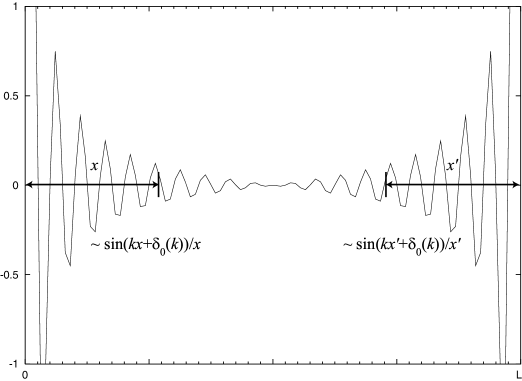
Figure 14: Measuring s-wave phase shifts from the asymptotic form of scattering states in a periodic box of length $L$. The center of the potential is at $x=0$ and $x=L$

Before using this technique for our actual neutron system, we first test our technique for hard sphere scattering where the exact result for the s-wave phase shifts is well known.  If the spheres have radii $r/2$ (therefore the centers of the spheres are separated by $r$) then the s-wave phase shift has the form

$$\delta_{0}=-kr,$$ (115)

where $k$ is the momentum.  The momentum $k$ for a given scattering state can be determined from the energy and the free particle non-relativistic dispersion relation.  In Table 3 we show results for the s-wave phase shift $\delta_{0}$ at inverse lattice spacing $a^{-1}=150$ MeV, with particle masses set at $m_{N}$ and a lattice volume of $20^{3}$.  We use several radii $r$ and show comparisons with the exact continuum result $-kr$.  The results suggest that our lattice Schrödinger technique seems to be functioning properly.

4.50.117−0.56−0.535.50.147−0.85−0.816.50.179−1.20−1.16FRACOPTable 3:  Hard sphere scattering phase shiftsfragments 4.50.117fragments0.56fragments0.535.50.147fragments0.85fragments0.816.50.179fragments1.20fragments1.16\genfrac{}{}{0.0pt}{}{\text{Table 3: \ Hard sphere scattering phase shifts}}{\begin{tabular}[c]{|l|l|l|l|}\hline\cr$r$&$k$&$\delta_{0}$&$-kr$\\ \hline\cr$4.5$&$0.117$&$-0.56$&$-0.53$\\ \hline\cr$5.5$&$0.147$&$-0.85$&$-0.81$\\ \hline\cr$6.5$&$0.179$&$-1.20$&$-1.16$\\ \hline\cr\end{tabular}}

rkδ0-krrkδ0-kr

We now use the lattice Schrödinger technique to tune the coupling $C$ to reproduce the large scattering length that is observed in nature.  In Table 4 we show the best fit values for $C^{phys}$ for several different lattice spacings.

150 MeV−4.0⋅10−5 MeV−2200 MeV−3.4⋅10−5 MeV−2250 MeV−3.1⋅10−5 MeV−2300 MeV−2.9⋅10−5 MeV−2FRACOPTable 4: superscript𝐶𝑝ℎ𝑦𝑠 for different lattice spacingsfragments fragments150 MeVfragments4.0⋅105 MeV2fragments200 MeVfragments3.4⋅105 MeV2fragments250 MeVfragments3.1⋅105 MeV2fragments300 MeVfragments2.9⋅105 MeV2\genfrac{}{}{0.0pt}{}{\text{Table 4: \ }C^{phys}\text{ for different lattice spacings}}{\begin{tabular}[c]{|l|l|}\hline\cr$a^{-1}$&$C^{phys}$\\ \hline\cr$150$\ MeV&$-4.0\cdot 10^{-5}$ MeV${}^{-2}$\\ \hline\cr$200$\ MeV&$-3.4\cdot 10^{-5}$ MeV${}^{-2}$\\ \hline\cr$250$\ MeV&$-3.1\cdot 10^{-5}$ MeV${}^{-2}$\\ \hline\cr$300$\ MeV&$-2.9\cdot 10^{-5}$ MeV${}^{-2}$\\ \hline\cr\end{tabular}}

a-1Cphysa-1Cphys

We can compare this with the pionless case where the only interaction is the contact interaction.  In this case we need only sum bubble diagrams and that gives the relation $C^{phys}\propto a$.  The pionless calculation on the lattice has been discussed in Beane:2003da .

XVII Zone determinant method

It can be shown that fermions at inverse temperature $\beta$ with spatial hopping parameter $h^{\prime}$ have a localization length Lee:2003a of

$$l\sim\sqrt{\beta h^{\prime}}.$$ (116)

This idea was used in Lee:2003mb to generate an algorithm called the zone determinant method to speed up the calculation of determinants using LU decomposition in nuclear lattice simulations.

The technique is relatively simple to describe.  Let $M$ be the neutron matrix, in general an $n\times n$ complex matrix.  We partition the lattice spatially into separate zones such that the length of each zone is larger than the localization length $l$.  Since most neutron worldlines do not cross the zone boundaries, they would not be affected if we set the zone boundary hopping terms to zero.  Hence we anticipate that the determinant of $M$ can be approximated by the product of the submatrix determinants for each spatial zone.

Let us partition the lattice into spatial zones labelled by index $j.$  Let $\{P_{j}\}$ be a complete set of matrix projection operators that project onto the lattice sites within spatial zone $j$.  We can write

$$M=\sum_{i,j}P_{j}MP_{i}=M_{0}+M_{E},$$ (117)

where

$$M_{0} =\sum_{i}P_{i}MP_{i},$$ (118)

$$M_{E} =\sum_{i\neq j}P_{j}MP_{i}.$$ (119)

If the zones can be sorted into even and odd sets so that

$$P_{j}MP_{i}=0$$ (120)

whenever $i$ is even and $j$ is odd or vice-versa, then we say that the zone partitioning is bipartite.  We now have

$$\det(M) =\det(M_{0})\det(1+M_{0}^{-1}M_{E})$$

$$=\det(M_{0})\exp(\text{Tr}(\log(1+M_{0}^{-1}M_{E})))\text{.}$$ (121)

Using an expansion for the logarithm, we have

$$\det(M)=\det(M_{0})\exp\left(\sum_{p=1}^{\infty}\frac{(-1)^{p-1}}{p}\text{Tr}((M_{0}^{-1}M_{E})^{p})\right).$$ (122)

Let us define

$$\Delta_{m}=\det(M_{0})\exp\left(\sum_{p=1}^{m}\frac{(-1)^{p-1}}{p}\text{Tr}((M_{0}^{-1}M_{E})^{p})\right).$$ (123)

Let $\lambda_{k}(M_{0}^{-1}M_{E})$ be the eigenvalues of $M_{0}^{-1}M_{E}$ and $R$ be the spectral radius,

$$R=\max_{k=1,...,n}(\left|\lambda_{k}(M_{0}^{-1}M_{E})\right|).$$ (124)

It has been shown Ipsen:2003 that for $R<1,$

$$\frac{\left|\det(M)-\Delta_{m}\right|}{\left|\Delta_{m}\right|}\leq cR^{m}e^{cR^{m}},$$ (125)

where

$$c=-n\log(1-R).$$ (126)

The spectral radius $R$ determines the convergence of our expansion.  $R$ can be reduced by increasing the size of the spatial zone relative to the localization length $l$.  In the special case where the zone partitioning is bipartite, we note that for any odd $p,$

$$\text{Tr}((M_{0}^{-1}M_{E})^{p})=0.$$ (127)

In that case

$$\Delta_{2m+1}=\Delta_{2m}.$$ (128)

In the simulations presented in this article we use the zone determinant method to calculate neutron matrix determinants.  We use the second order approximation $\Delta_{2}$ with zones of the smallest possible size, a single spatial point ([1,1,1] in the notation of Lee:2003mb ).  An estimate of the approximation error is discussed along with each measurement in the results section.

XVIII Results

We have generated simulation results for $a^{-1}=150$ MeV; $\alpha_{t}=\tfrac{a_{t}}{a}=1.0$; temperatures $T^{phys}=25.0$ MeV and $37.5$ MeV; and lattice sizes $3^{3}$, $4^{4}$, and $5^{5}$.  Half-filling at this lattice spacing occurs at

$$\frac{\rho}{\rho_{N}}=2.64,$$ (129)

where $\rho_{N}^{phys}$ is the normal nuclear density of about $0.17$ nucleons per fm³.  The calculations were performed using the zone determinant method using the second order approximation $\Delta_{2}$ with zones consisting of a single spatial point.  By calculating the exact determinants of some generated matrix configurations we estimate the systemic error for the zone expansion to be about $<0.1\%$ for $T^{phys}=37.5$ MeV and $<0.5\%$ for $T^{phys}=25.0$ MeV.

We have dealt with the complex action by computing the phase as an observable,

$$\left\langle O\right\rangle=\frac{\sum_{[n]}O[n]e^{-\operatorname{Re}S[n]}e^{-i\operatorname{Im}S[n]}}{\sum_{[n]}e^{-\operatorname{Re}S[n]}e^{-i\operatorname{Im}S[n]}}.$$ (130)

For the various simulations presented here we found an average phase of about

$$\frac{\sum_{[n]}e^{-\operatorname{Re}S[n]}e^{-i\operatorname{Im}S[n]}}{\sum_{[n]}e^{-\operatorname{Re}S[n]}}\sim 0.95-1.00,$$ (131)

and so this did not present a significant computational problem.

Figure 15: Energy per nucleon in MeV for temperatures 25 MeV and 37.5 MeV and different lattice volumes.

In Fig. 15 we show the energy per neutron as a function of neutron density.  Our results indicate a rather flat function for the energy per neutron as a function of density.  For comparison we show in Fig. 16 the energy per neutron for the free neutron for temperatures $T^{phys}=7.5$, $15.0$, $25.0$, and $37.5$ MeV.

Figure 16: Energy per nucleon in MeV for temperatures 7.5, 15, 25 and 37.5 MeV and lattice volume $4^{3}$.

In Figs. 17 and 18 we compare with results for free neutrons on the lattice and loop calculations for the physical values of $g_{A}$ and $C$.  As is easily seen, the loop calculations are not very close to the non-perturbative simulation results for the densities shown.

Figure 17: Energy per neutron for temperature $37.5$ MeV and comparisons with the free neutron result on the lattice and loop calculations.

Figure 18: Energy per neutron for temperature $25.0$ MeV and comparisons with the free neutron result on the lattice and loop calculations.

The flatness of our energy per neutron curves at these temperatures are intriguing and hopefully will be checked by others in the near future.  Our results appear to be consistent with the neutron matter results of Muller:1999cp at the same temperatures. Variational calculations Friedman:1981qw and recent quantum Monte Carlo results from Carlson:2003wm observe a gradually flattening of the energy per neutron curve with increasing density, though not as flat as the results we see.  The calculations in Carlson:2003wm however were performed at zero temperature and at lower densities.

We implemented a temporally-improved action in order to remove as much as possible the dependence on $\alpha_{t}=\tfrac{a_{t}}{a}$, the ratio of the temporal lattice spacing to the spatial lattice spacing.  In Fig. 19 we show the dependence on $\alpha_{t}$ for $\alpha_{t}=1.0$, $0.667$, $0.500$.  We see that the dependence on $\alpha_{t}$ is minimal.

Figure 19: Dependence on $\alpha_{t}$ for temperature $37.5$ MeV.

We now look at how the energy per neutron changes as the interaction strength is varied.  According to Table 4, the physical value for $C^{phys}$ at $a^{-1}=150$ MeV is $-4.0\cdot 10^{-5}$ MeV^-2.  If we however take the coupling to be $50\%$, $100\%$, and $150\%$ of the physical value we find the results shown in Fig. 20.

Figure 20: Dependence on $C^{phys}$ for temperature $37.5$ MeV.

In Figs. 21 and 22 we show density versus chemical potential and comparisons with the free neutron and loop calculations.  We can see again that loop calculations are not close to the simulation results.  For fixed chemical potential, the simulation density is higher than the loop-calculated density, which is in turn higher than the free neutron density.

Figure 21: Density versus chemical potential for temperature $37.5$ MeV.

Figure 22: Density versus chemical potential for temperature $25.0$ MeV.

If our effective field theory formalism is valid, we should be able to reproduce the same results for different lattice spacings.  There are however practical computational constraints on $a$.  The determinant zone expansion for fixed zone size and expansion order will break down if the lattice spacing is too small.  For $a^{-1}=200$ MeV we estimate that the second order approximation $\Delta_{2}$ with zones consisting of a single spatial point produces errors of size roughly $3\%$.  In Fig. 23 we compare the energy per neutron as measured for $a^{-1}=150$ MeV and $a^{-1}=200$ MeV at temperature $37.5$ MeV.  The results are in rather good agreement.  In the future we hope to use larger zone sizes and do simulations at lattice spacings up to $a^{-1}=300$ MeV.

Figure 23: Comparison of the energy per neutron results for $a^{-1}=150$ MeV and $a^{-1}=200$ MeV at temperature $37.5$ MeV.

XIX Summary and future directions

We have introduced a new approach to the study of nuclear and neutron matter which combines chiral effective field theory and lattice methods.  Nucleons and pions are treated on the lattice as point particles and we are able to probe larger volumes, lower temperatures, and greater nuclear densities than in lattice QCD.  The low energy interactions of these particles are governed by chiral effective field theory and operator coefficients are determined by fitting to nucleon scattering data.  Any dependence on the lattice spacing can be absorbed by the renormalization of operator coefficients.  In this way we have a realistic simulation of many-body nuclear phenomena with no free parameters, a systematic expansion, and a clear theoretical connection to QCD.  We have presented results for the energy per neutron for hot neutron matter at temperatures 20 to 40 MeV and densities below twice nuclear matter density.

In conjunction with other members of the Nuclear Lattice Collaboration, we plan several extensions, generalizations, and improvements upon this work.  In the course of producing data for this article, we have also generated a large amount of data for the neutral pion, neutron, and pair density correlation functions.  This data will be analyzed and presented in a forthcoming article. In the near future we also plan to study the pionless version of the same neutron system.  There has been a recent mean-field discussion of this model Chen:2003vy .  Without pions, the phase will be completely eliminated from the matrix determinant.  This is due to the fact that the matrix is purely real, and in the Hubbard-Stratonovich formalism the up and down spins appear in a way that the matrix determinant is the square of a real number.  We also plan to extend our studies to include neutrons, protons, neutral and charged pions, and make use the recent progress in implementing exact non-linear representations of chiral symmetry on the lattice Chandrasekharan:2003wy Borasoy:2003pg Lewis:2000cc Shushpanov:1998ms .

References

• (1) H. A. Bethe, Ann. Rev. Nucl. Sci. 21, 93 (1971).
• (2) J. Carlson, J. Morales, J., V. R. Pandharipande, and D. G. Ravenhall, Phys. Rev. C68, 025802 (2003), nucl-th/0302041.
• (3) R. B. Wiringa and S. C. Pieper, Phys. Rev. Lett. 89, 182501 (2002), nucl-th/0207050.
• (4) S. C. Pieper, K. Varga, and R. B. Wiringa, Phys. Rev. C66, 044310 (2002), nucl-th/0206061.
• (5) J. Carlson and R. Schiavilla, Rev. Mod. Phys. 70, 743 (1998).
• (6) B. S. Pudliner, V. R. Pandharipande, J. Carlson, S. C. Pieper, and R. B. Wiringa, Phys. Rev. C56, 1720 (1997), nucl-th/9705009.
• (7) B. S. Pudliner et al., Phys. Rev. Lett. 76, 2416 (1996), nucl-th/9510022.
• (8) S. Weinberg, Phys. Lett. B251, 288 (1990).
• (9) S. R. Beane, P. F. Bedaque, W. C. Haxton, D. R. Phillips, and M. J. Savage, (2000), nucl-th/0008064.
• (10) P. F. Bedaque and U. van Kolck, Ann. Rev. Nucl. Part. Sci. 52, 339 (2002), nucl-th/0203055.
• (11) N. Kaiser, S. Fritsch, and W. Weise, Nucl. Phys. A697, 255 (2002), nucl-th/0105057.
• (12) M. Lutz, B. Friman, and C. Appel, Phys. Lett. B474, 7 (2000), nucl-th/9907078.
• (13) R. Seki, U. van Kolck, and M. J. Savage, Singapore, Singapore: World Scientific (1998) 274 p.
• (14) R. Brockmann and J. Frank, Phys. Rev. Lett. 68, 1830 (1992).
• (15) J. D. Walecka, Annals Phys. 83, 491 (1974).
• (16) H. M. Müller, S. E. Koonin, R. Seki, and U. van Kolck, Phys. Rev. C61, 044320 (2000), nucl-th/9910038.
• (17) W. L. Qian and R.-K. Su, (2002), nucl-th/0210008.
• (18) T. T. S. Kuo, S. Ray, J. Shamanna, and R. K. Su, Int. J. Mod. Phys. E5, 303 (1996), nucl-th/9505025.
• (19) S. Ray, J. Shamanna, and T. T. S. Kuo, Phys. Lett. B392, 7 (1997), nucl-th/9608025.
• (20) J. Pan and S. Das Gupta, Phys. Rev. C57, 1839 (1998), nucl-th/9711003.
• (21) S. Weinberg, Nucl. Phys. B363, 3 (1991).
• (22) D. B. Kaplan, M. J. Savage, and M. B. Wise, Nucl. Phys. B478, 629 (1996), nucl-th/9605002.
• (23) S. R. Beane, P. F. Bedaque, M. J. Savage, and U. van Kolck, Nucl. Phys. A700, 377 (2002), nucl-th/0104030.
• (24) G. P. Lepage, (1997), nucl-th/9706029.
• (25) S. Weinberg, Phys. Lett. B295, 114 (1992), hep-ph/9209257.
• (26) C. Ordonez, L. Ray, and U. van Kolck, Phys. Rev. C53, 2086 (1996), hep-ph/9511380.
• (27) M. Creutz, Found. Phys. 30, 487 (2000), hep-lat/9905024.
• (28) P. Hasenfratz and F. Karsch, Phys. Lett. B125, 308 (1983).
• (29) P. Hasenfratz and F. Karsch, Phys. Rept. 103, 219 (1984).
• (30) M. Creutz, Phys. Rev. D38, 1228 (1988).
• (31) J. E. Hirsch, Phys. Rev. B28, 4059 (1983).
• (32) A. Funk and H. V. von Geramb, (2000), nucl-th/0010058.
• (33) M. Lüscher, Nucl. Phys. B354, 531 (1991).
• (34) M. Lüscher, Commun. Math. Phys. 105, 153 (1986).
• (35) S. R. Beane, P. F. Bedaque, A. Parreno, and M. J. Savage, (2003), hep-lat/0312004.
• (36) D. Lee and P. Maris, Phys. Rev. D67, 076002 (2003).
• (37) D. J. Lee and I. C. F. Ipsen, Phys. Rev. C68, 064003 (2003), nucl-th/0308052.
• (38) I. C. Ipsen and D. Lee, Determinant approximations, Submitted for publication, 2003.
• (39) B. Friedman and V. R. Pandharipande, Nucl. Phys. A361, 502 (1981).
• (40) J.-W. Chen and D. B. Kaplan, (2003), hep-lat/0308016.
• (41) S. Chandrasekharan, M. Pepe, F. D. Steffen, and U. J. Wiese, (2003), hep-lat/0306020.
• (42) B. Borasoy, R. Lewis, and P.-P. A. Ouimet, (2003), hep-lat/0310054.
• (43) R. Lewis and P.-P. A. Ouimet, Phys. Rev. D64, 034005 (2001), hep-ph/0010043.
• (44) I. A. Shushpanov and A. V. Smilga, Phys. Rev. D59, 054013 (1999), hep-ph/9807237.