Gamow and R-matrix Approach to Proton Emitting Nuclei

Abstract

Proton emission from deformed nuclei is described within the non-adiabatic weak coupling model which takes into account the coupling to $\gamma$-vibrations around the axially-symmetric shape. The coupled equations are derived within the Gamow state formalism. A new method, based on the combination of the R-matrix theory and the oscillator expansion technique, is introduced that allows for a substantial increase of the number of coupled channels. As an example, we study the deformed proton emitter ¹⁴¹Ho.

I Introduction

Theoretical models applied to the description of non-spherical proton emitters can be divided into two groups. The core-plus-particle models describe the radioactive parent nucleus in terms of a single proton interacting with a core (i.e., the daughter nucleus). Usually, the core is represented by some phenomenological collective model, e.g., the Bohr-Mottelson (geometric) model. Depending on the structure of the daughter nucleus, rotational kru00 ; bar00 ; es01 or vibrational dav01 ; hag01 couplings are assumed. The models belonging to this group employ the coupled-channel formalism of reaction theory which has been developed in the context of elastic or inelastic scattering.

Models belonging to the second group employ the framework of the deformed shell model. In the simplest case, the proton resonance corresponds to a Nilsson state of a deformed mean field kad96 ; fer97 ; mag98 ; dav98 ; mag99 ; ryk99 ; son99 . Approaches belonging to this group can be generalized to include the BCS pairing fio03 .

We may refer to the first group of models as weak-coupling models or coupled-channel models. For the second group of models, we reserve the term resonance Nilsson-orbit (or adiabatic) models. The term “adiabatic” requires an explanation. It is very difficult to relate both groups of models to each other, because they operate on different approximation levels. In special situations, however, this relationship can be revealed. For instance, in the limit of the infinite moment of inertia of the axial weak-coupling model (which implies degenerate rotational bands and strong rotational coupling BMII ), one recovers the resonance Nilsson-orbit model kru03 . So one may say that in this case the adiabatic model is an approximation to the weak-coupling (non-adiabatic) picture. Generally, however, the relation between adiabatic and non-adiabatic descriptions is not simple. For example, the resonance Nilsson-orbit model with a triaxial potential dav03a (i.e., nonzero $\gamma$ deformation) cannot be trivially related to a weak-coupling model extended to triaxial degrees of freedom kru03 .

If the coupled-channel model with the rotational coupling is applied to the nucleus ¹⁴¹Ho, the ground-state decay characteristics (half-life time and branching ratio) are poorly described bar00 ; es01 . There are several explanations possible. For example, it may be that the Coriolis mixing is too strong es01 . This can be partly cured if pairing is introduced fio03 . Another possibility, explored in this work, is the coupling to triaxial vibrations. Indeed, in particle-plus-rotor calculations, the best description of the experimentally observed band structures of ¹⁴¹Ho can be explained if $\gamma$ deformation is considered sew01 . In addition, in the neighboring nuclei, such as ¹³⁶Sm and ¹⁴⁰Gd, there are low-lying $2^{+}_{2}$ and $3^{+}$ levels ensdf which have been interpreted wal01 as members of a $\gamma$-vibrational band. There are also other indications that in this mass region the coupling to triaxial modes can play a role yan93 ; kor90 . The possibility that triaxiality influences the decay of ¹⁴¹Ho was investigated in our earlier work kru03 and also in the recent Refs. dav03a ; dav03 based on an adiabatic model assuming a triaxially deformed mean field.

In this work, we present non-adiabatic calculations in which the excitations of the daughter nucleus are properly taken into account. Unlike in Ref. dav03 , we do not assume a permanent $\gamma$ deformation of the core, but rather we consider $\gamma$ vibrations around the axially-symmetric deformed shape.

The ground-state rotational band of ¹⁴⁰Dy has recently been observed kro02 ; cul02 . In addition, in our work we assume that ¹⁴⁰Dy has the $K$=2 $\gamma$-vibrational band. This structure can be coupled to the ground-state band if the proton-daughter interaction in the body-fixed system deviates from the axial symmetry. The experimentally observed rotational band of the parent nucleus is assumed to be a $K^{\pi}$=7/2^- band sew01 built upon the [523]_Ω=7/2 Nilsson level. In the strong-coupling picture the presence of the $\gamma$ band in ¹⁴⁰Dy implies the existence of two additional rotational bands in ¹⁴¹Ho with $K$=$\Omega\pm 2$, i.e., $K^{\pi}=3/2^{-}$ and $K^{\pi}=11/2^{-}$.

In the weak-coupling model, proton emission is described by means of a coupled set of differential equations which are solved assuming appropriate boundary conditions. The most obvious way to describe the proton emission is to assume outgoing boundary conditions. This immediately leads to the notion of the Gamow or resonant states, the generalized eigenstates of the time-independent Schrödinger equation, which are regular at the origin and satisfy purely outgoing boundary conditions. Together with non-resonant scattering states, Gamow states form a complete set, the so-called Berggren ensemble berggren , which can be used in a variety of applications vertse87 , including the recently developed Gamow shell model Mic02 ; Mic03 ; betan .

Unfortunately, the number of coupled equations rapidly increases with the number of excited states of the daughter nucleus taken into account. In addition, the solution of the eigenvalue problem of a very large set of coupled equations becomes numerically unstable at some point. This is especially true if one keeps in mind that there is a twenty-order-of-magnitude difference between the real and imaginary part of the energy of the Gamow-state which describes the proton decay of ¹⁴¹Ho. A possible way out is to consider the R-matrix theory. However, even in this case, one has to deal with large sets of coupled differential equations.

In order to avoid the difficulty of solving large sets of coupled differential equations, one may use the Rayleigh-Ritz variational principle and apply the basis expansion method. In this paper, the spherical harmonic oscillator wave functions are used as basis functions. It was recognized a long time ago that by using the basis expansion method the positions of narrow resonances can be determined. In particular, the signature of a narrow resonance is that the specific positive energy solution is locally stable with respect to the change of the size of the basis Haz70 ; Rei79 ; Lov82 ; Man93 ; sal96 ; Kru99 ; Ara99 ; kruppa00 . Several proposals exist in the literature on how to determine the width of the resonance in this method. They are called $L^{2}$ stabilization methods sal96 . (The name comes from the fact that only square integrable functions are used in the expansion.) In this paper we will introduce a new method which is a combination of the oscillator expansion method and the R-matrix formalism. This method is very simple and proves to be accurate enough for very narrow proton resonances.

The paper is organized as follows. We begin in Sec. II with an overview of the weak-coupling model applied to the case of rotational motion and $\gamma$ vibrations. Section III reviews different methods to calculate the position and width of a resonance state: the theory of Gamow-states, the standard R-matrix formalism, and the new method which combines the oscillator expansion method with the R-matrix formalism. Finally, Sec. IV contains results of numerical calculations. We check the accuracy of the new method and demonstrate how the position of excited states in the daughter nucleus can influence predictions of the weak-coupling model. We also present results for the proton emission in ¹⁴¹Ho. Finally, Sec. V contains the conclusions of this work.

II Weak-coupling model

The proton-emitting parent nucleus is described here in terms of a single proton coupled to a deformed core. The model Hamiltonian can be written as

$$H_{\rm rot}=H_{\rm d}-\frac{\hbar^{2}}{2m}\bigtriangleup_{\bf r}+V_{\rm def}({\bf r},\omega),$$ (1)

where $H_{\rm d}$ is the (collective) Hamiltonian of the daughter nucleus, the second term represents the relative proton-daughter kinetic energy, and $V_{\rm def}$ is the proton-core interaction, which depends on the position of the proton ${\bf r}$ and the orientation $\omega$ of the core.

II.1 The proton-daughter interaction

It is straightforward to define $V_{\rm def}$ in the body-fixed frame, in which one can define the deformed mean field. By expanding the nuclear radius in multipoles and assuming quadrupole deformations only, one obtains

$$R(\theta^{\prime},\phi^{\prime})=R_{0}C(a_{0},a_{2})\left[1+a_{0}Y_{2,0}(\theta^{\prime})+a_{2}(Y_{2,2}(\theta^{\prime},\phi^{\prime})+Y_{2,-2}(\theta^{\prime},\phi^{\prime}))\right]$$ (2)

where $C(a_{0},a_{2})$ is the volume conservation factor. The intrinsic deformed field is defined using a Saxon-Woods form factor

$$V_{\rm def}(r,\theta^{\prime}\phi^{\prime})=-\frac{V_{0}}{1+\exp\left[(r-R(\theta^{\prime},\phi^{\prime}))/a\right]}.$$ (3)

Expanding to the first order in $a_{2}$, one obtains

$$V_{\rm def}(r,\theta^{\prime}\phi^{\prime})=V_{1}(r,\theta^{\prime})+a_{2}V_{2}(r,\theta^{\prime})\left[Y_{2,2}(\theta^{\prime},\phi^{\prime})+Y_{2,-2}(\theta^{\prime},\phi^{\prime})\right].$$ (4)

The form factor $V_{1}(r,\theta^{\prime})$ is the same as (3) except that $a_{2}$ is put equal to zero. The form factor of the second term is given by

$$V_{2}(r,\theta^{\prime})=-\frac{V_{0}R(\theta^{\prime},\phi^{\prime})e^{{r-R(\theta^{\prime},\phi^{\prime})}\over a}}{a\left[1+e^{{r-R(\theta^{\prime},\phi^{\prime})}\over a}\right]^{2}},$$ (5)

where, again, $a_{2}$=0 in $R(\theta^{\prime},\phi^{\prime})$. The deformed form factors $V_{1}(r,\theta^{\prime})$ and $V_{2}(r,\theta^{\prime})$ still depend on $a_{0}$. After perfoming multipole decomposition of $V_{1}$ and $V_{2}$, one obtains the intrinsic potential:

$$V_{\rm def}(r,\theta^{\prime}\phi^{\prime})=V^{(1)}_{\rm def}(r,\theta^{\prime})+a_{2}V^{(2)}_{\rm def}(r,\theta^{\prime}\phi^{\prime})$$

$$=\sum_{\lambda}V_{\lambda}^{(1)}(r)Y^{\prime}_{\lambda,0}(\theta^{\prime})+a_{2}\sum_{\lambda}V_{\lambda}^{(2)}(r)\left[Y^{\prime}_{\lambda,2}(\theta^{\prime},\phi^{\prime})+Y^{\prime}_{\lambda,-2}(\theta^{\prime},\phi^{\prime})\right].$$ (6)

For explicit expressions for $V_{\lambda}^{(1)}(r)$ and $V_{\lambda}^{(2)}(r)$ see, e.g., Ref. ta65 . It can be shown that in the laboratory system the daughter-proton interaction is given by

$$V_{\rm def}({\bf r},\omega)=V_{\rm def}^{(1)}({\bf r},\omega)+a_{2}V_{\rm def}^{(2)}({\bf r},\omega)$$

$$=\sum_{\lambda\mu}V_{\lambda}^{(1)}(r)D^{\lambda}_{\mu 0}Y_{\lambda,\mu}(\hat{r})+a_{2}\sum_{\lambda\mu}V_{\lambda}^{(2)}(r)\left(D^{\lambda}_{\mu 2}+D^{\lambda}_{\mu-2}\right)Y_{\lambda,\mu}(\hat{r}).$$ (7)

In addition to the nuclear potential, there is also a long-range Coulomb interaction between the deformed core and the proton. The deformed Coulomb form factors, $V_{C}^{(1)}$ and $V_{C}^{(2)}$, are discussed in Appendix A.

II.2 The coupled channel equations

The states of the daughter nucleus are eigenvectors of $H_{\rm d}$. In this work, we adopt the rotational-vibrational collective model. The wave functions of the core, $\phi_{I\mu K}$, are given by the standard ansatz BMII :

$$\phi_{I\mu K}=\sqrt{\frac{2I+1}{16\pi^{2}(\delta_{K,0}+1)}}\left[D^{I*}_{\mu K}+(-1)^{I}D^{I*}_{\mu-K}\right]\chi_{Kn_{2}}(a_{2})|{\rm g.s.}\rangle,$$ (8)

where $\chi_{Kn_{2}}(a_{2})$ is a $\gamma$-vibrational wave function. The wave function of the parent nucleus can be written in the weak-coupling form

$$\Psi^{JM}=\sum_{IKlj}\frac{u^{J}_{IKlj}(r)}{r}\Phi_{JMIKlj},$$ (9)

where the channel function is given by

$$\Phi_{JMIKlj}=\sum_{\Omega\mu}\langle j\Omega I\mu|JM\rangle{\cal Y}_{lj\Omega}\phi_{I\mu K},$$ (10)

and

$${\cal Y}_{lj\Omega}=\sum_{ms}\langle lm\frac{1}{2}s|j\Omega\rangle i^{l}Y_{lm}(\hat{r})\chi_{1/2}(s)$$ (11)

arises from the coupling of the proton spin with the orbital angular momentum. In our earlier weak-coupling calculations kru00 ; bar00 there was no summation over $K$ in Eq. (9); only the $K=0$ term was considered. Due to the non-axial symmetric form of the proton-daughter interaction (II.1), the ground state $K=0$ and the $\gamma$-vibrational $K=2$ band both contribute.

The radial functions $u^{J}_{IKlj}(r)$ are solutions of the set of coupled-channel equations:

$$\frac{\hbar^{2}}{2m}\left(-\frac{d^{2}}{dr^{2}}+\frac{l(l+1)}{r^{2}}\right)u^{J}_{IKlj}+\sum_{\lambda I^{\prime}l^{\prime}j^{\prime}}A_{\lambda}(Ilj,I^{\prime}l^{\prime}j^{\prime},J)B_{\lambda}(II^{\prime}K)V_{\lambda}^{(1)}u^{J}_{I^{\prime}Kl^{\prime}j^{\prime}}+$$ (12)

$$\sum_{\lambda I^{\prime}K^{\prime}l^{\prime}j^{\prime}}A_{\lambda}(Ilj,I^{\prime}l^{\prime}j^{\prime},J)C_{\lambda}(IKI^{\prime}K^{\prime},a_{2})V_{\lambda}^{(2)}u^{J}_{I^{\prime}K^{\prime}l^{\prime}j^{\prime}}=(E-E_{IK})u^{J}_{IKlj},$$

where $E_{IK}$ is the energy of the daughter state described by the wave function (8). The $r$-independent coupling coefficients can be written in terms of the reduced nuclear matrix elements

$$B_{\lambda}(II^{\prime}K)=\langle\phi_{IK}||D^{\lambda}_{;0}||\phi_{I^{\prime}K}\rangle$$ (13)

and

$$C_{\lambda}(IKI^{\prime}K^{\prime},a_{2})=\langle\phi_{IK}||a_{2}(D^{\lambda}_{;2}+D^{\lambda}_{;-2})||\phi_{I^{\prime}K^{\prime}}\rangle.$$ (14)

The explicit expressions for the geometric coefficients $A_{\lambda}(Ilj,I^{\prime}l^{\prime}j^{\prime},J)$ are given, e.g., in Ref. tam65 . The nuclear structure model of the daughter nucleus enters the formalism through the reduced matrix elements $B_{\lambda}$ and $C_{\lambda}$ tam65 ; ta65 .

III Calculation of resonance parameters

The coupled differential equations (12) can be turned into an eigenvalue problem by specifying boundary conditions. It is always assumed that the solutions are regular at the origin, i.e., $u_{c}(0)=0$. (From now on, the channel indexes $IKlj$ are abbreviated by the symbol $c$.)

III.1 Gamow states

To be a Gamow state, the radial wave function must asymptotically behave as an outgoing Coulomb wave:

$$u_{c}(r) \stackrel{{\scriptstyle{\rm large}\;r}}{{\longrightarrow}} O_{l}(\eta,rk_{p})$$ (15)

$$= G_{l}(\eta,rk_{p})+iF_{l}(\eta,rk_{p}),$$

where $k^{2}_{c}=\frac{2m}{\hbar^{2}}({\cal E}_{p}-E_{IK})$ and $\eta k_{c}=\frac{m}{\hbar^{2}}Ze^{2}$. Such boundary conditions are only satisfied for a discrete set of complex wave numbers $k_{c}$ which define the generalized eigenvalues $E={\cal E}_{p}$ of Eq. (12). These eigenvalues correspond to the poles of the scattering matrix [Hum61] ; vertse87 . The corresponding solutions are either bound states with negative real energies ${\cal E}_{p}=E_{b}<0$ and pure imaginary wave numbers $k_{p}=i\gamma_{p}$ ($\gamma_{p}>0$), or resonance states, ${\cal E}_{p}=E_{\rm res}-i\frac{\Gamma_{\rm res}}{2}$, with nonzero imaginary parts $\Gamma_{\rm res}\neq 0$, and $k_{p}=\kappa_{p}-i\gamma_{p}$.

The asymptotic behavior of the radial wave functions are determined by $k_{p}$. For Gamow states these functions show oscillating behavior at large values of $r$ so one must define a new normalization scheme. Berggren proposed berggren a generalized scalar product and introduced a regularization procedure (${{\cal R}eg}$). With this generalization the norm is

$$\sum_{c}{{\cal R}eg}\int_{0}^{\infty}[u_{c}(r)]^{2}\,dr=1.$$ (16)

Once the resonance energy and radial wave function have been determined, there are different methods to calculate the width of the state. The simplest method is to take twice the imaginary part of the energy of the resonance. However, for narrow resonances the accurate numerical calculation of ${\cal I}{\rm m}[{\cal E}_{p}]$ is difficult. Therefore, other methods are often used. One possibility is to calculate the partial width for each channel from the so-called current expression [Hum61]

$$\Gamma_{c}(r)=i\frac{\hbar^{2}}{2\mu}\frac{u_{c}^{\prime*}(r)u_{c}(r)-u^{\prime}_{c}(r)u_{c}^{*}(r)}{\sum_{c^{\prime}}\int_{0}^{r}|u_{c^{\prime}}(r^{\prime})|^{2}{\rm d}r^{\prime}},$$ (17)

where the sum of the partial widths

$$\Gamma_{\rm res}=\sum_{c}\Gamma_{c}(r)$$ (18)

gives the total decay width. Although values of $\Gamma_{c}(r)$ depend on $r$ in the region where the coupling potential terms are not negligible, the total width (18) is independent of $r$, which reflects flux conservation.

In practice, the Gamow boundary condition given by Eq. (15) can be implemented in the form

$$\frac{u^{\prime}_{c}(r_{\rm as})}{u_{c}(r_{\rm as})}=k_{p}\frac{O^{\prime}_{l}(\eta,r_{\rm as}k_{p})}{O_{l}(\eta,r_{\rm as}k_{p})},$$ (19)

where $r_{\rm as}$ is the channel radius (the off-diagonal couplings are negligible for $r>r_{as}$). Using Eq. (19), the partial decay width can be written at the point $r_{as}$ as

$$\Gamma_{c}(r_{\rm as}) = i\frac{\hbar^{2}}{2\mu}\frac{|u_{c}(r_{\rm as})|^{2}}{|O_{l}(\eta,k_{p}r_{\rm as})|^{2}\sum_{c^{\prime}}\int_{0}^{r_{\rm as}}|u_{c^{\prime}}(r^{\prime})|^{2}{\rm d}r^{\prime}}$$ (20)

$$\times \left[k_{p}^{*}O^{\prime*}_{l}(\eta,r_{\rm as}k_{p})O_{l}(\eta,r_{\rm as}k_{p})-k_{p}O^{\prime}_{l}(\eta,r_{\rm as}k_{p})O^{*}_{l}(\eta,r_{\rm as}k_{p})\right].$$

If one neglects the imaginary part of $k_{p}$, the square bracket in Eq. (20) becomes $-2i$ and the expression for the partial decay width can be written in a simple form:

$$\Gamma_{c}(r_{\rm as})\approx\frac{\hbar^{2}\kappa_{p}}{\mu}\frac{|u_{c}(r_{\rm as})|^{2}}{|O_{l}(\eta,k_{p}r_{\rm as})|^{2}\sum_{c^{\prime}}\int_{0}^{r_{\rm as}}|u_{c^{\prime}}(r^{\prime})|^{2}{\rm d}r^{\prime}}.$$ (21)

Equation (20) and its approximate form (21) are strictly valid only at the point $r_{\rm as}$ where the boundary condition is given. We emphasize at this point that if the coupled equations are solved with the Gamow boundary condition, then the total width can be calculated at any value of $r$ using exact relations (17) and (18).

III.2 R-matrix method

For completeness, we summarize those important aspects of the R-matrix theory La58 which are relevant to our work. In the R-matrix theory one also deals with a set of radial functions $g_{c}(r)$. These functions are regular at the origin and satisfy the same coupled equations (12) as the Gamow states but with the following boundary conditions

$$a\frac{g_{c}^{\prime}(a)}{g_{c}(a)}=B_{c},$$ (22)

where the parameters $B_{c}$ are arbitrary real numbers. It is assumed that the short-range diagonal and off-diagonal proton-core interactions can be neglected beyond the channel radius $a$. Consequently, $a$ has the same meaning as the parameter $r_{\rm as}$ of the Gamow theory. It is worth noting, however, that $a$ is always real, while $r_{\rm as}$ can be complex.

The boundary condition (22) defines the complete set of functions inside the channel surface. The real eigenvalues of the coupled-channel equations are denoted by $E_{\lambda}$ and the corresponding eigenfunctions by $g^{\lambda}_{c}(r)$. They are normalized to one inside the channel surface,

$$\sum_{c}\int_{0}^{a}|g^{\lambda}_{c}(r)|^{2}dr=1,$$ (23)

and define the so-called reduced width amplitudes

$$\gamma_{\lambda c}=\left(\frac{\hbar^{2}}{2m_{c}a}\right)^{1/2}g^{\lambda}_{c}(a).$$ (24)

The resulting R-matrix has a simple form

$$R_{cc^{\prime}}(E)=\sum_{\lambda}\frac{\gamma_{\lambda c}\gamma_{\lambda c^{\prime}}}{E_{\lambda}-E}$$ (25)

but it is related to the physically important scattering S-matrix in a complicated way La58 . Let us emphasize that the calculated S-matrix is independent from both the boundary condition parameters $B_{c}$ and from the channel radius $a$ only if all the R-matrix states are taken into account in Eq. (25).

Assuming that in a given energy region only one term dominates in the R-matrix and making further approximations (see p. 322 of Ref. La58 ), Lane and Thomas showed that the S-matrix can be written in the form

$$S_{cc^{\prime}}(E)\approx S^{0}_{cc^{\prime}}(E)\left[\delta_{c,c^{\prime}}+\frac{i\Gamma_{\lambda c}(E)^{1/2}\Gamma_{\lambda c^{\prime}}(E)^{1/2}}{E_{\lambda}+\Delta_{\lambda}(E)-E-\frac{i}{2}\Gamma_{\lambda}(E)}\right],$$ (26)

where the partial R-matrix widths

$$\Gamma_{\lambda c}(E)=2P_{l_{c}}(E)\gamma_{\lambda c}^{2}$$ (27)

give the total width

$$\Gamma_{\lambda}(E)=\sum_{c}\Gamma_{\lambda c}(E).$$ (28)

In Eq. (26), function $\Delta_{\lambda}(E)$ is given by

$$\Delta_{\lambda}(E)=\sum_{c}\Delta_{\lambda c}(E),$$ (29)

where

$$\Delta_{\lambda c}(E)=-\left(S_{l_{c}}(E)-B_{c}\right)\gamma^{2}_{\lambda c}.$$ (30)

The penetration $P_{l_{c}}(E)$ and shift $S_{l_{c}}(E)$ functions are related to the Coulomb $F_{l_{c}}$ and $G_{l_{c}}$ functions (see p. 270 of Ref. La58 ).

Within approximation (26), the complex-energy resonance poles of the S-matrix, ${\cal E}^{R}_{p}=E^{R}_{\rm res}-\frac{i}{2}\Gamma^{R}_{\rm res}$, satisfy the equation

$$E_{\lambda}+\Delta_{\lambda}({\cal E}^{R}_{p})-{\cal E}^{R}_{p}-\frac{i}{2}\Gamma_{\lambda}({\cal E}^{R}_{p})=0.$$ (31)

Here, we used the upper index $R$ in order to distinguish this R-matrix approximation for the resonance energy from the energy of the corresponding Gamow state. In order to simplify the solution of the non-linear equation (31), one often introduces further approximations and assumptions for the calculation of the functions $\Delta_{\lambda}(E)$ and $\Gamma_{\lambda}(E)$.

In the method of Thomas Th54 , the function $\Delta_{\lambda c}(E)$ is expanded around the R-matrix eigenvalue $E_{\lambda}$

$$\Delta_{\lambda c}(E)\approx-(S_{l_{c}}(E)-B_{c})-\dot{S}_{l_{c}}(E_{\lambda})(E-E_{\lambda}),$$ (32)

where the dot denotes energy derivative. Furthermore, the $E$-dependence of $\Gamma_{\lambda c}(E)$ is neglected and $\Gamma_{\lambda c}(E)$ is replaced by the corresponding value at $E_{\lambda}$. Under these assumptions one obtains

$$E^{R}_{\rm res}=\frac{E_{\lambda}+\sum_{c}\left(B_{c}-S_{l_{c}}(E_{\lambda})\right)\gamma_{\lambda c}^{2}}{1+\sum_{c}\dot{S}_{l_{c}}(E_{\lambda})\gamma_{\lambda c}^{2}}$$ (33)

and

$$\Gamma_{\rm res}^{R}=\frac{\Gamma_{\lambda}(E_{\lambda})}{1+\sum_{c}\dot{S}_{l_{c}}(E_{\lambda})\gamma_{\lambda c}^{2}}.$$ (34)

In order to simplify (33) we may require that the chosen boundary condition parameters satisfy the condition:

$$B_{c}=S_{l_{c}}(E_{\lambda}).$$ (35)

If the $\dot{S}_{l_{c}}(E_{\lambda})$ terms are negligible, then the resonance energy corresponds to the R-matrix eigenvalue

$$E_{\rm res}^{R}=E_{\lambda}$$ (36)

and the width can be calculated with the well-known expression

$$\Gamma_{\rm res}^{R}=\sum_{c}2P_{l_{c}}(E_{\lambda})\gamma_{\lambda c}^{2}.$$ (37)

Two variants of Thomas’s procedure can be found in a later paper of Lane and Thomas La58 where they give different expressions for $E_{\rm res}^{R}$ and $\Gamma_{\rm res}^{R}$.

III.3 R-matrix method using oscillator expansion

In this section we propose a simple method, based on the R-matrix formalism, to estimate the parameters of a resonance. The advantage of this method is that it avoids solving a large set of coupled differential equations. The method is based on the expansion of the radial functions $u_{IKlj}(r)$ in the single-particle basis $\phi^{HO}_{nl}(r)$ of the spherical harmonic oscillator. In this basis, the total wave function (9) can be written in the form:

$$\Psi^{JM}=\sum_{IKlj}\sum_{n}C^{J}_{IKnlj}\frac{\phi^{HO}_{nl}(r)}{r}\Phi_{JMIKlj}.$$ (38)

The coefficients $C^{J}_{IKnlj}$ can be obtained from the matrix eigenvalue equation:

$$\sum_{n^{\prime}}\langle\phi^{HO}_{nl}|\frac{\hbar^{2}}{2m}\left(-\frac{d^{2}}{dr^{2}}+\frac{l(l+1)}{r^{2}}\right)|\phi^{HO}_{n^{\prime}l}\rangle C^{J}_{IKn^{\prime}lj}-(E^{HO}_{\lambda}-E_{IK})C^{J}_{IKnlj}$$

$$+\sum_{\lambda I^{\prime}n^{\prime}l^{\prime}j^{\prime}}A_{\lambda}(Ilj,I^{\prime}l^{\prime}j^{\prime},J)B_{\lambda}(II^{\prime}K)\langle\phi^{HO}_{nl}|V_{\lambda}^{(1)}|\phi^{HO}_{n^{\prime}l^{\prime}}\rangle C^{J}_{I^{\prime}Kn^{\prime}l^{\prime}j^{\prime}}$$ (39)

$$+\sum_{\lambda I^{\prime}K^{\prime}n^{\prime}l^{\prime}j^{\prime}}A_{\lambda}(Ilj,I^{\prime}l^{\prime}j^{\prime},J)C_{\lambda}(IKI^{\prime}K^{\prime},a_{2})\langle\phi^{HO}_{nl}|V_{\lambda}^{(2)}|\phi^{HO}_{n^{\prime}l^{\prime}}\rangle C^{J}_{I^{\prime}K^{\prime}n^{\prime}l^{\prime}j^{\prime}}=0.$$

In the following, the corresponding real eigenvalues are denoted as $E^{HO}_{\lambda}$.

In the R-matrix theory, the coupled equations (12) are solved with imposed boundary conditions (22). However, as discussed in the following, this procedure can be reversed. In the first step, we solve the algebraic eigenvalue problem (III.3) for the coefficients $C^{J}_{IKnlj}$. The resulting radial functions $g_{c}(r)$ define the boundary condition function at the point $r$:

$$B_{c}(r)=B_{IKlj}(r)=r\left(\sum_{n}C^{J}_{IKnlj}\phi^{HO}_{nl}(r)\right)^{\prime}/\sum_{n}C^{J}_{IKnlj}\phi^{HO}_{nl}(r).$$ (40)

Having determined the boundary condition parameter at each $r$, the R-matrix formalism can now be applied. In particular, after replacing $E_{\lambda}$ with $E^{HO}_{\lambda}$ in expressions (33) and (34), they can be used to compute the position and the width of a resonance at each value of $r$:

$$E^{HO}_{\rm res}(r)=\frac{E^{HO}_{\lambda}+\sum_{c}\left(B_{c}(r)-S_{l_{c}}(E_{\lambda}^{HO})\right)\gamma_{\lambda c}(r)^{2}}{1+\sum_{c}\dot{S}_{l_{c}}(E_{\lambda}^{HO})\gamma_{\lambda c}(r)^{2}}$$ (41)

and

$$\Gamma_{\rm res}^{HO}(r)=\frac{\Gamma_{\lambda}(E_{\lambda}^{HO})}{1+\sum_{c}\dot{S}_{l_{c}}(E_{\lambda}^{HO})\gamma_{\lambda c}(r)^{2}},$$ (42)

where the $r$-dependent reduced width amplitudes (24) are given by

$$\gamma_{\lambda c}(r)=\left(\frac{\hbar^{2}}{2m_{c}r}\right)^{1/2}\sum_{n}C^{J}_{IKnlj}\phi^{HO}_{nl}(r).$$ (43)

This algorithm is further referred to as the R-matrix method based on harmonic oscillator expansion (RMHO). In RMHO, the energy and width of the resonance explicitly depend on $r$. However, for sufficiently large values of $r$, this dependence is expected to be extremely weak. It is to be noted that since expression (37) is derived under specific assumption (35), it is not valid in the RMHO method.

The derived boundary condition parameters (40) do not depend on the actual normalization used. However, this is no longer true for the reduced width amplitudes (24). In order to apply the R-matrix method at each $a$=$r$, the radial functions

$$g_{c}(r)=g_{IKlj}(r)=\sum_{n=0}^{n_{\rm max}}C^{J}_{IKnlj}\phi^{HO}_{nl}(r)$$ (44)

have to be renormalized to one inside the channel surface according to Eq. (23).

IV Results

The numerical tests have been carried out for the deformed proton emitter ¹⁴¹Ho, viewed as a proton-plus-core system, with the daughter nucleus ¹⁴⁰Dy being the collective core. We employed the same successful parameterization of the Woods-Saxon (WS) optical potential as in earlier Ref. bar00 .

IV.1 Resonance Width in RMHO

Let us first assume that the core is axially deformed ($a_{2}=0$). In the calculations, all the states in the g.s. rotational band in the daughter nucleus up to $I$=12 were considered. In our weak-coupling calculations, the experimental excitation energies of ¹⁴⁰Dy were used for states with $I$$<$10, and the energies of the remaining states were obtained by the variable-moment-of-inertia (VMI) fit to the data. That is, for the g.s. band we took the values: 0.203, 0.567, 1.044, 1.597, 2.218, and 2.894 MeV. The deformation parameter $a_{0}$ was set to the value of 0.244, which is consistent with earlier investigations sew01 ; kro02 . The WS strength was adjusted to reproduce the experimental position of the $J^{\pi}$=7/2^- resonance at 1.19 MeV. The number of coupled channels in this variant is 46. This number is sufficiently small to carry out the reliable calculation of the Gamow-state energy eigenvalue. The resulting resonance width is ${\rm 0.208\times 10^{-19}}$ MeV. We accept this number as the exact, or reference, value.

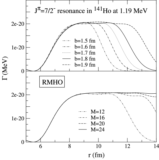
Figure 1: The width of the $J^{\pi}$=7/2^- resonance in ¹⁴¹Ho at 1.19 MeV calculated in RMHO as a function of $r$. Top: dependence on the oscillator length parameter $b$ (the number of basis states is $M$=12). Bottom: dependence on $M$ ($b$=1.8 fm).

The harmonic oscillator basis is characterized by a single parameter, the oscillator length $b$. The upper part of Fig. 1 shows the resonance width (42) calculated in RMHO as a function of $r$. For each partial wave, $M$=$n_{\rm max}$+1=12 harmonic oscillator functions were used in the expansion (44) and the value of $b$ was varied. As expected, a clear plateau appears at large values of $r$. The extent of the plateau depends on the size of $b$: the greater oscillator length (i.e., the r.m.s. oscillator radius), the greater the extent of the plateau. The reason for the rapid decrease of the width function $\Gamma^{HO}_{\rm res}(r)$ at very large values of $r$ lies in the fact that the radial channel function is approximated by a linear combination of a finite number of oscillator functions, each having the Gaussian asymptotic behavior. Therefore, by increasing the number of states in the basis, the extent of the plateau is expected to increase. This is illustrated in Fig. 1 (lower portion) which shows RMHO results obtained at a fixed value of $b$=1.8 fm for several values of $M$. It is seen that for $M$=24 ($n_{\rm max}$=23) the width function becomes independent of $r$ in a very wide interval of $r$. In the interval between $r$=9 and 12 fm the RMHO width exhibits tiny oscillations (practically invisible in Fig. 1). Therefore, to obtain a well-defined value, we divide this interval equidistantly with a step size of 0.1 fm and calculate the average $\bar{\Gamma}^{HO}_{\rm res}=\frac{1}{N_{r}}\sum_{i=1}^{N_{r}}\Gamma^{HO}_{\rm res}(r_{i})$, which will be considered as the RMHO width in the following.

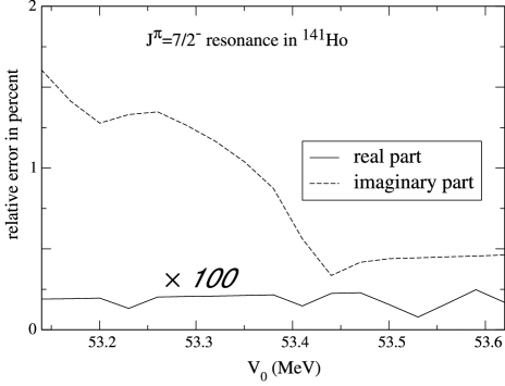
Figure 2: The relative error of the real (solid line) and imaginary (dashed line) energy of the $J^{\pi}$=7/2^- resonance in ¹⁴¹Ho calculated in RMHO ($M$=24) as a function of the WS potential depth $V_{0}$. The reference (exact) values are taken from the Gamow states calculation. In the considered range of $V_{0}$, the resonance width changes by four orders of magnitude. Note that the solid curve has been multiplied by a factor of 100.

In order to assess the quality of the RMHO method, Fig. 2 shows the relative errors of the real and imaginary part of the energy of the resonance as a function of the WS potential depth $V_{0}$. The reference values were obtained by the Gamow-state coupled-channel procedure. In the considered region of $V_{0}$, the resonance width changes by four orders of magnitude; however, the relative error of RMHO is less than 1.7 percent. The accuracy of RMHO for the real part of the energy is much better: the relative error is always smaller than 0.0025 percent. The results presented in Figs. 1 and 2 convincingly demonstrate that the RMHO formalism can be safely used to calculate isolated narrow proton resonances.

IV.2 Proton decay of ¹⁴¹Ho

In this section we investigate the influence of $\gamma$ vibrations on the process of proton emission from ¹⁴¹Ho. All results presented in this section are obtained with the RMHO method using $M$=20 oscillator functions for each partial wave. The oscillator length was assumed to be $b$=1.8 fm. Using the results of the VMI fit for the g.s. band, the assumed energies of the members of the $\gamma$ band are: 0.750, 0.934, 1.144, 1,378, 1.633, 1.907, 2.198, 2.504, 2.825 3.159, and 3.507 MeV for $I=2,3,4,\ldots 12$. The chosen position of the $2^{+}_{2}$ band head of the $\gamma$-vibrational band, 750 keV, was taken according to the systematic trends around $N$=74.

When one includes the $K$=2 $\gamma$-vibrational band in addition to the g.s. band, the number of coupled channels increases from 46 to 130 (assuming that the maximum spin is $I_{\rm max}$=12 in both bands). For that reason, we decided to carry out the RMHO calculations instead of the weak-coupling Gamow analysis. We have checked, however, that for $I_{\rm max}$=10, where the coupled-channel calculations with the $K$=2 band can be done, the RMHO results coincide with those of the coupled-channel method.

IV.2.1 Structure of $J^{\pi}$=7/2^- states

The simplest model of the g.s. decay of ¹⁴¹Ho is based on the adiabatic resonant Nilsson-orbit picture of Sec. II.B of Ref. bar00 . Here, the valence proton occupies a $\Omega^{\pi}$=7/2^- Gamow state in an axially deformed mean field. Let us consider this scenario first. In our WS model, there is only one $\Omega$=7/2^- state in the energy region $\rm(-3\ MeV,1\ MeV)$ and deformation ($a_{0}$$\sim$0.244, $a_{2}$=0). The calculated energy of this [523]7/2 state is 0.426 MeV. There are three more negative parity Nilsson states originating from the $h_{11/2}$ proton intruder shell, with energies –2.678 MeV ([550]1/2), –2.141 MeV ([541]3/2), and –1.105 MeV ([532]5/2). If we now apply the weak-coupling model (i.e., we assume that the daughter nucleus has a g.s. rotational band with the finite moment of inertia), we calculate one $J^{\pi}$=1/2^- state, two 3/2^- states, three 5/2^- states, and four 7/2 ^- states in the considered energy region. Of those four 7/2^- states, only one can be associated with the 7/2^- band-head from which the proton emission takes place. The remaining three are rotational excitations associated with the $K_{\rm par.}$=$\Omega$=1/2, 3/2, and 5/2 bands built upon the deformed Nilsson levels mentioned above. Table 1 displays the structure of the $J^{\pi}$=7/2^- states calculated in the non-adiabatic approach. The $\Omega$ decomposition of the states bar00 clearly identifies the Nilsson orbit upon which the rotational g.s. band of the parent nucleus is built.

Table 1: $\Omega$ decomposition of the $J^{\pi}$=7/2^- states in ¹⁴¹Ho in the energy region (-3 MeV, 1 MeV) calculated in the non-adiabatic approach. The axial deformation ($a_{0}$=0.244, $a_{2}$=0) is assumed.

$E_{r}$ (MeV)	$\Omega$=1/2	$\Omega$=3/2	$\Omega$=5/2	$\Omega$=7/2
-2.255	0.828	0.163	0.009	0.000
-1.066	0.168	0.694	0.135	0.003
-0.103	0.006	0.144	0.808	0.042
1.190	0.000	0.001	0.045	0.954

The situation becomes more complex if, in addition to the g.s. band, one also considers the $K$=2 rotational band in the daughter nucleus (i.e., if one takes the non-zero triaxial coupling $a_{2}$). The coupling to $\gamma$ vibrations immediately results in an increase of the numbers of predicted bands. Indeed, since the $\gamma$ band can be built upon each $K_{\rm par.}$=$\Omega$ structure, one obtains twelve bands with quantum numbers $K_{\rm par.},\ K_{\rm par.}+2$, and $|K_{\rm par.}-2|$ in the energy interval considered. Among those twelve bands, only two have a $J^{\pi}$=7/2^- band head. One is the previously discussed [523]7/2 band while the other corresponds to a $\gamma$-phonon built upon the [541]3/2 Nilsson orbital. Table 2 displays the $\Omega$ decomposition of the four states of Table 1 in the presence of a small $\gamma$ coupling ($a_{2}$=0.05). It is seen that the single-proton band head is clearly identified.

Table 2: Same as in Table 1 but in the presence of small triaxial coupling ($a_{2}=0.05$).

$E_{r}$	$K$=0				$K$=2
(MeV)	$\Omega$=1/2	$\Omega$=3/2	$\Omega$=5/2	$\Omega$=7/2	$\Omega$=1/2	$\Omega$=3/2
-2.616	0.691	0.232	0.029	0.007	0.034	0.007
-1.184	0.015	0.323	0.004	0.014	0.429	0.215
0.122	0.028	0.078	0.529	0.214	0.134	0.017
1.153	0.015	0.003	0.018	0.902	0.002	0.060

IV.2.2 Proton emission from the ground state of ¹⁴¹Ho

Earlier investigations bar00 ; kru03 have demonstrated that in the weak coupling model there is a sensitivity of the resonance’s parameters to the number of states in the rotational bands of the daughter nucleus taken into account. Figure 3 shows calculated energies of the $J^{\pi}$=7/2^- states in ¹⁴¹Ho as a function of the coupling constant $a_{2}$ ($a_{0}=0.244$) for several values of $I_{\rm max}$.

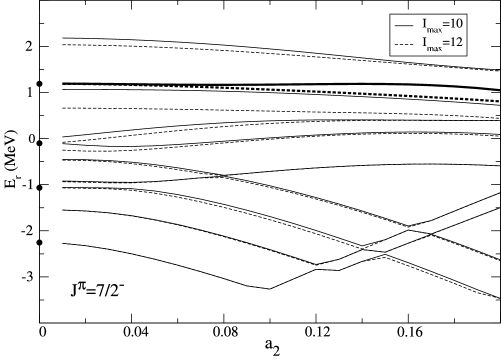
Figure 3: The position of the bound and resonance $J^{\pi}$=7/2^- states in ¹⁴¹Ho calculated in the weak coupling model as a function of the triaxial coupling constant $a_{2}$ for $I_{\rm max}$=10 and 12 ($I_{\rm max}$ is the maximum value of angular momentum considered in the g.s. band and in the gamma band of the daughter nucleus ¹⁴⁰Dy). The results for $I_{\rm max}$=12 are fully converged, i.e., a further increase of the number of states does not change results in the scale of this figure. The axial results without coupling the $\gamma$ band (cf. Table. 1) are marked by the dots. The 7/2^- ground-state of ¹⁴¹Ho is marked by thick lines.

Figure 3 shows that for bound states the convergence is already very satisfactory for $I_{\rm max}$=10; however, this is not true for the 7/2^- band head. For instance, at $a_{2}$=0.1 one obtains for the energy of lowest bound state: -3.254, -3.264, -3.265, -3.265, and -3.265 MeV for $I_{\rm max}$=8, 10, 12, 14, and 16, respectively. In contrast, for the 7/2^- g.s. (marked by thicker lines in Fig. 3) the analogous numbers are: 1.297, 1.171, 1.062, 1.062, and 1.062 MeV. That is, in this case, going from $I_{\rm max}$=10 to $I_{\rm max}$=12 the energy changes by as much as 109 keV. This variation is significant since the width of the resonance is extremely sensitive to its energy. In our previous paper kru03 , we made the pilot studies of the coupling to the $\gamma$ band on proton emission in ¹⁴¹Ho. Unfortunately, in this early analysis based on the coupled-channel method, we took $I_{\rm max}$=10; hence the conclusions of this paper have to be revised (see below).

The width of the 7/2^- band head was computed using the RMHO method assuming $I_{\rm max}$=12. At each value of $a_{2}$ we have adjusted the potential depth so as to get the position of the resonance at 1.19 MeV. The calculated half-life of the resonance and the branching ratio for the decay to the $2^{+}_{1}$ state in ¹⁴⁰Dy are displayed in Figure 4. It is seen that when increasing the coupling to the $\gamma$-band, both the lifetime and the $2^{+}_{1}$ branching ratio increase, and the agreement with experiment gets worse.

Figure 4: Half-life (top) and branching ratio for the decay to the $2^{+}_{1}$ state in ¹⁴⁰Dy (bottom) for the 7/2^- g.s. of ¹⁴¹Ho as a function of the triaxial coupling $a_{2}$. Experimental data ($T_{1/2}$=4 ms and branching ratio 0.7%) are taken from Refs. ryk99 ; Data141Ho . The spectroscopic factor (BCS occupation coefficient) was assumed to be $u^{2}$=0.84 bar00 .

In order to understand the behavior shown in Fig. 4, we analyzed the components of the wave function. Figure 5 shows the weights of various partial waves ($IKlj$) in the 7/2^- g.s. of ¹⁴¹Ho,

$$|C_{IKlj}|^{2}=\int_{0}^{\infty}u^{2}_{IKlj}(r)dr,$$ (45)

as functions of $a_{2}$. According to our calculations, the amplitudes associated with the coupling to the $0^{+}_{1}$ g.s. and $2^{+}_{1}$ state in ¹⁴⁰Dy are fairly small; most of the strength lies in higher-lying states including the channels that are energetically closed for proton emission. The ($0^{+}_{1}$, $f_{7/2}$) amplitude, solely determining the 7/2^-$\rightarrow$$0^{+}_{1}$ decay, gradually decreases with $a_{2}$. Interestingly, while the total $f_{7/2}$ strength increases with $a_{2}$ as expected (the $h_{11/2}$ and $f_{7/2}$ shells are strongly coupled by triaxial field), most of this strength is pushed up to higher-lying states.

Figure 5: Weights (45) of the ($I$=2₁, $l$=5 $j$=11/2), (0₁, 3, 7/2), (2₁, 5, 9/2), and (2₁, 1, 3/2) partial waves of the 7/2^- g.s. of ¹⁴¹Ho as a function of $a_{2}$.

Figure 6 displays partial widths $\Gamma_{c}$ (17) corresponding to various channels of decay to the $0^{+}_{1}$ and $2^{+}_{1}$ states in ¹⁴⁰Dy. The gradual decrease of the (0₁, $f_{7/2}$) partial width (hence the increase of the half-life of ¹⁴¹Ho) with $a_{2}$ can be explained in terms of the (0₁, $f_{7/2}$) amplitude in Fig. 5. The $2^{+}$ branching ratio is almost completely determined by the (2₁, $f_{7/2}$) partial width; the second-order contribution from the $p_{3/2}$ wave is much smaller (cf. inset in Fig. 5).

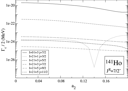
Figure 6: Partial widths $\Gamma_{c}$ (17) corresponding to various $0^{+}_{1}$ and $2^{+}_{1}$ decay channels as functions of $a_{2}$.

V Conclusions

This work contains the first application of the triaxial non-adiabatic weak coupling approach to the description of proton-emitting nuclei. The resulting coupled-channel equations take into account the coupling to the $K$=2 band representing collective $\gamma$ vibrations.

The inclusion of the $\gamma$ band into the weak-coupling formalism increases the number of the coupled channel equations significantly. This makes it very difficult to solve accurately the multitude of coupled differential equations with Gamow boundary condition. In order to overcome this difficulty, we developed a new formalism, dubbed RMHO, which incorporates the variational oscillator expansion method into the R-matrix theory. Within RMHO, it is possible to significantly increase the number of states in the daughter nucleus to guarantee the convergence of the solution.

As an example, the RMHO formalism has been applied to the g.s. proton emission from ¹⁴¹Ho, in which there have been some experimental hints (e.g., large signature splitting in the g.s. rotational band or presence of low-lying $\gamma$-vibrational states in the neighboring even-even nuclei) for triaxiality. Our calculations show that while the coupling to $\gamma$ vibrations can in general influence decay characteristics (half-life, branching ratios), in the case of ¹⁴¹Ho the resulting trend is opposite to what has been observed experimentally. From this point of view, our results support conclusions drawn in the recent work dav03 based on the adiabatic particle-rotor approach. An important piece of physics which is still missing in our non-adiabatic formalism is the inclusion of quasi-particle pairing. We are currently working on incorporating the Hartree-Fock-Bogoliubov couplings Bel87 into our model.

Appendix A Triaxial Coulomb potential

The Coulomb interaction between the proton and the daughter nuclei is

$$V_{C}({\bf r})=\int\frac{\rho({\bf r}^{\prime})}{|{\bf r}-{\bf r}^{\prime}|}d{\bf r}^{\prime},$$ (46)

where the charge density reads

$$\rho({\bf r})=\frac{\rho_{0}}{1+\exp\left[(r-R(\Omega))/a\right]}$$ (47)

and the nuclear surface $R(\Omega)$ is given by Eq. (2). To the first order in $a_{2}$ the Coulomb potential is

$$V_{C}({\bf r})=V^{(1)}_{C}({\bf r})|_{a_{2}=0}+a_{2}V^{(2)}_{C}({\bf r}).$$ (48)

The first term, $V^{(1)}_{C}$, is the Coulomb potential due to an axial symmetric charge density. It is given by a simple expression derived in, e.g., Ref. defcou . The second term, $V^{(2)}_{C}$, is of the form

$$V^{(2)}_{C}({\bf r})=\int\frac{\partial\rho({\bf r}^{\prime})}{\partial a_{2}}\frac{1}{|{\bf r}-{\bf r}^{\prime}|}d{\bf r}^{\prime}.$$ (49)

Calculating the derivative of the charge density and taking the limit of the sharp charge distribution ($a\rightarrow 0$), one obtains

$$V^{(2)}_{C}({\bf r})=R_{0}\rho_{0}C(a_{0},a_{2})\int\frac{R^{2}_{a}(\Omega^{\prime})[Y_{2,2}(\Omega^{\prime})+Y_{2,-2}(\Omega^{\prime})]}{\sqrt{R^{2}_{a}(\Omega^{\prime})+r^{2}-2R_{a}(\Omega^{\prime})r\cos\xi}}d\Omega^{\prime},$$ (50)

where

$$\cos\xi=\cos\theta\cos\theta^{\prime}+\sin\theta\sin\theta^{\prime}\cos(\phi-\phi^{\prime}).$$ (51)

and $R_{a}(\Omega^{\prime})=R(\Omega^{\prime})|_{a_{2}=0}$. This can be reduced to

$$V^{(2)}_{C}({\bf r})=R_{0}\rho_{0}C(a_{0},a_{2})\sqrt{\frac{15}{8\pi}}$$

$$\int_{-1}^{1}dtR^{2}_{a}(t)(1-t^{2})\int_{0}^{2\pi}d\phi^{\prime}\frac{2\cos^{2}\phi^{\prime}-1}{\sqrt{R^{2}_{a}(t)+r^{2}-2R_{a}(t)r\cos\xi}},$$ (52)

where $t=\cos\theta^{\prime}$. The integral over $\phi^{\prime}$ can be calculated analytically, and the final result can be expressed in terms of a simple one-dimensional integral:

$$V^{(2)}_{C}({\bf r})=R_{0}\rho_{0}C(a_{0},a_{2})\sqrt{\frac{15}{8\pi}}\cos({2\phi})$$

$$\int_{-1}^{1}dtR^{2}_{a}(t)(1-t^{2})\frac{4}{3b^{2}\sqrt{a+b}}\left\{(4a^{2}-b^{2})K(\kappa)-4a(a+b)E(\kappa)\right\},$$ (53)

where

$$a=R_{a}^{2}(t)+r^{2}-2R_{a}(t)r\cos\theta\cos\theta^{\prime},$$ (54)

$$b=2R_{a}(t)r\sin\theta\sin\theta^{\prime},$$ (55)

and

$$\kappa=\sqrt{\frac{2b}{a+b}}.$$ (56)

In Eq. (A), $K(\kappa)$ and $E(\kappa)$ are the complete elliptic integral of the first and second kind, respectively.

References

- (1) A.T. Kruppa, B. Barmore, W. Nazarewicz, and T. Vertse, Phys. Rev. Lett. 84, 4549 (2000).
- (2) B. Barmore, A.T. Kruppa, W. Nazarewicz, and T. Vertse, Phys. Rev. C 62, 054315 (2000).
- (3) H. Esbensen and C.N. Davids, Phys. Rev. C 63, 014315 (2001).
- (4) C.N. Davids and H. Esbensen, Phys. Rev. C 64, 034317 (2001).
- (5) K. Hagino, Phys. Rev. C 64, 041304 (2001).
- (6) S.G. Kadmenskiĭ and V.P. Bugrov, Phys. At. Nucl. 59, 399 (1996).
- (7) L.S. Ferreira, E. Maglione, and R.J. Liotta, Phys. Rev. Lett. 78, 1640 (1997).
- (8) E. Maglione, L.S. Ferreira, and R.J. Liotta, Phys. Rev. Lett. 81, 538 (1998).
- (9) C.N. Davids, P.J. Woods, D. Seweryniak, A.A. Sonzogni, J.C. Batchelder, C.R. Bingham, T. Davinson, D.J. Henderson, R.J. Irvine, G.L. Poli, J. Uusitalo, and W.B. Walters, Phys. Rev. Lett. 80, 1849 (1998).
- (10) E. Maglione, L.S. Ferreira, and R.J. Liotta, Phys. Rev. C 59, R589 (1999).
- (11) K. Rykaczewski, J.C. Batchelder, C.R. Bingham, T. Davinson, T.N. Ginter, C.J. Gross, R. Grzywacz, M. Karny, B.D. MacDonald, J.F. Mas, J.W. McConnell, A. Piechaczek, R.C. Slinger, K.S. Toth, W.B. Walters, P.J. Woods, E.F. Zganjar, B. Barmore, L.Gr. Ixaru, A.T. Kruppa, W. Nazarewicz, M. Rizea, and T. Vertse, Phys. Rev. C 60, 011301 (1999).
- (12) A.A. Sonzogni, C.N. Davids, P.J. Woods, D. Seweryniak, M.P. Carpenter, J.J. Ressler, J. Schwartz, J. Uusitalo, and W.B. Walters, Phys. Rev. Lett. 83, 1116 (1999).
- (13) G. Fiorin, E. Maglione, and L.S. Ferreira, Phys. Rev. C 67, 054302 (2003).
- (14) A. Bohr and B.R. Mottelson, Nuclear Structure Vol. II, Benjamin, New York, 1975.
- (15) C.N. Davids and H. Esbensen, Proton-Emitting Nuclei Second International Symposium PROCON 2003, Eds. E. Maglione and F. Soramel, AIP Conference Proceedings, Volume 681, p. 41, Melville, New York, 2003.
- (16) A.T. Kruppa and W. Nazarewicz, Proton-Emitting Nuclei Second International Symposium PROCON 2003, Eds. E. Maglione and F. Soramel, AIP Conference Proceedings, Volume 681, p. 61, Melville, New York, 2003.
- (17) D. Seweryniak, P.J. Woods, J.J. Ressler, C.N. Davids, A. Heinz, A.A. Sonzogni, J. Uusitalo, W.B. Walters, J.A. Caggiano, M.P. Carpenter, J.A. Cizewski, T. Davinson, K.Y. Ding, N. Fotiades, U. Garg, R.V.F. Janssens, T.L. Khoo, F.G. Kondev, T. Lauritsen, C.J. Lister, P. Reiter, J. Shergur, and I. Wiedenhöver, Phys. Rev. Lett. 86, 1458 (2001).
- (18) Evaluated Nuclear Structure Data File, http://www.nndc.bnl.gov/nndc/ensdf.
- (19) W.B. Walters, private communication, 2001.
- (20) J. Yan, P. von Brentano, and A. Gelberg, Phys. Rev. C 48, 1046 (1993).
- (21) M.O. Kortelahti, B.D. Kern, R.A. Braga, R.W. Fink, I.C. Girit, and R.L. Mlekodaj, Phys. Rev. C 42, 1267 (1990).
- (22) C.N. Davids and H. Esbensen, arXiv:nucl-th/0311034.
- (23) W. Królas, R. Grzywacz, K.P. Rykaczewski, J.C. Batchelder, C.R. Bingham, C.J. Gross, D. Fong, J.H. Hamilton, D.J. Hartley, J.K. Hwang, Y. Larochelle, T.A. Lewis, K.H. Maier, J.W. McConnell, A. Piechaczek, A.V. Ramayya, K. Rykaczewski, D. Shapira, M.N. Tantawy, J.A. Winger, C.-H. Yu, E.F. Zganjar, A.T. Kruppa, W. Nazarewicz, and T.Vertse Phys. Rev. C 65, 031303(R) (2002).
- (24) D.M. Cullen, M.P. Carpenter, C.N. Davids, A.M. Fletcher, S.J. Freeman, R.V.F. Janssens, F.G. Kondev, C.J. Lister, L.K. Pattison, D. Seweryniak, J.F. Smith, A.M. Bruce, K. Abu Saleem, I. Ahmad, A. Heinz, T.L. Khoo, E.F. Moore, G. Mukherjee, C. Wheldon, and A. Woehr, Phys. Lett. 529B, 42 (2002).
- (25) T. Berggren, Nucl. Phys. A109, 265 (1968).
- (26) T. Vertse, P. Curutchet, and R.J. Liotta, Lecture Notes in Physics 325 (Springer Verlag, Berlin 1987), p. 179.
- (27) N. Michel, W. Nazarewicz, M. Płoszajczak, and K. Bennaceur, Phys. Rev. Lett. 89, 042502 (2002).
- (28) N.Michel, W. Nazarewicz, M. Płoszajczak, and J. Okołowicz, Phys. Rev. C 67, 054311 (2003).
- (29) R. Id. Betan, R.J. Liotta, N. Sandulescu, and T. Vertse, Phys. Rev. Lett. 89, 042501 (2002).
- (30) A.U. Hazi, and H.S. Taylor, Phys. Rev. A 1, 1109 (1970).
- (31) W.P. Reinhardt, Comput. Phys. Commun. 17, 1 (1979).
- (32) R.G. Lovas and M.A. Nagarajan, J. Phys. A 15, 2383 (1982).
- (33) V.A. Mandelshtam, T.R. Ravuri, and H.S. Taylor, Phys. Rev. Lett. 70, 1932 (1993).
- (34) R. Salzgeber, U. Manthe, Th. Weiss, and Ch. Schlier, Chem. Phys. Lett. 249, 237 (1996).
- (35) A.T. Kruppa and K. Arai, Phys. Rev. A 59, 3556 (1999).
- (36) K. Arai and A.T. Kruppa, Phys. Rev. C 60, 064315 (1999).
- (37) A.T. Kruppa, W. Nazarewicz, and P.B. Semmes, Proc. Int. Symposium on Proton-Emitting Nuclei, ed. by J.C. Batchelder, AIP Conference Proceedings 518 (American Institute of Physics, New York, 2000), p. 173.
- (38) T. Tamura, Rev. Mod. Phys. 37, 679 (1965).
- (39) T. Tamura, Nucl. Phys. 73, 241 (1965)
- (40) J. Humblet and L. Rosenfeld, Nucl. Phys. 26, 529 (1961).
- (41) A. M. Lane and R. G. Thomas, Rev. Mod. Phys 30, 257 (1958).
- (42) R.G. Thomas, Prog. Theor. Phys. 12, 253 (1954).
- (43) K.P. Rykaczewski, R.K. Grzywacz, J.C. Batchelder, C.R. Bingham, C.J. Gross, D. Fong, J.H. Hamilton, D.J. Hartley, P. Hausladen, J.K. Hwang, M. Karny, W. Królas, Y. Larochelle, T.A. Lewis, K.H. Maier, J.W. McConnell, A. Piechaczek, A.V. Ramayya, K. Rykaczewski, D. Shapira, M.N. Tantawy, J.A. Winger, C.-H. Yu, E.F. Zganjar, A.T. Kruppa, W. Nazarewicz, T. Vertse, and K. Hagino, Proceedings of Int. Conf. on Nuclear Structure Mapping the Triangle, Grand Teton National Park, Wyoming, May 22-25, 2002, ed. by A. Aprahamian, J.A. Cizewski, S. Pittel, N.V. Zamfir (AIP Proceedings, No. 638; Melville, New York 2002), p. 149
- (44) S.T. Belyaev, A.V. Smirnov, S.V. Tolokonnikov, and S.A. Fayans, Sov. J. Nucl. Phys. 45, 783 (1987).
- (45) M. Brack, J. Damgård, A.S. Jensen, H.C. Pauli, V.M. Strutinsky and C. Y. Wong, Rev. Mod. Phys. 44, 320 (1972).