Large-angle scattering and quasi-elastic barrier distributions

Abstract

We study in detail the barrier distributions extracted from large-angle quasi-elastic scattering of heavy ions at energies near the Coulomb barrier. Using a closed-form expression for scattering from a single barrier, we compare the quasi-elastic barrier distribution with the corresponding test function for fusion. We examine the isocentrifugal approximation in coupled-channels calculations of quasi-elastic scattering and find that for backward angles, it works well, justifying the concept of a barrier distribution for scattering processes. This method offers an interesting tool for investigating unstable nuclei. We illustrate this for the ³²Mg + ²⁰⁸Pb reaction, where the quadrupole collectivity of the neutron-rich ³²Mg remains to be clarified experimentally.

I Introduction

Heavy-ion collisions at energies around the Coulomb barrier provide an ideal opportunity to study quantum tunneling phenomena in systems with many degrees of freedom [1, 2]. In a simple model, a potential barrier for the relative motion between the colliding nuclei is created by the strong interplay of the repulsive Coulomb force with the attractive nuclear interaction. In the eigenchannel approximation, this barrier is split into a number of distributed barriers due to couplings of the relative motion to intrinsic degrees of freedom (such as collective inelastic excitations of the colliding nuclei and/or transfer processes), resulting in the subbarrier enhancement of fusion cross sections [3]. It is now well known that a barrier distribution can be extracted experimentally from the fusion excitation function $\sigma_{\rm fus}(E)$ by taking the second derivative of the product $E\sigma_{\rm fus}(E)$ with respect to the center-of-mass energy $E$, that is, $d^{2}(E\sigma_{\rm fus})/dE^{2}$. This method was first proposed by Rowley, Satchler, and Stelson in Ref. [4], and has stimulated precise measurements of fusion cross sections for many systems [5, 6] (see Ref. [1] for a detailed review). The extracted fusion barrier distributions have been found to be very sensitive to the structure of the colliding nuclei, and thus the barrier distribution method has opened up the possibility of using the heavy-ion fusion reaction as a “quantum tunneling microscope” in order to investigate both the static and dynamical properties of atomic nuclei.

Channel couplings also affect the scattering process. In Ref. [7], it was suggested that the same information as the fusion cross section may be obtained from the cross section for quasi-elastic scattering (a sum of elastic, inelastic, and transfer cross sections) at large angles. At these backward angles, it is known that the single-barrier elastic cross section falls off smoothly from a value close to that for Rutherford scattering at low energies to very small values at energies high above the barrier. Timmers et al. therefore proposed to use the first derivative of the ratio of the quasi-elastic cross section $\sigma_{\rm qel}$ to the Rutherford cross section $\sigma_{R}$ with respect to energy, $-d(d\sigma_{\rm qel}/d\sigma_{R})/dE$, as an alternative representation of the barrier distribution [8]. The experimental data of Timmers et al. have revealed [8] that the quasi-elastic barrier distribution is indeed similar to that for fusion, although the former may be somewhat smeared and thus less sensitive to nuclear structure effects.

There are certain attractive experimental advantages to measuring the quasi-elastic cross section $\sigma_{\rm qel}$ rather than the fusion cross sections $\sigma_{\rm fus}$ to extract a representation of the barrier distribution[9]. These are: i) less accuracy is required in the data for taking the first derivative rather than the second derivative, ii) whereas measuring the fusion cross section requires specialized recoil separators (electrostatic deflector/velocity filter) usually of low acceptance and efficiency, the measurement of $\sigma_{\rm qel}$ needs only very simple charged-particle detectors, not necessarily possessing good resolution either in energy or in charge, and iii) several effective energies can be measured at a single-beam energy, since, in the semi-classical approximation, each scattering angle corresponds to scattering at a certain angular momentum, and the cross section can be scaled in energy by taking into account the centrifugal correction. The last point not only improves the efficiency of the experiment, but also allows the use of a cyclotron accelerator where the relatively small energy steps required for barrier distribution experiments cannot be obtained from the machine itself. This fact was recently exploited by Piasecki et al.[10], who took an astute choice of the scattering angles at which $\sigma_{\rm qel}$ was measured in order to have the energy range necessary, while retaining relatively small energy steps. Moreover, these advantages all point to greater ease of measurement with low-intensity exotic beams.

In this paper, we undertake a detailed discussion of the properties of the quasi-elastic barrier distribution. In contrast to the fusion barrier distribution, a theoretical description of the quasi-elastic barrier distribution has been limited so far either to a purely classical level or to a completely numerical level. Given that many new barrier distribution measurements for exotic nuclei are expected to come out in the near future, due to an increasing availability of radioactive beams, we believe that it is of considerable importance to clarify the properties of the quasi-elastic barrier distribution in a more reliable and transparent way.

The paper is organized as follows. In Sec. II, we consider a single-barrier system and discuss test functions for the barrier distribution, that is the representations of the barrier distribution for a single barrier case. We first briefly review the fusion test function, and discuss the relation to the barrier penetrability. We then use semi-classical perturbation theory [11, 12] to derive an analytical expression for the elastic cross section at backward angles. Using the formula thus obtained, we discuss the energy dependence of the quasi-elastic test function, and compare it with that for the fusion test function. We also discuss the scaling property of the quasi-elastic test function obtained at different scattering angles. In Sec. III, we discuss the barrier distribution for coupled-channels systems. Theoretically, barrier distributions have a clear physical meaning only in the limit of zero angular momentum transfer (that is, in the isocentrifugal approximation [13, 14, 15, 16, 17, 18, 19, 20, 21]) with vanishing excitation energies for the intrinsic degrees of freedom. In this limit the barrier distribution representation may be derived analytically as a weighted sum of test functions. Nevertheless, a simple two-level model suggests that the concept holds to a good approximation even when the excitation energy is finite [22]. And of course many experimental data also show well-defined barrier structures, which can be reproduced by coupled-channels calculations, even for systems where the excitation energies are large. However, although the validity of the isocentrifugal approximation has been shown to work well for fusion [18], its applicability for scattering processes in the presence of the long-range Coulomb interaction is less clear [17, 19, 20, 21]. We therefore re-examine its validity for the quasi-elastic barrier distribution. In Sec. IV, we consider the quasi-elastic barrier distribution as applied to reactions induced by exotic nuclei. In particular, we demonstrate its usefulness by showing the possible effects of the quadrupole excitation of ³²Mg in the ³²Mg + ²⁰⁸Pb system. We summarize the paper in Sec. V.

II Single-barrier problems

In this section, we discuss heavy-ion reactions between inert nuclei. For such a system, the incident flux of the projectile is either absorbed or elastically scattered from the target nucleus. We use a local optical potential which is energy and angular momentum independent. Assuming that the imaginary part of the optical potential is strong enough and is localized well inside the Coulomb barrier, the absorption cross section is identified with the fusion cross section.

A Fusion test function

Let us first discuss the properties of the fusion test function. The classical fusion cross section is given by,

$$\sigma^{cl}_{\rm fus}(E)=\pi R_{b}^{2}\left(1-\frac{B}{E}\right)\,\theta(E-B),$$ (1)

where $R_{b}$ and $B$ are the barrier position and the barrier height, respectively. From this expression, it is clear that the first derivative of $E\sigma^{cl}_{\rm fus}$ is proportional to the classical penetrability for a 1-dimensional barrier of height $B$ or eqivalently the s-wave penetrability,

$$\frac{d}{dE}[E\sigma^{cl}_{\rm fus}(E)]=\pi R_{b}^{2}\,\theta(E-B)=\pi R_{b}^{2}\,P_{cl}(E),$$ (2)

and the second derivative to a delta function,

$$\frac{d^{2}}{dE^{2}}[E\sigma^{cl}_{\rm fus}(E)]=\pi R_{b}^{2}\,\delta(E-B).$$ (3)

In quantum mechanics, the tunneling effect smears the delta function in Eq. (3). An analytic formula for the fusion cross section can be obtained if one approximates the Coulomb barrier as an inverse parabola, and is given by [23],

$$\sigma_{\rm fus}(E)=\frac{\hbar\Omega}{2E}R_{b}^{2}\ln\left[1+e^{2\pi(E-B)/\hbar\Omega}\right],$$ (4)

where $\hbar\Omega$ is the curvature of the Coulomb barrier. Again, the first derivative of $E\sigma_{\rm fus}$ is proportional to the s-wave penetrability for a parabolic barrier,

$$\frac{d}{dE}[E\sigma_{\rm fus}(E)]=\pi R_{b}^{2}\,\frac{1}{1+\exp\left[-\frac{2\pi}{\hbar\Omega}(E-B)\right]}=\pi R_{b}^{2}\,P(E).$$ (5)

Defining the function $G_{\rm fus}(E)$ as,

$$G_{\rm fus}(E)\equiv\frac{1}{\pi R_{b}^{2}}\,\frac{d^{2}}{dE^{2}}[E\sigma_{\rm fus}(E)],$$ (6)

eq. (5) leads to

$$G_{\rm fus}(E)=\frac{dP(E)}{dE}=\frac{2\pi}{\hbar\Omega}\,\frac{e^{x}}{(1+e^{x})^{2}},$$ (7)

where $x\equiv 2\pi(E-B)/\hbar\Omega$. This function has the following properties: i) it is symmetric around $E=B$, ii) it is centered on $E=B$, iii) its integral over $E$ is unity, and iv) it has a relatively narrow width of around $\hbar\Omega\ln(3+\sqrt{8})/\pi\sim 0.56\hbar\Omega$. In the next section, we will show that a barrier distribution can be expressed as a weighted sum of normalized functions $G(E)$ (see Eq. (22)). The function $G_{\rm fus}(E)$, therefore, plays the role of a test function, and we call it the fusion test function.

B Quasi-elastic test function

We now ask ourselves the question of how best to define a similar test function for a scattering problem. In the pure classical approach, in the limit of a strong Coulomb field, the differential cross sections for elastic scattering at $\theta=\pi$ is given by,

$$\sigma_{\rm el}^{cl}(E,\pi)=\sigma_{R}(E,\pi)\,\theta(B-E),$$ (8)

where $\sigma_{R}(E,\pi)$ is the Rutherford cross section. Thus, the ratio $\sigma_{\rm el}^{cl}(E,\pi)/\sigma_{R}(E,\pi)$ is the classical reflection probability $R(E)$ ($=1-P(E)$), and Eq. (7) suggests that the appropriate test function for scattering is [8],

$$G_{\rm qel}(E)=-\frac{dR(E)}{dE}=-\frac{d}{dE}\left(\frac{\sigma_{\rm el}(E,\pi)}{\sigma_{R}(E,\pi)}\right).$$ (9)

In realistic systems, however, due to the effect of nuclear distortion, the differential cross section deviates from the Rutherford cross section even at energies below the barrier. Using the semi-classical perturbation theory [11, 12, 24], we derive in the Appendix a semi-classical formula for the backward scattering which takes into account the nuclear effect to the leading order. The result for a scattering angle $\theta$ reads,

$$\frac{\sigma_{\rm el}(E,\theta)}{\sigma_{R}(E,\theta)}=\alpha(E,\lambda_{c})\cdot|S(E,\lambda_{c})|^{2},$$ (10)

where $S(E,\lambda_{c})$ is the total (Coulomb + nuclear) $S$-matrix at energy $E$ and angular momentum $\lambda_{c}=\eta\cot(\theta/2)$, with $\eta$ being the usual Sommerfeld parameter. Note that $|S(E,\lambda_{c})|^{2}$ is nothing but the reflection probability of the Coulomb barrier. For $\theta=\pi$, $\lambda_{c}$ is zero, and $|S(E,\lambda_{c}=0)|^{2}$ is given by

$$|S(E,\lambda_{c}=0)|^{2}=R(E)=\frac{\exp\left[-\frac{2\pi}{\hbar\Omega}(E-B)\right]}{1+\exp\left[-\frac{2\pi}{\hbar\Omega}(E-B)\right]}$$ (11)

in the parabolic approximation. $\alpha(E,\lambda_{c})$ in Eq. (10) is given by

$$\alpha(E,\lambda_{c})=1+\frac{V_{N}(r_{c})}{ka}\,\frac{\sqrt{2a\pi k\eta}}{E}\,\left[1-\frac{r_{c}}{Z_{P}Z_{T}e^{2}}\cdot 2V_{N}(r_{c})\left(\frac{r_{c}}{a}-1\right)\right],$$ (12)

where $k=\sqrt{2\mu E/\hbar^{2}}$, with $\mu$ being the reduced mass for the colliding system. The nuclear potential $V_{N}(r_{c})$ is evaluated at the Coulomb turning point $r_{c}=(\eta+\sqrt{\eta^{2}+\lambda_{c}^{2}})/k$, and $a$ is the diffuseness parameter in the nuclear potential.

The upper panel of Fig. 1 shows the excitation function of the cross sections at $\theta=\pi$ for the ¹⁶O + ¹⁴⁴Sm reaction. We use an optical potential of the Woods-Saxon form, with parameters $V_{0}$ = 105.1 MeV, $r_{0}$ = 1.1 fm, $a$ = 0.75 fm, $W$=30 MeV, $r_{W}$ = 1.0 fm, and $a_{W}$ = 0.4 fm. The solid line is the exact solution of the Schrödinger equation, while the dashed line is obtained with the semi-classical formula (10). The dotted line shows the reflection probability $R(E)=|S(E)|^{2}$. We clearly see that the semi-classical formula accounts well for the deviation of the elastic cross section $\sigma_{\rm el}(E)$ from the Rutherford cross section around the Coulomb barrier.

The corresponding quasi-elastic test functions, $G_{\rm qel}(E)=-d/dE(\sigma_{\rm el}/\sigma_{R})$, are shown in the lower panel of Fig. 1. We use a point-difference formula with $\Delta E_{\rm cm}=1.8$ MeV (as in an experiment) in order to evaluate the energy derivative. Notice that the first derivative of the reflection probability (dotted line) corresponds to the fusion test function $G_{\rm fus}(E)$ given in Eq. (7). Because of the nuclear distortion factor $\alpha(E,\lambda_{c})$, the quasi-elastic test function behaves a little less simply than that for fusion. We find: i) the peak position slightly deviates from the barrier height $B$ (by 0.265 MeV for the example shown in Fig. 1), and ii) it has a low-energy tail. Eq. (10) indicates that there are two contributions to the quasi-elastic test function. One is $\alpha(E)\cdot dR(E)/dE$, and the other $d\alpha(E)/dE\cdot R(E)$. In Fig.2, we show these two contributions separately. We notice that the low-energy tail of the quasi-elastic test function comes from the latter, that is, the energy dependence of the nuclear distortion factor $\alpha(E)$.

Despite these small drawbacks, the quasi-elastic test function $G_{\rm qel}(E)$ behaves rather similarly to the fusion test function $G_{\rm fus}(E)$. In particular, both functions have a similar, relatively narrow, width, and their integral over $E$ is unity. We may thus consider that the quasi-elastic test function is an excellent analogue of the one for fusion, and we exploit this fact in studying barrier structures in heavy-ion scattering.

Notwithstanding the above comments, it is clear that the quasi-elastic test function defined above depends on the scattering angle, and below we shall show how the test function can be scaled in terms of an effective energy.

C Scaling property of the quasi-elastic test function

One of the advantages of the quasi-elastic test function over the fusion test function is that different scattering angles correspond to the different grazing angular momenta. To some extent, the effect of angular momentum can be corrected by shifting the energy by an amount equal to the centrifugal potential. Estimating the centrifugal potential at the Coulomb turning point $r_{c}$, the effective energy may be expressed as [8]

$$E_{\rm eff}\sim E-\frac{\lambda_{c}^{2}\hbar^{2}}{2\mu r_{c}^{2}}=2E\frac{\sin(\theta/2)}{1+\sin(\theta/2)}.$$ (13)

In deriving this equation, we have used the definition of $r_{c}$, that is, $E=Z_{P}Z_{T}e^{2}/r_{c}+\lambda_{c}^{2}\hbar^{2}/2\mu r_{c}^{2}$. Therefore, one expects that the function $-d/dE(\sigma_{\rm el}/\sigma_{R})$ evaluated at an angle $\theta$ will correspond to the quasi-elastic test function (9) at the effective energy given by eq. (13).

In order to check the scaling property of the quasi-elastic test function with respect to the angular momentum, Fig. 3 compares the functions $\sigma_{\rm el}/\sigma_{R}$ (upper panel) and $-d/dE(\sigma_{\rm el}/\sigma_{R})$ (lower panel) obtained at two different scattering angles. The solid line is evaluated at $\theta=\pi$, while the dotted line at $\theta=160^{\rm o}$. The dashed line is the same as the dotted line, but shifted in energy by $E_{\rm eff}-E$. Evidently, the scaling does work well, both at energies below and above the Coulomb barrier.

We should note, however, that as the scattering angle decreases, the scaling becomes less good. See Fig. 4 for the scaling property for $\theta=140^{\rm o}$. Thus in planning an experiment (especially if it combines data taken in detectors at different angles), one should take careful account of this effect. Also at smaller angles, it is well known that the underlying elastic cross section will display Fresnel oscillations, which would cause the test function itself (and any derived distribution) to oscillate. Detector angles are best chosen to minimise effects of Fresnel oscillations.

III Barrier distribution for multi-channel systems

A Barrier distributions in the sudden tunneling limit

Let us now discuss the barrier distributions in the presence of a coupling between the relative motion $r$ and an intrinsic degree of freedom $\xi$. The standard way to address the effect of the coupling is to solve the coupled-channels equations. For a problem of heavy-ion fusion reactions, these equations are often solved in the iso-centrifugal approximation [25], where one replaces the angular momentum of the relative motion in each channel by the total angular momentum $J$ (this approximation is also referred to as the rotating frame approximation or the no-Coriolis approximation in the literature). The iso-centrifugal approximation dramatically simplifies the angular momentum couplings, and reduces the dimension of the coupled-channels equations in a considerable way [13, 14, 15, 16, 17, 18, 19, 20, 21]. The coupled-channels equations in this approximation are given by

$$\left(-\frac{\hbar^{2}}{2\mu}\frac{d^{2}}{dr^{2}}+\frac{J(J+1)\hbar^{2}}{2\mu r^{2}}+V_{0}(r)-E+\epsilon_{I}\right)u_{I}(r)$$ (14)

$$+\sum_{I^{\prime}}\sqrt{\frac{2\lambda+1}{4\pi}}f(r)\langle\varphi_{I0}|T_{\lambda 0}|\varphi_{I^{\prime}0}\rangle u_{I^{\prime}}(r) = 0,$$ (15)

where $|\varphi_{IM}\rangle$ is an intrinsic wave function which satisfies $H_{\rm int}|\varphi_{IM}\rangle=\epsilon_{I}|\varphi_{IM}\rangle$. We have assumed that the coupling Hamiltonian is given by $V_{\rm coup}=f(r)Y_{\lambda\mu}(\hat{\mbox{\boldmath$r$}})\hat{T}^{*}_{\lambda\mu}(\xi)$. The coupled-channels equations are solved with the scattering boundary condition for $u_{I}(r)$,

$$u_{I}(r)\to\frac{i}{2}\left\{H_{J}^{(-)}(k_{i}r)\delta_{I,I_{i}}-\sqrt{\frac{k_{i}}{k_{I}}}S^{J}_{I}H_{J}^{(+)}(k_{I}r)\right\},$$ (16)

where $S^{J}_{I}$ is the nuclear S-matrix. $H_{l}^{(-)}(kr)$ and $H_{l}^{(+)}(kr)$ are the incoming and the outgoing Coulomb wave functions, respectively. The channel wave number $k_{I}$ is given by $\sqrt{2\mu(E-\epsilon_{I})/\hbar^{2}}$, and $k_{i}=k_{I_{i}}=\sqrt{2\mu E/\hbar^{2}}$. The scattering angular distribution for the channel $I$ is then given by [17],

$$\frac{d\sigma_{I}}{d\Omega}=\frac{k_{I}}{k_{i}}|f_{I}(\theta)|^{2},$$ (17)

with

$$f_{I}(\theta)=\sum_{J}e^{i[\sigma_{J}(E)+\sigma_{J}(E-\epsilon_{I})]}\sqrt{\frac{2J+1}{4\pi}}\,Y_{J0}(\theta)\,\frac{-2i\pi}{\sqrt{k_{i}k_{lI}}}(S^{J}_{I}-\delta_{I,I_{i}})+f_{C}(\theta)\delta_{I,I_{i}},$$ (18)

where $\sigma_{J}(E)$ and $f_{C}(\theta)$ are the Coulomb phase shift and the Coulomb scattering amplitude, respectively.

In the limit of $\epsilon_{I}\to 0$, the reduced coupled-channels equations (15) are completely decoupled. In this limit, the coupling matrix defined as

$$V_{II^{\prime}}\equiv\epsilon_{I}\delta_{I,I^{\prime}}+\sqrt{\frac{2\lambda+1}{4\pi}}f(r)\langle\varphi_{I0}|T_{\lambda 0}|\varphi_{I^{\prime}0}\rangle$$ (19)

can be diagonalized independently of $r$. It is then easy to prove that the fusion and the quasi-elastic cross sections are given as a weighted sum of the cross sections for uncoupled eigenchannels[14, 15],

$$\sigma_{\rm fus}(E) = \sum_{\alpha}w_{\alpha}\sigma_{\rm fus}^{(\alpha)}(E),$$ (20)

$$\sigma_{\rm qel}(E,\theta) = \sum_{I}\sigma_{I}(E)=\sum_{\alpha}w_{\alpha}\sigma_{\rm el}^{(\alpha)}(E,\theta),$$ (21)

where $\sigma_{\rm fus}^{(\alpha)}(E)$ and $\sigma_{\rm el}^{(\alpha)}(E,\theta)$ are the fusion and the elastic cross sections for a potential in the eigenchannel $\alpha$, that is, $V_{\alpha}(r)=V_{0}(r)+\lambda_{\alpha}(r)$. Here, $\lambda_{\alpha}(r)$ is the eigenvalue of the coupling matrix (19) (when $\epsilon_{I}$ is zero, $\lambda_{\alpha}(r)$ is simply given by $\lambda_{\alpha}\cdot f(r)$). The weight factor $w_{\alpha}$ is given by $w_{\alpha}=U_{0\alpha}^{2}$, where $U$ is the unitary matrix which diagonalizes Eq. (19). Eqs. (20) and (21) immediately lead to the expressions for the barrier distribution in terms of the test functions introduced in the previous section,

$$D_{\rm fus}(E) = \frac{d^{2}}{dE^{2}}[E\sigma_{\rm fus}(E)]=\sum_{\alpha}w_{\alpha}\pi R_{b,\alpha}^{2}\,G_{\rm fus}^{(\alpha)}(E),$$ (22)

$$D_{\rm qel}(E) = -\frac{d}{dE}\left(\frac{\sigma_{\rm qel}(E,\pi)}{\sigma_{R}(E,\pi)}\right)=\sum_{\alpha}w_{\alpha}G_{\rm qel}^{(\alpha)}(E).$$ (23)

As an example of these formulas, let us consider the effect of rotational excitations of the target nucleus in the reaction of ¹⁶O with the deformed ¹⁵⁴Sm. For this problem, cross sections (20) and (21) can be computed as [26]

$$\sigma(E)=\int^{1}_{0}d(\cos\theta_{T})\sigma(E;\theta_{T}),$$ (24)

where $\theta_{T}$ is the orientation of the deformed target. The angle dependent potential $V(r,\theta_{T})$ is given by,

$$V(r,\theta_{T}) = V_{N}(r,\theta_{T})+V_{C}(r,\theta_{T}),$$ (25)

$$V_{N}(r,\theta_{T}) = \frac{-V_{0}}{1+\exp[(r-R-R_{T}\beta_{2}Y_{20}(\theta_{T})-R_{T}\beta_{4}Y_{40}(\theta_{T}))]},$$ (26)

$$V_{C}(r,\theta_{T}) = \frac{Z_{P}Z_{T}e^{2}}{r}+\sum_{\lambda}\left(\beta_{\lambda}+\frac{2}{7}\sqrt{\frac{5}{\pi}}\beta_{2}^{2}\delta_{\lambda,2}\right)\,\frac{3Z_{P}Z_{T}e^{2}}{2\lambda+1}\frac{R_{T}^{\lambda}}{r^{\lambda+1}}Y_{\lambda 0}(\theta_{T}).$$ (27)

Figs. 5(a) and 5(b) show the barrier distributions obtained with Eq. (24) for the fusion and the quasi-elastic processes, respectively. We use the potential whose parameters are $V_{0}$=220 MeV, $R=1.1\times(A_{T}^{1/3}+A_{P}^{1/3})$ fm, and $a$=0.65 fm. The deformation parameters are taken to be $\beta_{2}$=0.306 and $\beta_{4}$=0.05. We replace the integral in Eq. (24) with the $(I_{\rm max}+2)$-point Gauss quadrature [15] with $I_{\rm max}$=10. That is, we take 6 different orientation angles. The contributions from each eigenbarrier are shown by the dashed line in Fig. 5(a) and Fig. 5(b). The solid line is the sum of all the contributions, which is compared with the experimental data [5, 8]. The agreement between the calculation and the experimental data is reasonable both for the fusion and the quasi-elastic barrier distributions. For the fusion barrier distribution $D_{\rm fus}$, the agreement will be further improved if one uses a larger value of diffuseness parameter $a$ [5, 27] (see the dotted line). Fig. 5(c) compares the fusion with the quasi-elastic barrier distributions. These are normalized so that the energy integral between 50 and 70 MeV is unity. As we discussed in Sec. II for a single barrier case, we see that the two barrier distributions show a very similar behavior to each other.

B Barrier distributions in systems with finite excitation energy

In general, the approximation of neglecting the excitation energies $\epsilon_{I}$ (that is, the sudden tunneling approximation) is valid only for rotational states in heavy deformed nuclei. Despite this, however, some of the most interesting effects have been found in the fusion barrier distributions for systems involved with highly vibrational nuclei as well [5, 6]. One finds that the barrier structures still exist, but that the weights of the different barriers can be strongly influenced by non-adiabatic effects. In Ref. [22], we have explicitly demonstrated that the fusion cross sections are in general given by Eq. (20), but with the energy dependent weight factors $w_{\alpha}(E)$ (in the sudden tunneling limit, the weight factors become energy independent). For a simple two-channel problem, we found that although the weights may depend strongly on the excitation energy, their dependence on the incident energy is weak, suggesting that the concept of a barrier distribution holds good even for finite intrinsic excitation energies [22]. Since the quasi-elastic barrier distribution $G_{\rm qel}(E)$ is related to the fusion barrier distribution $G_{\rm fus}(E)$ through flux conservation (unitarity), a similar situation can be expected for the quasi-elastic barrier distribution.

C Applicability of the iso-centrifugal approximation

As we have mentioned in Sec. I, the validity of the iso-centrifugal approximation has been well tested for heavy-ion fusion reactions[18]. In contrast, it is known that the approximation fails to reproduce the exact result for scattering angular distributions in the presence of the long-range Coulomb force. The effect of the coupling is somewhat overestimated in the isocentrifugal approximation, and simple recipes to renormalize the coupling strength have been proposed in order to cure this problem [17, 19, 20, 21]. On the other hand, Esbensen et al. have argued, based on semi-classical considerations, that the isocentrifugal approximation (without renormalization of the coupling strength) works better for backward angle scattering [17].

Since it has not yet been clear how well the isocentrifugal approximation works in connection with the quasi-elastic barrier distribution, we re-examine in this subsection the performance of the approximation for large-angle scattering. To this end, we consider the effect of quadrupole phonon excitations in the target nucleus for the ¹⁶O + ¹⁴⁴Sm reaction. In order to emphasise the coupling effect, we increase the coupling strength and reduce the excitation energy from the physical values. The values which we use are: $\beta_{2}$=0.2 (with $r_{\rm coup}$ = 1.06 fm) and $\epsilon_{2}$=0.5 MeV. We have checked that our conclusions are not altered irrespective of the values of $\beta_{2}$ and $\epsilon_{2}$. For simplicity, we consider only a single phonon excitation, and employ the linear coupling approximation [28]. We use the same optical potential as in Sec. II.

Figure 6 shows the partial cross sections at $E_{\rm cm}$=65 MeV for the angle-integrated inelastic scattering (upper panel) and for the fusion reaction (lower panel) as a function of the initial orbital angular momentum $l_{i}=J$. The solid line is the exact result of the coupled-channels equations with the full angular momentum couplings, while the dashed line is obtained with the iso-centrifugal approximation. We find that the isocentrifugal approximation works rather well for $J\leq 20$, although the agreement is poor for larger values of $J$. For fusion, only small values of $J$ contribute, and the isocentrifugal approximation always makes an excellent approximation. Fig. 7 shows the angular distributions for the elastic (upper panel) and inelastic scattering (lower panel). Although the isocentrifugal approximation does not reproduce the main structure of the angular distribution, it indeed works very nicely at backward angles where the main contribution comes from small values of angular momentum (see Eq. (10) and Fig. 6). In fact, the isocentrifugal approximation almost reproduces the exact result for the scattering angles $\theta_{cm}>130^{\rm o}$.

Fig. 8 shows the excitation function for quasi-elastic scattering (upper panel) and its energy derivative calculated at $\theta=170^{\rm o}$ in the laboratory frame. One sees that the isocentrifugal approximation well reproduces the exact solution. We thus conclude that the the isocentrifugal approximation works sufficiently well for studies of quasi-elastic barrier distributions. This fact not only makes the coupled-channels calculations considerably easier, but also assures the similarity of fusion and quasi-elastic distributions even in the presence of channel couplings.

IV Quasi-elastic scattering with radioactive beams

It has been well recognized that low-energy reactions provide an ideal tool to probe the detailed structure of atomic nuclei. The heavy-ion fusion reaction around the Coulomb barrier is one of the typical examples. In the last decade, many high-precision measurements of fusion cross sections have been made, and the nuclear structure information has been successfully extracted through the representation of the fusion barrier distribution [1].

Low-energy radioactive beams have also become increasingly available in recent years, and heavy-ion fusion reactions involving neutron-rich nuclei have been performed for a few systems [29, 30, 31, 32, 33]. New generation facilities have been under construction at several laboratories, and many more reaction measurements with exotic beams at low energies will be performed in the near future (see Ref. [34] for a recent theoretical review). Although it would still be difficult to perform high-precision measurements of fusion cross sections with radioactive beams, the measurement of the quasi-elastic barrier distribution, which can be obtained much more easily than the fusion counterpart as we mentioned in the introduction, may be feasible. Since the quasi-elastic barrier distribution contains similar information as the fusion barrier distribution, the quasi-elastic measurements at backward angles may open up a novel way to probe the structure of exotic neutron-rich nuclei.

In order to demonstrate the usefulness of the study of the quasi-elastic barrier distribution with radioactive beams, we take as an example the reaction ³²Mg and ²⁰⁸Pb. The neutron-rich ³²Mg nucleus has attracted much interest as evidence for the breaking of the $N$=20 spherical shell closure. In this nucleus, a large $B(E2)$ value (454$\pm$78 $e^{2}$fm⁴ [35] and 622$\pm$ 90 $e^{2}$fm⁴ [36]) and a small value of the excitation energy of the first 2⁺ state (885 keV) [35] have been experimentally observed. The authors of Refs. [35, 36, 37] argue that these large collectivities may be indicative of a static deformation of ³²Mg. On the other hand, mean-field calculations [38] as well as quasiparticle random-phase approximation (QRPA) [39] with the Skyrme interaction suggest that ³²Mg may be spherical. In fact the energy ratio between the first 4⁺ and the first 2⁺ states, $E_{4_{1}^{+}}/E_{2_{1}^{+}}$, is 2.6 [37], which is between the vibrational and rotational limits [39].

Note that the distorted-wave Born approximation (DWBA) yields identical results for both rotational and vibrational couplings (to first order). In order to discriminate whether the transitions are vibration-like or rotation-like, at least second-step processes (reorientation and/or couplings to higher members) are necessary. The coupling effect plays a more important role in low-energy reactions than at high and intermediate energies. Therefore, quasi-elastic scattering around the Coulomb barrier may provide a useful method of clarifying the nature of the quadrupole collectivity of ³²Mg.

Fig. 9 shows the excitation function of the quasi-elastic scattering (upper panel) and the quasi-elastic barrier distribution (lower panel) for this system. The solid and dashed lines are results of coupled-channels calculations where ³²Mg is assumed to be a rotational or a vibrational nucleus, respectively. We estimate the coupling strength $\beta_{2}$ from the measured $B(E2)$ value [35] to be 0.51. We include the quadrupole excitations in ³²Mg up to the second member (that is, the first 4⁺ state in the rotational band for the rotational coupling, or the double phonon state for the vibrational coupling). In addition, we include the single octupole phonon excitation at 2.615 MeV in ²⁰⁸Pb [40]. The potential parameters which we use are $V_{0}$=180 MeV, $r_{0}$=1.15 fm, and $a$=0.63 fm, that give the same barrier height ($B$=106.6 MeV) as the Akyüz-Winther potential [41]. For the imaginary potential, we use $W$=50 MeV, $r_{w}$=1.0 fm, and $a_{w}$=0.4 fm, but the results are insensitive to this as long as it is localized inside the barrier with a large enough strength. We use the computer code CQUEL [42] in order to integrate the coupled-channels equations. This code is a version of CCFULL[25], where the coupling is treated to all orders in the coupling hamiltonian and the isocentrifugal approximation is employed in order to reduce the dimension of the coupled-channels equations. In the code CQUEL, we use the regular boundary condition at the origin, instead of the incoming boundary condition, and we remove the restriction of CCFULL, which computes only the fusion cross sections.

In the figure, we can see well separated peaks in the quasi-elastic barrier distribution both for the rotational and for the vibrational couplings. Moreover, the two lines are considerably different at energies around and above the Coulomb barrier, although the two results are rather similar below the barrier. We can thus expect that the quasi-elastic barrier distribution can indeed be utilized to discriminate between the rotational and the vibrational nature of the quadrupole collectivity in ³²Mg, although these results might be somewhat perturbed by other effects which are not considered in the present calculations, such as double octupole-phonon excitations in the target, transfer processes or hexadecapole deformations.

V Summary

The quasi-elastic barrier distribution is a counterpart of the fusion barrier distribution in the sense that the former is related to the reflection probability of a potential barrier while the latter is related to the transmission. In this paper, we have studied some detailed properties of the quasi-elastic barrier distribution. Using semi-classical perturbation theory, we have obtained an analytic formula for the quasi-elastic barrier distribution for a single barrier (that is, the quasi-elastic test function). The formula indicates that this test function consists of two factors: one is related to the effect of the nuclear distortion of the classical trajectory, while the other is the reflection probability of the potential barrier. Due to the nuclear distortion, we found that the quasi-elastic barrier distribution is slightly less well behaved than the fusion barrier distribution. For instance, the peak position of the quasi-elastic barrier distribution slightly deviates from the barrier height, and it has a low-energy tail. Nevertheless, the quasi-elastic barrier distribution behaves rather similarly to that for fusion on the whole, and both are sensitive to the same nuclear structure effects.

In multi-channels systems, the validity of the barrier distribution relies on the isocentrifugal approximation, where the angular momentum of the relative motion in each channel is replaced by the total angular momentum $J$. We have examined the applicability of this approximation for scattering processes and have found that it works well at least for backward angles, where such experiments are performed.

The measurement of quasi-elastic barrier distributions is well suited to future experiments with low-intensity exotic beams. To illustrate this fact, we have discussed as an example, the effect of quadrupole excitations in the neutron-rich ³²Mg nucleus on quasi-elastic scattering around the Coulomb barrier, and argued that the quasi-elastic barrier distribution would provide a useful tool to clarify whether ³²Mg is spherical or deformed. In this way, we expect that the barrier distribution method will open up a novel means to allow the detailed study of the structure of neutron-rich nuclei in the near future.

A Semi-classcial perturbation theory

In this Appendix, we derive Eq. (10) for the backward-angle elastic cross section using semi-classical perturbation theory. Our formula is an improvement of the one in Ref. [12], since we take into account the effect of nuclear distortion of the classical trajectory[24].

The scattering amplitude $f(\theta)$ for a spherical optical potential is given by,

$$f(\theta)=\frac{1}{2ik}\sum_{l}(2l+1)P_{l}(\cos\theta)(S_{l}-1),$$ (A1)

where $\theta$ is the scattering angle and $k=\sqrt{2\mu E/\hbar^{2}}$. Since we are interested in backward scattering near $\theta\sim\pi$, we replace the Legendre polynomials $P_{l}(\cos\theta)$ with their asymptotic form,

$$P_{l}(\cos\theta)\sim(-)^{l}\sqrt{\frac{\pi-\theta}{\sin\theta}}J_{0}\left((l+\frac{1}{2})(\pi-\theta)\right),$$ (A2)

where $J_{0}(\theta)$ is the Bessel function. We now apply the well known Poisson sum formula to Eq. (A1) to obtain

$$f(\theta)=\frac{1}{k}\sqrt{\frac{\pi-\theta}{\sin\theta}}\sum_{n}(-)^{n}\int^{\infty}_{0}d\lambda\,\lambda S(\lambda)J_{0}(\lambda(\pi-\theta))e^{(2n-1)i\pi\lambda},$$ (A3)

where $\lambda=l+1/2$. At energies around the Coulomb barrier and for backward scattering, the contribution from $n=0$ dominates the sum in Eq. (A3) [11]. Taking only $n=0$ and evaluating the integral in the stationary phase approximation, one obtains (see Sec. 5.7 of Ref. [11]),

$$f(\theta)\sim\sqrt{\frac{\lambda}{k^{2}\sin\theta|\Theta^{\prime}(\lambda)|}}e^{-i(\lambda\theta-\pi/2)}S(\lambda),$$ (A4)

where $\Theta(\lambda)=2Re\,\delta^{\prime}(\lambda)$ is the deflection function, $\delta(\lambda)$ being the phase shift, and $\lambda$ satisfies the stationary phase condition $\Theta(\lambda)=\theta$. Here, the dash denotes the derivative with respect to the argument. This equation yields

$$\frac{\sigma(\theta)}{\sigma_{R}(\theta)}=\left|\frac{\Theta^{\prime}_{c}(\lambda_{c})}{\Theta^{\prime}(\lambda)}\right|\,\frac{\lambda}{\lambda_{c}}|S(\lambda)|^{2}.$$ (A5)

Landowne and Wolter evaluated Eq. (A5) using a perturbation theory based on the semiclassical approximation [12]. The stationary condition $\Theta(\lambda)=\Theta_{c}(\lambda_{c})=\theta$ and the definition of the nuclear deflection function, $\Theta(\lambda)=\Theta_{c}(\lambda)+\Theta_{N}(\lambda)$, yield [12]

$$\left|\frac{\Theta^{\prime}_{c}(\lambda_{c})}{\Theta^{\prime}(\lambda)}\right|\,\frac{\lambda}{\lambda_{c}}\sim 1+\frac{\eta}{2\lambda_{c}}\Theta_{N}(\lambda_{c})+\frac{\eta}{2}\Theta^{\prime}_{N}(\lambda_{c}),$$ (A6)

to first order in $\lambda-\lambda_{c}$. In deriving this equation, we have assumed that $\eta$ is much larger than $\lambda_{c}$. In the semiclassical approximation, the nuclear phase shift is given by [11]

$$\delta_{N}(\lambda) = \int^{\infty}_{r_{1}}k(r)dr-\int^{\infty}_{r_{c}}k_{c}(r)dr,$$ (A7)

$$k(r) = \sqrt{2\mu(E-V_{N}(r)-V_{C}(r)-V_{\lambda}(r))/\hbar^{2}},$$ (A8)

$$k_{c}(r) = \sqrt{2\mu(E-V_{C}(r)-V_{\lambda}(r))/\hbar^{2}},$$ (A9)

where $V_{N}(r)$ and $V_{C}(r)$ are the nuclear and the Coulomb potentials, respectively, and $V_{\lambda}(r)=\lambda^{2}\hbar^{2}/2\mu r^{2}$ is the centrifugal potential. The classical turning points $r_{1}$ and $r_{c}$ satisfy $k(r_{1})=k_{c}(r_{c})=0$. To first order in the nuclear potential, the semi-classical phase shift is given by

$$\delta_{N}(\lambda)\sim-\frac{\mu}{\hbar^{2}}\int^{\infty}_{r_{c}}\frac{V_{N}(r)}{k_{c}(r)}dr.$$ (A10)

Expanding $k_{c}(r)$ around $r=r_{c}$ and assuming that $V_{N}(r)\sim-V_{0}\,e^{-r/a}$ near $r_{c}$, one obtains [11, 12]

$$2\delta_{N}(\lambda)\sim-V_{N}(r_{c})\frac{\sqrt{2a\pi k\eta}}{E}+O(\lambda^{2}/\eta^{2}).$$ (A11)

Using the perturbative phase shift (A11) in Eq. (A6), Landowne and Wolter obtained a simple form for the backward cross sections which is given by[12],

$$\frac{\sigma_{\rm el}(E,\theta)}{\sigma_{R}(E,\theta)}=\left(1+\frac{V_{N}(r_{c})}{ka}\,\frac{\sqrt{2a\pi k\eta}}{E}\right)\cdot|S(E,\lambda_{c})|^{2}.$$ (A12)

An improved formula may be obtained by taking into account the effect of nuclear distortion of the classical trajectory. To this end, we follow the method suggested by Brink and Satchler [24]. Transforming the coordinate in the first integral in Eq. (A7) to the one which satisfies $k(r)=k_{c}(s)$, the semi-classical phase shift may be expressed as

$$\delta_{N}(\lambda)=\int^{\infty}_{r_{c}}k_{c}(s)\frac{d}{ds}(r(s)-s)ds=-\int^{\infty}_{r_{c}}(r(s)-s)\frac{d}{ds}k_{c}(s)\,ds.$$ (A13)

The condition $k(r)=k_{c}(s)$ yields $0=V_{N}(s)+(V_{N}^{\prime}(s)+V_{C}^{\prime}(s)+V^{\prime}_{\lambda}(s))(r-s)$ to first order in $r-s$. We thus obtain

$$\delta_{N}(\lambda) \sim -\frac{\mu}{\hbar^{2}}\int^{\infty}_{r_{c}}\frac{V_{C}^{\prime}(s)+V_{\lambda}^{\prime}(s)}{V_{N}^{\prime}(s)+V_{C}^{\prime}(s)+V_{\lambda}^{\prime}(s)}\cdot\frac{V_{N}(s)}{k_{c}(s)}ds,$$ (A14)

$$\sim \left[1-\frac{V_{N}^{\prime}(r_{c})}{V_{C}^{\prime}(r_{c})+V_{\lambda}^{\prime}(r_{c})}\right]\cdot\frac{\mu}{\hbar^{2}}\int^{\infty}_{r_{c}}\frac{-V_{N}(r)}{k_{c}(r)}dr,$$ (A15)

$$\sim \left[1-\frac{V_{N}^{\prime}(r_{c})}{V_{C}^{\prime}(r_{c})+V_{\lambda}^{\prime}(r_{c})}\right]\cdot\left(\frac{-V_{N}(r_{c})}{2}\right)\frac{\sqrt{2a\pi k\eta}}{E}+O(\lambda^{2}/\eta^{2}).$$ (A16)

Here, we have expanded $r-s$ with respect to $V_{N}$ in Eq. (A14) and evaluated it at the radius $r_{c}$. Substituting Eq. (A16) into Eq. (A5), we finally obtain Eq. (10).

Fig. 10 compares the semi-classical formula with the exact result (solid line) for the ¹⁶O + ¹⁴⁴Sm reaction. We use the same optical potential as in Sec. II. The dotted line is obtained by the semi-classical perturbation of Landowne and Wolter, Eqs. (A11) and (A12). The dashed line is the result of semi-classical approximation which takes into account the nuclear distortion, Eqs. (A16) and (10). We see that the semi-classical perturbation theory works reasonably well around the Coulomb barrier when the effect of nuclear distortion is included. The deviation of the nuclear phase shift from the exact solution above the barrier would be improved by using the full semi-classical phase shift [43]. However, we note that the backward cross sections are already reproduced reasonably well even with the present semi-classical perturbation theory.

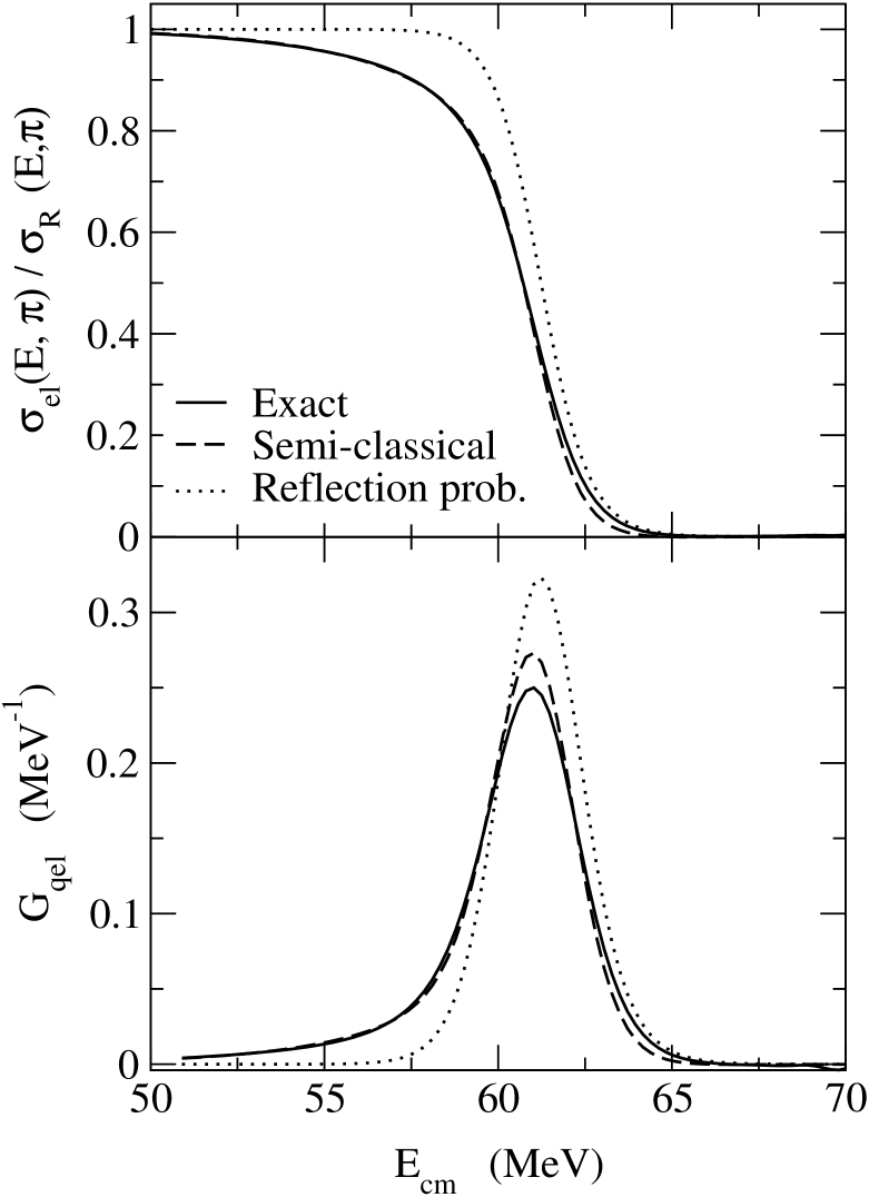
FIG. 1.: The ratio of elastic scattering to the Rutherford cross section at $\theta=\pi$ (upper panel) and the quasi-elastic test function $G_{\rm qel}(E)=-d/dE(\sigma_{\rm el}/\sigma_{R})$ (lower panel) for the ¹⁶O + ¹⁴⁴Sm reaction. The solid line is the exact solution of the optical potential, while the dashed line is obtained with the semi-classical perturbation theory. The dotted line denotes the reflection probability $R(E)=|S(E)|^{2}$ for $s$-wave scattering.

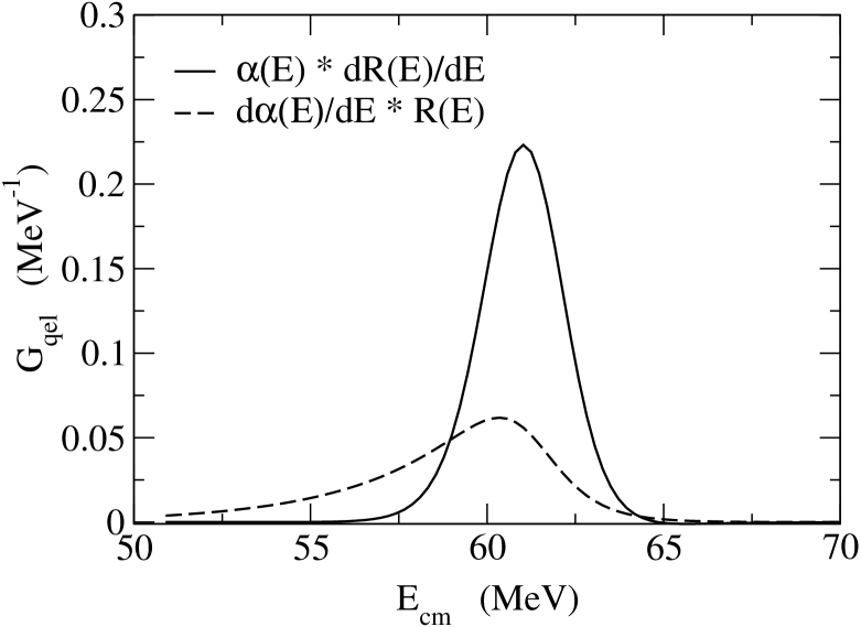
FIG. 2.: Two separate contributions to the quasi-elastic test function. The solid line shows the function $\alpha(E)\cdot dR(E)/dE$, while the dashed line shows $d\alpha(E)/dE\cdot R(E)$, where $\alpha(E)$ and $R(E)$ are the nuclear distortion function and the reflection probability, respectively.

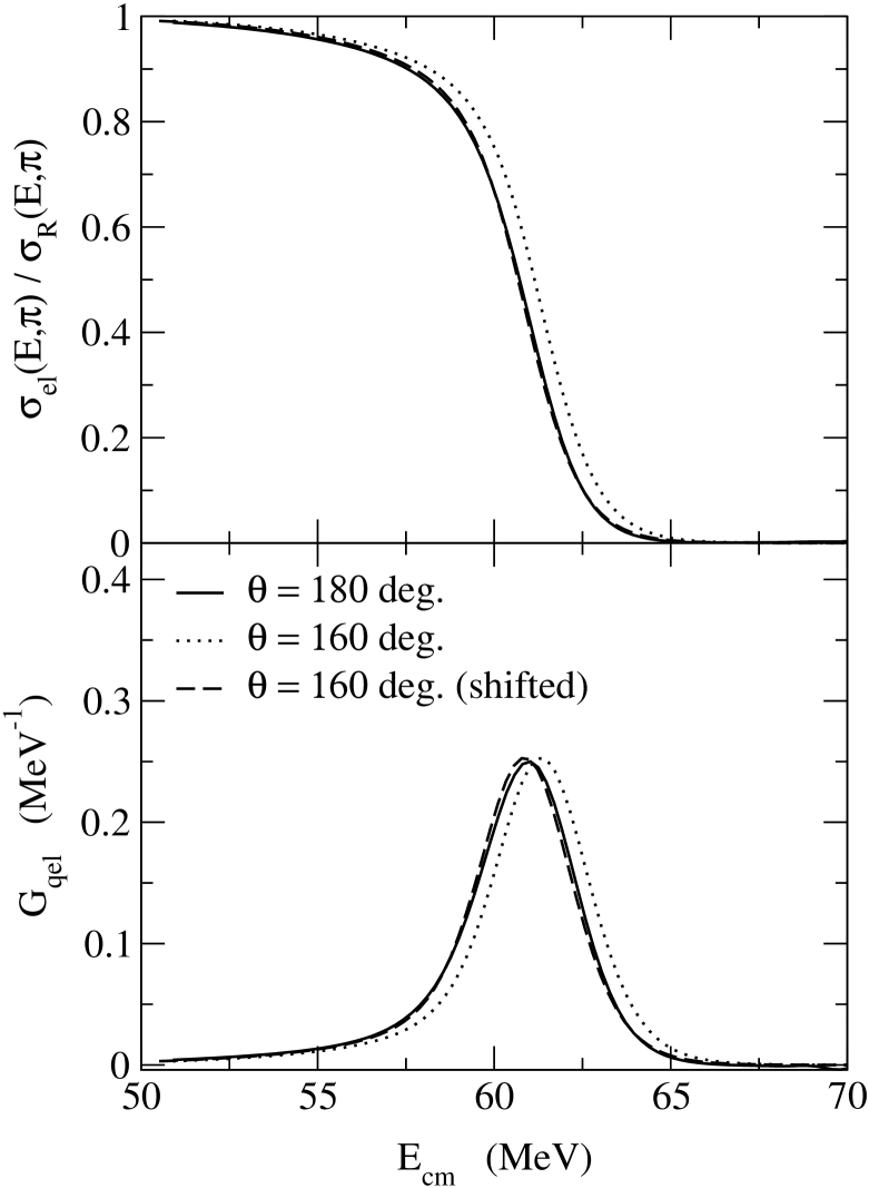
FIG. 3.: Comparison of the ratio $\sigma_{\rm el}/\sigma_{R}$ (upper panel) and its energy derivative $-d/dE(\sigma_{\rm el}/\sigma_{R})$ (lower panel) evaluated at two different scattering angles. The solid line is for $\theta=\pi$, while the dotted line is for $\theta=160^{\rm o}$. The dashed line is the same as the dotted line, but is shifted in energy by an amount equal to the centrifugal potential evaluated at the distance of closest approach of the Rutherford trajectory.

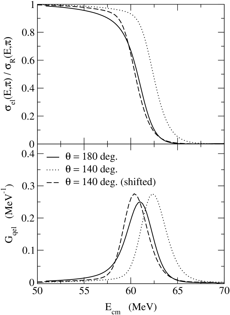
FIG. 4.: The same as fig.3, but for $\theta=140^{\rm o}$.

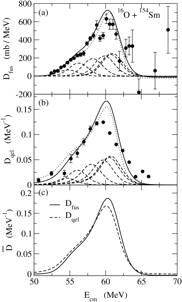
FIG. 5.: (a) The fusion barrier distribution $D_{\rm fus}(E)=d^{2}(E\sigma_{\rm fus})/dE^{2}$ for the ¹⁶O + ¹⁵⁴Sm reaction. The solid line is obtained with the orientation-integrated formula with $\beta_{2}=0.306$ and $\beta_{4}$= 0.05. The dashed lines indicate the contributions from the six individual eigenbarriers. These lines are obtained by using a Woods-Saxon potential with a surface diffuseness parameter $a$ of 0.65 fm. The dotted line is the fusion barrier distribution calculated with a potential which has $a$ = 1.05 fm. Experimental data are taken from Ref. [5]. (b) Same as Fig. 5(a), but for the quasi-elastic barrier distribution $D_{\rm qel}(E)=-d[\sigma_{\rm qel}(E,\pi)/\sigma_{R}(E,\pi)]/dE$. Experimental data are from Ref. [8]. (c) Comparison between the barrier distribution for fusion (solid line) and that for quasi-elastic scattering (dashed line). These functions are both normalized to unit area in the energy interval between 50 and 70 MeV.

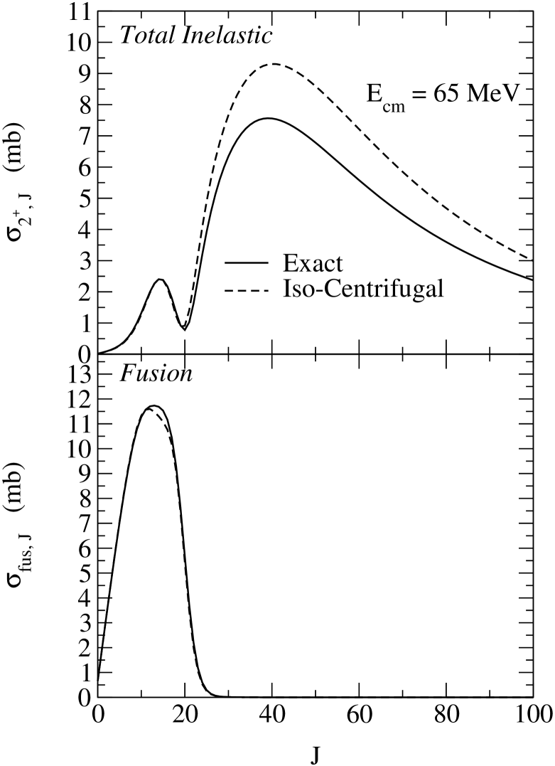
FIG. 6.: The effect of a quadrupole-phonon excitation in the target nucleus on the partial cross sections for the ¹⁶O + ¹⁴⁴Sm reaction at $E_{\rm cm}$=65 MeV. The upper and the lower panels show the angle-integrated inelastic scattering and the fusion cross sections, respectively. The solid line is the solution of the coupled-channels equations with the full angular momentum coupling, while the dashed line is obtained in the isocentrifugal approximation.

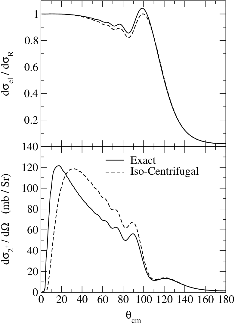
FIG. 7.: The angular distributions for the elastic (upper panel) and the inelastic (lower panel) scattering for the ¹⁶O + ¹⁴⁴Sm reaction at $E_{cm}$=65 MeV. The significance of each line is the same as in Fig. 5.

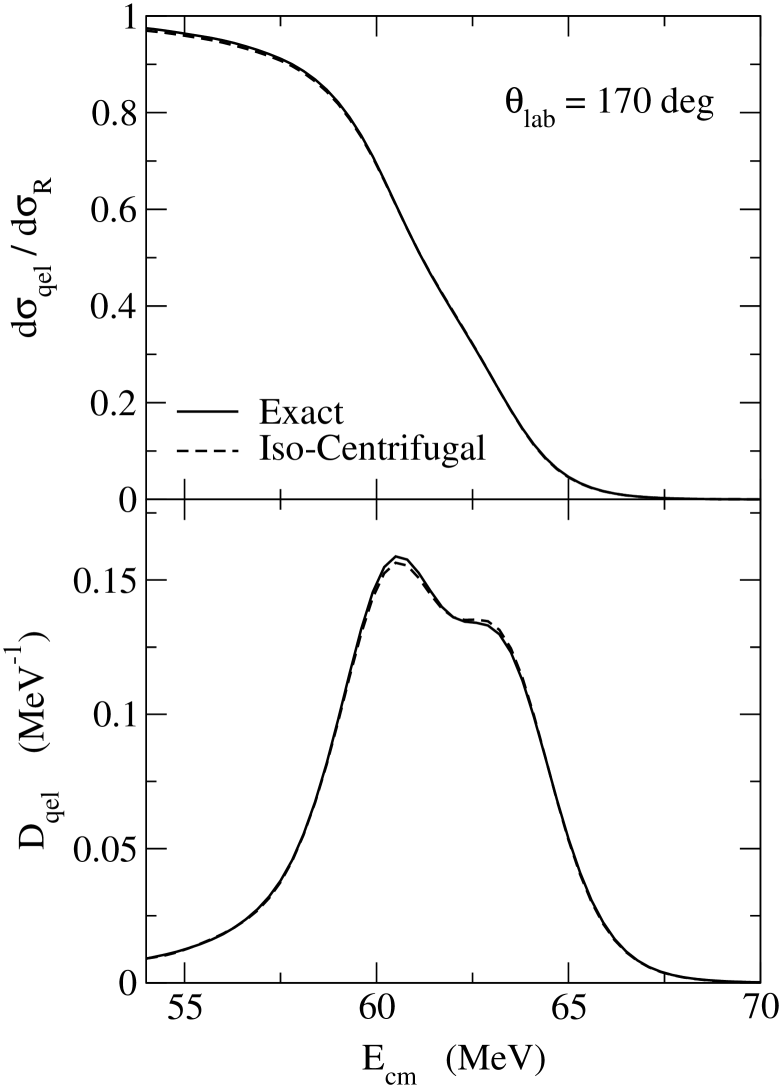
FIG. 8.: The excitation function for quasi-elastic scattering (upper panel) and the quasi-elastic barrier distribution (lower panel) for the ¹⁶O + ¹⁴⁴Sm reaction calculated at $\theta=170^{\rm o}$ in the laboratory frame. The significance of each line is the same as in Fig. 5.

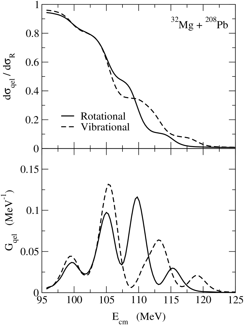
FIG. 9.: The excitation function for quasi-elastic scattering (upper panel) and the quasi-elastic barrier distribution (lower panel) for the ³²Mg + ²⁰⁸Pb reaction around the Coulomb barrier. The solid and the dashed lines are the results of coupled-channels calculations which assume that ³²Mg is a rotational and a vibrational nucleus, respectively. The single octupole-phonon excitation in ²⁰⁸Pb is also included in the calculations.

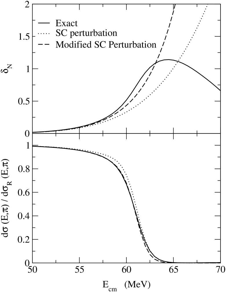
FIG. 10.: Comparison of the semi-classical formulae with the exact solution for the ¹⁶O+¹⁴⁴Sm reaction. The upper and the lower panels show the nuclear phase shift and the ratio of the elastic to the Rutherford cross sections at the scattering angle $\pi$, respectively. The solid line is obtained by numerically integrating the Schrödinger equation, while the dotted line is the result of the primitive semi-classical perturbation theory, Eqs. (A11) and (A12). The dashed line indicates the result of the semi-classical perturbation theory which takes into account the effect of nuclear distortion of the classical trajectory, Eqs. (A16) and (10).

REFERENCES

- [1] M. Dasgupta, D.J. Hinde, N. Rowley, and A.M. Stefanini, Annu. Rev. Nucl. Part. Sci. 48, 401 (1998).
- [2] A.B. Balantekin and N. Takigawa, Rev. Mod. Phys. 70, 77 (1998).
- [3] C.H. Dasso, S. Landowne, and A. Winther, Nucl. Phys. A405 (1983) 381; A407 (1983) 221.
- [4] N. Rowley, G.R. Satchler, and P.H. Stelson, Phys. Lett. B254, 25 (1991).
- [5] J.R. Leigh, M. Dasgupta, D.J. Hinde, J.C. Mein, C.R. Morton, R.C. Lemmon, J.P. Lestone, J.O. Newton, H. Timmers, J.X. Wei, and N. Rowley, Phys. Rev. C52, 3151 (1995).
- [6] A.M. Stefanini, D. Ackermann, L. Corradi, D.R. Napoli, C. Petrache, P. Spolaore, P. Bednarczyk, H.Q. Zhang, S. Beghini, G. Montagnoli, L. Mueller, F. Scarlassara, G.F. Segato, F. Soramel, and N. Rowley, Phys. Rev. Lett. 74, 864(1995).
- [7] M.V. Andres, N. Rowley, and M.A. Nagarajan, Phys. Lett. 202B, 292 (1988).
- [8] H. Timmers, J.R. Leigh, M. Dasgupta, D.J. Hinde, R.C. Lemmon, J.C. Mein, C.R. Morton, J.O. Newton, and N. Rowley, Nucl. Phys. A584, 190 (1995).
- [9] N. Rowley, Phys. of Atom. Nucl., 66, 1450 (2003).
- [10] E. Piasecki, M. Kowalczyk, K. Piasecki, L. Swiderski, J. Srebrny, M. Witecki, F. Carstoiu, W. Czarnacki, K. Rusek, J. Iwanicki, J. Jastrzebski, M. Kisielinski, A. Kordyasz, A. Stolarz, J. Tys, T. Krogulski, and N. Rowley, Phys. Rev. C65, 054611 (2002).
- [11] D.M. Brink, Semi-Classical Methods for Nucleus-Nucleus Scattering (Cambridge University Press, Cambridge, England, 1985).
- [12] S. Landowne and H.H. Wolter, Nucl. Phys. A351, 171 (1981).
- [13] R. Lindsay and N. Rowley, J. Phys. G10, 805 (1984).
- [14] M.A. Nagarajan, N. Rowley, and R. Lindsay, J. Phys. G12, 529 (1986).
- [15] M.A. Nagarajan, A.B. Balantekin, and N. Takigawa, Phys. Rev. C34, 894 (1986).
- [16] K. Hagino, N. Takigawa, A.B. Balantekin, and J.R. Bennett, Phys. Rev. C52, 286 (1995).
- [17] H. Esbensen, S. Landowne, and C. Price, Phys. Rev. C36, 1216 (1987); C36, 2359 (1987).
- [18] O. Tanimura, Phys. Rev. C35, 1600 (1987); Z. Phys. A327, 413 (1987).
- [19] N. Takigawa, F. Michel, A.B. Balantekin, and G. Reidemeister, Phys. Rev. C44, 477 (1991).
- [20] Y. Alhassid and H. Attias, Nucl. Phys. A577, 709 (1994).
- [21] J. Gomez-Camacho, M.V. Andres, and M.A. Nagarajan, Nucl. Phys. A580, 156 (1994).
- [22] K. Hagino, N. Takigawa, and A.B. Balantekin, Phys. Rev. C56, 2104 (1997).
- [23] C.Y. Wong, Phys. Rev. Lett. 31, 766 (1973).
- [24] D.M. Brink and G.R. Satchler, J. Phys. G7, 43 (1981).
- [25] K. Hagino, N. Rowley, and A.T. Kruppa, Comp. Phys. Comm. 123, 143 (1999).
- [26] T. Rumin, K. Hagino, and N. Takigawa, Phys. Rev. C63, 044603 (2001).
- [27] K. Hagino, N. Rowley, and M. Dasgupta, Phys. Rev. C67, 054603 (2003).
- [28] K. Hagino, N. Takigawa, M. Dasgupta, D.J. Hinde, and J.R. Leigh, Phys. Rev. C55, 276 (1997).
- [29] C. Signorini, Nucl. Phys. A693, 190 (2001).
- [30] C. Signorini, A. Yoshida, Y. Watanabe, D. Pierroutsakou, L. Stroe, T. Fukuda, M. Mazzocco, N. Fukuda, Y. Mizoi, M. Ishihara, H. Sakurai, A. Diaz-Torres, and K. Hagino, (to be published).
- [31] A. Yoshida, C. Signorini, T. Fukuda, Y. Watanabe, N. Aoi, M. Hirai, M. Ishihara, H. Kobinata, Y. Mizoi, L. Mueller, Y. Nagashima, J. Nakano, T. Nomura, Y.H. Pu, and F. Scarlassara, Phys. Lett. B389, 457 (1996).
- [32] M. Trotta, J.L. Sida, N. Alamanos, A. Andreyev, F. Auger, D.L. Balabanski, C. Borcea, N. Coulier, A. Drouart, D.J.C. Durand, G. Georgiev, A. Gillibert, J.D. Hinnerfeld, M. Huyse, C. Jouanne, V. Lapoux, A. Lepine, A. Lumbroso, F. Marie, A. Musumarra, G. Neyens, S. Ottini, R. Raabe, S. Ternier, P. Van Duppen, K. Vyvery, C. Volant, and R. Wolski, Phys. Rev. Lett. 84, 2342 (2000).
- [33] J.F. Liang, D. Shapira, C.J. Gross, J.R. Beene, J.D. Bierman, A. Galindo-Uribarri, J. Gomez del Campo, P.A. Hausladen, Y. Larochelle, W. Loveland, P.E. Mueller, D. Peterson, D.C. Radford, D.W. Stracener, and R.L. Varner, Phys. Rev. Lett. 91, 152701 (2003).
- [34] J. Al-Khalili and F. Nunes, J. Phys. G29, R89 (2003).
- [35] T. Motobayashi, Y. Ikeda, Y. Ando, K. Ieki, M. Inoue, N. Iwasa, T. Kikuchi, M. Kurokawa, S. Moriya, S. Ogawa, H. Murakami, S. Shimoura, Y. Yanagisawa, T. Nakamura, Y. Watanabe, M. Ishihara, T. Teranishi, H. Okuno, and R.F. Casten, Phys. Lett. B346, 9 (1995).
- [36] V. Chiste, A. Gillibert, A. Lepine-Szily, N. Alamanos, F. Auger, J. Barrette, F. Braga, M.D. Cortina-Gil, Z. Dlouhy, V. Lapoux, M. Lewitowicz, R. Lichtenthäler, R. Liguori Neto, S.M. Lukyanov, M. MacCormick, F. Marie, W. Mittig, F. de Oliveira Santos, N.A. Orr, A.N. Ostrowski, S. Ottini, A. Pakou, Yu.E. Penionzhkevich, P. Roussel-Chomaz, J.L. Sida, Phys. Lett. B514, 233 (2001).
- [37] K. Yoneda, H. Sakurai, T. Gomi, T. Motobayashi, N. Aoi, N. Fukuda, U. Futakami, Z. Gacsi, Y. Higurashi, N. Imai, N. Iwasa, H. Iwasaki, T. Kubo, M. Kunibu, M. Kurokawa, Z. Liu, T. Minemura, A. Saito, M. Serata, S. Shimoura, S. Takeuchi, Y.X. Watanabe, K. Yamada, Y. Yagamisawa, K. Yogo, A. Yoshida, and M. Ishihara, Phys. Lett. B499, 233 (2001).
- [38] P.-G. Reinhard, D.J. Dean, W. Nazarewicz, J. Dobaczewski, J.A. Maruhn, and M.R. Strayer, Phys. Rev. C60, 014316 (1999).
- [39] M. Yamagami and Nguyen Van Giai, e-print: nucl-th/0307051.
- [40] C.R. Morton, A.C. Berriman, M. Dasgupta, D.J. Hinde, J.O. Newton, K. Hagino, and I.J. Thompson, Phys. Rev. C60,44608 (1999).
- [41] O. Akyüz and A. Winther, in: Proc. Enrico Fermi Intern. School of Physics 1979, eds. R. A. Broglia, C. H. Dasso and R. Richi (North-Holland, Amsterdam, 1981).
- [42] K. Hagino and N. Rowley, (unpublished).
- [43] D.M. Brink and N. Takigawa, Nucl. Phys. A279, 159 (1977).