The Shell Model as Unified View of Nuclear Structure

Abstract

The last decade has witnessed both quantitative and qualitative progresses in Shell Model studies, which have resulted in remarkable gains in our understanding of the structure of the nucleus. Indeed, it is now possible to diagonalize matrices in determinantal spaces of dimensionality up to $10^{9}$ using the Lanczos tridiagonal construction, whose formal and numerical aspects we will analyze. Besides, many new approximation methods have been developed in order to overcome the dimensionality limitations. Furthermore, new effective nucleon-nucleon interactions have been constructed that contain both two and three-body contributions. The former are derived from realistic potentials (i.e., consistent with two nucleon data). The latter incorporate the pure monopole terms necessary to correct the bad saturation and shell-formation properties of the realistic two-body forces. This combination appears to solve a number of hitherto puzzling problems. In the present review we will concentrate on those results which illustrate the global features of the approach: the universality of the effective interaction and the capacity of the Shell Model to describe simultaneously all the manifestations of the nuclear dynamics either of single particle or collective nature. We will also treat in some detail the problems associated with rotational motion, the origin of quenching of the Gamow Teller transitions, the double $\beta$-decays, the effect of isospin non conserving nuclear forces, and the specificities of the very neutron rich nuclei. Many other calculations—that appear to have “merely” spectroscopic interest—are touched upon briefly, although we are fully aware that much of the credibility of the Shell Model rests on them.

I Introduction

In the early days of nuclear physics, the nucleus, composed of strongly interacting neutrons and protons confined in a very small volume, didn’t appear as a system to which the shell model, so successful in the atoms, could be of much relevance. Other descriptions—based on the analogy with a charged liquid drop—seemed more natural. However, experimental evidence of independent particle behavior in nuclei soon began to accumulate, such as the extra binding related to some precise values of the number of neutrons and protons (magic numbers) and the systematics of spins and parities.

The existence of shell structure in nuclei had already been noticed in the thirties but it took more than a decade and numerous papers (see Elliott and Lane, 1957, for the early history) before the correct prescription was found by Mayer (1949) and Axel, Jensen, and Suess (1949). To explain the regularities of the nuclear properties associated to “magic numbers”—i.e., specific values of the number of protons $Z$ and neutrons $N$—the authors proposed a model of independent nucleons confined by a surface corrected, isotropic harmonic oscillator, plus a strong attractive spin-orbit term,

$$U(r)=\frac{1}{2}\;\hbar\omega\;r^{2}+D\;\vec{l}\;^{2}+C\;\vec{l}\cdot\vec{s}.$$ (1)

In modern language this proposal amounts to assume that the main effect of the two-body nucleon-nucleon interactions is to generate a spherical mean field. The wave function of the ground state of a given nucleus is then the product of one Slater determinant for the protons and another for the neutrons, obtained by filling the lowest subshells (or “orbits”) of the potential. This primordial shell model is nowadays called “independent particle model” (IPM) or, “naive” shell model. Its foundation was pioneered by Brueckner (1954) who showed how the short range nucleon-nucleon repulsion combined with the Pauli principle could lead to nearly independent particle motion.

As the number of protons and neutrons depart from the magic numbers it becomes indispensable to include in some way the “residual” two-body interaction, to break the degeneracies inherent to the filling of orbits with two or more nucleons. At this point difficulties accumulate: “Jensen himself never lost his skeptical attitude towards the extension of the single-particle model to include the dynamics of several nucleons outside closed shells in terms of a residual interaction” (Weidenmüller, 1990). Nonetheless, some physicists chose to persist. One of our purposes is to explain and illustrate why it was worth persisting. The keypoint is that passage from the IPM to the interacting shell model, the shell model (SM) for short, is conceptually simple but difficult in practice. In the next section we succinctly review the steps involved. Our aim is to give the reader an overall view of the Shell Model as a sub-discipline of the Many Body problem. “Inverted commas” are used for terms of the nuclear jargon when they appear for the first time. The rest of the introduction will sketch the competing views of nuclear structure and establish their connections with the shell model. Throughout, the reader will be directed to the sections of this review where specific topics are discussed.

I.1 The three pillars of the shell model

The strict validity of the IPM may be limited to closed shells (and single particle –or hole– states built on them), but it provides a framework with two important components that help in dealing with more complex situations. One is of mathematical nature: the oscillator orbits define a basis of Slater determinants, the $m$-scheme, in which to formulate the Schrödinger problem in the occupation number representation (Fock space). It is important to realize that the oscillator basis is relevant, not so much because it provides an approximation to the individual nucleon wave-functions, but because it provides the natural quantization condition for self-bound systems.

Then, the many-body problem becomes one of diagonalizing a simple matrix. We have a set of determinantal states for $A$ particles, $a^{\dagger}_{i1}\ldots a^{\dagger}_{iA}|0\rangle=|\phi_{I}\rangle$, and a Hamiltonian containing kinetic ${\cal K}$ and potential energies ${\cal V}$

$${\cal H}=\sum_{ij}{\cal K}_{ij}\,a^{\dagger}_{i}a_{j}-\sum_{i\leq j\,k\leq l}{\cal V}_{ijkl}\,a^{\dagger}_{i}a^{\dagger}_{j}a_{k}a_{l}$$ (2)

that adds one or two particles in orbits $i,\,j$ and removes one or two from orbits $k,\,l$, subject to the Pauli principle ($\{a_{i}^{\dagger}a_{j}\}=\delta_{ij}$). The eigensolutions of the problem $|\Phi_{\alpha}\rangle=\sum_{I}\,c_{I,\alpha}|\phi_{I}\rangle$, are the result of diagonalizing the matrix $\langle\phi_{I}|{\cal H}|\phi_{I^{\prime}}\rangle$ whose off-diagonal elements are either 0 or $\pm{\cal V}_{ijkl}$. However, the dimensionalities of the matrices—though not infinite, since a cutoff is inherent to a non-relativistic approach—are so large as to make the problem intractable, except for the lightest nuclei. Stated in these terms, the nuclear many body problem does not differ much from other many fermion problems in condensed matter, quantum liquids or cluster physics; with which it shares quite often concepts and techniques. The differences come from the interactions, which in the nuclear case are particularly complicated, but paradoxically quite weak, in the sense that they produce sufficiently little mixing of basic states so as to make the zeroth order approximations bear already a significant resemblance with reality.

This is the second far-reaching –physical– component of the IPM: the basis can be taken to be small enough as to be, often, tractable. Here some elementary definitions are needed: The (neutron and proton) major oscillator shells of principal quantum number $p=0,\,1,\,2,\,3\ldots$, called $s,\,p,\,sd,\,pf\ldots$ respectively, of energy $\hbar\omega(p+3/2)$, contain orbits of total angular momentum $j=1/2,\,3/2\ldots p+1/2$, each with its possible $j_{z}$ projections, for a total degeneracy $D_{j}=2j+1$ for each subshell, and $D_{p}=(p+1)(p+2)$ for the major shells (One should not confuse the $p=1$ shell —$p$-shell in the old spectroscopic notation—with the generic harmonic oscillator shell of energy $\hbar\omega(p+3/2)$).

When for a given nucleus the particles are restricted to have the lowest possible values of $p$ compatible with the Pauli principle, we speak of a 0$\hbar\omega$ space. When the many-body states are allowed to have components involving basis states with up to $N$ oscillator quanta more than those pertaining to the 0$\hbar\omega$ space we speak of a $N$$\hbar\omega$ space (often refered as “no core”)

For nuclei up to $A\approx 60$, the major oscillator shells provide physically meaningful 0$\hbar\omega$ spaces. The simplest possible example will suggest why this is so. Start from the first of the magic numbers $N=Z=2$; ⁴He is no doubt a closed shell. Adding one particle should produce a pair of single-particle levels: $p_{3/2}$ and $p_{1/2}$. Indeed, this is what is found in ⁵He and ⁵Li. What about ⁶Li? The lowest configuration, $p_{3/2}^{2}$, should produce four states of angular momentum and isospin $JT=01,10,21,30$. They are experimentaly observed. There is also a $JT=20$ level that requires the $p_{3/2}\,p_{1/2}$ configuration. Hence the idea of choosing as basis $p^{m}$ ($p$ stands generically for $p_{3/2}\,p_{1/2}$) for nuclei up to the next closure $N=Z=8$, i.e., ¹⁶O. Obviously, the general Hamiltonian in (2) must be transformed into an “effective” one adapted to the restricted basis (the “valence space”). When this is done, the results are very satisfactory Cohen and Kurath (1965). The argument extends to the $sd$ and $pf$ shells.

By now, we have identified two of the three “pillars” of the Shell Model: a good valence space and an effective interaction adapted to it. The third is a shell model code capable of coping with the secular problem. In Section I.3 we shall examine the reasons for the success of the classical 0$\hbar\omega\,$ SM spaces and propose extensions capable of dealing with more general cases. The interaction will touched upon in Section I.2.3 and discussed at length in Section II. The codes will be the subject of Section III.

I.2 The competing views of nuclear structure

Because Shell Model work is so computer-intensive, it is instructive to compare its history and recent developments with the competing—or alternative—views of nuclear structure that demand less (or no) computing power.

I.2.1 Collective vs. Microscopic

The early SM was hard to reconcile with the idea of the compound nucleus and the success of the liquid drop model. With the discovery of rotational motion Bohr (1952); Bohr and Mottelson (1953) which was at first as surprising as the IPM, the reconciliation became apparently harder. It came with the realization that collective rotors are associated with “intrinsic states” very well approximated by deformed mean field determinants Nilsson (1955), from which the exact eigenstates can be extracted by projection to good angular momentum Peierls and Yoccoz (1957); an early and spectacular example of spontaneous symmetry breaking. By further introducing nuclear superfluidity Bohr et al. (1958), the unified model was born, a basic paradigm that remains valid.

Compared with the impressive architecture of the unified model, what the SM could offer were some striking but isolated examples which pointed to the soundness of a many-particle description. Among them, let us mention the elegant work of Talmi and Unna (1960), the $f_{7/2}^{n}$ model of McCullen, Bayman, and Zamick (1964)—probably the first successful diagonalization involving both neutrons and protons—and the Cohen and Kurath (1965) fit to the $p$ shell, the first of the classical 0$\hbar\omega$ regions. It is worth noting that this calculation involved spaces of $m$-scheme dimensionalities, $d_{m}$, of the order of 100, while at fixed total angular momentum and isospin $d_{JT}\approx 10$.

The microscopic origin of rotational motion was found by Elliott (1958a, b). The interest of this contribution was immediately recognized but it took quite a few years to realize that Elliott’s quadrupole force and the underlying SU(3) symmetry were the foundation, rather than an example, of rotational motion (see Section VI).

It is fair to say that for almost twenty years after its inception, in the mind of many physicists, the shell model still suffered from an implicit separation of roles, which assigned it the task of accurately describing a few specially important nuclei, while the overall coverage of the nuclear chart was understood to be the domain of the unified model.

A somehow intermediate path was opened by the well known Interacting Boson Model of Arima and Iachello (1975) and its developments, that we do not touch here. The interested reader can find the details in Iachello and Arima (1987).

I.2.2 Mean field vs Diagonalizations

The first realistic matrix elements of Kuo and Brown (1966) and the first modern shell model code by French, Halbert, McGrory, and Wong (1969) came almost simultaneously, and opened the way for the first generation of “large scale” calculations, which at the time meant $d_{JT}\approx 100$-600. They made it possible to describe the neighborhood of ¹⁶O Zuker, Buck, and McGrory (1968) and the lower part of the $sd$ shell Halbert et al. (1971). However, the increases in tractable dimensionalities were insufficient to promote the shell model to the status of a general description, and the role-separation mentioned above persisted. Moreover the work done exhibited serious problems which could be traced to the realistic matrix elements themselves (see next Section I.2.3).

However, a fundamental idea emerged at the time: the existence of an underlying universal two-body interaction, which could allow a replacement of the unified model description by a fully microscopic one, based on mean-field theory. The first breakthrough came when Baranger and Kumar (1968) proposed a new form of the unified model by showing that Elliott’s quadrupole force could be somehow derived from the Kuo-Brown matrix elements. Adding a pairing interaction and a spherical mean field they proceeded to perform Hartree Fock Bogoliubov calculations in the first of a successful series of papers Kumar and Baranger (1968). Their work could be described as shell model by other means, as it was restricted to valence spaces of two contiguous major shells.

This limitation was overcome when Vautherin and Brink (1972) and Dechargé and Gogny (1980) initiated the two families of Hartree Fock (HF) calculations (Skyrme and Gogny for short) that remain to this day the only tools capable of giving microscopic descriptions throughout the periodic table. They were later joined by the relativistic HF approach Serot and Walecka (1986). (For a review of the three variants see Bender, Heenen, and Reinhard, 2003b). See also Péru, Girod, and Berger (2000) and Rodriguez-Guzmán, Egido, and Robledo (2000) and references therein for recent work with the Gogny force, the one for which closest contact with realistic interactions and the shell model can be established (Sections VI.1 and II.4).

Since single determinantal states can hardly be expected accurately to describe many body solutions, everybody admits the need of going beyond the mean field. Nevertheless, as it provides such a good approximation to the wavefunctions (typically about 50%) it suggests efficient truncation schemes, as will be explained in Sections IV.2.1 and IV.2.2.

I.2.3 Realistic vs Phenomenological

Nowadays, many regions remain outside the direct reach of the Shell Model, but enough has happened in the last decade to transform it into a unified view. Many steps—outlined in the next Section I.4—are needed to substantiate this claim. Here we introduce the first: A unified view requires a unique interaction. Its free parameters must be few and well defined, so as to make the calculations independent of the quantities they are meant to explain. Here, because we touch upon a different competing view, of special interest for shell model experts, we have to recall the remarks at the end of the first paragraph of the preceding Section I.2.2:

The exciting prospect that realistic matrix elements could lead to parameter-free spectroscopy did not materialize. As the growing sophistication of numerical methods allowed to treat an increasing number of particles in the $sd$ shell, the results became disastrous. Then, two schools of thought on the status of phenomenological corrections emerged: In one of them, all matrix elements were considered to be free parameters. In the other, only average matrix elements (“centroids”)—related to the bad saturation and shell formation properties of the two-body potentials—needed to be fitted (the monopole way). The former lead to the “Universal $sd$” (USD) interaction Wildenthal (1984), that enjoyed an immense success and for ten years set the standard for shell model calculations in a large valence space Brown and Wildenthal (1988), (see Brown, 2001, for a recent review). The second, which we adopt here, was initiated in Eduardo Pasquini PhD thesis (1976), where the first calculations in the full $pf$ shell, involving both neutrons and protons were done. Twenty years later, we know that the minimal monopole corrections proposed in his work are sufficient to provide results of a quality comparable to those of USD for nuclei in $f_{7/2}$ region.

However, there were still problems with the monopole way: they showed around and beyond ⁵⁶Ni, as well as in the impossibility to be competitive with USD in the $sd$ shell (note that USD contains non-monopole two-body corrections to the realistic matrix elements). The solution came about only recently with the introduction of three-body forces: This far reaching development will be explained in detail in Sections II, II.2 and V.1. We will only anticipate on the conclusions of these sections through two syllogisms. The first is: The case for realistic two-body interactions is so strong that we have to accept them as they are. Little is known about three-body forces except that they exist. Therefore problems with calculations involving only two body forces must be blamed on the absence of three body forces. This argument raises (at least) one question: What to make of all calculations, using only two-body forces, that give satisfactory results? The answer lies in the second syllogism: All clearly identifiable problems are of monopole origin. They can be solved reasonably well by phenomenological changes of the monopole matrix elements. Therefore, fitted interactions can differ from the realistic ones basically through monopole matrix elements. (We speak of R-compatibility in this case). The two syllogisms become fully consistent by noting that the inclusion of three-body monopole terms always improves the performance of the forces that adopt the monopole way.

For the 0$\hbar\omega$ spaces, the Cohen Kurath Cohen and Kurath (1965), the Chung Wildenthal Wildenthal and Chung (1979) and the FPD6 Richter et al. (1991) interactions turn out to be R-compatible. The USD Wildenthal (1984) interaction is R-incompatible. It will be of interest to analyze the recent set of $pf$-shell matrix elements (GXPF1), proposed by Honma et al. (2002), but not yet released.

I.3 The valence space

The choice of the valence space should reflect a basic physical fact: that the most significant components of the low lying states of nuclei can be accounted for by many-body states involving the excitation of particles in a few orbitals around the Fermi level. The history of the Shell Model is that of the interplay between experiment and theory to establish the validity of this concept. Our present understanding can be roughly summed up by saying that “few” mean essentially one or two contiguous major shells.

For a single major shell, the classical 0$\hbar\omega$ spaces, exact solutions are now available from which instructive conclusions can be drawn. Consider, for instance,the spectrum of ⁴¹Ca from which we want to extract the single-particle states of the $pf$ shell. Remember that in ⁵Li we expected to find two states, and indeed found two. Now, in principle, we expect four states. They are certainly in the data. However, they must be retrieved from a jungle of some 140 levels seen below 7 MeV. Moreover, the $f_{7/2}$ ground state is the only one that is a pure single particle state, the other ones are split, even severely in the case of the highest ($f_{5/2}$)  Endt and van der Leun (1990). (Section V.2.1 contains an interesting example of the splitting mechanism). Thus, how can we expect the $pf$ shell to be a good valence space? For few particles above ⁴⁰Ca it is certainly not. However, as we report in this work, it turns out that above $A=46$, the lowest $(pf)^{m}$ configurations  are sufficiently detached from all others so as to generate wavefunctions that can evolve to the exact ones through low order perturbation theory.

The ultimate ambition of Shell Model theory is to get exact solutions. The ones provided by the sole valence space are, so to speak, the tip of the iceberg in terms of number of basic states involved. The rest may be so well hidden as to make us believe in the literal validity of the shell model description in a restricted valence space. For instance, the magic closed shells are good valence spaces consisting of a single state. This does not mean that a magic nucleus is 100% closed shell: 50 or 60% should be enough, as we shall see in Section IV.2.1. In section V.3.1 it will be argued that the 0$\hbar\omega\,$ valence spaces account for basically the same percentage of the full wavefunctions. Conceptually the valence space may be thought as defining a representation intermediate between the Schrödinger one (the operators are fixed and the wavefunction contains all the information) and the Heisenberg one (the reverse is true).

At best, 0$\hbar\omega$ spaces can describe only a limited number of low-lying states of the same (“natural”) parity. Two contiguous major shells can most certainly cope with all levels of interest but they lead to intractably large spaces and suffer from a “Center of Mass problem” (analyzed in Appendix C). Here, a physically sound pruning of the space is suggested by the IPM. What made the success of the model is the explanation of the observed magic numbers generated by the spin-orbit term, as opposed to the HO (harmonic oscillator) ones (for shell formation see Section II.2.2). If we separate a major shell as HO($p$)$=p_{>}\oplus r_{p}$, where $p_{>}$ is the largest subshell having $j=p+1/2$, and $r_{p}$ is the “rest” of the HO $p$-shell, we can define the EI (extruder-intruder) spaces as EI($p$)$=r_{p}\oplus(p+1)_{>}$: The $(p+1)_{>}$ orbit is expelled from HO($p+1$) by the spin-orbit interaction and intrudes into HO($p$). The EI spaces are well established standards when only one “fluid” (proton or neutron) is active: The $Z$ or $N=28,\,50,\,82$ and 126 isotopes or isotones. These nuclei are “spherical”, amenable to exact diagonalizations and fairly well understood (see for example Abzouzi et al., 1991).

As soon as both fluids are active, “deformation” effects become appreciable, leading to “coexistence” between spherical and deformed states, and eventually to dominance of the latter. To cope with this situation we propose “Extended EI spaces” defined as EEI($p$)$=r_{p}\;\oplus\Delta_{p+1}$, where $\Delta_{p}=p_{>}\oplus(p_{>}-2)\oplus\ldots$, i.e., the $\Delta j=2$ sequence of orbits that contain $p_{>}$, which are needed to account for rotational motion as explained in Section VI. The EEI(1) ($p_{1/2},\,d_{5/2},\,s_{1/2}$) space was successful in describing the full low lying spectra for $A=15$-18 Zuker et al. (1968, 1969). It is only recently that the EEI(2) ($s_{1/2},\,d_{3/2},\,f_{7/2},\,p_{3/2}$) space (region around ⁴⁰Ca) has become tractable (see Sections VI.4 and VIII.3). EEI(3) is the natural space for the proton rich region centered in ⁸⁰Zr. For heavier nuclei exact diagonalizations are not possible but the EEI spaces provide simple (and excellent) estimates of quadrupole moments at the beginning of the well deformed regions (Section VI.3).

As we have presented it, the choice of valence space is primarily a matter of physics. In practice, when exact diagonalizations are impossible, truncations are introduced. They may be based on systematic approaches, such as approximation schemes discussed in Sections IV.2.1 and IV.2.2 or mean field methods mentioned in Section I.2.2, and analyzed in Section VI.1.

I.4 About this review: the unified view

We expect this review to highlight several unifying aspects common to the most recent successful shell model calculations:

a) An effective interaction connected with both the two and three nucleon bare forces.

b) The explanation of the global properties of nuclei via the monopole Hamiltonian.

c) The universality of the multipole Hamiltonian.

d) The description of the collective behavior in the laboratory frame, by means of the spherical shell model.

e) The description of resonances using the Lanczos strength function method.

Let us see now how this review is organized along these lines. References are only given for work that will not be mentioned later.

Section II. The basic tool in analyzing the interaction is the monopole-multipole separation. The former is in charge of saturation and shell properties; it can be thought as the correct generalization of Eq. (1). Monopole theory is scattered in many references. Only by the inclusion of three-body forces could a satisfactory formulation be achieved. As this is a very recent and fundamental development which makes possible a unified viewpoint of the monopole field concept, this section is largely devoted to it. The “residual” multipole force has been extensively described in a single reference which will be reviewed briefly and updated. The aim of the section is to show how the realistic interactions can be characterized by a small number of parameters.

Section III. The ANTOINE and NATHAN codes have made it possible to evolve from dimensionalities $d_{m}\sim 5\times 10^{4}$ in 1989 to $d_{m}\sim 10^{9},\,d_{J}\sim 10^{7}$ nowadays. Roughly half of the–order of magnitude–gains are due to increases in computing power. The rest comes from algorithmic advances in the construction of tridiagonal Lanczos matrices that will be described in this section.

Section IV. The Lanczos construction can be used to eliminate the “black box” aspect of the diagonalizations, to a large extent. We show how it can be related to the notions of partition function, evolution operator and level densities. Furthermore, it can be turned into a powerful truncation method by combining it to coupled cluster theory. Finally, it describes strength functions with maximal efficiency.

Section V. After describing the three body mechanism which solves the monopole problem that had plagued the classical 0$\hbar\omega$ calculations, some selected examples of $pf$ shell spectroscopy are presented. Special attention is given to Gamow Teller transitions, one of the main achievements of modern SM work.

Section VI. Another major recent achievement is the shell model description of rotational nuclei. The new generation of gamma detectors, Euroball and Gammasphere has made it possible to access high spin states in medium mass nuclei for which full 0$\hbar\omega$ calculations are available. Their remarkable harvest includes a large spectrum of collective manifestations which the spherical shell model can predict or explain as, for instance, deformed rotors, backbending, band terminations, yrast traps, etc. Configurations involving two major oscillator shells are also shown to account well for the appearance of superdeformed excited bands.

Section VII. A conjunction of factors make light and medium-light nuclei near the neutron drip line specially interesting: (a) They have recently come under intense experimental scrutiny. (b) They are amenable to shell model calculations, sometimes even exact no-core ones (c) They exhibit very interesting behavior, such as halos and sudden onset of deformation. (d) They achieve the highest $N/Z$ ratios attained. (e) When all (or most of) the valence particles are neutrons, the spherical shell model closures, dictated by the isovector channel of the nuclear interaction alone, may differ from those at the stability valley. These regions propose some exacting tests for the theoretical descriptions, that the conventional shell model calculations have passed satisfactorily. For nearly unbound nuclei, the SM description has to be supplemented by some refined extensions such as the shell model in the continuum, which falls outside the scope of this review. References to the subject can be found in Bennaceur et al. (1999, 2000), and in Id Betan et al. (2002); Michel et al. (2002, 2003) that deal with the Gamow shell model.

Section VIII. There is a characteristic of the Shell Model we have not yet stressed: it is the approach to nuclear structure that can give more precise quantitative information. SM wave functions are, in particular, of great use in other disciplines. For example: Weak decay rates are crucial for the understanding of several astrophysical processes, and neutrinoless $\beta\beta$ decay is one of the main sources of information about the neutrino masses. In both cases, shell model calculations play a central role. The last section deal with these subjects, and some others…

Appendix B contains a full derivation of the general form of the monopole field.

Two recent reviews by Brown (2001) and Otsuka et al. (2001b) have made it possible to simplify our task and avoid redundancies. However we did not feel dispensed from quoting and commenting in some detail important work that bears directly on the subjects we treat.

Sections II, IV and the Appendices are based on unpublished notes by APZ.

II The interaction

The following remarks from Abzouzi, Caurier, and Zuker (1991) still provide a good introduction to the subject:

“The use of realistic potentials (i.e., consistent with $NN$ scattering data) in shell-model calculation was pioneered by Kuo and Brown (1966). Of the enormous body of work that followed we would like to extract two observations. The first is that whatever the forces (hard or soft core, ancient or new) and the method of regularization (Brueckner $G$ matrix (Kuo and Brown, 1966; Kahana et al., 1969a), Sussex direct extraction (Elliott et al., 1968) or Jastrow correlations (Fiase et al., 1988)) the effective matrix elements are extraordinarily similar (Pasquini and Zuker, 1978; Rutsgi et al., 1971). The most recent results (Jiang et al., 1989) amount to a vindication of the work of Kuo and Brown. We take this similarity to be the great strength of the realistic interactions, since it confers on them a model-independent status as direct links to the phase shifts.

The second observation is that when used in shell-model calculations and compared with data these matrix elements give results that deteriorate rapidly as the number of particle increases (Halbert et al., 1971) and (Brown and Wildenthal, 1988). It was found (Pasquini and Zuker, 1978) that in the $pf$ shell a phenomenological cure, confirmed by exact diagonalizations up to A=48 (Caurier et al., 1994), amounts to very simple modifications of some average matrix elements ($centroids$) of the KB interaction (Kuo and Brown, 1968).”

In Abzouzi et al. (1991) very good spectroscopy in the $p$ and $sd$ shells could be obtained only through more radical changes in the centroids, involving substantial three-body (3b) terms. In 1991 it was hard to interpret them as effective and there were no sufficient grounds to claim that they were real.

Nowadays, the need of true 3b forces has become irrefutable: In the 1990 decade several two-body (2b) potentials were developed—Nijmegen I and II (Stoks et al., 1993), AV18 (Wiringa et al., 1995), CD-Bonn-(Machleidt et al., 1996)—that fit the $\approx 4300$ entries in the Nijmegen data base (Stoks et al., 1994) with $\chi^{2}\approx\,1$, and none of them seemed capable to predict perfectly the nucleon vector analyzing power in elastic $(N,d)$ scattering (the $A_{y}$ puzzle). Two recent additions to the family of high-precision 2b potentials—the charge-dependent “CD-Bonn” (Machleidt, 2001) and the chiral Idaho-A and B (Entem and Machleidt, 2002)—have dispelled any hopes of solving the $A_{y}$ puzzle with 2b-only interactions (Entem et al., 2002).

Furthermore, quasi-exact 2b Green Function Monte Carlo (GFMC) results (Pudliner et al., 1997; Wiringa et al., 2000) which provided acceptable spectra for $A\leq 8$ (though they had problems with binding energies and spin-orbit splittings), now encounter serious trouble in the spectrum of ¹⁰B, as found through the No Core Shell Model (NCSM) calculations of  Navrátil and Ormand (2002) and Caurier et al. (2002), confirmed by Pieper, Varga, and Wiringa (2002), who also show that the problems can be remedied to a large extent by introducing the new Illinois 3b potentials developed by Pieper et al. (2001).

It is seen that the trouble detected with a 2b-only description—with binding energies, spin-orbit splittings and spectra—is always related to centroids, which, once associated to operators that depend only on the number of particles in subshells, determine a “monopole” Hamiltonian ${\cal H}_{m}$ that is basically in charge of Hartree Fock selfconsistency. As we shall show, the full ${\cal H}$ can be separated rigorously as ${\cal H}={\cal H}_{m}+{\cal H}_{M}$. The multipole part ${\cal H}_{M}$ includes pairing, quadrupole and other forces responsible for collective behavior, and—as checked by many calculations—is well given by the 2b potentials.

The preceding paragraph amounts to rephrasing the two observations quoted at the beginning of this section with the proviso that the blame for discrepancies with experiment cannot be due to the—now nearly perfect—2b potentials. Hence the necessary “corrections” to ${\cal H}_{m}$ must have a 3b origin. Given that we have no complaint with ${\cal H}_{M}$, the primary problem is the monopole contribution to the 3b potentials. This is welcome because a full 3b treatment would render most shell model calculations impossible, while the phenomenological study of monopole behavior is quite simple. Furthermore it is quite justified because there is little ab initio knowledge of the 3b potentials. Therefore, whatever information that comes from nuclear data beyond A=3 is welcome.

In Shell Model calculations, the interaction appears as matrix elements, that soon become far more numerous than the number of parameters defining the realistic potentials. Our task will consist in analyzing the Hamiltonian in the oscillator representation (or Fock space) so as to understand its workings and simplify its form. In Section II.1 we sketch the theory of effective interactions. In Section II.2 it is explained how to construct from data a minimal ${\cal H}_{m}$, while Section II.3 will be devoted to extract from realistic forces the most important contributions to ${\cal H}_{M}$. The basic tools are symmetry and scaling arguments, the clean separation of bulk and shell effects and the reduction of ${\cal H}$ to sums of factorable terms (Dufour and Zuker, 1996).

II.1 Effective interactions

The Hamiltonian is written in an oscillator basis as

$${\cal H} = {\cal K}+\sum_{r\leq s,\;t\leq u,\;\Gamma}{{\cal V}}_{rstu}^{\Gamma}Z_{rs\Gamma}^{+}\cdot Z_{tu\Gamma}$$ (3)

$$+\sum_{r\leq s\leq t,\;u\leq v\leq w,\;\Gamma}{\cal V}_{rstuvw}^{\Gamma}Z_{rst\Gamma}^{+}\cdot Z_{uvw\Gamma},$$

where ${\cal K}$ is the kinetic energy, ${\cal V}_{\bm{rr^{\prime}}}^{\Gamma}$ the interaction matrix elements, $Z^{+}_{{\bm{r}}\Gamma}$ ( $Z_{{\bm{r}}\Gamma}$) create (annihilate) pairs (${\bm{r}}\equiv rs$) or triples (${\bm{r}}\equiv rst$) of particles in orbits ${\bm{r}}$, coupled to $\Gamma=JT$. Dots stand for scalar products. The basis and the matrix elements are large but never infinite.

The aim of an effective interaction theory is to reduce the secular problem in the large space to a smaller model space by treating perturbatively the coupling between them, thereby transforming the full potential, and its repulsive short distance behavior, into a smooth pseudopotential.

In what follows, if we have to distinguish between large ($N\hbar\omega$) and model spaces we use ${\cal H},\,{\cal K}\,{\rm and}\,{\cal V}$ for the pseudo-potential in the former and $H,\,K\,{\rm and}\,V$ for the effective interaction in the latter.

II.1.1 Theory and calculations

The general procedure to describe an exact eigenstate in a restricted space was obtained independently by Suzuki and Lee (1980) and Poves and Zuker (1981a). It consists in dividing the full space into model ($|i\rangle$) and external ($|\alpha\rangle$) determinants, and introducing a transformation that respects strict orthogonality between the spaces and decouples them exactly:

$$|\overline{\imath}\rangle=|i\rangle+\sum_{\alpha}A_{i\alpha}|\alpha\rangle\;\;|\overline{\alpha}\rangle=|\alpha\rangle-\sum_{i}A_{i\alpha}|i\rangle$$ (4)

$$\langle\overline{\imath}|\overline{\alpha}\rangle=0,\;\;A_{i\alpha}\;\text{is defined through}\;\;\langle\overline{\imath}|{\cal H}|\overline{\alpha}\rangle=0.$$ (5)

The idea is that the model space can produce one or several starting wavefunctions that can evolve to exact eigenstates through perturbative or coupled cluster evaluation of the amplitudes $A_{i\alpha}$, which can be viewed as matrix elements of a many body operator $A$. In coupled cluster theory (CCT or $\exp{S}$) (Coester and Kümmel (1960),  Kümmel et al. (1978)) one sets $A=\exp{S}$, where $S=S_{1}+S_{2}+\cdots+S_{k}$ is a sum of $k$-body (kb) operators. The decoupling condition $\langle\overline{\imath}|{\cal H}|\overline{\alpha}\rangle=0$ then leads to a set of coupled integral equations for the $S_{i}$ amplitudes. When the model space reduces to a single determinant, setting $S_{1}=0$ leads to Hartree Fock theory if all other amplitudes are neglected. The $S_{2}$ approximation contains both low order Brueckner theory (LOBT) and the random phase approximation (RPA) . In the presence of hard-core potentials, the priority is to screen them through LOBT, and the matrix elements contributing to the RPA are discarded. An important implementation of the theory was due to Zabolitzky, whose calculations for ⁴He, ¹⁶O and ⁴⁰Ca, included $S_{3}$ (Bethe Faddeev) and $S_{4}$ (Day Yacoubovsky) amplitudes (Kümmel, Lührmann, and Zabolitzky, 1978). This “Bochum truncation scheme” that retraces the history of nuclear matter theory has the drawback that at each level terms that one would like to keep are neglected.

The way out of this problem  Heisenberg and Mihaila (2000); Mihaila and Heisenberg (2000) consists on a new truncation scheme in which some approximations are made, but no terms are neglected, relying on the fact that the matrix elements are finite. The calculations of these authors for ¹⁶O (up to $S_{3}$) can be ranked with the quasi-exact GFMC and NCSM ones for lighter nuclei.

In the quasi-degenerate regime (many model states), the coupled cluster equations determine an effective interaction in the model space. The theory is much simplified if we enforce the decoupling condition for a single state whose exact wavefunction is written as

$$|\overline{ref}\rangle=(1+A_{1}+A_{2}+\dots)(1+B_{1}+B_{2}+\dots)|ref\rangle\\ =(1+C_{1}+C_{2}+\dots)|ref\rangle,\qquad C=\exp{S},$$ (6)

where $|ref\rangle$ is a model determinant. The internal amplitudes associated with the $B$ operators are those of an eigenstate obtained by diagonalizing $H_{eff}={\cal H}(1+A)$ in the model space. As it is always possible to eliminate the $A_{1}$ amplitude, at the $S_{2}$ level there is no coupling i.e., the effective interaction is a state independent G-matrix Zuker (1984), which has the advantage of providing an initialization for $H_{eff}$. Going to the $S_{3}$ level would be very hard, and we examine what has become standard practice.

The power of CCT is that it provides a unified framework for the two things we expect from decoupling: to smooth the repulsion and to incorporate long range correlations. The former demands jumps of say, 50$\hbar\omega$, the latter much less. Therefore it is convenient to treat them separately. Standard practice assumes that G-matrix elements can provide a smooth pseudopotential in some sufficiently large space, and then accounts for long range correlations through perturbation theory. The equation to be solved is

$$G_{ijkl}={\cal V}_{ijkl}-\sum_{\alpha\beta}\frac{{\cal V}_{ij\alpha\beta}G_{\alpha\beta kl}}{\epsilon_{\alpha}+\epsilon_{\beta}-\epsilon_{i}-\epsilon_{j}+\Delta},$$ (7)

where $ij$ and $kl$ now stand for orbits in the model space while in the pair $\alpha\beta$ at least one orbit is out of it, $\epsilon_{x}$ is an unperturbed (usually kinetic) energy, and $\Delta$ a free parameter called the “starting” energy. Hjorth-Jensen, Kuo, and Osnes (1995) describe in detail a sophisticated partition that amounts to having two model spaces, one large and one small.

In the NCSM calculations an $N\hbar\omega$ model space is chosen with $N\approx 6$-10. When initiated by Zheng et al. (1993) the pseudo-potential was a G-matrix with starting energy. Then the $\Delta$ dependence was eliminated either by arcane perturbative maneuvers, or by a truly interesting proposal: direct decoupling of 2b elements from a very large space Navrátil and Barrett (1996), further implemented by Navrátil, Vary, and Barrett (2000a), and extended to 3b effective forces Navrátil et al. (2000), Navrátil and Ormand (2002). It would be of interest to compare the resulting effective interactions to the Brueckner and Bethe Faddeev amplitudes obtained in a full $\exp{S}$ approach (which are also free of arbitrary starting energies).

A most valuable contribution of NCSM is the proof that it is possible to work with a pseudo-potential in $N\hbar\omega$ spaces. The method relies on exact diagonalizations. As they soon become prohibitive, in the future, CCT may become the standard approach: going to $S_{3}$ for $N=50$ (as Heisenberg and Mihaila did) is hard. For $N=10$ it should be much easier.

Another important NCSM indication is that the excitation spectra converge well before the full energy, which validates formally the $0\hbar\omega$ diagonalizations with rudimentary potentials and second order corrections.

The $0\hbar\omega$ results are very good for the spectra. However, to have a good pseudopotential to describe energies is not enough. The transition operators also need dressing. For some of them, notably $E2$, the dressing mechanism (coupling to 2$\hbar\omega\,$quadrupole excitations) has been well understood for years (see Dufour and Zuker, 1996, for a detailed analysis), and yields the, abundantly tested and confirmed, recipe of using effective charges of $\approx$ 1.5e for the protons and $\approx$ 0.5e for neutrons. For the Gamow Teller (GT) transitions, mediated by the spin-isospin $\sigma\tau_{\pm}$ operator the renormalization mechanism involves an overall “quenching” factor of 0.7–0.8 whose origin is far subtler. It will be examined in Sections V.3.1 and V.3.2. The interested reader may wish to consult them right away.

II.2 The monopole Hamiltonian

A many-body theory usually starts by separating the Hamiltonian into an “unperturbed” and a “residual” part, ${\cal H}={\cal H}_{0}+{\cal H}_{r}$. The traditional approach consists in choosing for ${\cal H}_{0}$ a one body (1b) single-particle field. Since ${\cal H}$ contains two and three-body (2b and 3b) components, the separation is not mathematically clean. Therefore, we propose the following

$${\cal H}={\cal H}_{m}+{\cal H}_{M},$$ (8)

where ${\cal H}_{m}$, the monopole Hamiltonian, contains ${\cal K}$ and all quadratic and cubic (2b and 3b) forms in the scalar products of fermion operators $a_{r_{x}}^{\dagger}\cdot a_{s_{y}}$, while the multipole ${\cal H}_{M}$ contains all the rest.

Our plan is to concentrate on the 2b part, and introduce 3b elements as the need arises.

${\cal H}_{m}$ has a diagonal part, ${\cal H}_{m}^{d}$, written in terms of number and isospin operators ($a_{r_{x}}^{\dagger}\cdot a_{r_{y}}$). It reproduces the average energies of configurations at fixed number of particles and isospin in each orbit ($jt$ representation) or, alternatively, at fixed number of particles in each orbit and each fluid (neutron-proton, $np$, or $j$ representation). In $jt$ representation the centroids

$${\cal V}_{st}^{T} = \frac{\sum_{J}{\cal V}_{stst}^{JT}(2J+1)[1-(-)^{J+T}\,\delta_{st}]}{\sum_{J}(2J+1)[1-(-)^{J+T}\,\delta_{st}]},$$ (9a)

$$a_{st} = \frac{1}{4}(3{\cal V}_{st}^{1}+{\cal V}_{st}^{0}),\hskip 10.0ptb_{st}={\cal V}_{st}^{1}-{\cal V}_{st}^{0},$$ (9b)

are associated to the 2b quadratics in number ($m_{s}$) and isospin operators ($T_{s}$),

$$m_{st} = \frac{1}{1+\delta_{st}}m_{s}(m_{t}-\delta_{st}),$$ (10a)

$$T_{st} = \frac{1}{1+\delta_{st}}(T_{s}\cdot T_{t}-\frac{3}{4}m_{st}\,\delta_{st}),$$ (10b)

to define the diagonal 2b part of the monopole Hamiltonian (Bansal and French (1964), French (1969))

$${\cal H}_{mjt}^{d}={\cal K}^{d}+\sum_{s\leq t}(a_{st}\,m_{st}+b_{st}\,T_{st})+{\cal V}^{d_{3}}_{m},$$ (11)

The 2b part is a standard result, easily extended to include the 3b term

$${\cal V}^{d_{3}}_{m}=\sum_{s\,t\,u}(a_{stu}\,m_{stu}+b_{stu}\,T_{stu}),$$ (12)

where $m_{stu}\equiv m_{st}m_{u}$, or $m_{s}(m_{s}-1)(m_{s}-2)/6$ and $T_{stu}\equiv m_{s}T_{tu}$ or $(m_{s}-2)T_{su}$. The extraction of the full ${\cal H}_{m}$ is more complicated and it will be given in detail in Appendix B. Here we only need to note that ${\cal H}_{m}$ is closed under unitary transformations of the underlying fermion operators, and hence, under spherical Hartree-Fock (HF) variation. This property explains the interest of the ${\cal H}_{m}+{\cal H}_{M}$ separation.

II.2.1 Bulk properties. Factorable forms

${\cal H}_{m}$ must contain all the information necessary to produce the parameters of the Bethe Weiszäcker mass formula, and we start by extracting the bulk energy. The key step involves the reduction to a sum of factorable forms valid for any interaction (Dufour and Zuker, 1996). Its enormous power derives from the strong dominance of a single term in all the cases considered so far.

For clarity we restrict attention to the full isoscalar centroids defined in Eqs. (127a) and (127c)

$${\cal V}_{st}=a_{st}-\frac{3\delta_{st}b_{st}}{4(4j_{s}+1)}.$$ (13)

Diagonalize ${\cal V}_{st}$

$$U^{-1}{\cal V}^{d}_{m}U={\cal E}\Longrightarrow{\cal V}_{st}=\sum_{k}U_{sk}U_{tk}{\cal E}_{k},\qquad\bm{\therefore}$$ (14)

$${\cal V}^{d}_{m}=\sum_{k}{\cal E}_{k}\sum_{s}U_{sk}m_{s}\sum_{t}U_{tk}m_{t}-\sum_{s}{\cal V}_{ss}m_{s}.$$ (15)

For the 3b interaction, the corresponding centroids ${\cal V}_{stu}$ are treated as explained in (Dufour and Zuker, 1996, Appendix B1b): The $st$ pairs are replaced by a single index $x$. Let $L$ and $M$ be the dimensions of the $x$ and $s$ arrays respectively. Construct and diagonalize an $(L+M)\times(L+M)$ matrix whose non-zero elements are the rectangular matrices ${\cal V}_{xs}$ and ${\cal V}_{sx}$. Disregarding the contractions, the strictly 3b part ${\cal V}^{(3)}$ can then be written as a sum of factors

$${\cal V}^{d_{3}}_{m}=\sum_{k}{\cal E}_{k}^{(3)}\sum_{s}U_{sk}^{(1)}m_{s}\sum_{x\equiv tu}U_{tu,k}^{(2)}m_{t}m_{u}.$$ (16)

Full factorization follows by applying Eqs. (14,15) to the $U_{tu,k}^{(2)}$ matrices for each $k$.

Figure 1: The $U_{s}$ terms in Eq. (17). Arbitrary scale.

In Eq. (15) a single term strongly dominates all others. For the KLS interaction Kahana et al. (1969b) and including the first eight major shells, the result in Fig. 1 is roughly approximated by

$$U_{s}\approx\frac{4.-0.5\,(l-\langle l\rangle)+(j-l)}{\sqrt{D_{p}}},$$ (17)

where $p$ is the principal quantum number of an oscillator shell with degeneracy $D_{p}=\sum_{s}(2j_{s}+1)=(p+1)(p+2)$, $\langle l\rangle=\sum_{l}l(2l+1)/\sum_{l}(2l+1)$. The (unitary) $U$ matrices have been affected by an arbitrary factor 6 to have numbers of order unity. Operators of the form ($D_{s}=2j_{s}+1$)

$$\hat{\Omega}=\sum_{s}m_{s}\Omega_{s}\qquad{\rm with}\qquad\sum_{s}D_{s}\Omega_{s}=0$$ (18)

vanish at closed shells and are responsible for shell effects. As $l-\langle l\rangle)$ and $j-l$ are of this type, only the the $U_{p}$ part contributes to the bulk energy.

To proceed it is necessary to know how interactions depend on the oscillator frequency $\omega$ of the basis, related to the observed square radius (and hence to the density) through the estimate (Bohr and Mottelson, 1969, Eq. (2-157)):

$$\frac{\hbar\omega}{(A)^{1/3}}=\frac{35.59}{\langle r^{2}\rangle}\Longrightarrow\hbar\omega\approx\frac{40}{A^{1/3}}{\rm MeV}$$ (19)

A $\delta$ force scales as $(\hbar\omega)^{3/2}$. A 2b potential of short range is essentially linear in $\hbar\omega$; for a 3b one we shall tentatively assume an $(\hbar\omega)^{2}$ dependence while the Coulomb force goes exactly as $(\hbar\omega)^{1/2}$.

To calculate the bulk energy of nuclear matter we average out subshell effects through uniform filling $m_{s}\Rightarrow m_{p}\,D_{s}/D_{p}$. Though the $\Omega$-type operators vanish, we have kept them for reference in Eqs. (21,22) below. The latter is an educated guess for the 3b contribution. The eigenvalue ${\cal E}_{0}$ for the dominant term in Eq. 15 is replaced by $\hbar\omega{\cal V}_{0}$ defined so as to have $U_{p}=1$. The subindex $m$ is dropped throughout. Then, using Boole’s factorial powers, e.g., $p^{(3)}=p(p-1)(p-2)$, we obtain the following asymptotic estimates for the leading terms (i.e., disregarding contractions)

$${\cal K}^{d}=\frac{\hbar\omega}{2}\sum_{p}m_{p}(p+3/2)$$

$$\Longrightarrow\frac{\hbar\omega}{4}(p_{f}+3)^{(3)}(p_{f}+2)$$ (20)

$${\cal V}^{d}\approx{\hbar\omega}{\cal V}_{0}\left(\sum_{p}\frac{m_{p}}{\sqrt{D_{p}}}+\hat{\Omega}\right)^{2}$$

$$\Longrightarrow{\hbar\omega}{\cal V}_{0}[p_{f}(p_{f}+4)]^{2},$$ (21)

$${\cal V}^{d_{3}}\approx{(\hbar\omega})^{2}\beta{\cal V}_{0}\left(\sum_{p}\frac{m_{p}}{D_{p}}+\hat{\Omega}_{1}\right)\left(\sum_{p}\frac{m_{p}}{\sqrt{D_{p}}}+\hat{\Omega}_{2}\right)^{2}$$

$$\Longrightarrow{(\hbar\omega})^{2}\beta{\cal V}_{0}p_{f}^{3}(p_{f}+4)^{2}.$$ (22)

$$\;{\rm Finally,relate}\;p_{f}\;{\rm to}\;A:$$

$$\sum_{p}m_{p}=\sum_{p=0}^{p_{f}}2(p+1)(p+2)\Longrightarrow A=\frac{2(p_{f})^{(3)}}{3}.$$ (23)

Note that in Eq. (22) we can replace $(\hbar\omega)^{2}$ by $(\hbar\omega)^{1+\kappa}$ and change the powers of $D_{p}$ in the denominators accordingly.

Assuming that non-diagonal ${\cal K}^{d}$ and ${\cal V}^{d}$ terms cancel we can vary with respect to $\hbar\omega\,$ to obtain the saturation energy

$$E_{s}={\cal K}^{d}+(1-\beta\omega^{\kappa}p_{f}){\cal V}^{d},$$

$$\frac{\partial E}{\partial\omega}=0\;\Rightarrow\;\beta\omega^{\kappa}_{e}p_{f}=\frac{{\cal K}^{d}+{\cal V}^{d}}{(\kappa+1)\,{\cal V}^{d}}$$

$${\bm{\therefore}}\quad E_{s}=\frac{\kappa}{\kappa+1}({\cal K}^{d}+{\cal V}^{d})$$

$$=\frac{\hbar\omega_{e}}{4}\frac{\kappa}{\kappa+1}\left(1-4{\cal V}_{0}\right){\left(\frac{3}{2}A\right)}^{4/3}.$$ (24)

The correct saturation properties are obtained by fixing ${\cal V}_{0}$ so that $E_{s}/A\approx 15.5$ MeV. The $\hbar\omega_{e}\approx 40A^{-1/3}$ choice ensures the correct density. It is worth noting that the same approach leads to $V_{C}\approx 3e^{2}Z(Z-1)/5R^{c}$ Duflo and Zuker (2002).

It should be obvious that nuclear matter properties—derived from finite nuclei—could be calculated with techniques designed to treat finite nuclei: A successful theoretical mass table must necessarily extrapolate to the Bethe Weiszäcker formula (Duflo and Zuker, 1995). It may be surprising though, that such calculations could be conducted so easily in the oscillator basis. The merit goes to the separation and factorization properties of the forces.

Clearly, Eq. (24) has no (or trivial) solution for $\kappa=0$, i.e., without a 3b term. Though 2b forces do saturate, they do it at the wrong place and at a heavy price because their short-distance repulsion prevents direct HF variation. The crucial question is now: Can we use realistic (2+3)b potentials soft enough to do HF? Probably we can. The reason is that the nucleus is quite dilute, and nucleons only “see” the low energy part of the 2b potential involving basically $s$ wave scattering, which has been traditionally well fitted by realistic potentials. Which in turn explains why primitive versions of such potentials give results close to the modern interactions for G-matrix elements calculated at reasonable $\hbar\omega\,$ values. This is a recurrent theme in this review (see especially Section II.4) and Fig. 2 provides an example of particular relevance for the study of shell effects in next Section II.2.2. Before we move on, we insist on what we have learned so far: It may be possible to describe nuclear structure with soft (2+3)b potentials consistent with the low energy data coming from the $A=2$ and 3 systems.

Figure 2: The KLS Kahana et al. (1969b) shell effects in Fig. 1 for the first 10 orbits compared to those produced by a Bonn potential Hjorth-Jensen (1996) (to within an overall factor). Points in the same major shell are connected by lines and ordered by increasing $j$.

II.2.2 Shell formation

Fig. 2 provides a direct reading of the expected single particle sequences produced by realistic interactions above $T=0$ closed shells. Unfortunately, they do not square at all with what is seen experimentally. In particular, the splitting between spin-orbit partners appears to be nearly constant, instead of being proportional to $l$. As it could no longer be claimed that the 2b realistic forces are “wrong”, the solution must come from the 3b operators. The “educated guess” in Eq. (22) may prove of help in this respect but it has not been implemented yet. What we propose instead is to examine an existing, strict (1+2)b, model of ${\cal H}_{m}^{d}$ that goes a long way in explaining shell formation. Though we know that 3b ingredients are necessary, they may be often mocked by lower rank ones, in analogy with the kinetic energy, usually represented as 1b, when in reality it is a 2b operator, as explained in Appendix C. Something similar seems to happen with the spin-orbit force which must have a 3b origin, while a 1b picture is phenomenologically quite satisfactory, as our study will confirm. We shall also find out that some mechanisms have an irreducible 3b character.

${\cal H}_{m}^{d}$ manifests itself directly in nuclear spectra through the doubly magic closures and the particle and hole states built on them. The members of this set, which we call $cs\pm 1$ are well represented by single determinants. Configuration mixing may alter somewhat the energies but, most often, enough experimental evidence exists to correct for the mixing. Therefore, a minimal characterization, $\tilde{\cal H}_{m}^{d}$, can be achieved by demanding that it reproduce all the observed $cs\pm 1$ states. The task was undertaken by Duflo and Zuker (1999). With a half dozen parameters a fit to the 90 available data achieved an rmsd of some 220 keV. The differences in binding energies (gaps) $2BE(cs)-BE(cs+1)-BE(cs-1)$, not included in the fit, also came out quite well and provided a test of the reliability of the results.

The model concentrates on single particle splittings which are of order $A^{-1/3}$. The valence spaces involve a number of particles of the order of their degeneracy, i.e., $\approx(p_{f}+3/2)^{2}\approx(3A/2)^{2/3}$ according to Eq. (23). As a consequence, at midshell, the addition of single particle splittings generates shell effects of order $A^{1/3}$. To avoid bulk contributions all expressions are written in terms of $\hat{\Omega}$-type operators [Eq. (18)] and the model is defined by

$$\tilde{\cal H}_{m}^{d}\equiv(W-4K)+\hat{\Omega}(ls)+\hat{\Omega}(ll)$$

$$+\hat{\Omega}(ffi)+\hat{\Omega}(zni)+\hat{\Omega}(ffc)+\hat{\Omega}(znc),$$ (25)

Where:

$$[{\rm I}]\;W-4K=\left(\sum_{p}\frac{m_{p}}{\sqrt{D_{p}}}\right)^{2}-2\sum_{p}m_{p}(p+3/2).$$ (26)

comes from ${\cal K}^{d}$ and ${\cal V}^{d}$. Both terms lead to the same gaps, and the chosen combination has the advantage of canceling exactly to orders $A$ and $A^{2/3}$.

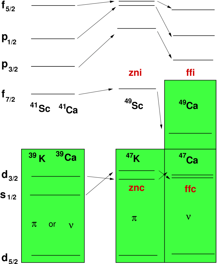
Figure 3: Evolution of $cs\pm 1$ states from ⁴⁰Ca to ⁴⁸Ca

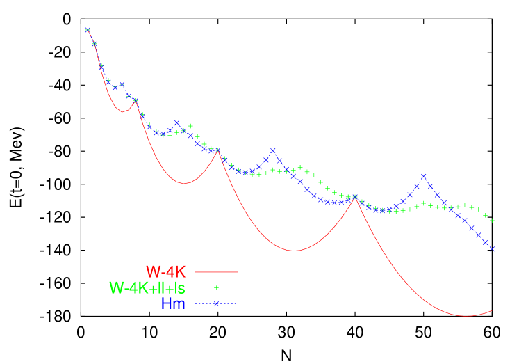
Figure 4: The different contributions to $\tilde{\cal H}^{d}_{m}$ for N=Z nuclei

[II] $\hat{\Omega}(ls)\approx-22\,l\cdot s/A^{2/3}$ (very much the value in (Bohr and Mottelson, 1969, Eq. (2-132)) and $\hat{\Omega}(ll)\approx-22[l(l+1)-p(p+3)/2]/A^{2/3}$ (in MeV), are $\hat{\Omega}$-type operators that reproduce the single-particle spectra above HO closed shells.

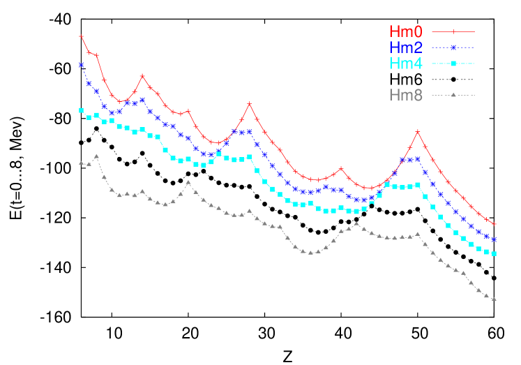
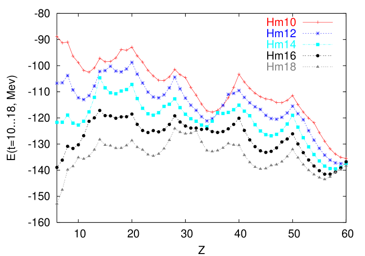
Figure 5: $\tilde{\cal H}^{d}_{m}$ for even $t=N-Z=10\ldots 18$.

[III] $\hat{\Omega}(ffi)$, $\hat{\Omega}(zni)$, $\hat{\Omega}(ffc)$ and $\hat{\Omega}(znc)$ are $\hat{\Omega}$-type 2b operators whose effect is illustrated in Fig. 3: In going from ⁴⁰Ca to ⁴⁸Ca the filling of the $f_{7/2}$ ($f$ for short) neutron orbit modifies the spectra in ⁴⁹Ca, ⁴⁹Sc, ⁴⁷Ca and ⁴⁷K.

As mentioned, realistic 2b forces will miss the particle spectrum in ⁴¹Ca. Once it is phenomenologically corrected by $ls+ll$ such forces account reasonably well for the $zni$ and $eei$ mechanism, within one major exception: they fail to depress the $f_{7/2}$ orbit with respect to the others. As a consequence, and quite generally, they fail to produce the EI closures. Though $zni$ and $eei$ can be made to cure this serious defect, it is not clear how well they do it, since the correct mechanism necessarily involves 3b terms, as will be demonstrated in Section V.1. Another problem that demands a three body mechanism is associated with the $znc$ and $ffc$ operators which always depress orbits of larger $l$ [as in the hole spectra of ⁴⁷Ca and ⁴⁷K in Fig. 3], which is not the case for light nuclei as seen from the spectra of ¹³C and ²⁹Si. Only 3b operators can account for this inversion.

In spite of these caveats, $\tilde{\cal H}_{m}^{d}$ should provide a plausible view of shell formation, illustrated in Figure 4 for $t=N-Z=0$ nuclei. $\tilde{\cal H}_{m}^{d}$ is calculated by filling the oscillator orbits in the order dictated by $ls+ll$. The $W-4K$ term produces enormous HO closures (showing as spikes). They are practically erased by the 1b contributions, and it takes the 2b ones to generate the EI spikes. Note that the HO magicity is strongly attenuated but persists. The drift toward smaller binding energies that goes as $A^{1/3}$ is an artifact of the $W-4K$ choice and should be ignored.

In Figs. 5 we show the situation for even $t=N-Z=0$ to 18. Plotting along lines of constant $t$ has the advantage of detecting magicity for both fluids. In other words, the spikes appear when either fluid is closed, and are reinforced when both are closed. The spikes are invariably associated either to the HO magic numbers (8, 20, 40) or to the EI ones (14, 28, 50), but the latter always show magicity while the former only do it at and above the double closures ($Z,N$)=(8,14),(20,28) and (40,50). For example, at $Z=20$ ⁴⁰Ca shows as a weak closure. ^{42, 44, 46}Ca are not closed (which agrees with experiment), ⁴⁸Ca is definitely magic, and spikes persist for the heavier isotopes. At $Z=40$, ⁸⁰Zr shows a nice spike, a bad prediction for a strongly rotational nucleus. However, there are no (or weak) spikes for the heavier isotopes except at ⁹⁰Zr and ⁹⁶Zr, both definitely doubly magic. There are many other interesting cases, and the general trend is the following: No known closure fails to be detected. Conversely, not all predicted closures are real. They may be erased by deformation—as in the case of ⁸⁰Zr—but this seldom happens, thus suggesting fairly reliable predictive power for $\tilde{\cal H}^{d}_{m}$.

II.3 The multipole Hamiltonian

The multipole Hamiltonian is defined as ${\cal H}_{M}$=${\cal H}$-${\cal H}_{m}$. As we are no longer interested in the full ${\cal H}$, but its restriction to a finite space, ${\cal H}_{M}$ will be more modestly called $H_{M}$, with monopole-free matrix elements given by

$$W_{rstu}^{JT}=V_{rstu}^{JT}-\delta_{rs}\delta_{tu}V_{rs}^{T}.$$ (27)

We shall describe succinctly the main results of Dufour and Zuker (1996), insisting on points that were not stressed sufficiently in that paper (Section II.3.1), and adding some new information (Section II.4).

There are two standard ways of writing $H_{M}$:

$$H_{M}=\sum\limits_{r\leq s,t\leq u,\Gamma}W_{rstu}^{\Gamma}Z_{rs\Gamma}^{\dagger}\cdot Z_{tu\Gamma},\quad{\rm or}$$ (28)

$$H_{M}=\sum_{rstu\Gamma}[\gamma]^{1/2}f_{rtsu}^{\gamma}(S_{rt}^{\gamma}S_{su}^{\gamma})^{0},$$ (29)

where $f_{rtsu}^{\gamma}=\omega_{rtsu}^{\gamma}\sqrt{(1+\delta_{rs})(1+\delta_{tu})}/4$. The matrix elements $\omega_{rtsu}^{\gamma}$ and $W_{rstu}^{\Gamma}$ are related through Eqs. (107) and (108).

Replacing pairs by single indices $rs\equiv x$, $tu\equiv y$ in eq. (28) and $rt\equiv a$, $su\equiv b$ in eq. (29), we proceed as in Eqs. (14) and (15) to bring the matrices $W_{xy}^{\Gamma}\equiv W_{rstu}^{\Gamma}$ and $f_{ab}^{\gamma}\equiv f_{rtsu}^{\gamma}$, to diagonal form through unitary transformations $U_{xk}^{\Gamma},u_{ak}^{\gamma}$ to obtain factorable expressions

$$H_{M}=\sum_{k,\Gamma}E_{k}^{\Gamma}\sum_{x}U_{xk}^{\Gamma}Z_{x\Gamma}^{\dagger}\cdot\sum\limits_{y}U_{yk}^{\Gamma}Z_{y\Gamma},$$ (30)

$$H_{M}=\sum_{k,\gamma}e_{k}^{\gamma}\left(\sum_{a}u_{ak}^{\gamma}S_{a}^{\gamma}\sum_{b}u_{bk}^{\gamma}S_{b}^{\gamma}\right)^{0}[\gamma]^{1/2},$$ (31)

which we call the $E$ (or normal or particle-particle or pp) and $e$ (or multipole or particle-hole or ph) representations. Since ${\cal H}_{m}$ contains all the $\gamma=00$ and 01 terms, for ${\cal H}_{M}$, $\omega_{rstu}^{00}=\omega_{rstu}^{01}=0$ (see Eq. (120). There are no one body contractions in the $e$ representation because they are all proportional to $\omega_{rstu}^{0\tau}$.

The eigensolutions in eqs. (30) and (31) using the KLS interaction Kahana et al. (1969b); Lee (1969), yield the density of eigenvalues (their number in a given interval) in the $E$ representation that is shown in Fig. 6 for a typical two-shell case.

Figure 6: $E$-eigenvalue density for the KLS interaction in the pf+sdg major shells $\hbar\omega=9$. Each eigenvalue has multiplicity $[\Gamma]$. The largest ones are shown by arrows.

It is skewed, with a tail at negative energies which is what we expect from an attractive interaction.

Figure 7: $e$-eigenvalue density for the KLS interaction in the pf+sdg major shells. Each eigenvalue has multiplicity $[\gamma]$. The largest ones are shown by arrows.

The $e$ eigenvalues are plotted in fig. 7. They are very symmetrically distributed around a narrow central group, but a few of them are neatly detached. The strongest have $\gamma^{\pi}=1^{-}0,\;1^{+}1,~{}2^{+}0,~{}3^{-}0,~{}4^{+}0$. “If the corresponding eigenvectors are eliminated from H in” eq. (31) and the associated H in eq. (30) is recalculated, the E distribution becomes quite symmetric, as expected for a random interaction.

If the diagonalizations are restricted to one major shell, negative parity peaks are absent, but for the positive parity ones the results are practically identical to those of Figs. 6 and 7, except that the energies are halved. This point is crucial:

If $u_{p_{1}}$ and $u_{p_{2}}$ are the eigenvectors obtained in shells $p_{1}$ and $p_{2}$, their eigenvalues are approximately equal $e_{p_{1}}\approx e_{p_{2}}=e$. When diagonalizing in $p_{1}+p_{2}$, the unnormalized eigenvector turns out to be $u_{p_{1}}+u_{p_{2}}$ with eigenvalue $e$.

In the figures the eigenvalues for the two shell case are doubled, because they are associated with normalized eigenvectors. To make a long story short: The contribution to $H_{M}$ associated to the large $\Gamma=01$, and $\gamma=20$ terms,

$$H_{\bar{P}} = -\frac{\hbar\omega}{\hbar\omega_{0}}{|E^{01}|}(\overline{P}\,^{\dagger}_{p}+\overline{P}\,^{\dagger}_{p+1})\cdot(\overline{P}_{p}+\overline{P}_{p+1})$$ (32)

$$H_{\bar{q}} = -\frac{\hbar\omega}{\hbar\omega_{0}}{|e^{20}|}(\bar{q}_{p}+\bar{q}_{p+1})\cdot(\bar{q}_{p}+\bar{q}_{p+1}),$$ (33)

turns out to be the usual pairing plus quadrupole Hamiltonians, except that the operators for each major shell of principal quantum number $p$ are affected by a normalization. $E^{01}$ and $e^{20}$ are the one shell values called generically $e$ in the discussion above. To be precise

$$\bar{P}^{\dagger}_{p}=\sum\limits_{r\in p}Z_{rr01}^{\dagger}\Omega_{r}^{1/2}/\Omega_{p}^{1/2},$$ (34)

$$\bar{q}_{p}=\sum\limits_{rs\in p}S_{rs}^{20}q_{rs}/{\cal N}_{p},$$ (35)

$${\rm where}\quad\Omega_{r}=j_{r}+1,\quad q_{rs}=\sqrt{\frac{1}{5}}\langle r\|r^{2}Y^{2}\|s\rangle$$ (36)

$${\rm and}\quad\Omega_{p}=\frac{1}{2}D_{p},\quad{\cal N}_{p}^{2}=\Sigma q_{rs}^{2}\cong\frac{5}{32\pi}(p+3/2)^{4}$$ (37)

II.3.1 Collapse avoided

The pairing plus quadrupole ($P+Q$) model has a long and glorious history Baranger and Kumar (1968); Bes and Sorensen (1969), and one big problem: as more shells are added to a space, the energy grows, eventually leading to collapse. The only solution was to stay within limited spaces, but then the coupling constants had to be readjusted on a case by case basis. The normalized versions of the operators presented above are affected by universal coupling constants that do not change with the number of shells. Knowing that $\hbar\omega_{0}=9$ MeV, they are $|E^{01}|/{\hbar\omega_{0}}=g^{\prime}=0.32$ and $|e^{20}|/{\hbar\omega_{0}}=\kappa^{\prime}=0.216$ in Eqs. (32) and (33).

Introducing $A_{mf}\approx\frac{2}{3}(p_{f}+3/2)^{3}$, the total number of particles at the middle of the Fermi shell $p_{f}$, the relationship between $g^{\prime}$, $\kappa^{\prime}$, and their conventional counterparts Baranger and Kumar (1968) is, for one shell

$$\frac{0.32\hbar\omega}{\Omega_{p}} \cong \frac{19.51}{A^{1/3}A_{mf}^{2/3}}=G\equiv{G_{0}}A^{-1},$$

$$\frac{0.216\hbar\omega}{{\cal N}_{p}^{2}} \cong \frac{1}{2}\,\frac{216}{A^{1/3}A_{mf}^{4/3}}=\frac{\chi^{\prime}}{2}\equiv\frac{\chi_{0}^{\prime}}{2}A^{-5/3}.$$ (38)

To see how collapse occurs assume $m=O(D_{f})=O(A^{2/3})$ in the Fermi shell, and promote them to a higher shell of degeneracy $D$. The corresponding pairing and quadrupole energies can be estimated as

$$E_{P}=-{|G|}{4}m(D-m+2)=-|G|O(mD),$$ (39)

$${\rm and}\quad E_{q}\approx-|\chi^{\prime}|Q_{0}^{2}=-|\chi^{\prime}|O(m^{2}D),$$ (40)

respectively, which become for the two possible scalings

$$E_{P}({\rm old})=O(\frac{mD}{A})\Longrightarrow E_{P}({\rm new})=O(\frac{m}{A^{1/3}})$$ (41)

$$E_{q}({\rm old})=O(\frac{m^{2}D}{A^{5/3}})\Longrightarrow E_{q}({\rm new})=O(\frac{m^{2}}{A^{1/3}D}).$$ (42)

If the $m$ particles stay at the Fermi shell, all energies go as $A^{1/3}$ as they should. If $D$ grows both energies grow in the old version. For sufficiently large $D$ the gain will become larger than the monopole loss $O(mD^{1/2}\hbar\omega)=O(D^{1/2}A^{1/3})$. Therefore the traditional forces lead the system to collapse. In the new form there is no collapse: $E_{P}$ stays constant, $E_{q}$ decreases and the monopole term provides the restoring force that guarantees that particles will remain predominantly in the Fermi shell.

As a model for ${\cal H}_{M}$, $P+Q$ is likely to be a reasonable first approximation for many studies, provided it is supplemented by a reasonable ${\cal H}_{m}$, to produce the $P+Q+m$ model.

II.4 Universality of the realistic interactions

To compare sets of matrix elements we define the overlaps

$$O_{AB}=V_{A}\cdot V_{B}=\sum_{rstu\Gamma}V^{\Gamma}_{rstuA}V^{\Gamma}_{rstuB}$$ (43)

$$\overline{O}_{AB}=\frac{O_{AB}}{\sqrt{O_{AA}O_{BB}}}.$$ (44)

Similarly, $O_{AB}^{T}$ is the overlap for matrix elements with the same $T$. $O_{AA}$ is a measure of the strength of an interaction. If the interaction is referred to its centroid (and a fortiori if it is monopole-free), $O_{AA}\equiv\sigma^{2}_{A}$.

Table 1: The overlaps between the KLS($A$) and Bonn($B$) interactions for the first ten oscillator shells (2308 matrix elements), followed by those for the $pf$ shell (195 matrix elements) for the BonnC ($C$) and KB ($K$) interactions.

$O_{AA}^{0}=17.56$		$O_{AA}^{1}=2.61$		$O_{AA}=6.49$
$O_{BB}^{0}=11.84$		$O_{BB}^{1}=2.31$		$O_{BB}=4.78$
$\overline{O}_{AB}^{0}=\ 0.98$		$\overline{O}_{AB}^{1}=0.99$		$\overline{O}_{AB}=0.98$
$O_{CC}^{0}=\ 3.71$		$O_{CC}^{1}=0.56$		$O_{CC}=1.41$
$O_{KK}^{0}=\ 3.02$		$O_{KK}^{1}=0.46$		$O_{KK}=1.15$
$\overline{O}_{CK}^{0}=\ 0.99$		$\overline{O}_{CK}^{1}=0.97$		$\overline{O}_{CK}=0.99$

The upper set of numbers in Table 1 contains what is probably the most important single result concerning the interactions: a 1969 realistic potential (Kahana et al. (1969b); Lee (1969)) and a modern Bonn one Hjorth-Jensen (1996) differ in total strength(s) but the normalized $\overline{O}(AB)$ are very close to unity.

Now: all the modern realistic potentials agree closely with one another in their predictions except for the binding energies. For nuclear matter the differences are substantial Pieper et al. (2001), and for the BonnA,B,C potentials studied by Hjorth-Jensen et al. (1995), they become enormous. However, the matrix elements given in this reference for the $pf$ shell have normalized cross overlaps of better than 0.998. At the moment, the overall strengths must be viewed as free parameters.

At a fundamental level the discrepancies in total strength stem for the degree of non-locality in the potentials and the treatment of the tensor force. In the old interactions, uncertainties were also due to the starting energies and the renormalization processes, which, again, affect mainly the total strength(s), as can be gathered from the bottom part of Table 1.

The dominant terms of $H_{M}$ are central and table 2 collects their strengths (in MeV) for effective interactions in the $pf$-shell: Kuo and Brown (1968) (KB), the potential fit of Richter et al. (1991) (FPD6), the Gogny force—successfully used in countless mean field studies— Dechargé and Gogny (1980) and BonnC Hjorth-Jensen et al. (1995).

There is not much to choose between the different forces which is a nice indication that overall nuclear data (used in the FPD6 and Gogny fits) are consistent with the $NN$ data used in the realistic KB and BonnC G-matrices. The splendid performance of Gogny deserves further study. The only qualm is with the weak quadrupole strength of KB, which can be understood by looking again at the bottom part of Table 1. In assessing the $JT=01$ and $JT=10$ pairing terms, it should be borne in mind that their renormalization remains an open question Dufour and Zuker (1996).

Conclusion: Some fine tuning may be in order and 3b forces may (one day) bring some multipole news, but as of now the problem is ${\cal H}_{m}$, not ${\cal H}_{M}$.

Table 2: Leading terms of the multipole Hamiltonian

Interaction	particle-particle		particle-hole
	JT=01	JT=10	$\lambda\tau$=20	$\lambda\tau$=40	$\lambda\tau$=11
KB	-4.75	-4.46	-2.79	-1.39	+2.46
FPD6	-5.06	-5.08	-3.11	-1.67	+3.17
GOGNY	-4.07	-5.74	-3.23	-1.77	+2.46
BonnC	-4.20	-5.60	-3.33	-1.29	+2.70

III The solution of the secular problem in a finite space

Once the interaction and the valence space ready, it is time to construct and diagonalize the many body secular matrix of the Hamiltonian describing the (effective) interaction between valence particles in the valence space. Two questions need now consideration: which basis to take to calculate the non-zero many-body matrix elements (NZME) and which method to use for the diagonalization of the matrix.

III.1 The Lanczos method

Figure 8: $m$-scheme dimensions and total number of non-zero matrix elements in the $pf$-shell for nuclei with $M=T_{z}=0$

In the standard diagonalization methods Wilkinson (1965) the CPU time increases as $N^{3}$, $N$ being the dimension of the matrix. Therefore, they cannot be used in large scale shell model (SM) calculations. Nuclear SM calculations have two specific features. The first one is that, in the vast majority of the cases, only a few (and very often only one) eigenstates of a given angular momentum ($J$) and isospin ($T$) are needed. Secondly, the matrices are very sparse. As can be seen in figure 8, the number of NZME varies linearly instead of quadratically with the size of the matrices. For these reasons, iterative methods are of general use, in particular the Lanczos method Lanczos (1950). As an alternative, the Davidson method Davidson (1975) has the advantage of avoiding the storage of a large number of vectors, however, the large increase in storage capacity of modern computers has somehow minimized these advantages.

The Lanczos method consists in the construction of an orthogonal basis in which the Hamiltonian matrix ($H$) is tridiagonal.

A normalized starting vector (the pivot) $|1\rangle$ is chosen. The vector $|a_{1}\rangle=H|1\rangle$ has necessarily the form

$$|a_{1}\rangle=H_{11}|1\rangle+|2^{\prime}\rangle,\quad{\rm with\ }\langle 1|2^{\prime}\rangle=0.$$ (45)

Calculate $H_{11}=\langle 1|H|1\rangle$ through $\langle 1|a_{1}\rangle=H_{11}$. Normalize $|2\rangle=|2^{\prime}\rangle/\langle 2^{\prime}|2^{\prime}\rangle^{1/2}$ to find $H_{12}=\langle 1|H|2\rangle=\langle 2^{\prime}|2^{\prime}\rangle^{1/2}$. Iterate until state $|k\rangle$ has been found. The vector $|a_{k}\rangle=H|k\rangle$ has necessarily the form

$$|a_{k}\rangle=H_{k\,k-1}|k-1\rangle+H_{k\,k}|k\rangle+|(k+1)^{\prime}\rangle.$$ (46)

Calculate $\langle k|a_{k}\rangle=H_{k\,k}$. Now $|(k+1)^{\prime}\rangle$ is known. Normalize it to find $H_{k\,k+1}=\langle(k+1)^{\prime}|(k+1)^{\prime}\rangle^{1/2}$.

The (real symmetric) matrix is diagonalized at each iteration and the iterative process continues until all the required eigenvalues are converged according to some criteria. The number of iterations depends little on the dimension of the matrix. Besides, the computing time is directly proportional to the number of NZME and for this reason it is nearly linear (instead of cubic as in the standard methods) in the dimension of the matrix. It depends on the number of iterations, which in turn depends on the number of converged states needed, and also on the choice of the starting vector.

The Lanczos method can be used also as a projection method. For example in the $m$-scheme basis, a Lanczos calculation with the operator $J^{2}$ will generate states with well defined $J$. Taking these states as starting vectors, the Lanczos procedure (with $H$) will remain inside a fixed $J$ subspace and therefore will improve the convergence properties. When only one converged state is required, it is convenient to use as pivot state the solution obtained in a previous truncated calculation. For instance, starting with a random pivot the calculation of the ground state of ⁵⁰Cr in the full $pf$ space (dimension in $m$-scheme 14,625,540 Slater determinants) needs twice more iterations than if we start with the pivot obtained as solution in a model space in which only 4 particles are allowed outside the $1f_{7/2}$ shell (dimension 1,856,720). The overlap between these two $0^{+}$ states is 0.985. When more eigenstates are needed ($n_{c}>1$), the best choice for the pivot is a linear combination of the $n_{c}$ lower states in the truncated space. Even if the Lanczos method is very efficient in the SM framework, there may be numerical problems. Mathematically the Lanczos vectors are orthogonal, however numerically this is not strictly true due to the limited floating point machine precision. Hence, small numerical precision errors can, after many iterations, produce catastrophes, in particular, the states of lowest energy may reappear many times, rendering the method inefficient. To solve this problem it is necessary to orthogonalize each new Lanczos vector to all the preceding ones. The same precision defects can produce the appearance of non expected states. For example in a $m$-scheme calculation with a $J=4$, $M=0$ pivot, when many iteration are performed, it may happen that one $J=0$ and even one $J=2$ state, lower in energy than the $J=4$ states, show up abruptly. This specific problem can be solved by projecting on $J$ each new Lanczos vector.

III.2 The choice of the basis

Given a valence space, the optimal choice of the basis is related to the physics of the particular problem to be solved. As we discuss later, depending on what states or properties we want to describe (ground state, yrast band, strength function,…) and depending on the type of nucleus (deformed, spherical,…) different choices of the basis are favored. There are essentially three possibilities depending on the underlying symmetries: $m$-scheme, $J$ coupled scheme, and $JT$ coupled scheme.

Table 3: Some dimensions in the $pf$ shell

A	4	8	12	16	20
$M=T_{z}=0$	4000	$2\times 10^{6}$	$1.10\times 10^{8}$	$1.09\times 10^{9}$	$2.29\times 10^{9}$
$J=T_{z}=0$	156	41355	$1.78\times 10^{6}$	$1.54\times 10^{7}$	$3.13\times 10^{7}$
$J=T=0$	66	9741	$3.32\times 10^{5}$	$2.58\times 10^{6}$	$5.05\times 10^{6}$

As the $m$-scheme basis consists of Slater Determinants (SD) the calculation of the NZME is trivial, since they are equal to the decoupled two body matrix element (TBME) up to a phase. This means that, independently of the size of the matrix, the number of possible values of NZME is relatively limited. However, the counterpart of the simplicity of the $m$-scheme is that only $J_{z}$ and $T_{z}$ are good quantum numbers, therefore all the possible $(J,T)$ states are contained in the basis and as a consequence the dimensions of the matrices are maximal. For a given number of valence neutrons, $n_{v}$, and protons, $z_{v}$ the number of different Slater determinants that can be built in the valence space is :

$$d=\left(\begin{array}[]{c}D_{n}\\ n_{v}\end{array}\right)\cdot\left(\begin{array}[]{c}D_{p}\\ z_{v}\end{array}\right)$$ (47)

where $D_{n}$ and $D_{p}$ are the degeneracies of the neutron and proton valence spaces. Working at fixed M and T_z the bases are smaller ($d=\sum_{M,T_{z}}d\;(M,T_{z})$). The $J$ or $JT$ coupled bases, split the full $m$-scheme matrix in boxes whose dimensions are much smaller. This is especially spectacular for the $J=T=0$ states (see table 3).

It is often convenient to truncate the space. In the particular case of the $pf$ shell, calling $f$ the largest subshell ($f_{7/2}$), and $r$, generically, any or all of the other subshells of the $p=3$ shell, the possible $t$-truncations involve the spaces

$$f^{m-m_{0}}r^{m_{0}}+f^{m-m_{0}-1}r^{m_{0}+1}+\cdots+f^{m-m_{0}-t}r^{m_{0}+t},$$ (48)

where $m_{0}\neq 0$ if more than 8 neutrons (or protons) are present. For $t=m-m_{0}$ we have the full space $(pf)^{m}$ for $A=40+m$.

In the late 60’s, the Rochester group developed the algorithms needed for an efficient work in the $(J,T)$ coupled basis and implemented them in the Oak-Ridge Rochester Multi-Shell code French et al. (1969). The structure of the calculation is as follows: In the first place, the states of $n_{i}$ particles in a given $j_{i}$ shell are defined: $|\gamma_{i}\rangle=|(j_{i})^{n_{i}}v_{i}J_{i}x_{i}\rangle$ ($v_{i}$ is the seniority and $x_{i}$ any extra quantum number). Next, the states of $N$ particles distributed in several shells are obtained by successive angular momentum couplings of the one-shell basic states:

$$\left[\left[\left[|\gamma_{1}\rangle|\gamma_{2}\rangle\right]^{\Gamma_{2}}|\gamma_{3}\rangle\right]^{\Gamma_{3}}\ldots|\gamma_{k}\rangle\right]^{\Gamma_{k}}.$$ (49)

Compared to the simplicity of the $m$-scheme, the calculation of the NZME is much more complicated. It involves products of 9j symbols and coefficients of fractional parentage (cfp), i.e., the single-shell reduced matrix elements of operators of the form

$$(a^{\dagger}_{j_{1}}a^{\dagger}_{j_{2}})^{\lambda},\;(a^{\dagger}_{j_{1}}a_{j_{2}})^{\lambda},\;a^{\dagger}_{j_{1}},\;((a^{\dagger}_{j_{1}}a^{\dagger}_{j_{2}})^{\lambda}a_{j_{3}})^{j_{4}}.$$ (50)

This complexity explains why in the OXBASH code Brown et al. (1985), the JT-coupled basis states are written in the $m$-scheme basis to calculate the NZME. The Oxford-Buenos Aires shell model code, widely distributed and used has proven to be an invaluable tool in many calculations. Another recent code that works in JT-coupled formalism is the Drexel University DUPSM Novoselsky and Vallières (1997) has had a much lesser use.

In the case of only $J$ (without $T$) coupling, a strong simplification in the calculation of the NZME can be achieved using the Quasi-Spin formalism Lawson and Macfarlane (1965); Kawarada and Arima (1964); Ichimura and Arima (1966), as in the code NATHAN described below. The advantages of the coupled scheme decrease also when $J$ and $T$ increase. As an example, in ⁵⁶Ni the ratio dim($M=J$)/dim($J$) is 70 for $J=0$ but only 5.7 for $J=6$. The coupled scheme has another disadvantage compared to the $m$-scheme. It concerns the percentage of NZME. Let us give the example of the state $4^{+}$ in ⁵⁰Ti (full $pf$ space); the percentages of NZME are respectively 14% in the $JT$-basis (see Novoselsky et al., 1997), 5% in the J-basis and only 0.05% in $m$-scheme. For all these reasons and with the present computing facilities, we can conclude that the $m$-scheme is the most efficient choice for usual SM calculations, albeit with some notable exceptions that we shall mention below.

III.3 The Glasgow $m$-scheme code

The steady and rapid increase of computer power in recent years has resulted in a dramatic increase in the dimensionality of the SM calculations. A crucial point nowadays is to know what are the limits of a given computer code, their origin and their evolution. As far as the NZME can be calculated and stored, the diagonalization with the Lanczos method is trivial. It means that the fundamental limitation of standard shell model calculations is the capacity to store the NZME. This is the origin of the term “giant” matrices, that we apply to those for which it is necessary to recalculate the NZME during the diagonalization process. The first breakthrough in the treatment of giant matrices was the SM code developed by the Glasgow group Whitehead et al. (1977). Let us recall its basic ideas: It works in the $m$-scheme and each SD is represented in the computer by an integer word. Each bit of the word is associated to a given individual state $|nljm\tau\rangle$. Each bit has the value 1 or 0 depending on whether the state is occupied or empty. A two-body operator $a^{\dagger}_{i}a^{\dagger}_{j}a_{k}a_{l}$ will select the words having the bits $i,j,k,l$ in the configuration 0011, say, and change them to 1100, generating a new word which has to be located in the list of all the words using the bi-section method.

III.4 The $m$-scheme code ANTOINE

The shell model code ANTOINE Caurier and Nowacki (1999) has retained many of these ideas, while improving upon the Glasgow code in the several aspects. To start with, it takes advantage of the fact that the dimension of the proton and neutron spaces is small compared with the full space dimension, with the obvious exception of semi-magic nuclei. For example, the 1,963,461 SD with $M=0$ in ⁴⁸Cr are generated with only the 4,865 SD (corresponding to all the possible $M$ values) in ⁴⁴Ca. The states of the basis are written as the product of two SD, one for protons and one for neutrons: $|I\rangle=|i,\alpha\rangle$. We use, $I,J,$ capital letters for states in the full space, $i,j,$ small case Latin letters for states of the first subspace (protons or neutrons), $\alpha$, $\beta$, small case Greek letters for states of the second subspace (neutrons or protons). The Slater determinants $i$ and $\alpha$ can be classified by their $M$ values, $M_{1}$ and $M_{2}$. The total $M$ being fixed, the SD’s of the 2 subspaces will be associated only if $M_{1}+M_{2}=M$. A pictorial example is given in fig. 9.

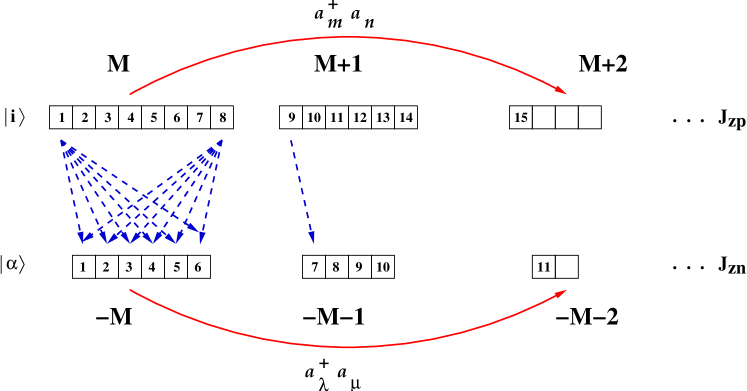
Figure 9: Schematic representation of the basis

It is clear that for each $|i\rangle$ state the allowed $|\alpha\rangle$ states run, without discontinuity, between a minimum and a maximum value. Building the basis in the total space by means of an $i$-loop and a nested $\alpha$-loop, it is possible to construct numerically an array $R(i)$ that points to the $|I\rangle$ state:

$$I=R(i)+\alpha$$ (51)

For example, according to figure 9, the numerical values of $R$ are: $R(1)=0$, $R(2)=6$, $R(3)=12$,…The relation (51) holds even in the case of truncated spaces, provided we define sub-blocks labeled with $M$ and $t$ (the truncation index defined in (48)). Before the diagonalization, all the calculations that involve only the proton or the neutron spaces separately are carried out and the results stored. For the proton-proton and neutron-neutron NZME the numerical values of $R(i),R(j),W_{ij}$ and $\alpha,\beta,W_{\alpha\beta}$, where $\langle i|H|j\rangle=W_{ij}$ and $\langle\alpha|H|\beta\rangle=W_{\alpha\beta}$, are pre-calculated and stored. Therefore, in the Lanczos procedure a simple loop on $\alpha$ and $i$ generates all the proton-proton and neutron-neutron NZME, $W_{I,J}=\langle I|H|J\rangle$. For the proton-neutron matrix elements the situation is slightly more complicated. Let’s assume that the $|i\rangle$ and $|j\rangle$ SD are connected by the one-body operator $a^{\dagger}_{q}a_{r}$ (that in the list of all possible one-body operators appears at position $p$), with $q=nljm$ and $r=n^{\prime}l^{\prime}j^{\prime}m^{\prime}$ and $m^{\prime}-m=\Delta m$. Equivalently, the $|\alpha\rangle$ and $|\beta\rangle$ SD are connected by a one-body operator whose position is denoted by $\mu$. We pre-calculate the numerical values of $R(i),R(j),p$ and $\alpha,\beta,\mu$. Conservation of the total $M$ implies that the proton operators with $\Delta m$ must be associated to the neutron operators with $-\Delta m$. Thus we could draw the equivalent to figure 9 for the proton and neutron one-body operators. In the same way as we did before for $I=R(i)+\alpha$, we can now define an index $K=Q(p)+\mu$ that labels the different two-body matrix elements (TBME). Then, we denote $V(K)$ the numerical value of the proton-neutron TBME that connects the states $|i,\alpha\rangle$ and $|j,\beta\rangle$. Once $R(i),R(j),Q(p)$ and $\alpha,\beta,\mu$ are known, the non-zero elements of the matrix in the full space are generated with three integer additions:

$$I=R(i)+\alpha,\quad J=R(j)+\beta,\quad K=Q(p)+\mu.$$ (52)

The NZME of the Hamiltonian between states $|I\rangle$ and $|J\rangle$ is then:

$$\langle I|H|J\rangle=\langle J|H|I\rangle=V(K).$$ (53)

The performance of the code is optimal when the two subspaces have comparable dimensions. It becomes less efficient for asymmetric nuclei (for semi-magic nuclei all the NZME must be stored) and for large truncated spaces. No-core calculations are typical in this respect. If we consider a $N=Z$ nucleus like ⁶Li, in a valence space that comprises up to 14$\hbar\omega$ configurations, there are 50000 Slater determinants for protons and neutrons with $M=1/2$ and $t=14$. Their respective counterparts can only have $M=-1/2$ and $t=0$ and have dimensionality 1. This situation is the same as in semi-magic nuclei.

As far as two Lanczos vectors can be stored in the RAM memory of the computer, the calculations are straightforward. Until recently this was the fundamental limitation of the SM code ANTOINE. It is now possible to overcome it dividing the Lanczos vectors in segments:

$$\Psi_{f}=\sum_{k}\Psi^{(k)}_{f}.$$ (54)

The Hamiltonian matrix is also divided in blocks so that the action of the Hamiltonian during a Lanczos iteration can be expressed as:

$$\Psi_{f}^{(k)}=\sum_{q}H^{(q,k)}\Psi^{(q)}_{i}$$ (55)

The $k$ segments correspond to specific values of $M$ (and occasionally $t$) of the first subspace. The price to pay for the increase in size is a strong reduction of performance of the code. Now, $\langle I|H|J\rangle$ and $\langle J|H|I\rangle$ are not generated simultaneously when $|I\rangle$ and $|J\rangle$ do not belong at the same $k$ segment of the vector and the amount of disk use increases. As a counterpart, it gives a natural way to parallelize the code, each processor calculating some specific $\Psi^{(k)}_{f}$. This technique allows the diagonalization of matrices with dimensions in the billion range. All the nuclei of the $pf$-shell can now be calculated without truncation. Other $m$-scheme codes have recently joined ANTOINE in the run, incorporating some of its algorithmic findings as MSHELL Mizusaki (2000) or REDSTICK Ormand and Johnson (2002).

III.5 The coupled code NATHAN.

As the mass of the nucleus increases, the possibilities of performing SM calculations become more and more limited. To give an order of magnitude the dimension of the matrix of ⁵²Fe with 6 protons and 6 neutrons in the $pf$ shell is $10^{8}$. If now we consider ¹³²Ba with also 6 protons and 6 neutron-holes in a valence space of 5 shells, four of them equivalent to the $pf$ shell plus the $1h_{11/2}$ orbit, the dimension reaches $2\times 10^{10}$. Furthermore, when many protons and neutrons are active, nuclei tend to get deformed and their description requires even larger valence spaces. For instance, to treat the deformed nuclei in the vicinity of ⁸⁰Zr, the ”normal” valence space, $2p_{3/2}$, $1f_{5/2}$, $2p_{1/2}$, $1g_{9/2}$, must be complemented with, at least, the orbit $1d_{5/2}$. This means that our span will be limited to nuclei with few particles outside closed shells (¹³⁰Xe remains an easy calculation) or to almost semi-magic, as for instance the Tellurium isotopes. These nuclei are spherical, therefore the seniority can provide a good truncation scheme. This explains the interest of a shell model code in a coupled basis and quasi-spin formalism.

In the shell model code NATHAN Caurier and Nowacki (1999) the fundamental idea of the code ANTOINE is kept, i. e. splitting the valence space in two parts and writing the full space basis as the product of states belonging to these two parts. Now, $|i\rangle$ and $|\alpha\rangle$ are states with good angular momentum. They are built with the usual techniques of the Oak-Ridge/Rochester group French et al. (1969). Each subspace is now partitioned with the labels $J_{1}$ and $J_{2}$. The only difference with the $m$-scheme is that instead of having a one-to-one association ($M_{1}+M_{2}=M$), for a given $J_{1}$ we now have all the possible $J_{2}$, $J_{min}\leq J_{2}\leq J_{max}$, with $J_{min}=|J_{0}-J_{1}|$ and $J_{max}=J_{0}+J_{1}$. The continuity between the first state with $J_{min}$ and the last with $J_{max}$ is maintained and consequently the fundamental relation $I=R(i)+\alpha$ still holds. The generation of the proton-proton and neutron-neutron NZME proceeds exactly as in $m$-scheme. For the proton-neutron NZME the one-body operators in each space can be written as $O_{p}^{\lambda}=(a^{\dagger}_{j_{1}}a_{j_{2}})^{\lambda}$. There exists a strict analogy between $\Delta m$ in $m$-scheme and $\lambda$ in the coupled scheme. Hence, we can still establish a relation $K=Q(p)+\omega$. The NZME read now:

$$\langle I|H|J\rangle=\langle J|H|I\rangle=h_{ij}\cdot h_{\alpha\beta}\cdot W(K),$$ (56)

with $h_{ij}=\langle i|O_{p}^{\lambda}|j\rangle$, $h_{\alpha\beta}=\langle\alpha|O_{\omega}^{\lambda}|\beta\rangle$, and

$$W(K)\propto V(K)\cdot\left\{\begin{array}[]{ccc}i&\alpha&J\\ j&\beta&J\\ \lambda&\lambda&0\end{array}\right\},$$ (57)

where $V(K)$ is a TBME. We need to perform –as in the $m$-scheme code– the three integer additions which generate I, J, and K, but, in addition, there are two floating point multiplications to be done, since $h_{ij}$ and $h_{\alpha\beta}$, which in $m$-scheme were just phases, are now a product of cfp’s and 9j symbols (see formula 3.10 in French et al. (1969)). Within this formalism we can introduce seniority truncations, but the problem of the semi-magic nuclei and the asymmetry between the protons and neutrons spaces remains. To overcome this difficulty in equalizing the dimension of the two subspaces we have generalized the code as to allow that one of the two subspaces contains a mixing of proton and neutron orbits. For example, for heavy Scandium or Titanium isotopes, we can include the neutron $1f_{7/2}$ orbit in the proton space. For the $N=126$ isotones we have only proton shells. We then take the $1i_{13/2}$ and $1h_{9/2}$ orbits as the first subspace, while the $2f_{7/2}$, $2f_{5/2}$, $3p_{3/2}$ and $3p_{1/2}$ form the second one. The states previously defined with $J_{p}$ and $J_{n}$ are now respectively labelled $A_{1},J_{1}$ and $A_{2},J_{2}$, $A_{1}$ and $A_{2}$ being the number of particles in each subspace. In $h_{ij}$ and $h_{\alpha\beta}$ now appear mean values of all the operators in Eq.(50)

The fact that in the coupled scheme the dimensions are smaller and that angular momentum is explicitly enforced makes it possible to perform a very large number of Lanczos iterations without storage or precision problems. This can be essential for the calculation of strength functions or when many converged states are needed, for example to describe non-yrast deformed bands. The coupled code has another important advantage. It can be perfectly parallelized without restriction on the number of processors. The typical working dimension for large matrices in NATHAN is 10⁷ (10⁹ with ANTOINE). It means that there is no problem to define as many final vectors as processors are available. The calculation of the NZME is shared between the different processors (each processor taking a piece of the Hamiltonian, $H=\sum_{k}H^{(k)}$) leading to different vectors that are added to obtain the full one:

$$\Psi^{(k)}_{f}=H^{(k)}\Psi_{i},\qquad\Psi_{f}=\sum_{k}\Psi^{(k)}_{i}.$$ (58)

III.6 No core shell model

The ab initio no-core shell model (NCSM) Navrátil et al. (2000a, b) is a method to solve the nuclear many body problem for light nuclei using realistic inter-nucleon forces. The calculations are performed using a large but finite harmonic-oscillator (HO) basis. Due to the basis truncation, it is necessary to derive an effective interaction from the underlying inter-nucleon interaction that is appropriate for the basis size employed. The effective interaction contains, in general, up to $A$-body components even if the underlying interaction had, e.g. only two-body terms. In practice, the effective interaction is derived in a sub-cluster approximation retaining just two- or three-body terms. A crucial feature of the method is that it converges to the exact solution when the basis size increases and/or the effective interaction clustering increases.

In a first phase, their applications were limited to the use of realistic two-nucleon interactions, either G-matrix-based two-body interactions Zheng et al. (1994), or derived by the Lee-Suzuki procedure Suzuki and Lee (1980) for the NCSM Navrátil and Barrett (1996). This resulted in the elimination of the purely phenomenological parameter $\Delta$ used to define G-matrix starting energy. A truly ab initio formulation of the formalism was presented by Navrátil and Barrett (1998), where convergence to the exact solutions was demonstrated for the $A=3$ system. The same was later accomplished for the $A=4$ system Navrátil and Barrett (1999), where it was also shown that a three-body effective interaction can be introduced to improve the convergence of the method. The capability to derive a three-body effective interaction and apply it in either relative-coordinate Navrátil et al. (2000) or Cartesian-coordinate formalism Navrátil and Ormand (2002) together with the ability to solve a three-nucleon system with a genuine three-nucleon force in the NCSM approach Marsden et al. (2002) now opens the possibility to include a realistic three-nucleon force in the NCSM Hamiltonian and perform calculations using two- and three-nucleon forces for the $p$-shell nuclei. Among successes of the NCSM approach was the first published result of the binding energy of ⁴He with the CD-Bonn NN potential Navrátil and Barrett (1999), the near-converged results for $A=6$ using a non-local Hamiltonian Navrátil et al. (2001), the first observation of the incorrect ground-state spin in ¹⁰B predicted by the realistic two-body nucleon-nucleon interactions Caurier et al. (2002). This last result, together with the already known problems of under-binding, confirms the need of realistic three-nucleon forces, a conclusion that also stems from the Green Function Monte Carlo calculations of Wiringa and Pieper (2002) (see also Pieper and Wiringa, 2001, for a review of the results of the Urbana-Argonne collaboration for nuclei A$\leq$10).

Recently, a new version of the shell model code ANTOINE has been developed for the NCSM applications Caurier et al. (2001b). This new code allows to perform calculations in significantly larger basis spaces and makes it possible to reach full convergence for the $A=6$ nuclei. Besides, it opens the possibility to investigate slowly converging intruder states and states with unnatural parity. The largest bases reached with this code so far are, according to the number of HO excitations, the 14$\hbar\omega$ space for ⁶Li and, according the matrix dimension, the 10$\hbar\omega$ calculations for ¹⁰C. In the latter case, the $m$-scheme matrix dimension exceeds 800 millions.

III.7 Present possibilities

The combination of advances in computer technology and in algorithms has enlarged the scope of possible SM studies. The rotational band of ²³⁸U seems to be still very far from the reach of SM calculations, but predictions for ²¹⁸U are already available. Let us list some of the present opportunities.

• No-core calculations. One of the major problems of the no-core SM is the convergence of the results with the size of the valence space; For ⁶Li we can handle excitations until 14$\hbar\omega$ and at least 8$\hbar\omega$ for all the $p$-shell nuclei.

• The $pf$-shell. This where the shell model has been most successful and exact diagonalizations are now possible throughout the region Beyond ⁵⁶Ni, as the $1f_{7/2}$ orbit becomes more and more bound, truncated calculations are close to exact, for instance, in ⁶⁰Zn Mazzocchi et al. (2001) the wave-functions are fully converged when 6p-6h excitations are included.

• The $r_{3}\;g$ valence space. We use the notation $r_{p}$ for the set of the $nlj$ orbits with $2(n-1)+l=p$ excluding the orbit with maximum total angular momentum $j=p+1/2$. This space describes nuclei in the region $28<N,Z<50$; ⁵⁶Ni is taken as inert core. Most of them are nearly spherical, and can be treated without truncations. The $\beta\beta$ decay (with and without neutrinos) of ⁷⁶Ge and ⁸²Se are a prime example. The deformed nuclei ($N\sim Z\sim 40$) are more difficult because they demand the inclusion of the $2d_{5/2}$ orbit to describe prolate states and oblate-prolate shape coexistence.

• The $pfg$ space. To enlarge the $pf$ valence space to include the $1g_{9/2}$ orbit is hopeless nowadays. Furthermore, serious center of mass spuriousness is expected in the $1f_{7/2}^{-k}1g_{9/2}^{k}$ configurations (see Appendix C). For neutron rich nuclei in the Nickel region, a tractable valence space that avoids the center of mass problem can be defined: A ⁴⁸Ca core on top of which $pf$ protons and $r_{3}\;g$ neutrons are active.

• Heavy nuclei. All the semi-magic nuclei, for instance the $N=126$ isotones, can be easily studied and the addition of few particles or holes remains tractable. Some long chains of Tellurium and Bismuth isotopes have been recently studied Caurier et al. (2003).

IV The Lanczos basis

There exists a strong connection between the Lanczos algorithm, the partition function, $Z(\beta)=\sum_{i}\langle i|\exp(-\beta{\cal H})|i\rangle$, and the evolution operator $\exp(i{\cal H}t)$. In the three cases, powers of the Hamiltonian determine the properties of the systems. The partition function can be written as $Z(\beta)=\sum_{E}\rho(E)\exp(-\beta E)$ i.e., the Laplace transform of the density of states, a quantity readily accessible once the Hamiltonian has been fully diagonalized. The evolution operator addresses more specifically the problem of evolving from a starting vector into the exact ground state. We shall discuss both questions in turn.

IV.1 Level densities

For many, shell model is still synonymous with diagonalizations, in turn synonymous with black box. One still hears questions such as: Who is interested in diagonalizing a large matrix? As an answer we propose to examine Fig. 10 showing the two point-functions that define the diagonal, $H_{ii}$, and off-diagonal elements, $H_{i\,i+1}$ in a typical Lanczos construction.

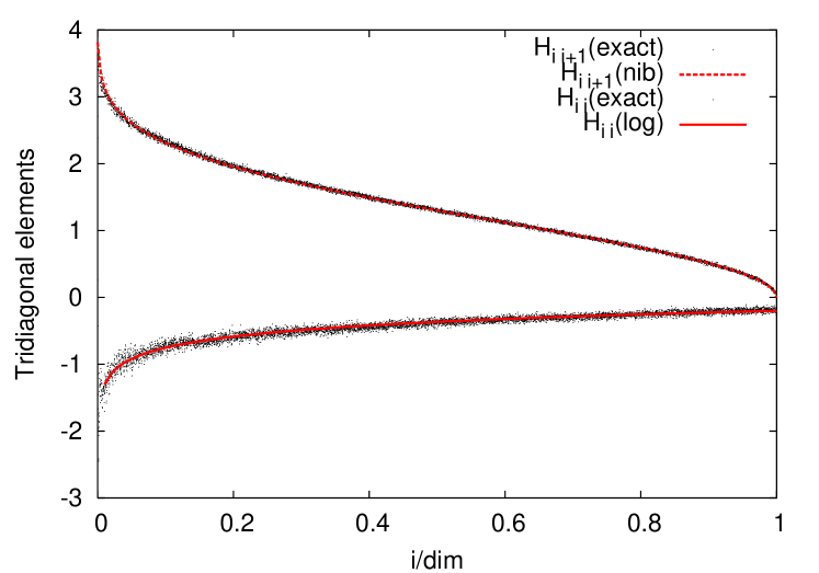
Figure 10: Tridiagonal matrix elements for a 6579 dimensional matrix, and the logarithmic and inverse binomial approximations (nib) (Zuker et al., 2001).

The continuous lines are calculated knowing the first four moments of the matrix (i.e. of the 1+2-body Hamiltonian $\mathcal{H}$ it represents). These results hold at fixed quantum numbers, i.e., when the matrix admits no block decomposition.

When the matrix is diagonalized the level density is well reproduced by a continuous binomial

$$\rho_{b}(x,N,p,S)=p^{xN}q^{\bar{x}N}d\frac{\Gamma(N+1)}{\Gamma(xN+1)\Gamma(\bar{x}N+1)}\frac{N}{S},$$ (59)

where $x$ is an a-dimensional energy, $\bar{x}=1-x$, $N$ the number of valence particles, $p$ an asymmetry parameter, $p+q=1$, and $S$ the span of the spectrum (distance between lowest and highest eigenstates). Introducing the energy scale $\varepsilon$, $S$, the centroid $E_{c}$, the variance $\sigma^{2}$ and $x$ are given by

$$S=N\varepsilon,\;E_{c}=Np\varepsilon,\;\sigma^{2}=Np(1-p)\varepsilon^{2},\;x=\frac{E}{S}.$$ (60)

Note that $\rho_{b}(x,N,p,S)$ reduces to a discrete binomial, ${N\choose n}$ if $x=n/N=n\varepsilon/S$, with integer $n$.

$N$, $p$ and $S$ are calculated using the moments of the Hamiltonian ${\cal H}$, i.e., averages given by the traces of ${\cal H}^{K}$, to be equated to the corresponding moments of $\rho_{b}(x,N,p,S)$, which for low $K$ are the same as those of a discrete binomial. The necessary definitions and equalities follow.

$$d^{-1}\text{tr}({\cal H}^{K})=\langle{\cal H}^{K}\rangle,\;E_{c}=\langle{\cal H}^{1}\rangle,\;{\cal M}_{K}=\langle({\cal H}-E_{c})^{K}\rangle$$

$$\sigma^{2}={\cal M}^{2},\quad\overline{\cal M}_{K}=\frac{{\cal M}_{K}}{\sigma^{K}},\quad\gamma_{1}=\overline{\cal M}_{3}=\frac{q-p}{\sqrt{Npq}}$$

$$\gamma_{2}=\overline{\cal M}_{4}-3=\frac{1-6pq}{Npq};\qquad d=d_{0}(1+p/q)^{N}.$$ (61)

These quantities also define the logarithmic and inverse binomial (nib) forms of $H_{ii}$ and $H_{i\,i+1}$ in Fig. 10. Note that the corresponding lines are almost impossible to distinguish from those of the exact matrix. The associated level densities are found in Fig. 11.

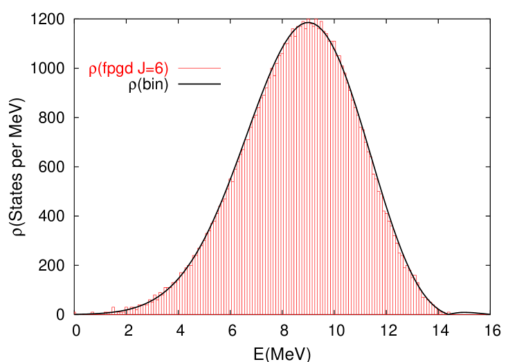
Figure 11: Exact and binomial level densities for the matrix in Fig. 10.

The mathematical status of these results is somewhat mixed. Mon and French (1975) proved that the total density of a Hamiltonian system is to a first approximation a Gaussian. Zuker (2001) extended the approximation to a binomial, but the result remains valid only in some neighborhood of the centroid. Furthermore, one does not expect it to hold generally because binomial thermodynamics is trivial and precludes the existence of phase transitions. In the example given above, we do not deal with the total density, which involves all states, $\rho=\sum_{JT}(2J+1)(2T+1)\rho_{JT}$ but with a partial $\rho_{JT}$ at fixed quantum numbers. In this case Zuker et al. (2001) conjectured that the tridiagonal elements given by the logarithmic and nib forms are valid, and hence describe the full spectrum. The conjecture breaks down if a dynamical symmetry is so strong as to define new (approximately) conserved quantum numbers.

Granted that a single binomial cannot cover all situations we may nonetheless explore its validity in nuclear physics, where the observed level densities are extremely well approximated by the classical formula of Bethe (1936) with a shift $\Delta$,

$$\rho_{B}(E,a,\Delta)=\frac{\sqrt{2\pi}}{12}\frac{e^{\sqrt{4a(E+\Delta)}}}{(4a)^{1/4}(E+\Delta)^{5/4}}.$$ (62)

Obviously, if binomials are to be useful, they must reproduce—for some range of energies—Eq. (62). They do indeed, as shown in Fig. 12, where the experimental points for ⁶⁰Ni Iljinov et al. (1992) are also given.

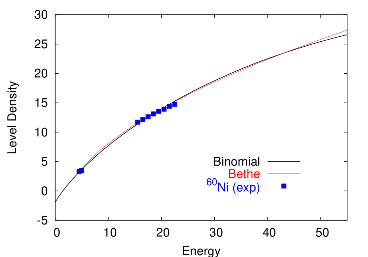
Figure 12: Binomial, Bethe and experimental level densities for ⁶⁰Ni.

Though Bethe and binomial forms are seen to be equivalent, the latter has the advantage that the necessary parameters are well defined and can be calculated, while in the former, the precise meaning of the $a$ parameter is elusive. The shift $\Delta$ is necessary to adjust the ground state position. The problem also exists for the binomial and the result in the figure Zuker (2001) solves it phenomenologically. The Shell Model Monte Carlo method provides the only parameter-free approach to level densities Dean et al. (1995); Nakada and Alhassid (1997); Langanke (1998) whose reliability is now established Alhassid et al. (1999). The problem is that the calculations are hard.

As the shape of the level density is well reproduced by a binomial except in the neighborhood of the ground state, to reconcile simplicity with full rigor we have to examine the tridiagonal matrix at the origin.

IV.2 The ground state

Obviously, some dependence on the pivot should exist. We examine it through the $J=1\,T=3$ $pf$ states in ⁴⁸Sc. The matrix is 8590-dimensional, and we calculate the ground state with two pivots, one random (homogeneous sum of all basic states), the other variational (lowest eigenstate in $f_{7/2}^{8}$ space). A zoom on the first matrix elements in Fig. 13 reveals that they are very different for the first few iterations, but soon they merge into the canonical patterns discussed in the preceding section.

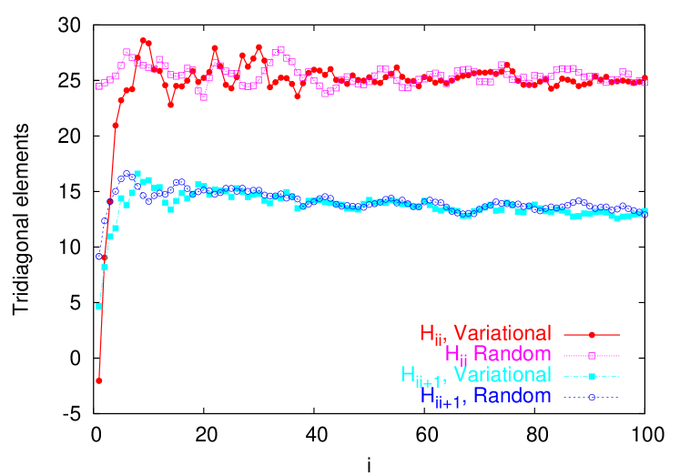
Figure 13: Tridiagonal matrix elements after 100 iterations for a random and a variational pivot.

The ground state wavefunction is unique of course, but it takes the different aspects shown in Fig. 14. In both cases the convergence is very fast, and it is not difficult to show in general that it occurs for a number of iterations of order $N\log N$ for dimensionality $d=2^{N}$. However, the variational pivot is clearly better if we are interested in the ground state: If its overlap with the exact solution exceeds 50%, all other contributions are bound to be smaller and in general they will decrease uniformly. We shall see how to exploit this property of good pivots to simplify the calculations.

IV.2.1 The exp(S) method

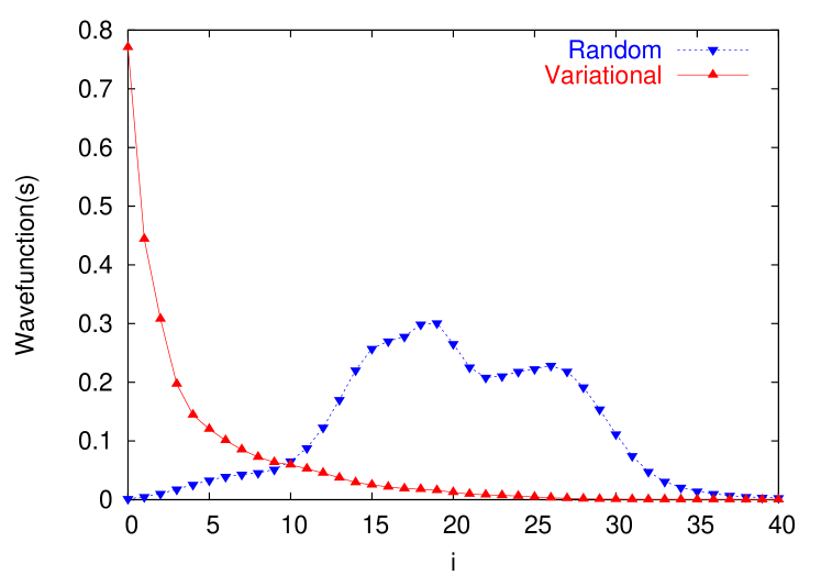
Figure 14: The ground state wavefunction in the Lanczos basis for a random, and a variational pivot. The plotted values are the squared overlaps of the successive Lanczos vectors with the final wave-function

In Section II.1.1 we have sketched the coupled-cluster (or ${\exp(S)}$) formalism. The formulation in the Lanczos basis cannot do justice to the general theory, but it is a good introduction to the underlying ideas. Furthermore, it turns out to be quite useful.

The construction is as in Eqs. (45,46), but the succeeding vectors—except the pivot—are not normalized. Then, the full wavefunction takes the form

$$|\bar{0}\rangle=(1+c_{1}P_{1}+c_{2}P_{2}+\cdots+c_{I}P_{I})|0\rangle,$$ (63)

where $P_{m}$ is a polynomial in $H$ that acting on the pivot produces orthogonal unnormalized vectors in the Lanczos basis: $P_{m}|0\rangle=|m\rangle$. Eq. (46) becomes

$${\cal H}|m\rangle=V_{m}|m-1\rangle+E_{m}|m\rangle+|m+1\rangle.$$ (64)

To relate with the normalized version ($m\Rightarrow\bar{m}$); Divide by $\langle m|m\rangle^{1/2}$, then multiply and divide $|m-1\rangle$ and $|m+1\rangle$ by their norms to recover Eq. (46), and obtain $E_{m}=H_{\bar{m}\,\bar{m}}$, $V_{m}=\langle m|m\rangle/\langle m-1|m-1\rangle=H_{\bar{m}\,\bar{m}-1}^{2}$. The secular equation $({\cal H}-E)|\bar{0}\rangle=0$ leads to the recursion

$$c_{m-1}+(E_{m}-E)\,c_{m}+V_{m+1}\,c_{m+1}=0,$$ (65)

whose solution is equivalent to diagonalizing a matrix with $V_{m+1}$ in the upper diagonal and 1 in the lower one, which is of course equivalent to the symmetric problem. However, here we shall solve the recursion by transforming it into a set of non-linear coupled equations for the $c_{m}$ amplitudes. The profound reason for using an unnormalized basis is that first term in Eq. (65), $E=E_{0}+V_{1}c_{1}$ implies that once $c_{1}$ is known the problem is solved. Calling $\varepsilon_{m}=E_{m}-E_{0}$ and replacing $E=E_{0}+V_{1}c_{1}$ in Eq (65) leads to

$$c_{m-1}+(\varepsilon_{m}-V_{1}c_{1})\,c_{m}+V_{m+1}\,c_{m+1}=0.$$ (66)

Now introduce

$$\sum c_{m}P_{m}=\exp(\sum S_{m}P_{m}),$$ (67)

Expanding the exponential and equating terms

$$c_{1} =S_{1},\quad c_{2}=S_{2}+\frac{1}{2}S_{1}^{2},$$ (68)

$$c_{3} =S_{3}+S_{1}S_{2}+\frac{1}{3!}S_{1}^{3},\;\;{\rm etc}.$$ (69)

Note that we have used the formal identification $P_{m}\,P_{n}=P_{n+m}$ as a heuristic way of suggesting Eqs. (68). Inserting in Eq. (66) and regrouping, a system of coupled equations obtains. The first two are

$$0= S_{2}V_{2}+S_{1}^{2}(\frac{1}{2}V_{2}-V_{1})+S_{1}\varepsilon_{1}+1$$ (70)

$$0= S_{3}V_{3}+S_{2}\varepsilon_{2}+S_{1}S_{2}(V_{3}-V_{1})+$$

$$\frac{1}{2}S_{1}^{2}\varepsilon_{2}+S_{1}^{3}(\frac{1}{3!}V_{3}-\frac{1}{2}V_{1})+S_{1}.$$ (71)

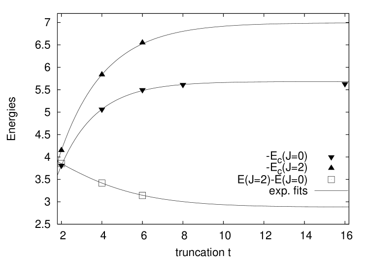
Figure 15: Energy convergence for ground and first excited state in ⁵⁶Ni as a function of the truncation level $t$ Caurier et al. (1999c).

Hence, instead of the usual $c_{m}$-truncations we can use $S_{m}$-truncations, which have the advantage of providing a model for the wavefunction over the full basis. At the first iteration Eq. (70) is solved neglecting $S_{2}$. The resulting value for $S_{1}$ is inserted in Eq. (71) which is solved by neglecting $S_{3}$. The resulting value for $S_{2}$ is reinserted in Eq. (70) and the process is repeated. Once $S_{1}$ and $S_{2}$ are known, the equation for $S_{3}$ (not shown) may be incorporated, and so on. Since the energy depends only on $S_{1}$, convergence is reached when its value remains constant from step to step. With a very good pivot, Eq. (70) should give a fair approximation, improved by incorporating Eq. (71), and checked by the equation for $S_{3}$.

If all amplitudes except $S_{1}$ are neglected, the difference scheme (65) is the same that would be obtained for an harmonic ${\cal H}\equiv\varepsilon S^{0}+V(S^{+}+S_{-})$. Successive approximations amount to introduce anharmonicities. An equivalent approach—numerically expedient—consists in diagonalizing the matrices at each $c_{m}$ truncation level. Then, after some iteration, the energies converge exponentially: Introduce

$$\text{conv}(i,a,e_{0},i_{0})=e_{0}\frac{\exp(-ai)-1}{\exp(-ai_{0})-1},$$ (72)

which equals $e_{0}$ at point $i=i_{0}$. Choose $a$ so as to yield conv$(i=i_{0}+1)=e(i_{0}+1)$ i.e., the correct energy at the next point . Check that $e(i_{0}+2)$ is well reproduced. Fig. 15 provides an example of the efficiency of the method for the lowest two states in ⁵⁶Ni. The index $i$ is replaced by the truncation level $i\equiv t/2$ [Eq. (48, with $m=16,\,m_{0}=0$]: We set $i_{0}=1$, fix $a$ so as to reproduce the energy at the second iteration and check that the curve gives indeed the correct value at the third point. The results reproduce those of the $S_{2}$ truncation, confirming that “exponential convergence” and $\exp(S)$ are very much the same thing. In this example, the closed shell pivot is particularly good, and the exponential regime sets in at the first iteration. In general, it will always set in for some value of $i_{0}$ that may be quite large (Fig. 14 suggests $i_{0}\approx 25$ for the random pivot). Fortunately, it is almost always possible to find good pivots, and the subject deserves a comment.

In the case of ⁵⁶Ni the good pivot is a closed shell. As a consequence, the first iterations are associated to truncated spaces of much smaller dimensionalities than the total one ($d_{m}\approx 10^{9}$). This also happens for lighter $pf$ shell nuclei, for which the $f_{7/2}^{m}$ [or eventually $(f_{7/2}p_{3/2})^{m}$] subspaces provide a good pivot. The same argument applies for other regions. For well deformed nuclei Hartree Fock should provide good determinantal pivots, and hence enormous gains in dimensionality, once projection to good angular momentum can be tackled efficiently.

As we shall see next, the Lanczos and $\exp S$ procedures provide a convenient framework in which to analyze other approaches.

IV.2.2 Other numerical approximation methods

The exponential convergence method introduced in the previous section was first described by Horoi et al. (1999), under a different but equivalent guise. In later work, a hierarchy of configurations determined by their average energy and width was proposed. Successive diagonalizations make it possible to reach the exact energy by exponential extrapolation. The method has been successfully applied to the calculation of the binding energies of the $pf$ shell nuclei Horoi et al. (2002) and to calculation of the excitation energies of the deformed 0⁺ states of ⁵⁶Ni and ⁵²Cr Horoi et al. (2003).

The work of Mizusaki and Imada (2002, 2003), is based on the fact that the width of the total Hamiltonian in a truncated space tends to zero as the solution approaches the exact one. They have devised different extrapolation methods and applied them to some $pf$-shell nuclei.

Andreozzi, Lo Iudice, and Porrino (2003) have recently proposed a factorization method that allows for importance sampling to approximate the exact eigenvalues and transition matrix elements.

A totally different approach which has proven its power in other fields, the density matrix renormalization group, has been proposed (Dukelsky and Pittel, 2001; Dukelsky et al., 2002), and Papenbrock and Dean (2003) have developed a method based in the optimization of product wavefunctions of protons and neutrons that seems very promising.

Still, to our knowledge, the only prediction for a truly large matrix that has preceded the exact calculation remains that of ⁵⁶Ni, $J=2$ in Fig. 15. It was borne out when the diagonalization became feasible two years later.

IV.2.3 Monte Carlo methods

Monte Carlo methods rely on the possibility to deal with the imaginary-time evolution operator acting on some trial wavefunction $\exp(-\beta{\cal H})|0\rangle$ which tends to the exact ground state $|\bar{0}\rangle$ as $\beta\Rightarrow\infty$. This is very much what the Lanczos algorithm does, but no basis is constructed. Instead, the energy (or some observable $\hat{\Omega}$) is calculated through

$$\frac{\langle 0|e^{-\beta\mathcal{H}/2}\;\hat{\Omega}\;e^{-\beta\mathcal{H}/2}|0\rangle}{\langle 0|e^{-\beta{\cal H}}|0\rangle}\stackrel{{\scriptstyle\beta\rightarrow\infty}}{{\Longrightarrow}}\frac{\langle\bar{0}|\hat{\Omega}|\bar{0}\rangle}{\langle\bar{0}|\bar{0}\rangle}$$ (73)

which is transformed into a quotient of multidimensional integrals evaluated through Monte Carlo methods with importance sampling. A “sign problem” arises because the integrands are not definite positive, leading to enormous precision problems. The Green Function Monte Carlo studies mentioned at the beginning of Section II are conducted in coordinate space. The Shell Model Monte Carlo (SMMC) variant is formulated in Fock space, and hence directly amenable to comparisons with standard SM results (see Koonin, Dean, and Langanke, 1997a, for a review). The approach relies on the Hubbard-Stratonovich transformation, and the sign problem is circumvented either by an extrapolation method or by choosing Hamiltonians that are free of it while remaining quite realistic (e.g. pairing plus quadrupole). At present it remains the only approach that can deal with much larger valence spaces than the standard shell model. It should be understood that SMMC does not lead to detailed spectroscopy, as it only produces ground state averages, but it is very well suited for finite temperature calculations. The introduction of Monte Carlo techniques in the Lanczos construction is certainly a tempting project….

The quantum Monte Carlo diagonalization method (QMCD) of Otsuka, Honma, and Mizusaki (1998) consists in exploring the mean field structure of the valence space by means of Hartree-Fock calculations that break the symmetries of the Hamiltonian. Good quantum numbers are enforced by projection techniques Peierls and Yoccoz (1957). Then the authors borrow from SMMC to select an optimal set of basic states and the full Hamiltonian is explicitly diagonalized in this basis. More basic states are iteratively added until convergence is achieved. For a very recent review of the applications of this method see Otsuka et al. (2001b). A strong connection between mean field and shell model techniques is also at the heart of the Vampir approach Petrovici et al. (1999), Schmid (2001) and of the projected shell model (PSM) Hara and Sun (1995).

IV.3 Lanczos Strength Functions

The choice of pivot in the Lanczos tridiagonal construction is arbitrary and it can be adapted to special problems. One of the most interesting is the calculation of strength functions Whitehead (1980); Bloom (1984): If $U_{i\,j}$ is the unitary matrix that achieves diagonal form, its first column $U_{i\,0}$ gives the amplitudes of the ground state wavefunction in the tridiagonal basis while the first row $U_{0\,j}$ determines the amplitude of the pivot in the $j$-th eigenstate. $U_{0\,j}^{2}$ plotted against the eigenenergies $E_{j}$ is called the “strength function” for that pivot.

In practice, given a transition operator $\mathcal{T}$, act with it on a target state $|t\rangle$ to define a pivot $|0^{\prime}\rangle={\cal T}|t\rangle$ that exhausts the sum rule $\langle 0^{\prime}|0^{\prime}\rangle$ for ${\cal T}$. Normalize it.

Figure 16: Evolution of the Gamow-Teller strength function of ⁴⁸Ca as the number of Lanczos iterations on the doorway state increases.

Then, by definition

$$|0\rangle=\frac{{\cal T}|t\rangle}{\sqrt{\langle 0^{\prime}|0^{\prime}\rangle}}=\sum_{j}U_{0j}|j\rangle,\;{\rm whose\ moments,}$$ (74)

$$\langle 0|{\cal H}^{k}|0\rangle=\sum_{j}U_{0j}^{2}E_{j}^{k},\;{\rm are\ those\ of\ the}$$ (75)

$${\rm strength\ function\ }\;S(E)=\sum_{j}\delta(E-E_{j})U_{0j}^{2},$$ (76)

Figure 17: Strength functions convoluted with gaussians: Upper panel; 50 iterations, Bottom panel; 1000 iterations.

As the Lanczos vector $|I\rangle$ is obtained by orthogonalizing ${\cal H}^{I}|0\rangle$ to all previous Lanczos vectors $|i\rangle,\;i<I$, the tridiagonal matrix elements are linear combinations of the moments of the strength distribution. Therefore the eigensolutions of the $I\times I$ matrix define an approximate strength function $S_{I}(E)=\sum_{i=1,I}\,\delta(E-E_{i})\,\langle i|{\cal T}|0\rangle^{2}$, whose first $2I-1$ moments are the exact ones. The eigenstates act as “doorways” whose strength will be split until they become exact solutions for $I$ large enough, as illustrated in Fig. 16 that retraces the fragmentation process of the sum rule pivot; in this case a ⁴⁸Sc “doorway” obtained by applying the Gamow-Teller operator to the ⁴⁸Ca ground state. The term doorway applies to vectors that have a physical meaning but are not eigenstates. After full convergence is achieved for all states in the resonance region, the strength function has the aspect shown at the bottom of the figure. In practice, all the spikes are affected by an experimental width, and assuming a perfect calculation, the observed profile would have the aspect shown at the bottom of Fig. 17, after convoluting with gaussians of 150 keV width. The upper panel shows the result for 50 iterations, and 250 keV widths for the non converged states. The profiles become almost identical.

V The $\bm{0\hbar\omega}$ calculations

In this section we first revisit the $p$, $sd$, and $pf$ shells to explain how a 3b monopole mechanism solves problems hitherto intractable. Then we propose a sample of $pf$ shell results that will not be discussed elsewhere. Finally Gamow Teller transitions and strength functions are examined in some detail.

V.1 The monopole problem and the three-body interaction

The determinant influence of the monopole interaction was first established through the mechanism of Bansal and French (1964). Its efficiency in cross-shell calculations was further confirmed by Zamick (1965), and the success of the ZBM model (Zuker, Buck, and McGrory, 1968) is implicitly due to a monopole correction to a realistic force. Zuker (1969) identified the main shortcoming of the model as due to what must be now accepted as a 3b effect. Trouble showed in 0$\hbar\omega\,$calculations somewhat later simply because it takes larger matrices to detect it in the $sd$ shell than in the ZBM space (dimensionalities of 600 against 100 for six particles). Up to 5 particles the results of Halbert et al. (1971) with a realistic interaction were quite good, but at ²²Na they were so bad that they became the standard example of the unreliability of the realistic forces Brown and Wildenthal (1988) and lead to the titanic Universal SD (USD) fit of the 63 matrix elements in the shell by Wildenthal (1984).

Though the $pf$ shell demands much larger dimensionalities, it has the advantage of containing two doubly magic nuclei ⁴⁸Ca and ⁵⁶Ni for which truncated calculations proved sufficient to identify very early the core of the monopole problem: The failure to produce EI closures.

Figure 18: The spectrum of ⁴⁹Ca for the KB, KB’ and KB3 interactions compared to experiment

Fig. 18 gives an idea of what happens in ⁴⁹Ca with the KB interaction Kuo and Brown (1968): there are six states below 3 MeV, where only one exists. In Pasquini (1976) and Pasquini and Zuker (1978) the following modifications were proposed ($f\equiv f_{7/2},\,r\equiv f_{5/2},\,p_{3/2},\,p_{1/2}$),

$$\begin{array}[]{l}V_{fr}^{T}(\text{KB1})=V_{fr}^{T}(\text{KB})-(-)^{T}\,300\text{ keV},\\ V_{ff}^{0}(\text{KB1})=V_{ff}^{0}(\text{KB})-350\text{ keV},\\ V_{ff}^{1}(\text{KB1})=V_{ff}^{1}(\text{KB})-110\text{ keV}.\end{array}$$ (77)

The first line defines KB’ in Fig. 18. The variants KB2 and KB3 in Poves and Zuker (1981b) keep the KB1 centroids and introduce very minor multipole modifications. KB3 was adopted as standard in successful calculations in $A=47$-50 that will be described in the next sections (Caurier et al., 1994; Martínez-Pinedo et al., 1996b, 1997).

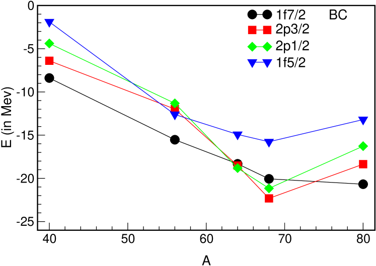
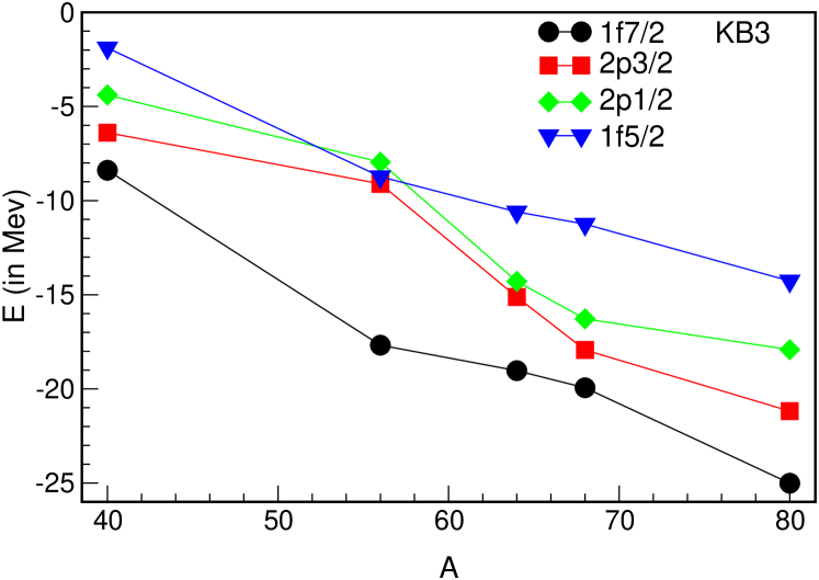
Figure 19: Effective single particle energies in the $pf$-shell along the $N=Z$ line, computed with the BC and KB3 interactions.

For higher masses, there are some problems, but nothing comparable to the serious ones encountered in the $sd$ shell, where modifications such as in Eq. (77) are beneficial but (apparently) insufficient. The effective single particle energies in Fig. 19 are just the monopole values of the particle and hole states at the subshell closures. They give an idea of what happens in a 2b description. At the origin, in ⁴¹Ca, the spectrum is the experimental one. At ⁵⁷Ni there is a bunching of the upper orbits that the realistic BonnC (BC) and KB describe reasonably well, but they fail to produce a substantial gap. Hence the need of KB1-type corrections. At the end of the shell BC and KB reproduce an expanded version of the ⁴¹Ca spectrum, which is most certainly incorrect. The indication from $\tilde{\cal H}_{m}^{d}$ in Eq. (II.2.2) is that the bunching of the upper orbits should persist. By incorporating this hint—which involves the $V_{rr^{\prime}}$ centroids—and fine-tuning the $V_{fr}$ ones Poves et al. (2001) defined a KB3G interaction that brings interesting improvements over KB3 in $A=50$-52, but around ⁵⁶Ni there are still some problems, though not as severe as the ones encountered in the $sd$ and $p$ shells. Compared to KB3, the interaction FPD6 has a better gap in ⁵⁶Ni, however, the orbit 1f_5/2 is definitely too low in ⁵⁷Ni. This produces problems with the description of Gamow-Teller processes (see Borcea et al., 2001, for a recent experimental check in the beta decay of ⁵⁶Cu).

The classic fits of Cohen and Kurath (1965) (CK) defined state of the art in the $p$ shell for a long time. As they preceded the realistic G-matrices, they also contributed to hide the fact that the latter produce in ¹⁰B a catastrophe parallel to the one in ²²Na. The work of  Navrátil and Ormand (2002), and Pieper, Varga, and Wiringa (2002) acted as a powerful reminder that brought to the fore the 3b nature of the discrepancies.

Once this is understood, the solution follows: Eq. (77) is assumed to be basically sound but the corrections are taken to be linear in the total number of valence particles $m$ (the simplest form that a 3b term can take).

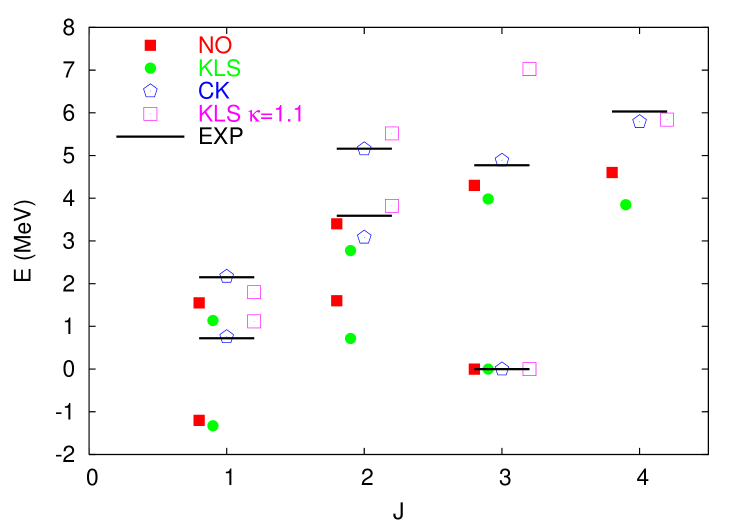
Figure 20: The excitation spectrum of ¹⁰B for different interactions.

Using $f\equiv(p_{3/2},\,d_{5/2},\,f_{7/2}$) generically in the ($p,\,sd,\,pf$) shells respectively, and $r=p_{1/2}$ and $r\equiv d_{3/2},s_{1/2}$ for the $p$ and $sd$ shells, Zuker (2003) proposes ($\kappa=\kappa_{0}+(m-m_{0})\,\kappa_{1}$)

$$\begin{array}[]{l}V_{fr}^{T}(\text{R})\Longrightarrow V_{fr}^{T}(\text{R})-(-)^{T}\,\kappa\\ V_{ff}^{T}(\text{R})\Longrightarrow V_{ff}^{T}(\text{R})-1.5\,\kappa\,\delta_{T_{0}}\end{array}$$ (78)

where R stands for any realistic 2b potential. The results for ¹⁰B are in Fig. 20. The black squares (NO) are from (Navrátil and Ormand, 2002, Fig 4, 6$\hbar\Omega$).

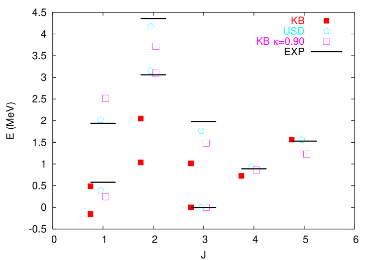
Figure 21: The excitation spectrum of ²²Na for different interactions.

The black circles correspond to the bare KLS G-matrix ($\hbar\omega\,$=17 MeV), the white squares to the same with $\kappa=1.1$, and the pentagons to the CK fit. NO and KLS give quite similar spectra, as expected from the discussion in Sections II.1 and II.4. The $\kappa$ correction eliminates the severe discrepancies with experiment and give values close to CK.

In ²²Na the story repeats itself: BC and KB are very close to one another, the ground state spin is again $J=1$ instead of $J=3$ and the whole spectrum is awful. The $\kappa$ correction restores the levels to nearly correct positions, though USD still gives a better fit. This simple cure was not discovered earlier because $\kappa$ is not a constant. In ²⁴Mg we could still do with the value for ²²Na but around ²⁸Si it must be substantially smaller. The spectra in Fig. 22 are obtained with $\kappa(m)=0.9-0.05(m-6)$, and now the spectra are as good as those given by USD.

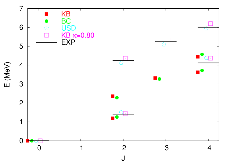
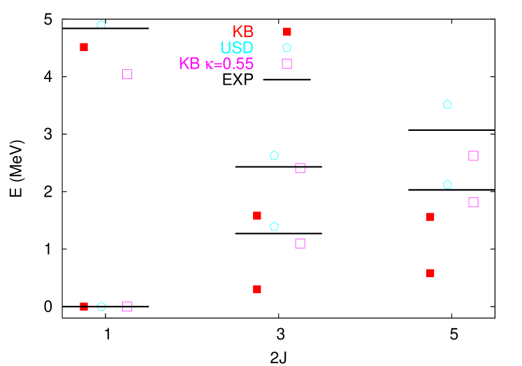
Figure 22: The excitation spectra of ²⁴Mg and ²⁹Si for different interactions.

To determine a genuine 3b effect (i.e., the linearity of $\kappa$) a sufficiently large span of $A$ values is necessary. In the $p$ shell, corrections to $V_{rr^{\prime}}$ become indispensable very soon and must be fitted simultaneously, as done successfully by Abzouzi et al. (1991), so we do not dwell on the subject. As we have seen, in the $pf$ shell KB3, which is nearly perfect in $A=47$-50, must be turned into KB3G for $A=50$-52, which also does well at the lower masses. To find a real problem with a 2b $R$-interaction (i.e., compatible with $NN$ data) we have to move to ^56,58Ni. In particular the first $B(E2)(2\longrightarrow 0)$ transition in ⁵⁸Ni falls short of the observed value (140 e²fm⁴) by a factor $\approx 0.4$ with any monopole corrected KB interaction. The problem can be traced to weak quadrupole strength and it is not serious: as explained in Section II.4 it is due to a normalization uncertainty, and Table 1 shows that with equal normalizations BC and KB in the $pf$ shell are as close as in the $sd$ shell.

In Zuker (2003) BC was adopted. Small modifications of the $V_{fr}$ matrix were made to improve the (already reasonable) $r$-spectrum in ⁵⁷Ni (see Fig. 19). The particular mixture in Eq. (78) was actually chosen to make possible, in the simplest way, a good gap in ⁴⁸Ca and a good single-particle spectrum in ⁴⁹Sc. It was found that for $A=48,\ \kappa(m=8)\approx 0.43$. For $A=56$, truncated calculations yielded $\kappa(16)\lessapprox 0.28$. The B(E2)$(2\rightarrow 0)$ in ⁵⁸Ni indicated convergence to the right value.

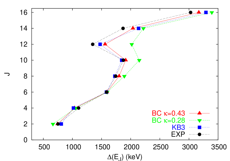
Figure 23: Backbending in ⁴⁸Cr. See text.

With $\kappa(m=8)$, BC reproduces the yrast spectrum of ⁴⁸Cr almost as well as KB3, but not with $\kappa(m=16)$ (Fig. 23), indicating that the three-body drift is needed, though not as urgently as in the $sd$ shell. Another indication comes from the T=0 spectrum of ⁴⁶V, the counterpart of ²²Na and ¹⁰B in the $pf$-shell. The realistic interactions place again the J=1 and J=3 states in the wrong order, the correct one is re-established by the three-body monopole correction.

V.2 The $pf$ shell

Systematic calculations of the A=47-52 isobars can be found in (Caurier et al., 1994, $A=48$, KB3), (Martínez-Pinedo et al., 1997, $A=47$ and 49, KB3) and (Poves et al., 2001, $A=50$-52, KB3G). Among the other full 0$\hbar\omega\,$calculations let’s highlight the following: The SMMC studies using either the FPD6 interaction Alhassid et al. (1994) or the KB3 interaction Langanke et al. (1995). A comparison of the exact results with the SMMC can be found in Caurier et al. (1999b). For a recollection of the SMMC results in the $pf$ shell see also Koonin et al. (1997b). The recent applications of the exponential extrapolation method Horoi et al. (2002, 2003). The calculations of Novoselsky et al. (1997) for ⁵¹Sc and ⁵¹Ti using the DUPSM code (see also the erratum in Novoselsky et al., 1998b) and for ⁵²Sc and ⁵²Ti Novoselsky et al. (1998a). The extensive QMCD calculation of the spectrum of ⁵⁶Ni have been able to reproduce the exact result for the ground state binding energy within 100$\sim$200 keV and to give a fairly good description of the highly deformed excited band of this doubly magic nucleus Otsuka et al. (1998); Mizusaki et al. (1999, 2002). Other applications to the $pf$ shell can be found in Honma et al. (1996). The existence of excited collective bands in the N=28 isotones is studied in Mizusaki et al. (2001). Very recently, a new interaction for the $pf$ shell (GXPF1) has been produced by a Tokyo-MSU collaboration Honma et al. (2002), following the fitting procedures that lead to the USD interaction. The fit starts with the G-matrix obtained from the Bonn-C nucleon nucleon potential Hjorth-Jensen et al. (1995). The fit privileges the upper part of the $pf$ shell, as seen by the very large difference in single particle energies between the 1f_7/2 and 12p_3/2 orbits (3 MeV instead of the standard 2 MeV). In the calcium isotopes i.e., when only the T=1 neutron neutron interaction is active) this new interaction retains the tendency of the bare G-matrices (KB, Bonn-C, KLS) to produce large gaps at N=32 and N=34, contrary to FPD6 or KB3G that only predict a large gap at N=32. Some early spectroscopic applications of GXPF1 to the heavy isotopes of Titanium, Vanadium and Chromium can be found in Janssens et al. (2002) and Mantica et al. (2003), where the N=32-34 gaps are explored.

Each nucleus has its interest, sometimes anecdotic, sometimes fundamental. The agreement with experiment for the energies, and for the quadrupole and magnetic moments and transitions is consistently good, often excellent. These results have been conclusive in establishing the soundness of the minimally-monopole-modified realistic interaction(s). There is no point in reproducing them here, and we only present a few typical examples concerning spectroscopic factors, isospin non-conserving forces and “pure spectroscopy”.

V.2.1 Spectroscopic factors

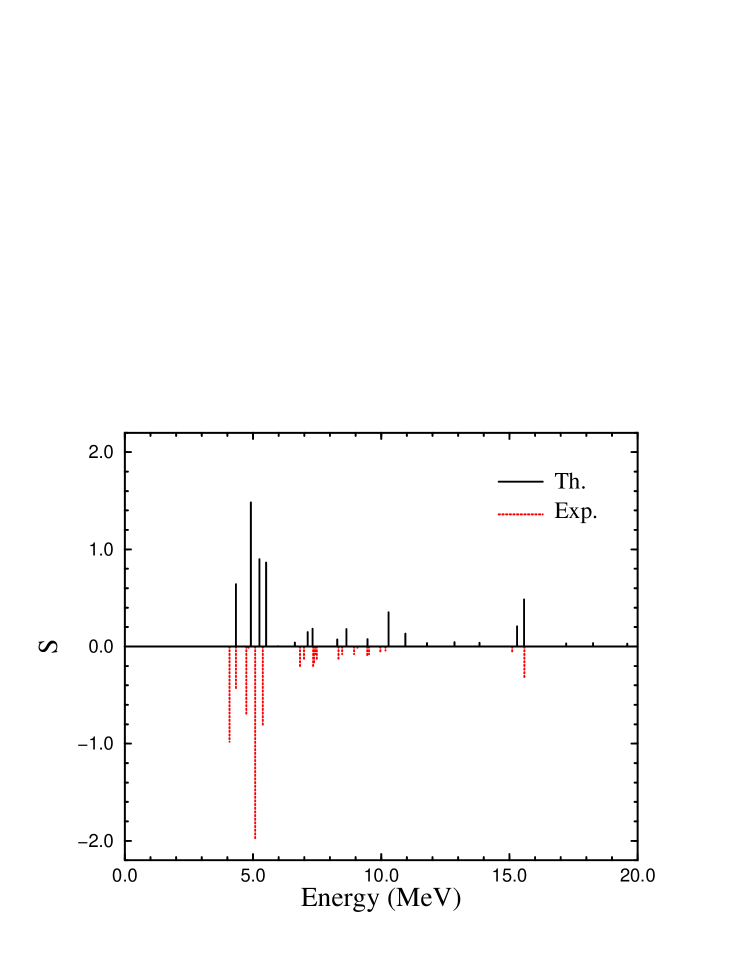
Figure 24: Spectroscopic factors, $(2j+1)S(j,t_{z})$, corresponding to stripping of a particle in the orbit 1$f_{5/2}$ Martínez-Pinedo et al. (1997).

The basic tenet of the independent particle model is that addition of a particle to a closed shell $a^{\dagger}_{r}|cs\rangle$ produces an eigenstate of the $|cs+1\rangle$ system. Nowadays we know better: it produces a doorway that will be fragmented. If we choose $|cs\rangle=|^{48}{\rm Ca}\rangle$ and $|cs+1\rangle=|^{49}{\rm Sc}\rangle$, the four $pf$ orbits provide the doorways. The lowest, $f_{7/2}$, leads to an almost pure eigenstate. The middle ones, $p_{3/2,\,1/2}$, are more fragmented, but the lowest level still has most of the strength and the fragments are scattered at higher energies. Fig. 24 shows what happens to the $f_{5/2}$ strength: it remains concentrated on the doorway but splits locally. The same evolution with energy of the quasi-particles (Landau’s term for single particle doorways) was later shown to occur generally in finite systems Altshuler et al. (1997).

V.2.2 Isospin non conserving forces

Recent experiments have identified several yrast bands in mirror $pf$ nuclei O’Leary et al. (1997); Bentley et al. (1998, 1999, 2000); O’Leary et al. (2002); Lenzi et al. (2001); Brandolini et al. (2002b) for $A=47$, 49, 50 and 51. The naive view that the Coulomb energy should account for the MDE (mirror energy differences) turns out to be untenable. The four pairs were analyzed in Zuker et al. (2002) where it was shown that three effects should be taken into account. A typical result is proposed in Fig. 25, where $V_{CM}$ and $V_{BM}$ stand for Coulomb an nuclear isospin breaking multipole contributions, while $V_{Cm}$ is a monopole Coulomb term generated by small differences of radii between the members of the yrast band. The way these disparate contributions add to reproduce the observed pattern is striking.

Figure 25: Experimental O’Leary et al. (1997) and calculated Zuker et al. (2002) MED for the pair ⁴⁹Cr-⁴⁹Mn.

Another calculation of the isospin non conserving effects, and their influence in the location of the proton drip line, is due to Ormand (1997). He has also analyzed the A=46 isospin triplet in Garrett et al. (2001).

V.2.3 Pure spectroscopy

The first nucleus we have chosen is also one that has been measured to complete the mirror band Bentley et al. (2000) in $A=51$, whose MED are as well described as those of $A=49$ in Fig. 25. Such calculations need very good wavefunctions, and the standard test they have to pass is the “purely spectroscopic” one.

Work on the subject usually starts with a litany. Such as: Quadrupole effective charges for neutrons q_ν=0.5 and protons q_π=1.5 and bare $g$-factors $g^{s}_{\pi}$=5.5857 $\mu_{N}$, $g^{s}_{\nu}$=-3.3826 $\mu_{N}$, $g^{l}_{\pi}$=1.0 $\mu_{N}$ and $g^{l}_{\nu}$=0.0 $\mu_{N}$ in $M1$ transitions and moments are used. Except when the M1 transitions are fully dominated by the spin term, the use of effective g-factors does not modify the results very much due to the compensation between the spin and orbital modifications.

Then some spectrum: The yrast band of ⁵¹Mn, calculated in the full $pf$-shell space, is compared in Fig. 26 with the experimental data. The first part of the test is passed. At most the examiner will complain about slightly too high, high spin states.

Figure 26: Yrast band of ⁵¹Mn; experiment vs shell model calculation in the full $pf$-shell space.

Finally the transitions: The transitions in Table 4 are equally satisfactory. Note the abrupt change in both $B(M1)$ and $B(E2)$ for $J=(17/2)^{-}$, beautifully reproduced by the calculation. The origin of this isomerism is in the sudden alignment of two particles in the 1f_7/2 orbit, which provides an intuitive physical explanation for the abrupt change in the MED Bentley et al. (2000).

Table 4: Transitions in ⁵¹Mn.

	Exp.	Th.
$B(M1)$	($\mu_{N}^{2}$)	($\mu_{N}^{2}$)
$\frac{7}{2}^{-}\rightarrow\frac{5}{2}^{-}$	0.207(34)	0.177
$\frac{9}{2}^{-}\rightarrow\frac{7}{2}^{-}$	0.16(5)	0.116
$\frac{11}{2}^{-}\rightarrow\frac{9}{2}^{-}$	0.662(215)	0.421
$\frac{17}{2}^{-}\rightarrow\frac{15}{2}^{-}$	0.00012(4)	0.00003
$\frac{19}{2}^{-}\rightarrow\frac{17}{2}^{-}$	$>$0.572	0.797
$B(E2)$	($e^{2}\,fm^{4}$)	($e^{2}\,fm^{4}$)
$\frac{7}{2}^{-}\rightarrow\frac{5}{2}^{-}$	528(146)	305
$\frac{9}{2}^{-}\rightarrow\frac{5}{2}^{-}$	169(67)	84
$\frac{9}{2}^{-}\rightarrow\frac{7}{2}^{-}$	303(112)	204
$\frac{11}{2}^{-}\rightarrow\frac{7}{2}^{-}$	236(67)	154
$\frac{11}{2}^{-}\rightarrow\frac{9}{2}^{-}$	232(75)	190
$\frac{17}{2}^{-}\rightarrow\frac{13}{2}^{-}$	1.236(337)	2.215

At the end one can add some extras: The electromagnetic moments of the ground state are also known: Their values $\mu_{exp}$=3.568(2)$\mu_{N}$ and Q_exp=42(7) efm² Firestone (1996) compare quite well with the calculated $\mu_{th}$=3.397$\mu_{N}$ and Q_th=35 efm².

We complete this section with an even-even and an odd-odd nucleus. In figure 27 we show the yrast states of ⁵²Cr, up to the band termination, calculated in the full $pf$-shell space. The agreement of the KB3G results with the experiment is again excellent.

Figure 27: Yrast band of ⁵²Cr; experiment $vs$ shell model calculation in the full $pf$-shell space.

Table 5: Transitions in ⁵²Cr. $(a)$ from Brown et al. (1974).

	Exp.	Th.
$B(M1)$	($\mu_{N}^{2}$)	($\mu_{N}^{2}$)
$9^{+}\rightarrow 8^{+}$	0.057(38)	0.040
$B(E2)$	($e^{2}\,fm^{4}$)	($e^{2}\,fm^{4}$)
$2^{+}\rightarrow 0^{+}$	131(6)	132
$3^{+}\rightarrow 2^{+}$	7${}^{+7}_{-5}$	5
$4^{+}_{1}\rightarrow 2^{+}$	83(17) a	107
$4^{+}_{2}\rightarrow 2^{+}$	69(19)	26
$6^{+}\rightarrow 4^{+}$	59(2)	68
$8^{+}\rightarrow 6^{+}$	75(24)	84
$9^{+}\rightarrow 8^{+}$	0.5(20)	0.6

The electromagnetic moments of the first $J=2^{+}$ state are known: $\mu_{exp}$=2.41(13) $\mu_{N}$ Speidel et al. (2000) and Q${}_{exp}={\rm-8.2(16)~{}e~{}fm^{2}}$ Firestone (1996) and they are in very good agreement with the theoretical predictions: $\mu_{th}$=2.496 $\mu_{N}$ and Q_th=–9.4 e fm² In table 5 the experimental values for the electromagnetic transitions between the states of the yrast sequence are given. The calculated values are in very good correspondence with the experiment.

Figure 28: Yrast band of ⁵²Mn; experiment $vs$ shell model calculation in the full $pf$-shell space.

The yrast states of the odd-odd nucleus ⁵²Mn, calculated in the full $pf$-shell, are displayed in fig. 28. Notice the perfect correspondence between theory and experiment for the states belonging to the multiplet below 1 MeV. The experimental data for the spins beyond the band termination ($11^{+}$ to $16^{+}$) come from a recent experiment Axiotis (2000). The agreement between theory and experiment is spectacular. There are only three experimental states with spin assignment not drawn in the figure: a second $J=(5^{+})$ at 1.42 MeV, a third $J=(5^{+})$ at 1.68 MeV and a second $J=(6^{+})$ at 1.96 MeV. The calculation places the second $J=5^{+}$ at 1.37 MeV, the third $J=5^{+}$ at 1.97 MeV and the second $J=6^{+}$ at 1.91 MeV. The experimental magnetic and quadrupole moments for the $6^{+}$ ground state are also known; $\mu_{exp}$=3.062(2) $\mu_{N}$ and Q_exp=+50(7) e fm² Firestone (1996). The calculated values, $\mu_{th}$=2.952 $\mu_{N}$ and Q_th=+50 e fm² reproduce them nicely. Some electromagnetic transitions along the yrast sequence have been measured. The calculations are in very good agreement with them (see table 6).

Table 6: Transitions in ⁵²Mn.

	Exp.	Th.
$B(M1)$	($\mu_{N}^{2}$)	($\mu_{N}^{2}$)
$7^{+}\rightarrow 6^{+}$	0.501(251)	0.667
$8^{+}\rightarrow 7^{+}$	$>$0.015	0.405
$9^{+}\rightarrow 8^{+}$	1.074${}^{+3.043}_{-0.537}$	0.759
$B(E2)$	($e^{2}\,fm^{4}$)	($e^{2}\,fm^{4}$)
$7^{+}\rightarrow 6^{+}$	92${}^{+484}_{-81}$	126
$8^{+}\rightarrow 6^{+}$	$>$1.15	33
$8^{+}\rightarrow 7^{+}$	$>$4.15	126
$9^{+}\rightarrow 7^{+}$	104${}^{+300}_{-46}$	66
$11^{+}\rightarrow 9^{+}$	54(6)	53

V.3 Gamow Teller and magnetic dipole strength.

Out of the approximately 2500 known nuclei that are bound with respect to nucleon emission, only 253 are stable. The large majority of the rest decay by $\beta$ emission or electron capture, mediated by the weak interaction. When protons and neutrons occupy the same orbits, as in our case, the dominant processes are allowed Fermi and Gamow-Teller transitions. The information obtained from the weak decays has been complemented by the $(p,n)$ and $(n,p)$ reactions in forward kinematics, that make it possible to obtain total GT strengths and strength functions that cannot be accessed by the decay data because of the limitations due to the Q_β windows. From a theoretical point of view, the comparison of calculated and observed strength functions provide invaluable insight into the meaning of the valence space and the nature of the deep correlations detected by the “quenching” effect.

The half-life for a transition between two nuclear states is given by Behrens and Bühring (1982); Schopper (1966):

$$(f_{A}+f^{\epsilon})t=\frac{6144.4\pm 1.6}{(f_{V}/f_{A})B(F)+B(GT)}.$$ (79)

The value $6144.4\pm 1.6$ is obtained from the nine best-known superallowed beta decays Towner and Hardy (2002) (see Wilkinson, 2002b, a, for an alternative study). $f_{V}$ and $f_{A}$ are the Fermi and Gamow-Teller phase-space factors, respectively Wilkinson and Macefield (1974); Chou et al. (1993). $f^{\epsilon}$ is the phase space for electron capture Bambynek et al. (1977), that is only present in $\beta^{+}$ decays, If $t_{1/2}$ is the total lifetime, the partial lifetime of a level with branching ratio $b_{r}$ is $t=t_{1/2}/{b_{r}}$.

$B(F)$ and $B(GT)$ are defined as

$$B(F)=\left[\frac{\langle f\parallel\sum_{k}\bm{t}^{k}_{\pm}\parallel i\rangle}{\sqrt{2J_{i}+1}}\right]^{2}$$ (80a)

$$B(GT)=\left[\left(\frac{g_{A}}{g_{V}}\right)\frac{\langle f\parallel\sum_{k}\bm{\sigma}^{k}\bm{t}^{k}_{\pm}\parallel i\rangle}{\sqrt{2J_{i}+1}}\right]^{2}.$$ (80b)

Matrix elements are reduced (101) with respect to spin only, $\pm$ refers to $\beta^{\pm}$ decay, $\sigma=2S$ and $(g_{A}/g_{V})=-1.2720(18)$ Hagiwara et al. (2002) is the ratio of the weak interaction axial-vector and vector coupling constants.

For states of good isospin the value of $B(F)$ is fixed. It can be altered only by a small isospin-symmetry-breaking $\delta_{C}$ correction Towner and Hardy (2002). Shell model estimates of this quantity can be also found in Ormand and Brown (1995).

$$B(F)=\left[T(T+1)-T_{z_{i}}T_{z_{f}}\right]\delta_{if}(1-\delta_{C}),$$ (81)

where $\delta_{if}$ allows only transitions between isobaric analog states. Superallowed decays may shed light on the departures from unitarity of the Cabibbo Kobayashi Maskawa matrix.

The total strengths $S_{\pm}$ are related by the sum rules

$$S_{-}(F)-S_{+}(F)=N-Z,$$ (82a)

$$S_{-}(GT)-S_{+}(GT)=3(N-Z),$$ (82b)

where $N$ and $Z$ refer to the initial state and $S_{\pm}(GT)$ does not contain the $g_{A}/g_{V}$ factor. The comparison of the $(p,n)$ and $(n,p)$ data with the Gamow Teller sum rule Ikeda et al. (1963) led to the long standing “quenching” problem; only approximately one half of the sum rule value was found in the experiments.

The GT strength is not protected by a conservation principle and depends critically on the wavefunctions used. Full $0\hbar\omega$ calculations already show a large quenching with respect to the independent particle limit as seen in Table 7 where the result of a full $pf$ calculation is compared with that obtained with an uncorrelated Slater determinant having the same occupancies:

$$S=\sum_{i,k}\frac{n^{p}_{i}n^{h}_{k}}{(2j_{i}+1)(2j_{k}+1)}\langle i||\sigma||k\rangle^{2}$$ (83)

the sum on $i$ runs over the proton (neutron) orbits in the valence space and $k$ over the proton (neutron) orbits for $S_{+}$ ($S_{-}$). $n^{p}$ and $n^{h}$ denote the number of particles and holes, respectively. The determinantal state demands a quenching factor that is almost twice as large as the standard quenching factor Q${}^{2}=(0.74)^{2}$) that brings the full calculation in line with experiment.

Table 7: Comparison of GT₊ strengths. For ⁵⁴Fe, ⁵⁵Mn, ⁵⁸Ni and ⁵⁹Co the calculations are truncated to $t=8$, $t=4$, $t=6$ and $t=4$ respectively. The data are from Williams et al. (1995); El-Kateb et al. (1994); Alford et al. (1993); Vetterli et al. (1990).

Nucleus	Uncorrelated	Correlated		Expt.
		Unquenched	$Q=0.74$
51V	5.15	2.42	1.33	$1.2\pm 0.1$
54Fe	10.19	5.98	3.27	$3.3\pm 0.5$
55Mn	7.96	3.64	1.99	$1.7\pm 0.2$
56Fe	9.44	4.38	2.40	$2.8\pm 0.3$
58Ni	11.9	7.24	3.97	$3.8\pm 0.4$
59Co	8.52	3.98	2.18	$1.9\pm 0.1$
62Ni	7.83	3.65	2.00	$2.5\pm 0.1$

V.3.1 The meaning of the valence space

Before moving to the explanation of the quenching of the GT strength, it is convenient to recall the meaning of the valence space as discussed in Section II.1.1. The ⁴⁸Ca$(p,n)^{48}$Sc reaction Anderson et al. (1990) provides an excellent example. In Fig. 29, adapted from Caurier et al. (1995b), the experimental data are compared with the strength function produced by a calculation in the full $pf$-shell using the interaction KB3. The peaks have all $J=1$, $T=3$. In the $pf$ shell there are 8590 of them and the calculation has been pushed to 700 iterations in the Lanczos strength function to ensure fully converged eigenstates below 11 MeV. Of these eigenstates 30 are below 8 MeV: They are at the right energy and have the right strength profile. At higher energies the peaks are much too narrow compared with experiment. It means that they may well be eigenstates of the effective Hamiltonian in the $pf$ shell, but not eigenstates of the full system. Therefore, they should be viewed as doorways, subject to further mixing with the background of intruders which dominates the level density after 8 MeV, as corroborated by the experimental tail that contains only intruders and can be made to start naturally at that energy.

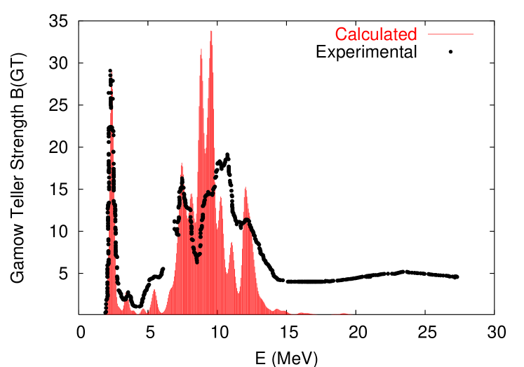
Figure 29: Gamow Teller strength in ⁴⁸Ca$(p,n)^{48}$Sc from Anderson et al. (1990)—after elimination of the Fermi peak at around 6 MeV—compared with the calculated peaks (KB3 interaction) after 700 Lanczos iterations Caurier et al. (1995b). The peaks have been smoothed by gaussians having the instrumental width of the first measured level.

The KB3 effective interaction is doing a very good job, but it is certainly not decoupling 8590 $pf$ states from the rest of the space. If the fact is not explicitly recognized we end up with the often raised Hjorth-Jensen et al. (1995) “intruder problem”: Decoupling cannot be enforced perturbatively when intruders are energetically close to model states. Figure 29 indicates that although few eigenstates are well decoupled, it is possible to make sense of many others if one interprets them as doorways. The satisfactory description of the lowest states indicates that the model space makes sense. It means that it ensures good decoupling at the $S_{2}$ level, or simply in second order perturbation theory, which guarantee a state-independent interaction.

Energetically we are in good shape, and we concentrate on the renormalization of the GT operator: the calculated strength has been quenched by a factor $\approx(0.74)^{2}$. Why? Why this factor ensures the right detailed strength for about 30 states below 8 MeV?

V.3.2 Quenching

To understand the quenching problem it is best to start by the (tentative) solution. The dressed states in Eq. (4) are normalized to unity in the model space. This trick is essential in the formulation of linked cluster or $\exp{S}$ theories (hence Eq. (63)). It makes possible the calculation of the energy—and some transitions, such as the $E2$—without knowledge of the norm of the exact wavefunction. In general though, we need an expectation value between exact, normalized states: $\langle\hat{f}\parallel{\cal T}\parallel\hat{i}\rangle^{2}$. If we write

$$|\hat{i}\rangle=\alpha|0\hbar\omega\rangle+\sum_{n\neq 0}\beta_{n}|n\hbar\omega\rangle,$$ (84)

and a similar expression in $\alpha^{\prime},\,\beta^{\prime}$ for $\langle\hat{f}|$, we find

$$\langle\hat{f}\parallel{\cal T}\parallel\hat{i}\rangle^{2}=\left(\alpha\alpha^{\prime}\,T_{0}+\sum_{n\neq 0}\beta_{n}\beta^{\prime}_{n}\,T_{n}\right)^{2},$$ (85)

since the GT operator does not couple states with different number of $\hbar\omega\,$ excitations. If we make two assumptions: (a) neglect the $n\neq 0$ contributions; (b) $\alpha\approx\alpha^{\prime}$; it follows that if the projection of the physical wavefunction in the 0$\hbar\omega\,$ space is $Q\approx\alpha^{2}$, its contribution to the transition will be quenched by $Q^{2}$.

Exactly the same arguments apply to transfer reactions—for which ${\cal T}=a_{s}$ (or $a_{s}^{\dagger}$)—but are simpler because $T_{n\neq 0}=0$. The transition strength is given by the spectroscopic factor, which can be identified with $Q$ when one particle is removed and $1-Q$ when it is added. The assumption that the model amplitudes in the exact wavefunctions are approximately constant is borne out by systematic calculations of $Q$ in the $p$ shell (Chou et al., 1993, $Q=0.820(15)$), the $sd$ shell (Wildenthal et al., 1983, $Q=0.77(2)$) and the $pf$ shell (illustrated in Fig. 30, Martínez-Pinedo et al., 1996b, $Q=0.744(15)$).

Figure 30: Comparison of the experimental and theoretical values of the quantity $T(GT)$ in the $pf$ shell Martínez-Pinedo et al. (1996b). The $x$ and $y$ coordinates correspond to theoretical and experimental values respectively. The dashed line shows the “best-fit” for $Q=0.744$. The solid line shows the result obtained in the $sd$-shell nuclei Wildenthal et al. (1983)

These numbers square well with the existing information on spectroscopic factors from $(d,p)$ (Vold et al., 1978, $Q\approx 0.7$) and $(e,e^{\prime}p)$ (Cavedon et al., 1982, $Q=0.7$) data (see also Pandharipande et al., 1997). This consistency is significant in that it backs assumption (a) above, which is trivially satisfied for spectroscopic factors. It opens the perspective of accepting the GT data as a measure of a very fundamental quantity that does not depend on particular processes. The proposed “solution” to the quenching problem amounts to reading data.

Figure 31: Effective spin g-factor of the M1 operator deduced from the comparison of shell model calculations and data for the total B(M1) strengths in the stable even mass N=28 isotones (from von Neumann-Cosel et al. (1998))

Experimentally, the challenge is to locate all the strength, constrained by the Ikeda sum rule that relates the direct and inverse processes. The careful analysis of Anderson et al. (1985) suggests, but does not prove, that the experimental tail in Fig. 29 contains enough strength to satisfy approximately the sum rule. A similar result is obtained for ⁵⁴Fe$(p,n)$ Anderson et al. (1990). More recent experiments by the Tokyo group establish that the strength located at accessible energies exhausts 90(5)% of the sum rule in the ⁹⁰Zr$(n,p)$ and 84(5)% in ²⁷Al$(p,n)$ (Wakasa et al., 1997, 1998).

The theoretical problem is to calculate $Q$. It has been compounded by a sociological one: the full GT operator is $(g_{A}/g_{V})\sigma\tau$, where $g_{A}/g_{V}\approx-1.27$ is the ratio of weak axial and vector coupling constants. The hotly debated question was whether $Q$ was due to non nucleonic renormalization of $g_{A}$ or nuclear renormalization of $\sigma\tau$ Osterfeld (1992); Arima (2001). We have sketched above the nuclear case, along the lines proposed by Caurier, Poves, and Zuker (1995b), but under a new guise that makes it easier to understand. The calculations of Bertsch and Hamamoto (1982), Drożdż et al. (1986) and Dang et al. (1997) manage to place significant amounts of strength beyond the resonance region, but they are based on 2p-2h doorways which fall somewhat short of giving a satisfactory view of the strength functions. No-core calculations are under way, that should be capable of clarifying the issue.

The purely nuclear origin of quenching is borne out by $(p,p^{\prime})$, $(\gamma,\gamma^{\prime})$ and $(e,e^{\prime})$ experiments that determine the spin and convection currents in M1 transitions, in which $g_{A}/g_{V}$ play no role (see Richter, 1995, for a complete review). An analysis of the data available for the $N=28$ isotones in terms of full $pf$-shell calculations concluded that agreement with experiment was achieved by quenching the $\sigma\tau$ operator by a factor 0.75(2), fully consistent with the value that explains the Gamow-Teller data von Neumann-Cosel et al. (1998) (see Fig. 31). These results rule out the hypothesis of a renormalization of the axial-vector constant $g_{A}$: it is the $\sigma\tau$ operator that is quenched.

VI Spherical shell model description of nuclear rotations

Theoretical studies in the $pf$ shell came in layers. The first, by McCullen, Bayman, and Zamick (1964), restricted to the $f_{7/2}$ space, was a success, but had some drawbacks: the spectra were not always symmetric by interchange of particles and holes, and the quadrupole moments had systematically the wrong sign. The first diagonalizations in the full shell [(Pasquini, 1976), (Pasquini and Zuker, 1978)] solved these problems to a large extent, but the very severe truncations necessary at the time made it impossible to treat on the same footing the pairing and quadrupole forces. The situation improved very much by dressing perturbatively the pure two-body $f_{7/2}$ part of the Hamiltonian $H_{2}$, with a three body term $H_{R1}$, mostly due to the quadrupole force Poves and Zuker (1981b). The paper ended with the phrase:

“It may well happen, that in some cases, not in the $pf$ shell but elsewhere, $H_{R1}$ will overwhelm $H_{2}$. Then, and we are only speculating, we shall speak, perhaps, of the rotational coupling scheme.”

Indeed, some nuclei were indicating a willingness to become rotational but could not quite make it, simply because the perturbative treatment was not enough for them. The authors missed prophecy by one extra conditional: “not in the $pf$ shell should have been “not necessarily…”

At the time it was thought impossible to describe rotational motion in a spherical shell-model context. The glorious exception, discovered by Elliott (1958a, b), was (apparently) associated to strict SU(3) symmetry, approximately realized only near ²⁰Ne and ²⁴Mg.

VI.1 Rotors in the $pf$ shell

Figure 32: ⁴⁸Cr level scheme; experiment $vs.$ theory

Table 8: ⁴⁸Cr; quadrupole properties of the yrast band

J	B(E2)exp	B(E2)th	Q0(t)	Q0(s)	Q0(t)[f7/2,p3/2]
2	321(41)	228	107	103	104
4	330(100)	312	105	108	104
6	300(80)	311	100	99	103
8	220(60)	285	93	93	102
10	185(40)	201	77	52	98
12	170(25)	146	65	12	80
14	100(16)	115	55	13	50
16	37(6)	60	40	15	40

The fourth layer was started when the ANTOINE code (Section III.4) came into operation: ⁴⁸Cr was definitely a well deformed rotor Caurier et al. (1994), as can be surmised by comparing with the experimental spectrum from  Lenzi et al. (1996) in Fig. 32  (see also Cameron et al., 1993) and the transition properties in Table 8 from  Brandolini et al. (1998) where we have used

$$Q_{0}(s)=\frac{(J+1)\,(2J+3)}{3K^{2}-J(J+1)}\,Q_{spec}(J),\quad K\neq 1$$ (86)

$$B(E2,J\;\rightarrow\;J-2)=$$

$$\frac{5}{16\pi}\,e^{2}|\langle JK20|J-2,K\rangle|^{2}\,Q_{0}(t)^{2}\quad K\neq 1/2,\,1;$$ (87)

to establish the connection with the intrinsic frame descriptions: A good rotor must have a nearly constant $Q_{0}$, which is the case up to $J=10$, then ⁴⁸Cr backbends. This is perhaps the most striking result to come out of our $pf$ calculations, because such a behaviour had been thought to occur only in much heavier nuclei.

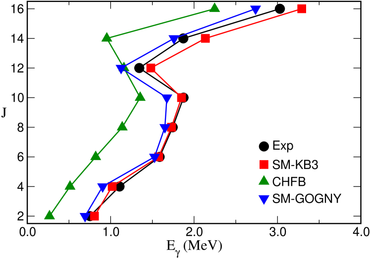
Figure 33: The yrast band of ⁴⁸Cr; experiment vs. the shell model calculations with KB3 and the Gogny force and the CHFB results also with the Gogny force.

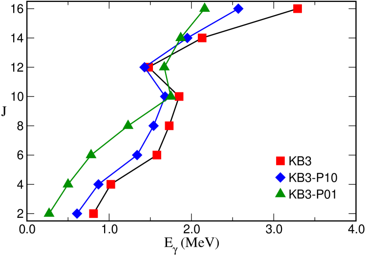
Figure 34: Gamma-ray energies along the yrast band of ⁴⁸Cr (in MeV), full interaction (KB3), isoscalar pairing retired (KB3–P01) and isovector pairing retired (KB3–P01).

Fig. 33 compares the experimental patterns with those obtained with KB3, and with the Gogny force. The latter, when diagonalized gives surprisingly good results. When treated in the cranked Hartree Fock Bogoliubov (CHFB) approximation, the results are not so good. The discrepancy is more apparent than real: The predictions for the observables are very much the same in both cases (see Caurier et al., 1995a, for the details). The reason is given in Fig 34, where exact KB3 diagonalizations are done, subtracting either of the two pairing contributions, $JT=01$ and 10 Poves and Martínez-Pinedo (1998). It is apparent that the $JT=01$-subtracted pattern is quite close to the CHFB one in Fig. 33, especially in the rotational regime before the backbend. The $JT=10$ subtraction goes in the same direction. The interpretation is transparent: CHFB does not “see” proton-neutron pairing at all, and it is not very efficient in the low pairing regime. As it does everything else very well, the inevitable conclusion is that pairing can be treated in first order perturbation theory, i.e., the energies are very sensitive to it, but not the wavefunctions. Floods of ink have gone into “neutron-proton” pairing, which is a problem for mean field theories but neither for the Gogny force nor for the shell model. Furthermore, the results show that ordinary pairing is also a mean field problem when nuclei are not superfluids.

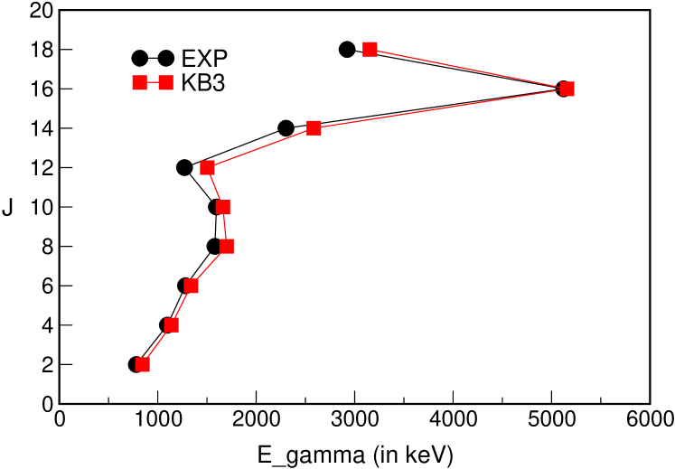
Figure 35: The yrast band of ⁵⁰Cr; experiment vs. the shell model calculations with the KB3 interaction

⁴⁸Cr has become a standard benchmark for models (Cranked Hartree Fock Bogoliuvov Caurier et al. (1995a), Cranked Nilsson Strutinsky Juodagalvis and Åberg (1998), Projected Shell Model Hara et al. (1999), Cluster Model Descouvemont (2002), etc.) Nuclei in the vicinity also have strong rotational features. The mirror pairs ⁴⁷V-⁴⁷Cr and ⁴⁹Cr-⁴⁹Mn closely follow the semiclassical picture of a particle or hole hole strongly coupled to a rotor  (Martínez-Pinedo et al., 1997) in full agreement with the experiments Cameron et al. (1991, 1994); O’Leary et al. (1997); Bentley et al. (1998); Tonev et al. (2002). ⁵⁰Cr was predicted to have a second backbending by Martínez-Pinedo et al. (1996a), confirmed experimentally Lenzi et al. (1997) (see figure 35). When more particles or holes are added, the collective behaviour fades, though even for ⁵²Fe, a rotor like band appears at low spin with an yrast trap at J=12⁺, both are accounted for by the shell model calculations Poves and Zuker (1981b)(sic), Ur et al. (1998). For spectroscopic comparisons with the odd-odd nuclei, see Lenzi et al. (1999); Brandolini et al. (2001) for ⁴⁶V and Svensson et al. (1998) for ⁵⁰Mn. Recently, a highly deformed excited band has been discovered in ⁵⁶Ni Rudolph et al. (1999). It is dominated by the configuration (1f_7/2)¹² (2p_3/2, 1f_5/2, 2p_1/2)⁴. The calculations reproduce the band, that starts at about 5 MeV excitation energy and has a deformation close to $\beta$=0.4.

VI.2 Quasi-SU(3).

To account for the appearance of backbending rotors, a theoretical framework was developed by Zuker et al. (1995), and made more precise by Martínez-Pinedo et al. (1997). Here we give a compact overview of the scheme that will be shown to apply even to the classic examples of rotors in the rare-earth region.

Let us start by considering the quadrupole force alone, taken to act in the $p$-th oscillator shell. It will tend to maximize the quadrupole moment, which means filling the lowest orbits obtained by diagonalizing the operator $Q_{0}=2q_{20}=2z^{2}-x^{2}-y^{2}$. Using the cartesian representation, $2q_{20}=2n_{z}-n_{x}-n_{y}$, we find eigenvalues $2p$, $2p-3$,…, etc., as shown in the left panel of Fig. 36, where spin has been included. By filling the orbits orderly we obtain the intrinsic states for the lowest SU(3) representations Elliott (1958a, b): $(\lambda,0)$ if all states are occupied up to a given level and $(\lambda,\mu)$ otherwise. For instance: putting two neutrons and two protons in the $K=1/2$ level leads to the ($4p$,0) representation. For four neutrons and four protons, the filling is not complete and we have the (triaxial) ($8(p-1)$,4) representation for which we expect a low lying $\gamma$ band.

Figure 36: Nilsson orbits for SU(3) $(k=-2p)$ and quasi-SU(3) ($k=-2p+1/2)$).

In $jj$ coupling the angular part of the quadrupole operator $q^{20}=r^{2}C^{20}$ has matrix elements

$$\langle j\,m|C^{2}|j+2\,m\rangle\approx\frac{3[(j+3/2)^{2}-m^{2}]}{2(2j+3)^{2}},$$ (88)

$$\quad\langle j\,m|C^{2}|j+1\,m\rangle=-\frac{3m[(j+1)^{2}-m^{2}]^{1/2}}{2j(2j+2)(2j+4)}$$ (89)

The $\Delta j=2$ numbers in Eq. (88) are—within the approximation made—identical to those in $LS$ scheme, obtained by replacing $j$ by $l$. The $\Delta j=1$ matrix elements in Eq. (88) are small, both for large and small $m$, corresponding to the lowest oblate and prolate deformed orbits respectively. If the spherical $j$-orbits are degenerate, the $\Delta j=1$ couplings, though small, will mix strongly the two $\Delta j=2$ sequences (e.g., $(f_{7/2}p_{3/2})$ and $(f_{5/2}p_{1/2})$). The spin-orbit splittings will break the degeneracies and favour the decoupling of the two sequences. Hence the idea (Zuker et al., 1995) of neglecting the $\Delta j=1$ matrix elements and exploit the correspondence

$$l\longrightarrow j=l+1/2\quad m\longrightarrow m+1/2\times{\rm sign}(m).$$

which is one-to-one except for $m=0$. The resulting “quasi SU(3)” quadrupole operator respects SU(3) relationships, except for $m=0$, where the correspondence breaks down. The resulting spectrum for quasi-$2q_{20}$ is shown in the right panel of Fig 36. The result is not exact for the $K=1/2$ orbits but a very good approximation.

To check the validity of the decoupling, a Hartree calculation was done for $H=\varepsilon H_{sp}+H_{q}$, where $H_{sp}$ is the observed single particle spectrum in ⁴¹Ca (essentially equidistant orbits with 2MeV spacings) and $H_{q}$ is the quadrupole force in Eq. (33) with a properly renormalized coupling. The result is exactly a Nilsson (1955) calculation Martínez-Pinedo et al. (1997),

$$H_{Nilsson}=\hbar\omega\left(\varepsilon H_{sp}-\frac{\delta}{3}\,2q_{20}\right),$$ (90)

where

$$\frac{\delta}{3}=\frac{1}{4}\frac{\langle 2q_{20}\rangle}{\langle r^{2}\rangle}=\frac{\langle 2q_{20}\rangle}{(p+3/2)^{4}}.$$ (91)

In the right panel of Fig. 37 the results are given in the usual form.

Figure 37: Nilsson diagrams in the $pf$ shell. Energy vs. single particle splitting $\varepsilon$ (left panel), energy vs. deformation $\delta$ (right panel).

In the left panel we have turned the representation around: since we are interested in rotors, we start from perfect ones (SU(3)) and let $\varepsilon$ increase. At a value of $\approx 0.8$ the four lowest orbits are in the same sequence as the right side of fig. 36 (Remember here that the real situation corresponds to $\varepsilon\approx 1.0$). The agreement even extends to the next group, although now there is an intruder (1/2[310] orbit). The suggestion is confirmed by an analysis of the wavefunctions: For the lowest two orbits, the overlaps between the pure quasi-SU(3) wavefunctions calculated in the restricted $\Delta j=2$ space ($fp$ from now on) and the ones in the full $pf$ shell exceeds 0.95 throughout the interval $0.5<\varepsilon<1$. More interesting still: the contributions to the quadrupole moments from these two orbits vary very little, and remain close to the values obtained at $\varepsilon=0$ i.e., from fig. 36).

Figure 38: Yrast transition energies $E_{\gamma}=E(J+2)-E(J)$ for different configurations, KLS interaction.

Figure 39: Backbending patterns in $(gds)^{8}$ $T=0$, with the KLS interaction and with a random interaction plus a constant $W_{rstu}^{JT}=-a$.

We have learned that –for the rotational features– calculations in the restricted $(fp)^{n}$ spaces account remarkably well for the results in the full major shell $(pf)^{n}$ (see last column of Table 8). Let us move now to larger spaces. In Fig. 38 we have yrast transition energies for different configurations of 8 particles in $\Delta j=2$ spaces. The force is KLS, $\hbar\omega=9$ MeV, the single particle splittings uniform at $\varepsilon=1$ MeV, and $gds$, say, is the lower sequence in the $sdg$, $p=4$, shell. Rotational behavior is fair to excellent at low $J$. As expected from the normalization property of the realistic quadrupole force [Eq. (35)] the moments of inertia in the rotational region go as $(p+3/2)^{2}\,(p^{\prime}+3/2)^{2}$, i.e. if we multiply all the $E_{\gamma}$ values by this factor the lines become parallel. The intrinsic quadrupole moment $Q_{0}$ [Eq. (86)] remains constant to within 5% up to a critical $J$ value at which the bands backbend.

Why and how do the bands backbend? We have no simple answer, but Fig. 39 from (Velázquez and Zuker, 2002) shows the behavior of the $(gds)^{8}$ space under the influence of a symmetric random interaction, gradually made more attractive by an amount $a$. There is no need to stress the similarity with Fig. 38. The appearance of backbending rotors seems to be a general result of the competition between deformation and alignment, characteristic of nuclear processes.

The group theoretical aspects of quasi-SU3 have been recently discussed and applied to the description of the $sd$-shell nuclei by Vargas, Hirsch, and Draayer (2001); Vargas, Hirsch, and Draayer (2002a).

VI.3 Heavier nuclei: quasi+pseudo SU(3)

We have seen that quasi-SU(3) is a variant of SU(3) that obtains for moderate spin-orbit splittings. For other forms of single particle spacings, the pseudo-SU(3) scheme (Arima et al. (1969); Hecht and Adler (1969); Raju et al. (1973), see also Vargas et al. (2002b) for more recent applications) will be favored (in which case we have to use the left panel of Fig. 36, with pseudo-$p=p-1$). Other variants of SU(3) may be possible and are well worth exploring. In cases of truly large deformation SU(3) itself may be valid in some blocks.

To see how this works, consider Fig. 40 giving a schematic view of the single particle energies in the space of two contiguous major shells—in protons ($\pi$) and neutrons ($\nu$)—adequate for a SM description of the rare earth region.

Figure 40: Schematic single particle spectrum above ¹³²Sn. $r_{p}$ is the set of orbits in shell $p$ excluding the largest. For the upper shells the label $l$ is used for $j=l+1/2$

We want to estimate the quadrupole moments for nuclei at the onset of deformation. We shall assume quasi-SU(3) operates in the upper shells, and pseudo-SU(3) in the lower ones. The number of particles in each shell for which the energy will be lowest will depend on a balance of monopole and quadrupole effects, but Nilsson diagrams suggest that when nuclei acquire stable deformation, two orbits $K$=1/2 and 3/2—originating in the upper shells of Fig. 36—become occupied, i.e., the upper blocks are precisely the 8-particle configurations we have studied at length. Their contribution to the electric quadrupole moment is then

$$Q_{0}=8[e_{\pi}(p_{\pi}-1)+e_{\nu}(p_{\nu}-1)],$$ (92)

with $p_{\pi}=5$, $p_{\nu}=6$; $e_{\pi}$ and $e_{\nu}$ are the effective charges.

Consider even-even nuclei with Z=60-66 and N=92-98, corresponding to 6 to 10 protons with pseudo-$p=3$, and 6 to 10 neutrons with pseudo-$p=4$ in the lower shells. From the left part of Fig. 36 we obtain easily their contribution to $Q_{0}$, which added to that of Eq. (92) yields a total

$$Q_{0}=56e_{\pi}+(76+4n)e_{\nu},$$ (93)

for ¹⁵²⁺²ⁿNd, ¹⁵⁴⁺²ⁿSm, ¹⁵⁶⁺²ⁿGd and ¹⁵⁸⁺²ⁿDy respectively. At fixed $n$, the value is constant in the four cases because the orbits of the triplet K=1/2, 3/2, 5/2 in Fig. 36 have zero contribution for $p$=3. $Q_{0}$ (given in dimensionless oscillator coordinates, i.e., $r\rightarrow r/b$ with $b^{2}\approx 1.01{\rm A}^{-1/3}fm^{2}$), is related to the $E2$ transition probability from the ground state by $B(E2)\uparrow=10^{-5}{\rm A}^{2/3}Q_{0}^{2}$. The results, using effective charges of $e_{\pi}=1.4$, $e_{\nu}=0.6$ calculated in (Dufour and Zuker, 1996) are compared in table 9 with the available experimental values . The agreement is quite remarkable and no free parameters are involved. Note in particular the quality of the prediction of constancy (or rather $A^{2/3}$ dependence) at fixed $n$, which does not depend on the choice of effective charges. The discrepancy in ¹⁵²Nd is likely to be of experimental origin, since systematics indicate, with no exception, much larger rates for a $2^{+}$ state at such low energy (72.6 keV).

Table 9: $B(E2)\uparrow$ in $e^{2}b^{2}$ compared with experiment Raman et al. (1989)

N	Nd	Sm	Gd	Dy
92	4.47	4.51	4.55	4.58
	2.6(7)	4.36(5)	4.64(5)	4.66(5)
94	4.68	4.72	4.76	4.80
			5.02(5)	5.06(4)
96	4.90	4.95	4.99	5.03
			5.25(6)	5.28(15)
98	5.13	5.18	5.22	5.26
				5.60(5)

It is seen that by careful analysis of exact results one may come to very simple computational strategies. In the last example on B(E2) rates, the simplicity is such that the computation reduces to a couple of sums.

VI.4 The ³⁶Ar and ⁴⁰Ca super-deformed bands

The arguments sketched above apply to the region around ¹⁶O, where a famous 4-particles 4-holes (4p-4h) band starting at 6.05 MeV was identified by Carter et al. (1964), followed by the 8p-8h band starting at 16.75 MeV Chevallier et al. (1967). Shell model calculations in a very small space, $p_{1/2}d_{5/2}s_{1/2}$, could account for the spectroscopy in ¹⁶O, including the 4p-4h band (Zuker et al., 1968, ZBM), but the 8p-8h one needs at least three major shells and was tackled by an $\alpha$-cluster model Abgrall et al. (1967b, a). It is probably the first superdeformed band detected and explained.

In ⁴⁰Ca, the first excited $0^{+}$ state is the 4p-4h band-head. It is only recently that another low-lying highly deformed band has been found Ideguchi et al. (2001), following the discovery of a similar structure in ³⁶Ar Svensson et al. (2000).

By applying the quasi+pseudo-SU(3) recipes of Section VI.3 we find that the maximum deformations attainable are of 8p-8h character in ⁴⁰Ca and 4p-4h in ³⁶Ar with $Q_{0}=180$ efm² and $Q_{0}=136$ efm² respectively.

The natural generalization of the ZBM space consists in the $d_{3/2}s_{1/2}fp$ orbits (remember: $fp\equiv f_{7/2}p_{3/2}$), which is relatively free of center of mass spuriousness. And indeed, it describes well the rotational regime of the observed bands. However, to track them beyond backbend, it is convenient to increase the space to $d_{3/2}s_{1/2}pf$. The adopted interaction, sdfp.sm is the one originally constructed by Retamosa et al. (1997), and used in Caurier et al. (1998) (USD, KB3 for intra shell and KLS for cross shell matrix elements), with minor monopole adjustments dictated by new data on the single particle structure of ³⁵Si Nummela et al. (2001a).

The calculations are conducted in spaces of fixed number of particles and holes. In figure 41 the calculated energy levels in ³⁶Ar are compared to the data. The agreement is excellent, except at $J=12$ where the data show a clear backbending while the calculation produces a much smoother upbending pattern.

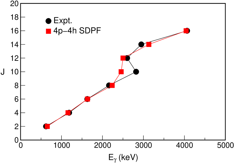
Figure 41: The superdeformed band of ³⁶Ar, experiment vs. SM

In table 10 the calculated spectroscopic quadrupole moments ($Q_{s}$) and the B(E2)’s are used to compute the intrinsic $Q$ as in Eqs. (86,87), using standard effective charges $\delta q_{\pi}$=$\delta q_{\nu}$=0.5. As expected both Q₀(s) and Q₀(t) are nearly equal and constant—and close to the quasi+pseudo SU(3) estimate—up to the backbend. The calculated B(E2)’s agree well with the experimental ones Svensson et al. (2001). The value of $Q_{0}$ corresponds to a deformation $\beta\approx 0.5$.

Table 10: Quadrupole properties of the 4p-4h configuration’s yrast-band in ³⁶Ar (in e²fm⁴ and efm²)

	B(E2)(J$\rightarrow$J-2)
J	EXP	TH	Qspec	Q0(s)	Q0(t)
2		315	-36.0	126	126
4	372(59)	435	-45.9	126	124
6	454(67)	453	-50.7	127	120
8	440(70)	429	-52.8	125	114
10	316(72)	366	-52.7	121	104
12	275(72)	315	-53.0	119	96
14	232(53)	235	-54.3	120	82
16	$>$84	131	-56.0	122	61

Now we examine the 8p-8h band in ⁴⁰Ca Ideguchi et al. (2001). The valence space adopted for ³⁶Ar is truncated by limiting the maximum number of particles in the 1f_5/2 and 2p_1/2 orbits to two.

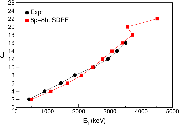
Figure 42: The superdeformed band in ⁴⁰Ca; exp. vs. 8p-8h calculation

The experimental Ideguchi et al. (2001) and calculated yrast gamma-ray energies are compared in fig. 42. The patterns agree reasonably well but the change of slope at $J=10$ —where the backbend in ⁴⁸Cr starts (Fig. 33)—is missed by the calculation, which only backbends at $J=20$, the band termination for the configuration $f_{7/2}^{8}(d_{3/2}s_{1/2})^{-8}$. The extra collectivity induced by the presence of $sd$ particles in pseudo-SU(3) orbitals is responsible or the delay in the alignment, but apparently too strong to allow for the change in slope at $J=10$.

Table 11: Quadrupole properties of the 8p-8h configuration’s yrast-band in ⁴⁰Ca (in e²fm⁴ and efm²), calculated in the $sdpf$ valence space

J	B(E2)(J $\rightarrow$ J-2)	Qspec	Q0(t)	Q0(s)
2	589	-49.3	172	172
4	819	-62.4	170	172
6	869	-68.2	167	171
8	860	-70.9	162	168
10	823	-71.6	157	164
12	760	-71.3	160	160
14	677	-71.1	149	157
16	572	-72.2	128	158
18	432	-75.0	111	162
20	72	-85.1
22	8	-79.1
24	7	-81.5

The experimental $Q_{0}$(t)=180${}^{+39}_{-29}$ obtained from the fractional Doppler shifts corresponds to a deformation $\beta\approx 0.6$ Ideguchi et al. (2001). It is extracted from an overall fit that assumes constancy for all measured values, and corresponds exactly to the quasi+pseudo SU(3) estimate. It also squares well with the calculated 172 efm² in Table 11 where the steady decrease in collectivity remains consistent with experiment within the quoted uncertainties. A reanalysis of the experimental lifetimes in the superdeformed band of ⁴⁰Ca Chiara et al. (2003) suggest that for low spins the deformation would be smaller due to the mixing with less deformed states of lower np-nh rank.

This calculation demonstrates that a detailed description of very deformed bands is within reach of the shell model. The next step consists in remembering that states at fixed number of particles are doorways that will fragment in an exact calculation that remains to be done.

The band in ³⁶Ar has been also described by the projected shell model in Long and Sun (2001). Beyond mean field methods using the Skyrme interaction have been recently applied to both the ³⁶Ar and ⁴⁰Ca superdeformed bands by Bender, Flocard, and Heenen (2003a).

VI.5 Rotational bands of unnatural parity

The occurrence of low-lying bands of opposite parity to the ground state band is very frequent in $pf$ shell nuclei. Their simplest characterization is as particle-hole bands with the hole in the 1d_3/2 orbit. In a nucleus whose ground state is described by the configurations $(pf)^{n}$ the opposite parity intruders will be (1d_3/2)^-1 $(pf)^{n+1}$. The promotion of a particle from the $sd$ to the $pf$ shell costs an energy equivalent to the local value of the gap, that in this region is about 7 MeV. On the other side, the presence of one extra particle in the $pf$-shell may produce an important increase of the correlation energy, that can compensate the energy lost by the particle hole jump. For instance, the very low-lying positive parity band of ⁴⁷V, can be interpreted as (1d_3/2)^-1 (a proton hole) coupled to $(pf^{8})$ T=0. Indeed, the correlation energy of this pseudo-⁴⁸Cr is larger than the correlation energy of the ground state of ⁴⁷V and even larger than the correlation energy of the real ⁴⁸Cr, explaining why the band starts at only 260 keV of excitation energy Poves and Sánchez Solano (1998). The most extreme case is ⁴⁵Sc, where the intruder band based in the configuration (1d_3/2)^-1 coupled to ⁴⁶Ti, barely miss (just by 12 keV) to become the ground state. Many bands of this type have been experimentally studied in recent years, mainly at the Gasp and Euroball detectors Brandolini et al. (1999), and explained by shell model calculations.

Figure 43: The ground state (K=4⁺) and the side band (K=1⁺) of ⁴⁸V, experiment $vs.$ theory.

We present now some recent results in ⁴⁸V Brandolini et al. (2002a). The positive parity levels of this odd-odd nucleus are very well reproduced by the shell model calculation using the interactions KB3 (or KB3G) as can be seen in Fig. 43, another example of good quality “pure spectroscopy”. The levels are grouped in two bands, one connected to the 4⁺ ground state, that would correspond to K=4⁺ in a Nilsson context (the aligned coupling of the last unpaired proton K=3/2^- and the last neutron K=5/2^-) and a second one linked to the 1⁺ member of the ground state multiplet that results of the anti-aligned coupling.

Figure 44: The negative parity K=1^- and K=4^- bands of ⁴⁸V, experiment $vs.$ theory.

The negative parity states can be interpreted as the result of the coupling of a hole in the 1d_3/2 orbit to ⁴⁹Cr. As we have mentioned earlier, the ground state band of ⁴⁹Cr can be understood in a particle plus rotor picture, and assigned K=5/2^-. Now we have to couple the 1d_3/2 hole to our basic rotor ⁴⁸Cr. Therefore the structure of the negative parity states of ⁴⁸V is one particle and one hole coupled to the rotor core of ⁴⁸Cr. Hence we expect that the lowest lying bands would have K=1^- and K=4^- (aligned and anti-aligned coupling of the quasiparticle and the quasihole). These two bands have been found experimentally at about 500 keV of excitation energy. Their structure is in very good agreement with the SM predictions (see Fig. 44) except for a small shift of the K=4^- and K=8^- bandheads relative to the K=1^- state.

Figure 45: Theoretical and experimental B(M1) and B(E2) transition probabilities in the ground state band of ⁴⁸V

A more stringent test of the theoretical predictions is provided by the electromagnetic properties. In this particular nucleus the experimental information is very rich and a detailed comparison can be made for both the positive and negative bands and for E2 and M1 transitions. The results for the ground state band are collected in Fig. 45. Notice that the calculation reproduces even the tiniest details of the experimental results, as, for instance the odd-even staggering of the B(M1)’s. The B(E2)’s correspond to a deformation $\beta$=0.2 that is clearly smaller than that of ⁴⁸Cr.

Figure 46: Theoretical and experimental B(M1) and B(E2) transition probabilities in the negative parity bands of ⁴⁸V

The transition probabilities in the negative parity bands are presented in Fig. 46. Now the experimental results have larger uncertainties. Despite that, the agreement in absolute values and trends is very good for the lowest band (K=1^-). The quantitative agreement is worse for the other two bands, nevertheless, the main features of the data are well reproduced. The deformation of the K=1^- band extracted from the B(E2) properties turns out to be larger than the deformation of the ground state band and close to that of ⁴⁸Cr.

VII Description of very neutron rich nuclei

The study of nuclei lying far from the valley of stability is one of the most active fields in today’s experimental nuclear physics. What it specific about these nuclei, from a shell model point of view? As everywhere else: the model space and the monopole behavior of the interaction. They go together because the effective single particle energies (ESPE, see Section V) depend on occupancies, which in turn depend on the model space.

In broad terms, the specificity of light and medium neutron rich nuclei is that the EI closures (corresponding to the filling of the $p+1/2$ orbit of each oscillator shell) take over as boundaries of the model spaces. As discussed in Section II.2.2, the oscillator closures (HO) may be quite solid for double magic nuclei, but they become vulnerable in the semi-magic cases.

For instance the $d_{3/2}$-$f_{7/2}$ neutron gap in ⁴⁰Ca of $\approx 7$ MeV goes down to $\approx 2.5$ MeV around ²⁸O. Since the $d_{5/2}$ orbit is well below its $sd$ partners, now quite close to $f_{7/2}$, the natural model space is no longer the $sd$ shell, but the EI space bounded by the $N=14$ and 28 closures, supplemented by the $p_{3/2}$ subshell whenever the $p_{3/2}$-$f_{7/2}$ gap becomes small: from $\approx 6$ MeV in ⁵⁶Ni, it drops to $\approx 4.5$ MeV in ⁴⁸Ca, then $\approx 2$ MeV in ⁴⁰Ca, and finally $\approx 0$ MeV in ²⁸Si. As explained at the end of Section II.2.2 this monopole drift provides direct evidence for the need of three-body mechanisms.

For the $p$ shell, the situation is similar: The imposing 11.5 MeV $p_{1/2}$-$d_{5/2}$ gap in ¹⁶O is down to some 3 MeV in ¹²C. The monopole drift of the $s_{1/2}$-$d_{5/2}$ gap brings it from about 8 MeV in ²⁸Si to nearly -1 MeV in ¹²C. According to Otsuka et al. (2001a) the drift may well continue: in ⁸He, the $s_{1/2}$-$p_{1/2}$ bare gap is estimated at 0.8 MeV.

All the numbers above (except the last) are experimental. The bare monopole values are smaller because correlations increase substantially the value of the gaps, but they do not change qualitatively the strong monopole drifts. Their main consequence is that “normal” states, i.e., those described by 0$\hbar\omega\,$ $p$ or $sd$ calculations often “coexist” with “intruders” that involve promotion to the next oscillator shell. Let us examine how this happens.

VII.1 N=8; ¹¹Li: halos

The 1/2⁺ ground state in ¹¹Be provided one of the first examples of intrusion. The expected 0$\hbar\omega$ normal state lies 300 keV higher. The explanation of this behavior has varied with time Talmi and Unna (1960); Sagawa et al. (1993); Suzuki and Otsuka (1994); Aumann et al. (2001), see also (Brown, 2001) for a recent review and Suzuki et al. (2003) for a new multi-$\hbar\omega\,$calculation, but the idea has remained unchanged. The normal state corresponds to a hole on the $N=8$ closure. The monopole loss of promoting a particle to the $sd$ shell is compensated by a pairing gain for the $p_{1/2}^{-2}$ holes. A quadrupole gain due to the interaction of the $sd$ neutron with the $p^{2}$ protons is plausible, but becomes questionable when we note that the same phenomenon occurs in ⁹He which has no $p^{2}$ particles, suggesting the need for a further reduction of the monopole loss Otsuka et al. (2001a).

The interest in ¹¹Be—as a “halo” nucleus—was revived by the discovery of the remarkable properties of ¹¹Li, which sits at the drip line ($\approx$ 200 keV two-neutron separation energy) and has a very large spatial extension, due to a neutron halo Tanihata et al. (1985); Hansen and Jonson (1987).

The shell model has no particular problem with halo nuclei, whose large size is readily attributed to the large size of the $s_{1/2}$ orbit. As shown by Kahana et al. (1969a) the use of Woods Saxon wavefunctions affect the matrix elements involving this orbit, but the uncertainties involved are easily absorbed by the monopole field. As a consequence, the whole issue hinges on the $s_{1/2}$ contribution to the wavefunctions, which is sensitively detected by the $\beta$ decay to the first excited 1/2^- state in ¹¹Be. In Borge et al. (1997) it was shown that calculations producing a 50% split between the neutron closed shell and the $s_{1/2}^{2}\,p_{1/2}^{-2}$ configuration lead to the right lifetime. This result was confirmed by Simon et al. (1999). Further confirmation comes from Navin et al. (2000), with solid indications that the supposedly semi-magic ¹²Be ground state is dominated by the same $s_{1/2}^{2}\,p_{1/2}^{-2}$ configuration.

VII.2 N=20; ³²Mg, deformed intruders

In the mid 1970’s it was the $sd$ shell that attracted the most attention. Nobody seemed to remember ¹¹Be, and everybody (including the authors of this review active at the time) were enormously surprised when a classic experiment Thibault et al. (1975) established that the mass and $\beta$-decay properties of the ³¹Na ground state—expected to be semimagic at $N=20$—could not possibly be that of a normal state Wildenthal and Chung (1979). The next example of a frustrated semi-magic was ³²Mg  Detraz et al. (1979). Early mean field calculations had interpreted the discrepancies as due to deformation Campi et al. (1975) but the experimental confirmation took some time Guillemaud-Mueller et al. (1984); Klotz et al. (1993); Motobayashi et al. (1995).

Exploratory shell model calculations by Storm et al. (1983), including the 1f_7/2 orbit in the valence space, was able to improve the mass predictions, however, deformation was still absent. To obtain deformed solutions demanded the inclusion of the 2p_3/2 orbit as demonstrated by Poves and Retamosa (1987). These calculations were followed by many others Warburton et al. (1990); Heyde and Woods (1991); Fukunishi et al. (1992); Poves and Retamosa (1994); Otsuka and Fukunishi (1996); Siiskonen et al. (1999), that mapped an “island of inversion”, i.e. the region where the intruder configurations are dominant in the ground states. The detailed contour of this “island” depends strongly on the behavior of the effective single particle energies (ESPE), in turn dictated by the monopole hamiltonian. Let’s recall, that according to what we have learned in Section VI.2, the configurations $(d_{5/2}s_{1/2})^{2-4}_{p}\,(f_{7/2}p_{3/2})^{2-4}_{n}$,corresponding to $N=20,\,Z=10$-12, have a “quasi-SU(3)” quadrupole coherence close to that of SU(3) (i.e., maximal).

The ESPE in Fig. 47 represent $H_{m}$ for the sdfp.sm and Tokyo group interactions Utsuno et al. (1999). Within details they are quite close, and such as efficiently to favor deformation. Both interactions lead to an “island of inversion” for $Z$=10, 11 and 12; $N$=19, 20 and 21.

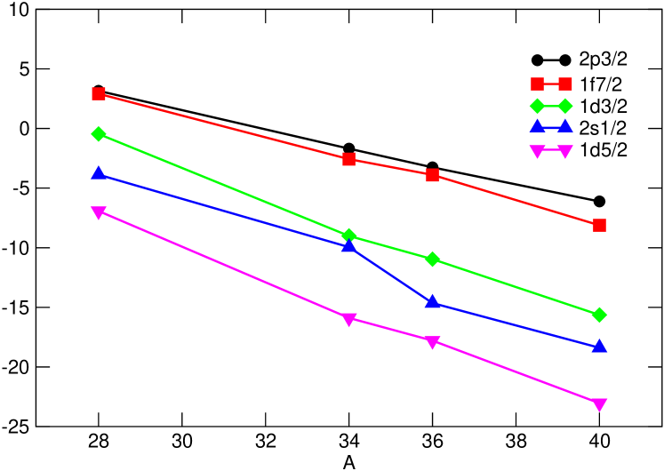
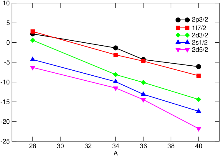
Figure 47: Effective single particle energies (in MeV) at N=20 with the $sdpf.sm$ interaction (upper panel) and the Tokyo group interaction (bottom panel)

Consider now some detailed information obtained with $sdpf.sm$ by Caurier et al. (2001c). The $S_{2N}$ values of Fig. 48 locate the neutron drip line, consistent with what is known for oxygen and fluorine, where the last bound isotopes are ²⁴O and ³¹F Sakurai et al. (1999). Note the kink due to deformed correlations in the latter. For the other chains, the behavior is smoother and the last predicted bound isotopes are ³⁴Ne, ³⁷Na and ⁴⁰Mg.

Table 12: Properties of the even magnesium isotopes. N stands for normal and I for intruder. Energies in MeV, B(E2)’s in e²fm⁴ and Q’s in efm²

		30Mg			32Mg			34Mg
	N	I	EXP	N	I	EXP	N	I	EXP
$\Delta$E(0${}^{+}_{\textrm{I}}$)		+3.1			-1.4			+1.1
0+	0.0	0.0		0.0	0.0		0.0	0.0
2+	1.69	0.88	1.48	1.69	0.93	0.89	1.09	0.66	0.67
4+	4.01	2.27		2.93	2.33	(2.29)	2.41	1.86	2.13
6+	6.82	3.75		9.98	3.81		3.52	3.50
B(E2)
2+ $\rightarrow$ 0+	53	112	59(5)	36	98	90(16)	75	131	126(25)
4+ $\rightarrow$ 2+	35	144		17	123		88	175
6+ $\rightarrow$ 4+	23	140		2	115		76	176
Qspec(2+)	-12.4	-19.9		-11.4	-18.1		-15.4	-22.7

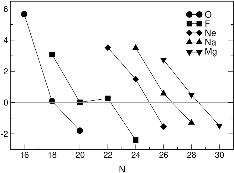
Figure 48: Two neutron separation energies (in MeV) calculated with the $sdpf.sm$ interaction.

Some results for the even Mg isotopes (N=18, N=20 and N=22) are gathered in table 12. In ³⁰Mg the normal configuration is the one that agrees with the existing experimental data Pritychenko et al. (1999). In ³²Mg the situation is the opposite as the experimental data (the 2⁺ excitation energy Guillemaud-Mueller et al. (1984) and the 0⁺ $\rightarrow$ 2⁺ B(E2) Motobayashi et al. (1995)) clearly prefer the intruder. A preliminary measure of the 4⁺ excitation energy reported by Azaiez (1999) goes in the same direction. Data and calculations suggest prolate deformation with $\beta\approx$ 0.5. In ³⁴Mg the normal configuration that contains two $pf$ neutrons, is already quite collective. It can be seen in the table that it resembles the ³²Mg ground state. The 4p-2h intruder is even more deformed ($\beta\approx$ 0.6) and a better rotor. Results from the Riken experiments of Yoneda et al. (2000) and Iwasaki et al. (2001) seem to favor the intruder option. In the QMCD calculations of Utsuno et al. (1999), the ground state band is dominantly 4p-2h; the 2⁺ comes at the right place, but the 4⁺ is too high. Clearly, ³⁴Mg is at the edge of the “island of inversion”. Another manifestation of the intruder presence in the region has been found at Isolde Nummela et al. (2001b): The decay of ³³Na indicates that the ground state of ³³Mg has J^π=3/2⁺ instead of the expected J^π=3/2^- or J^π=7/2^-. This inversion is nicely reproduced by the $sdpf.sm$ calculation.

VII.3 N=28: Vulnerability

Let us return for a while on Fig. 47. The scale does not do justice to a fundamental feature: the drift of the $p_{3/2}-f_{7/2}$ gap, which decreases as protons are removed. As explained at the end of Section II.2.2, this behavior is contrary to a very general trend in heavier nuclei, and demands a three-body mechanism to resolve the contradiction. Next we remember that the oscillator closures are quite vulnerable even at the strict monopole level. As we have seen, quadrupole coherence takes full advantage of this vulnerability. On the contrary, the EI closures are very robust. However, because of the drift of the $p_{3/2}-f_{7/2}$ gap even the $N=28$ closure becomes vulnerable. The $sdpf.sm$ interaction leads to a remarkable result summarized in Table 13: the decrease of the gap combined with the gain of correlation energy of the 2p-2h lead to a breakdown of the $N=28$ closure for ⁴⁴S and ⁴⁰Mg. The double magic ⁴²Si resists. Towards N=Z, ⁵²Cr and ⁵⁴Fe exhibit large correlation energies associated to the prolate deformed character of their 2p-2h neutron configurations ($\beta\sim$ 0.3).

When the 2p-2h bandheads of ⁴⁰Mg and ⁵²Cr are allowed to mix in the full 0$\hbar\omega$ space, using them as pivots in the LSF procedure, they keep their identity to a large extent. This can be seen in Fig. 49, where we have plotted the strength functions of the 2p-2h 0⁺ states in the full space. In ⁴⁰Mg the 2p-2h state represents the 60% of the ground state while in ⁵²Cr it is the dominant component (70%) of the first excited 0⁺. This is a very interesting illustration of the mechanism of intrusion; the intruder state is present in both nuclei, but it is only in the very neutron rich one that it becomes the ground state.

Figure 49: LSF of the 2p-2h 0⁺ bandheads of ⁴⁰Mg (upper panel) and ⁵²Cr (bottom panel) in the full 0$\hbar\omega$ space

Table 13: N=28 isotones: quasiparticle neutron gaps, difference in correlation energies between the 2p-2h and the 0p-0h configurations and their relative position

	40Mg	42Si	44S	46Ar	48Ca	50Ti	52Cr	54Fe	56Ni
gap	3.35	3.50	3.23	3.84	4.73	5.33	5.92	6.40	7.12
$\Delta$ECorr	8.45	6.0	6.66	5.98	4.08	7.59	10.34	10.41	6.19
E${}^{*}_{2p-2h}$	-1.75	1.0	-0.2	1.7	5.38	3.07	1.50	2.39	8.05

Table 14 gives an idea of the properties of the isotones in which configuration mixing is appreciable, but no clearcut deviation from N=28 magicity can be detected.

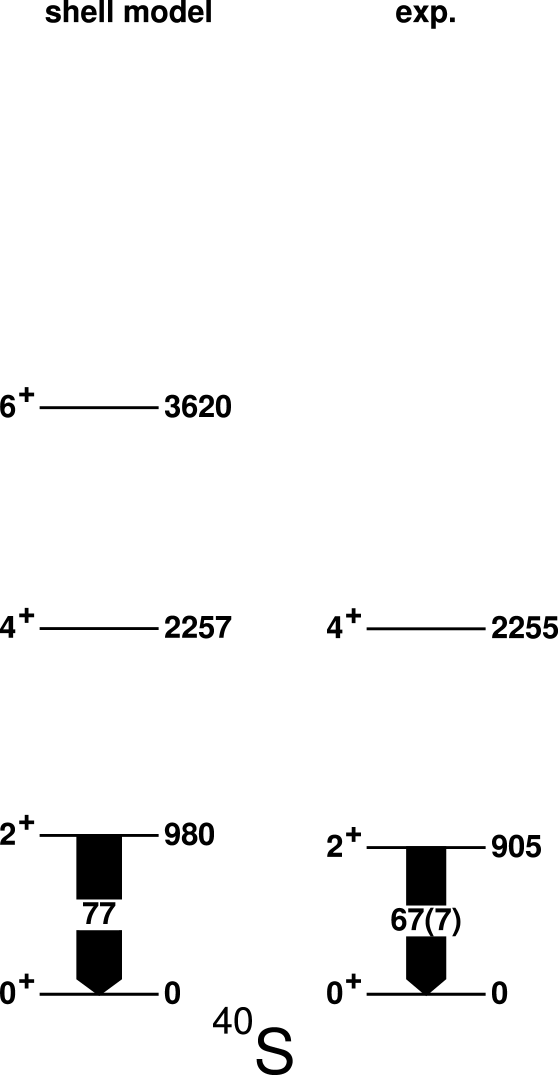
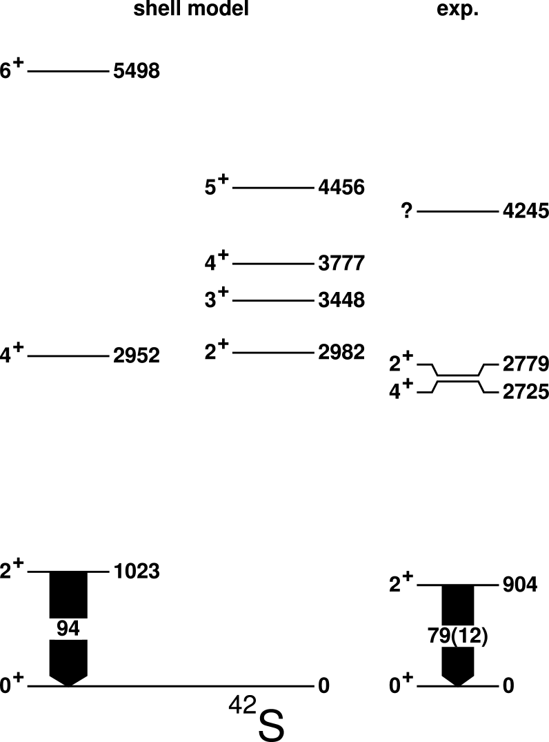
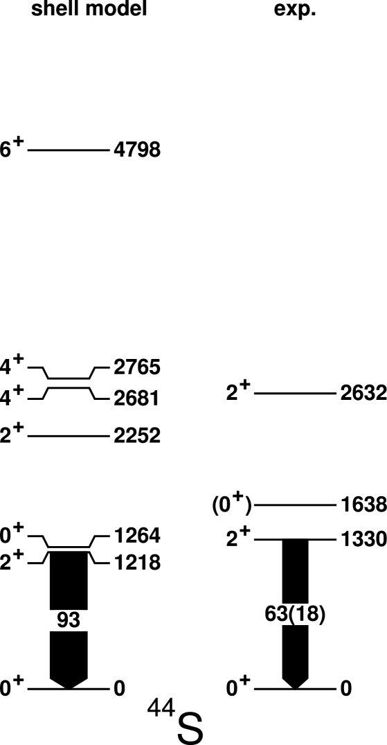
Figure 50: Predicted level schemes of the heavy sulphur isotopes, compared with the experiment. Energies in keV, B(E2)’s in e² fm⁴

In Fig. 50 we have plotted the low energy spectra of the heaviest known sulphur isotopes. The agreement with the accumulated experimental results (see Glasmacher, 1998, for a recent review) is excellent and extends to the new data of Sohler et al. (2002). Analyzing their proton occupancies we conclude that the rise in collectivity along the chain is correlated with the equal filling of the $d_{3/2}$ and $s_{1/2}$ orbitals, (the $d_{5/2}$ orbital remains always nearly closed). The maximum proton collectivity is achieved when both orbitals are degenerate, which corresponds to the Pseudo-SU(3) limit. For the neutrons, the maximum collectivity occurs at $N=24$, the $f_{7/2}$ mid-shell. According to the calculation, ⁴²S is a prolate rotor, with an incipient $\gamma$ band. In ⁴⁴S the spherical and deformed configurations mix equally.

The N=27 isotones also reflect the regular transition from sphericity to deformation in their low-lying spectrum. The excitation energy of the $3/2^{-}$ state should be sensitive to the correlations and to the neutron gap. While in ⁴⁷Ca, it lies quite high (at around 2 MeV) due to the strong $f_{7/2}$ closure, in ⁴⁵Ar it appears at about 0.4 MeV. Concerning ⁴³S, the information comes from two recent experiments: the mass measurements at Ganil by Sarazin et al. (2000) that observed a low-lying isomer around 400 keV excitation energy and the MSU Coulex experiment of Ibbotson et al. (1999) that detected a strong E2 transition from the ground state to an excited state around 940 keV. According to our calculations the ground state corresponds to the deformed configuration and has spin 3/2^-. The spherical single hole state 7/2^- would be the first excited state and his lifetime is consistent with that of the experimental isomer. The third known state is short lived and it should correspond to the 7/2^- member of the ground state band.

Table 14: N=28 isotones: Spectra, quadrupole properties and occupancies

	40Mg	42Si	44S	46Ar
E∗(2+)(MeV)	0.81	1.49	1.22	1.51
E∗(4+)	2.17	2.68	2.25	3.46
E∗(0${}^{+}_{2}$)	1.83	1.57	1.26	2.93
$Q(2^{+}$)(e fm2)	-21	16	-17	20
B(E2)(e2 fm4)	108	71	93	93
$\langle{n}_{7/2}\rangle$	5.54	6.16	6.16	6.91
$({f}_{7/2})^{8}$ %	3	28	24	45

VII.4 N=40; from “magic” ⁶⁸Ni to deformed ⁶⁴Cr

Systematics is a most useful guide, but it has to be used with care. The $p$ and $sd$ shells can be said to be “full” 0$\hbar\omega\,$ spaces, in the sense that the region boundaries are well defined by the $N=4$, 8 and $20$ closures, with the exception for the very neutron-rich halo nuclei and the island of inversion discussed previously. In the $pf$-shell it is already at $N=Z\approx 36$ that the 0$\hbar\omega\,$ model space collapses under the invasion of deformed intruders. Naturally, we expect something similar in the neighborhood of $N=40$ isotones. Recent experiments involving the Coulomb excitation of ^66-68Ni  Sorlin et al. (2002), the $\beta$ decay of ^60-63V  Sorlin et al. (2003), and the decay and the spectroscopy of the ^67mFe  Sawicka et al. (2003), support this hypothesis. In addition, the $\beta$ decays of the neutron-rich isotopes ⁶⁴Mn and ⁶⁶Mn, investigated at Isolde  Hannawald et al. (1999), that show a sudden drop of the $2^{+}$ energies in the daughter nuclei ⁶⁴Fe and ⁶⁶Fe, point also in the same direction.

In defining the new model spaces, the full $pf$ results are quite useful: ⁵⁶Ni turns out to be an extraordinarily good pivot (refer to Fig. 15), and as soon as a few particles are added it becomes a good core. Therefore, for the first time we are faced with a genuine EI space $r_{3}\,g_{9/2}$ (remember $r_{3}$ is the “rest” of the $p=3$ shell). Its validity is restricted to nearly spherical states. Deformation will demand the addition of the $d_{5/2}$ subshell.

Table 15: 2${}^{+}_{1}$ energies and $g_{9/2}$ intruder occupation in the Nickel isotopic chain, from  Sorlin et al. (2002)

	62Ni	64Ni	66Ni	68Ni	70Ni	72Ni	74Ni
E(2+)calc.	1.11	1.24	1.49	1.73	1.50	1.42	1.33
E(2+)exp.	1.173	1.346	1.425	2.033	1.259
B(E2$\uparrow$)calc.	775	755	520	265	410	505	690
$\langle{n}_{9/2}\rangle$	0.24	0.43	0.67	1.07	0.84	0.55	0.45

The effective interaction is based on three blocks: i) the TBME from KB3G effective interaction Poves et al. (2001), ii) the G-matrix of ref. Hjorth-Jensen et al. (1995) with the modifications of ref. Nowacki (1996) and iii) the Kahana, Lee and Scott G-matrix Kahana et al. (1969b) for the remaining matrix elements. We have computed all the nickel isotopes and followed their behavior at and beyond N=40. Let’s first focus on ⁶⁸Ni. The calculated low energy spectrum, an excited 0⁺ at 1.85 MeV, 2⁺ at 2.15 MeV, 5^- at 2.72 MeV and 4⁺ at 3.10 MeV, fit remarkably well with the experimental results. The ground state wave function is 50% closed shell. This number is very sensitive to modifications of the $pf$-$g$ gap, and smaller values of the closed shell probability can be obtained without altering drastically the rest of the properties. The SM results have been compared with those of other methods in Langanke et al. (2003b).

Table 16: Spectroscopic properties of ^60-64Cr in the $fpgd$ valence space

	60Cr	62Cr	64Cr
E∗(2+) (MeV)	0.67	0.65	0.51
Qs(e.fm2)	-23	-27	-31
B(E2)$\downarrow$(e2.fm4)	288	302	318
Qi(e.fm2) from Qs	82	76	109
Qi(e.fm2) from B(E2)	101	103	106
E∗(4+) (MeV)	1.43	1.35	1.15
Qs(e.fm2)	-37	-30	-43
B(E2)$\downarrow$(e2.fm4)	426	428	471
Qi(e.fm2) from Qs	102	84	119
Qi(e.fm2) from B(E2)	117	117	123

In table 15 we compare the excitation energy of the 2⁺ states in the Nickel chain with the available experimental data (including the very recent ⁷⁰Ni value Sorlin et al. (2002)). The agreement is quite good, although the experiment gives a larger peak at N=40. Similarly the B(E2)’s in Fig. 51 follow the experimental trends including the drop at ⁶⁸Ni recently measured Sorlin et al. (2002). Note that for a strict closure the transition would vanish.

Figure 51: B(E2) (0⁺ $\rightarrow$ 2⁺) in e² fm⁴ for the Nickel isotopes, from  Sorlin et al. (2002)

The $\beta$ decays of ⁶⁰V and ⁶²V indicate very low energies for the 2${}^{+}_{1}$ states in ⁶⁰Cr and ⁶²Cr Sorlin et al. (2000, 2003). If N=40 were a magic number, one would expect higher 2⁺ energies as the shell closure approaches, particularly in ⁶⁴Cr. As seen in Fig. 52, exactly the opposite seems to happen experimentally. The three possible model spaces tell an interesting story: $pf\equiv r_{3}$ is acceptable at $N=32,\,34$. The addition of $g_{9/2}$ does more harm than good because the gaps have been arbitrarily reduced to reproduce the $N=36$ experimental point by allowing 2p-2h jumps including $d_{5/2}$. But then, in $N=38$ the 2⁺ is too high, and the experimental trend promises no improvement at $N=40$.

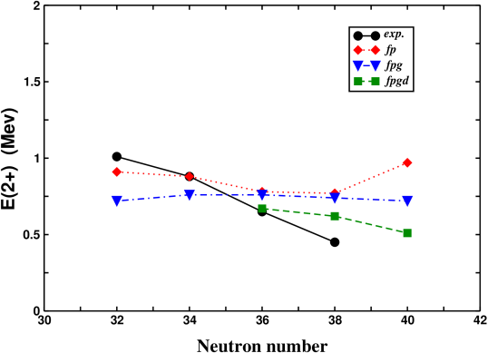
Figure 52: Experimental and calculated 2⁺ energies in the $pf$, $pfg$ and $pfgd$ spaces.

Properties of the 2${}^{+}_{1}$ energies given by the $pfgd$ calculation are collected in table 16. They point to prolate structures with deformation $\beta\approx 0.3$.

VIII Other regions and themes

VIII.1 Astrophysical applications

Astrophysical environments involve conditions of temperature and densities that are normally not accessible in laboratory experiments. The description of the different nuclear processes requires then theoretical estimates. As discussed in previous sections, shell-model calculations are able to satisfactorily reproduce many experimental results so that it should be possible to obtain reliable predictions for nuclei and/or conditions not yet accessible experimentally.

As a first example, consider the decay properties of nuclei totally stripped of the atomic electrons at typical cosmic rays energies of 300 MeV/A. A nucleus such as ⁵³Mn, unstable in normal conditions, becomes stable. Another isotope, ⁵⁴Mn, could be used as a chronometer to study the propagation of iron group nuclei on cosmic-rays Duvernois (1997) provided its half-life under cosmic-rays conditions is known. The necessary calculation involves decay by second-forbidden unique transitions to the ground states of ⁵⁴Cr and ⁵⁴Fe. Due to phase space arguments the $\beta^{-}$ decay to ⁵⁴Fe is expected to dominate. In two difficult and elegant experiments the very small branching ratio for the $\beta^{+}$ decay to the ground state of ⁵⁴Cr has been measured: $(1.8\pm 0.8)\times 10^{-9}$ by Zaerpoor et al. (1997) and $(1.20\pm 0.26)\times 10^{-9}$ by Wuosmaa et al. (1998). Taking the weighted mean of this values, $(1.26\pm 0.25)\times 10^{-9}$, and knowing that of ⁵⁴Mn, 312.3(4) d, a partial $\beta^{+}$ half-life of $(6.8\pm 1.3)\times 10^{8}$ yr is obtained compared with $5.6\times 10^{8}$ yr from the shell model calculation of Martínez-Pinedo and Vogel (1998), which yields $5.0\times 10^{5}$ yr for the dominant $\beta^{-}$ branch. Both theoretical results are sensitive to uncertainties in the renormalization of the unique second-forbidden operators that should be removed taking the ratio of the $\beta^{-}$ and $\beta^{+}$ half-lives. Multiplying the theoretical ratio by the experimental value of the $\beta^{+}$ half-life yields a value of $(6.0\pm 1.2)\times 10^{5}$ yr for the $\beta^{-}$ branch. Using a similar argument Wuosmaa et al. (1998) estimate the partial $\beta^{-}$ half-life to be $(6.0\pm 1.3[\mathrm{{stat}]\pm 1.1[\mathrm{theor}]})\times 10^{5}$. The influence of this half-life on the age of galactic cosmic-rays has been discussed recently by Yanasak et al. (2001). Another possible cosmic ray chronometer, ⁵⁶Ni, could measure the time between production of iron group nuclei in supernovae and the accelaration of part of this matterial to form cosmic rays Fisker et al. (1999). Before acceleration, the decay of ⁵⁶Ni proceeds by electron capture to the 1⁺ state in ⁵⁶Co with a half-live of 6.075(20) days. After acceleration ⁵⁶Ni is stripped of its electrons, the transition to the 1⁺ state is no longer energetically allowed and the decay proceeds to the 3⁺ state at 158 keV via a second forbidden unique transition. Currently only a lower limit for the half-life of totally ionized ⁵⁶Ni could be established ($2.9\times 10^{4}$ y) Sur et al. (1990). A recent shell-model calculation by Fisker et al. (1999) predict a half-live of $4\times 10^{4}$ y that is too short for ⁵⁶Ni to serve as a cosmic ray chronometer.

Nuclear beta-decay and electron capture are important during the late stages of stellar evolution (see Langanke and Martínez-Pinedo, 2003, for a recent review). At the relevant conditions in the star electron capture and $\beta$ decay are dominated by Gamow-Teller (and Fermi) transitions. Earlier determinations of the appropriate weak interaction rates were based in the phenomenological work of Fuller, Fowler, and Newman (1980); Fuller, Fowler, and Newman (1982a, b); Fuller, Fowler, and Newman (1985). The shell model makes it possible to refine these estimates. For the $sd$ shell nuclei, important in stellar oxygen and silicon burning, we refer to Oda et al. (1994). More recently, it has been possible to extend these studies to $pf$ shell nuclei relevant for the pre-supernova evolution and collapse Langanke and Martínez-Pinedo (2001, 2000); Caurier et al. (1999a). The astrophysical impact of the shell-model based weak interaction rates have been recently studied by Heger et al. (2001a, b)

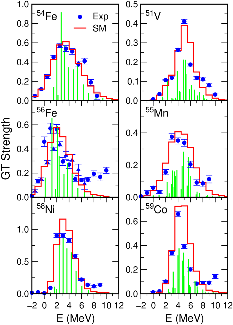
Figure 53: Comparison of shell model GT₊ distributions with experimental data Rönnqvist et al. (1993); El-Kateb et al. (1994); Alford et al. (1993) for selected nuclei. The shell model results (discrete lines) have been folded with the experimental resolution (histograms) and include a quenching factor of $(0.74)^{2}$ (adapted from Caurier et al., 1999a).

The basic ingredient in the calculation of the different weak interaction rates is the Gamow-Teller strength distribution. The GT₊ sector directly determines the electron capture rate and also contributes to the beta-decay rate through the thermal population of excited states Fuller et al. (1982a). The GT_- strength contributes to the determination of the $\beta$-decay rate. To be applicable to calculating stellar weak interaction rates the shell-model calculations should reproduce the available GT₊ (measured by $(n,p)$-type reactions) and GT_- (measured in $(p,n)$-type reactions). Figure 53 compares the shell-model $GT_{+}$ distributions with the pioneering measurements performed at TRIUMF. These measurements had a typical energy resolution of $\approx 1$ MeV. Recently developed techniques, involving $(d,{}^{2}\text{He})$ charge-exchange reactions at intermediate energies Rakers et al. (2002), have improved the energy resolution by an order of magnitude or more. Figure 54 compares the shell-model GT₊ distribution computed using the KB3G interaction Poves et al. (2001) with a recent experimental measurement of the ⁵¹V$(d,{}^{2}\text{He})$ performed at KVI Bäumer et al. (2003).

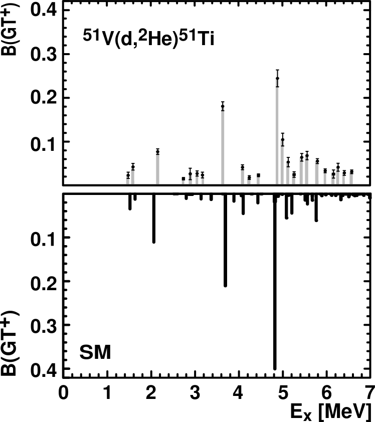
Figure 54: Comparison of the shell-model GT₊ distribution (lower panel) for ⁵¹V with the high resolution $(d,{}^{2}\text{He})$ data (from Bäumer et al., 2003). The shell-model distribution includes a quenching factor of $(0.74)^{2}$.

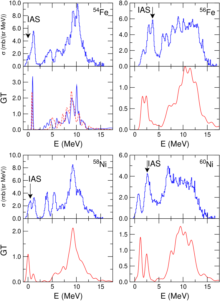
Figure 55: Comparison of $(p,n)$ $L=0$ forward angle cross section data Rapaport et al. (1983) (upper panels) with the calculated GT_- strength distributions (lower panels). For ⁵⁴Fe the solid curve in the lower panel shows the experimental GT_- data from Anderson et al. (1990), while the shell model results are given by the dashed line. The Fermi transition to the isobaric analog state (IAS) is included in the data (upper panels) but not in the calculations. A quenching factor of $(0.74)^{2}$ is included in the calculations. (from Caurier et al., 1999a).

Figure 55 compares the shell-model GT_- distributions with the data obtained in $(p,n)$ charge-exchange reaction measurements for ^54,56Fe and ^58,60Ni Rapaport et al. (1983); Anderson et al. (1990). The GT_- operator acting on a nucleus with neutron excess and ground state isospin $T$ can lead to states in the daughter nucleus with three different isospin values $(T-1,T,T+1)$. As a consequence, the GT_- strength distributions have significantly more structure and extend over a larger excitation energy interval than the GT₊ distributions, making their theoretical reproduction more challenging. Nevertheless, the agreement with the experimental data is quite satisfactory. The shell-model results for ⁵⁸Ni have been recently compared with high-resolution data (50 keV) obtained using the $({}^{3}\text{He},t)$ reaction Fujita et al. (2002).

Shell-model diagonalization techniques have been used to determine astrophysically relevant weak interaction rates for nuclei with $A\leq 65$. Nuclei with higher masses are relevant to study the collapse phase of core-collapse supernovae Langanke and Martínez-Pinedo (2003). The calculation of the relevant electron-capture rates is currently beyond the possibilities of shell-model diagonalization calculations due to the enormous dimensions of the valence space. However, this dimensionality problem does not apply to Shell-Model Monte-Carlo methods (SMMC, see section IV.2.3). Moreover, the high temperatures present in the astrophysical environment makes necessary a finite temperature treatment of the nucleus, this makes SMMC methods the natural choice for this type of calculations. Initial studies by Langanke et al. (2001) showed that the combined effect of nuclear correlations and finite temperature was rather efficient in unblocking Gamow-Teller transitions on neutron rich germanium isotopes. More recently this calculations have been extended to cover all the relevant nuclei in the range $A=65$–112 by Langanke et al. (2003a). The resulting electron-capture rates have a very strong influence in the collapse Langanke et al. (2003a) and post-bounce Hix et al. (2003)

The astrophysical r-process is responsible for the synthesis of at least half of the elements heavier than $A\approx 60$ Wallerstein et al. (1997). Simulations of the r-process require the knowledge of nuclear properties far from the valley of stability Kratz et al. (1998); Pfeiffer et al. (2001). As the relevant nuclei are not experimentally accessible, theoretical predictions for the relevant quantities (i.e., neutron separation energies and half-lives) are needed. The calculation of $\beta$ decay half-lives usually requires two ingredients: the Gamow-Teller strength distribution in the daughter nucleus and the relative energy scale between parent and daughter (i.e. the $Q_{\beta}$ value). Due to the huge number of nuclei relevant for the r process, the estimates of the half-lives are so far based on a combination of global mass models and the quasi particle random-phase approximation (see Langanke and Martínez-Pinedo, 2003, for a description of the different models). However, recently shell-model calculations have become available for some key nuclei with a magic neutron number $N=50$ Langanke and Martínez-Pinedo (2003), $N=82$ Brown et al. (2003); Martínez-Pinedo and Langanke (1999), and $N=126$ Martínez-Pinedo (2001). All this calculations suffer from the lack of spectroscopic information on the regions of interest that is necessary to fine tune the effective interactions. This situation is improving at least for $N=82$ thanks to the recent spectroscopic data on ¹³⁰Cd Dillmann et al. (2003).

Nuclear reaction rates are the key input data for simulations of stellar burning processes. Experiment-based reaction rates for the simulation of explosive processes such as novae, supernovae, x-ray bursts, x-ray pulsars, and merging neutron stars are scarce because of the experimental difficulties associated with radioactive beam measurements Käppeler et al. (1998). Most of the reaction rate tables are therefore based on global model predictions. The most frequently used model is the statistical Hauser Feshbach approach Rauscher and Thielemann (2000). For nuclei near the drip-lines or near closed shell configurations, the density of levels is not high enough for the Hauser Feshbach approach to be applicable. For these cases alternative theoretical approaches such as the nuclear shell model need to be applied. Shell-model calculations were used for the determination of the relevant proton capture reaction rates for $sd$-shell nuclei necessary for rp process studies Herndl et al. (1995). This calculations have been recently extended to include $pf$-shell nuclei Fisker et al. (2001).

Knowledge of neutrino nucleus reactions is necessary for many applications, e.g. the neutrino oscillation studies, detection of supernova neutrinos, description of the neutrino transport in supernovae and nucleosynthesis studies. Most of the relevant neutrino reactions have not been studied experimentally so far and their cross sections are typically based on nuclear theory (see Kolbe et al., 2003, for a recent review). The model of choice for the theoretical description of neutrino reactions depends of the energy of the neutrinos that participate in the reaction.

For low neutrino energies, comparable to the nuclear excitation energy, neutrino-nucleus reactions are very sensitive to the appropriate description of the nuclear response that is very sensitive to correlations among nucleons. The model of choice is then the nuclear shell-model. $0\hbar\omega$ calculations have been used for the calculation of neutrino absorption cross sections Sampaio et al. (2001) and scattering cross sections Sampaio et al. (2002) for selected $pf$ shell nuclei relevant for supernovae evolution. For lighter nuclei complete diagonalizations can be performed in larger model spaces, e.g. $4\hbar\omega$ calculations for ¹⁶O Haxton (1987); Haxton and Johnson (1990) and $6\hbar\omega$ calculations for ¹²C Hayes and Towner (2000); Volpe et al. (2000). Other examples of shell-model calculations of neutrino cross sections are the neutrino absorption cross sections on ⁴⁰Ar of Ormand et al. (1995) for solar neutrinos (see Bhattacharya et al., 1998, for an experimental evaluation of the same cross section), this cross section have been recently evaluated by Kolbe et al. (2003) for supernova neutrinos. And the evaluation by Haxton (1998) of the solar neutrino absorption cross section on ⁷¹Ga relevant for the GALLEX and SAGE solar neutrino experiments.

For higher neutrino energies the standard method of choice is the random phase approximation as the neutrino reactions are sensitive mainly to the total strength and energy centroids of the different multipoles contributing to the cross section. In some selected cases, the Fermi and Gamow-Teller contribution to the cross section could be determined from shell-model calculation that is supplemented by RPA calculations for higher multipoles. This type mix calculation has been carried out for several iron isotopes Kolbe et al. (1999); Toivanen et al. (2001) and for ²⁰Ne Heger et al. (2003).

VIII.2 $\beta\beta$-decays

The double beta decay is the rarest nuclear weak process. It takes place between two even-even isobars, when the decay to the intermediate nucleus is energetically forbidden or hindered by the large spin difference between the parent ground state and the available states in the intermediate nuclei. It comes in three forms: The two-neutrino decay $\beta\beta_{2\nu}$:

$${}^{A}_{Z}X_{N}\longrightarrow_{Z+2}^{A}X_{N-2}+e^{-}_{1}+e^{-}_{2}+\bar{\nu}_{1}+\bar{\nu}_{2}$$

is just a second order process mediated by the Standard model weak interaction It conserves the lepton number and has been already observed in a few nuclei.

The second mode, the neutrinoless decay $\beta\beta_{0\nu}$:

$${}^{A}_{Z}X_{N}\longrightarrow^{A}_{Z+2}X_{N-2}+e^{-}_{1}+e^{-}_{2}$$

needs an extension of the standard model of electroweak interactions as it violates lepton number. A third mode, $\beta\beta_{0\nu,\chi}$ is also possible

$${}^{A}_{Z}X_{N}\longrightarrow^{A}_{Z+2}X_{N-2}+e^{-}_{1}+e^{-}_{2}+\chi$$

in some extensions of the standard model and proceeds via emission of a light neutral boson, a Majoron $\chi$. The last two modes, not yet experimentally observed, require massive neutrinos –an issue already settled by the recent measures by Super-Kamiokande Fukuda et al. (1998), SNO Ahmad et al. (2002) and KamLAND Eguchi et al. (2003). Interestingly, the double beta decay without emission of neutrinos would be the only way to sign the Majorana character of the neutrino and to distinguish between the different scenarios for the neutrino mass differences. Experimentally, the three modes show different electron energy spectra ((see figure 2 in Zdesenko, 2002)), the $\beta\beta_{2\nu}$ and $\beta\beta_{0\nu,\chi}$ are characterized by a continuous spectrum ending at the maximum available energy $Q_{\beta\beta}$, while the $\beta\beta_{0\nu}$ spectrum consists in a sharp peak at the end of the $Q_{\beta\beta}$ spectrum. This should, in principle, make it easier the signature of this mode. In what follows we shall concentrate in the $\beta\beta_{2\nu}$ and $\beta\beta_{0\nu}$ modes.

The theoretical expression of the half-life of the 2$\nu$ mode can be written as:

$$[T^{2\nu}_{1/2}]^{-1}=G_{2\nu}|M^{2\nu}_{GT}|^{2},$$ (94)

with

$$M^{2\nu}_{GT}(J)=\sum_{m}\displaystyle{\frac{\langle J^{+}||\vec{\bm{\sigma}}t_{-}||1^{+}_{m}\rangle\langle 1^{+}_{m}||\vec{\bm{\sigma}}t_{-}||0^{+}\rangle}{E_{m}+E_{0}(J)}}$$ (95)

(there is an implicit sum over all the nucleons). $G_{2\nu}$ contains the phase space factors and the axial coupling constant $g_{A}$. The calculation of $M^{2\nu}_{GT}$ requires the precise knowledge of the ground state of the parent nuclei and the ground state and occasionally a few excited states of the grand daughter, both even-even. Besides, it is necessary to have a good description of the Gamow- Teller strength functions of both of them, which implies a detailed description of the odd-odd intermediate nucleus. This is why this calculation is a challenge for the nuclear models, and why agreement with the experiment in this channel is taken as a quality factor to be applied to the predictions of the models for the neutrinoless mode.

It is also a show-case of the use of the Lanczos strength function (LSF) method. It works as follows: Once the relevant wave functions of parent and grand daughter are obtained, it is straightforward to build the doorway states $\vec{\sigma}t_{-}|0^{+}_{initial}\rangle$ and $\vec{\sigma}t_{+}|J^{+}_{final}\rangle$. In a second step, one of them is fragmented using LSF, producing, at iteration N, N 1⁺ states in the intermediate nucleus, with excitation energies E_m. Overlapping these vectors with the other doorway, entering the appropriate energy denominators and adding up the N contributions gives an approximation to the exact value of $M^{2\nu}_{GT}$ (N=1 is just the closure approximation). Finally, the number of iterations is increased until full convergence is reached. The method is very efficient, for instance, in the A=48 case, 20 iterations suffice largely. The contributions of the different intermediate states to the final matrix element are plotted in Fig. 56.

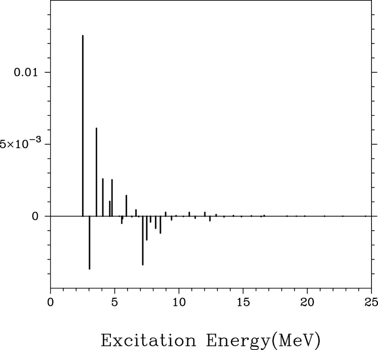
Figure 56: LSF for ⁴⁸Ca $\rightarrow$ ⁴⁸Ti 2$\nu$ decay. Each bar corresponds to a contribution to the matrix element. Notice the interfering positive and negative contributions.

In the $pf$-shell there is only one double beta emitter, namely ⁴⁸Ca. For many years, the experimental information was limited to a lower limit on the 2$\nu$-$\beta\beta$ half-life T${}^{2\nu}_{1/2}$$>$ 3.6$\times$10¹⁹ $yr$ Bardin et al. (1970). The calculation of the ⁴⁸Ca half-life was one of the first published results stemming from the full $pf$-shell calculations using the code ANTOINE. The resulting matrix elements are: $M^{2\nu}_{GT}(0^{+})$=0.083 and $M^{2\nu}_{GT}(2^{+})$=0.051. For the ground state to ground state decay ⁴⁸Ca$\rightarrow$⁴⁸Ti, G_2ν=1.1$\times$10^-17 $yr^{-1}$ Tsuboi et al. (1984). The phase space factor hinders the transition to the 2⁺ that represents only about 3% of the total probability. Putting everything together, and using the Gamow-Teller quenching factor, already discussed, the resulting half-life is T${}^{2\nu}_{1/2}$$=$ 3.7$\times$10¹⁹ $yr$, Caurier et al. (1990) (see also erratum in Caurier et al., 1994). The prediction was a success, because a later measure gave T${}^{2\nu}_{1/2}$$=$ 4.3${}^{+2.4}_{-1.1}$[stat]$\pm$1.4[syst] $\times$10¹⁹ $yr$ Balysh et al. (1996).

Among the other $\beta\beta$ emitters in nature (around 30), only a few are potentially interesting for experiment since they have a $Q_{\beta\beta}$ value, sufficiently large ($\geq 2.5MeV$) for the $0\nu$ signal not to be drowned in the surrounding natural radioactivity. With the exception of ¹⁵⁰Nd, all of them can be described within a shell model approach. The results for the $2\nu$ mode of the lightest emitters ⁴⁸Ca, ⁷⁶Ge and ⁸²Se, for which full space calculations are doable, are gathered in table LABEL:tab:2nu Caurier et al. (1996). The SMMC method has also been applied to the calculation of 2$\nu$ double beta decays in Radha et al. (1996).

Table 17: Calculated T${}_{1/2}^{2\nu}$ half-lives for several nuclei and $0^{+}\rightarrow 0^{+}$ transitions

Parent	${}^{48}Ca$	${}^{76}Ge$	${}^{82}Se$
$T_{1/2}^{2\nu}$ th.(y)	$3.7\times 10^{19}$	$2.6\times 10^{21}$	$3.7\times 10^{19}$
$T_{1/2}^{2\nu}$ exp.(y)	$4.3\times 10^{19}$	$1.8\times 10^{21}$	$8.0\times 10^{19}$

The expression for the neutrinoless beta decay half-life, in the $0^{+}\rightarrow 0^{+}$ case, can be brought to the following form Takasugi (1981); Doi et al. (1985):

$$[T_{1/2}^{(0\nu)}(0^{+}->0^{+}]^{-1}=$$

$$G_{0\nu}\left(M_{GT}^{(0\nu)}-\left(\frac{g_{V}}{g_{A}}\right)^{2}M_{F}^{(0\nu)}\right)^{2}\left(\frac{\langle m_{\nu}\rangle}{m_{e}}\right)^{2}$$

where $\langle m_{\nu}\rangle$ is the effective neutrino mass, $G_{0\nu}$ the kinematic space factor and M${}_{GT}^{(0\nu)}$ and M${}_{F}^{(0\nu)}$ the following matrix elements ($m$ and $n$ sum over nucleons):

$$M_{GT}^{(0\nu)}=\left<0_{f}^{+}\right\|\displaystyle\sum_{n,m}h(r)(\vec{\bm{\sigma}}_{n}\cdot\vec{\bm{\sigma}}_{m})t_{n\_}t_{m\_}\left\|0_{i}^{+}\right>$$ (96)

$$M_{F}^{(0\nu)}=\left<0_{f}^{+}\right\|\displaystyle\sum_{n,m}h(r)t_{n\_}t_{m\_}\left\|0_{i}^{+}\right>,$$ (97)

where, due to the presence of the neutrino propagator, the “neutrino potential” $h(r)$ is introduced. In this case, the matrix elements are just expectation values of two body operators, without a sum over intermediate states. This was believed to make the results less dependent of the nuclear model employed to obtain the wave function. An assumption that has not survived to the actual calculations. Full details of the calculations as well as predictions for other 0$\nu$ and 2$\nu$ decays in heavier double beta emitters can be found in Retamosa et al. (1995) and Caurier et al. (1996) (see also Suhonen and Civitarese, 1998, for a recent and very comprehensive review of the nuclear aspects of the double beta decay). The upper bounds on the neutrino mass resulting of our SM calculations, assuming a reference half-life T${}_{1/2}^{0\nu}\geq 10^{25}\;y.$ are collected in table LABEL:tab:0nu.

Table 18: 0$\nu$ matrix elements and upper bounds on the neutrino mass for T${}_{1/2}^{0\nu}\geq 10^{25}$ y. $\langle m_{\nu}\rangle$ in eV.

Parent	${}^{48}Ca$	${}^{76}Ge$	${}^{82}Se$
$M_{GT}^{0\nu}$	0.63	1.58	1.97
$M_{F}^{0\nu}$	-0.09	0.19	-0.22
$\langle m_{\nu}\rangle$	0.94	1.33	0.49

For the heavier emitters, some truncation scheme has to be employed and the seniority truncation seem to be the best, since the dimensions are strongly reduced in particular for 0⁺ states. An interesting feature in the calculation of the double beta decay matrix elements is shown in Fig. 57 for the ⁷⁶Ge case : the convergence of the $M_{GT}^{0\nu}$ matrix element is displayed as a function of the truncation of the valence space, either with the seniority $v$ or with the configurations $t$ (t is the maximum number of particles in the $g_{\frac{9}{2}}$ orbital). The $t=16$ and $v=16$ values correspond to the full space calculation and are consequently equal. The two truncation schemes show very distinct patterns, with the seniority truncation being more efficient. Such patterns have been also observed in the Tellurium and Xenon isotopes. This seems to indicate that the most favorable nuclei for the theoretical calculation of the $0\nu$ mode would be the spherical emitters, where seniority is an efficient truncation scheme.

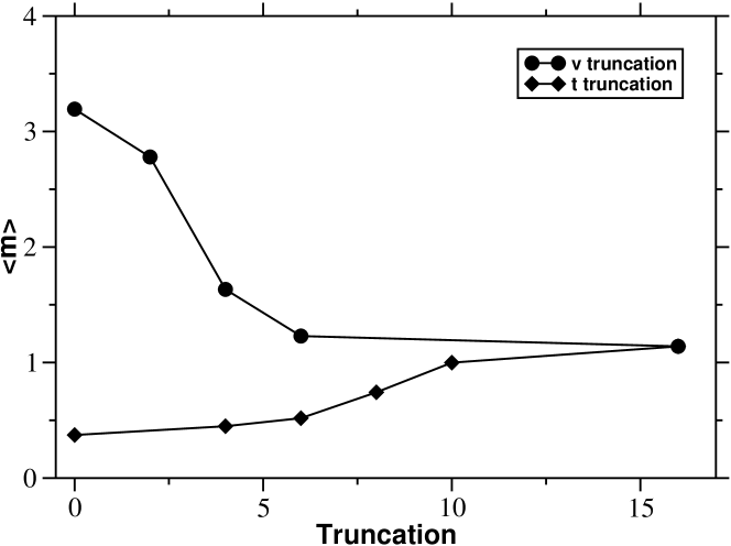
Figure 57: Variation of the $\langle m_{\nu}\rangle$ limit as a function of seniority truncations (circles) and configuration truncations (diamonds)

VIII.3 Radii isotope shifts in the Calcium isotopes

We have already seen in section VI.5 that deformed np-nh configurations can appear at very low excitation energy around shell closures and even to become yrast in the case of neutron rich nuclei. This situation simply reflects the limitation of the spherical mean field description of the nucleus, and shows that even in magic cases, the correlations produce a sizeable erosion of the Fermi surface. This is the case in the Calcium isotopic chain. Experiments based on optical isotope shifts or muonic atom data, reveal that the nuclear charge radii $\langle r_{c}^{2}\rangle$ follow a characteristic parabolic shape with a pronounced odd-even staggering  Fricke et al. (1995); Palmer (1984).

For the description of the nuclei around N=Z=20, a model space comprising the orbits 1d${}_{\frac{3}{2}}$, 2s${}_{\frac{1}{2}}$, 1f${}_{\frac{7}{2}}$ and 2p${}_{\frac{3}{2}}$ is a judicious choice (see Caurier et al., 2001a). The interaction is the same used to describe the neutron rich nuclei in the $sd$-$pf$ valence space, called sdpf.sm in section VII, with modified single particle energies to reproduce the spectrum of ²⁹Si.

Several important features of the nuclei at the $sd$/$pf$ interface are reproduced by the calculation, among others, the excitation energies of the intruder 0${}^{+}_{2}$ states in the Calcium isotopes as well as the location of the $\frac{3}{2}^{+}$ states in the Scandium isotopes (see Fig. 58), the excitation energies of the 2⁺ and 3^- and the B(E2)’s between the 2${}^{+}_{1}$ and the 0${}^{+}_{1}$ states in the Calcium isotopes.

Figure 58: Comparison between calculated and experimental intruder excitation energies in the Calcium and Scandium isotopic chains

Due to the cross shell pairing interaction, protons and neutrons are lifted from the $sd$ to the $fp$ orbitals. The former produce an increase of $\langle r^{2}_{c}\rangle$ that, using HO wave functions, can be expressed as:

$$\delta r^{2}_{c}(A)=\displaystyle\frac{1}{Z}n^{\pi}_{pf}(A)b^{2}$$ (98)

where Z=20 for the calcium chain, $b$ is the oscillator parameter, and $n^{\pi}_{pf}$ is extracted from the calculated wave functions. The charge radii isotope shifts of the Calcium isotopes relative to ⁴⁰Ca are shown in Fig. 59, together with the experimental values. The global trends are very well reproduced, although the calculated shifts are a bit smaller than the experimental ones. This is probably due to the limitations in the valence space, that excludes the 1d${}_{\frac{5}{2}}$, the 1f${}_{\frac{5}{2}}$ and the 2p${}_{\frac{1}{2}}$ orbits.

Figure 59: Isotopes shifts in Calcium chain: experimental (circles) versus shell model calculations (stars)

VIII.4 Shell model calculations in heavier nuclei

There are some regions of heavy nuclei in which physically sound valence spaces can be designed that are at the same time tractable. A good example is the space comprising the neutron orbits between N=50 and N=82 for the tin isotopes Hjorth-Jensen et al. (1995); Nowacki (1996). When protons are allowed the dimensions grow rapidly and the calculations have been limited until now to nuclei with few particle or holes on the top of the closed shells (see Covello et al., 1997, for a review of the work of the Napoli group).

The SMMC, that can overcome these limitations, has been applied in this region to ¹²⁸Te and ¹²⁸Xe that are candidates to $\gamma$ soft nuclei by Alhassid et al. (1996) and also to several Dysprosium isotopes A=152-162 in the Kumar-Baranger space by White et al. (2000). The QMCD method has been also applied to the study of the spherical to deformed transition in the even Barium isotopes with A=138-150 by Shimizu et al. (2001).

Hints on the location of the hypothetical islands of super heavy elements are usually inspired in mean-field calculations of the single particle structure. The predictions for nuclei far from stability can be tested also in nuclei much closer to stability, where shell model calculations are now feasible. In particular, recent systematic mean field calculations suggest a substantial gap for $Z=92$ and $N=126$ (²¹⁸U) corresponding to the 1h${}_{\frac{9}{2}}$ shell closure. On the other hand, the single quasiparticle energies extrapolated from lighter N=126 isotones up to ²¹⁵Ac, do not support this conclusion. To shed light on these controversial predictions, shell model calculations (as well as experimental spectroscopic studies of ²¹⁶Th  Hauschild et al. (2001)) were undertaken in the $N=126$ isotones up to ²¹⁸U. Shell model calculations were performed in the 1h${}_{\frac{9}{2}}$, 2f${}_{\frac{7}{2}}$, 1i${}_{\frac{13}{2}}$, 3p${}_{\frac{3}{2}}$, 2f${}_{\frac{5}{2}}$, 3p${}_{\frac{1}{2}}$ proton valence space, using the realistic Kuo-Herling interaction Kuo and Herling (1971) as modified by Brown and Warburton Warburton and Brown (1991). The calculation reproduces nicely the ground state energies, the 2⁺ energy systematics as well as the high-spin trends. The cases of ²¹⁴Ra, ²¹⁶Th and ²¹⁸U are shown in figure 60. The only deviations between theory and experiment are in the 3^- energy and reflect the particular nature of theses states which are known to be very collective and corresponding to particle hole excitations of the ²⁰⁸Pb core.

No shell gap for Z=92, corresponding to the 1h${}_{\frac{9}{2}}$ closure, is predicted. On the contrary, the ground state of the N=126 isotones is characteristic of a superfluid regime with seniority zero components representing more than 95% of the wave functions for all nuclei.

Figure 60: Experimental vs theoretical spectrum of ²¹⁴Ra, ²¹⁶Th, and ²¹⁸U

VIII.5 Random Hamiltonians

The study of random Hamiltonians is a vast interdisciplinary subject that falls outside the scope of this review (see Porter, 1965, for a collection of the pioneering papers). Therefore here we shall only give a bibliographical guide to work that has recently attracted wide attention and may have consequences in future shell model studies. Johnson et al. (1998, 1999) noticed that random interactions had a strong tendency to produce $J=0$ ground states. This is an empirical fact that was hitherto attributed to the pairing force. Bijker et al. (1999); Bijker and Frank (2000a, b) showed that in an interacting boson context this also occurred, and was associated to the typical forms of collectivity found in the IBM. For the fermion problem no collectivity occurs for purely random interactions Horoi et al. (2001). The origin of $J=0$ ground state-dominance was attributed to “geometric chaoticity” Mulhall et al. (2000). The geometric aspects of the phenomenon were investigated in some simple cases by Zhao and Arima (2001); Zhao et al. (2001) and Chau Huu-Tai et al. (2003). Velázquez and Zuker (2002) argued that the general cause of $J=0$ ground state-dominance was to be found in time-reversal invariance, and showed that when the random matrix elements were displaced to have a negative centroid, well developed rotational motion appeared in the valence spaces where the realistic interactions would also produce it (as in Fig. 39). This is very much in line with what was found by Cortes et al. (1982), and the interesting point is that the collective ingredient induced by the displacement of the matrix elements is the quadrupole force.

It is unlikely that we shall learn much more from purely random Hamiltonians. However, the interplay of random and collective interactions may deserve further study. In particular: We know that a monopole plus pairing Hamiltonian is a good approximation. Would it be a good idea to replace the rest of the interaction by a random one, instead of neglecting it?

IX Conclusion

Nuclei are idiosyncratic, especially the lighter ones, accessible to shell model treatment. Energy scales that are well separated in other systems (as vibrational and rotational states in molecules) do overlap here, leading to strong interplay of collective and single particle modes. Nonetheless, secular behavior—both in the masses and the spectra—eventually emerges and the $pf$ shell is the boundary region were rapid variation from nucleus to nucleus is replaced by smoother trends. As a consequence, larger calculations become associated with more transparent physics, and give hints on how to extend the shell model philosophy into heavier regions where exact diagonalizations become prohibitive. In this review we have not hesitated to advance some ideas on how this could be achieved, by suggesting some final solution to the monopole problem, and exploiting the formal properties of the Lanczos construction.

The shell model has been craft and science: one invented model spaces and interactions and forced them on the spectra. Sometimes it worked very well. Then one wondered why such a phenomenology succeeded, to discover that there was not so much phenomenology after all. It is to be hoped that this state of affairs will persist.

Appendix A Basic definitions and results

• $p$ is the principal oscillator quantum number

• $D_{p}=(p+1)(p+2)$ is the (single fluid) degeneracy of shell $p$

• Orbits are called $r$, $s$, etc. $D_{r}=2j_{r}+1$

• $\hat{\delta}_{rs}=\delta_{j_{r}j_{s}}$ but $r\neq s$, and both have the same parity.

• $m_{r}$ is the number of particles in orbit $r$, $T_{r}$ is used for both the isospin and the isospin operator. In neutron-proton ($np$) scheme, $m_{rx}$ specifies the fluid $x$. Alternatively we use $n_{r}$ and $z_{r}$.

• $V^{\Gamma}_{rstu}$ or $\mathcal{V}^{\Gamma}_{rstu}$ are two body matrix elements. $W^{\Gamma}_{rstu}$ is used after the monopole part has been subtracted.

A few equations have to exhibit explicitly angular momentum ($J$), and isospin ($T$) conservation. We use Bruce French’s notations French (1966): $\Gamma$ stands for $JT$. Then $(-1)^{\Gamma}=(-1)^{J+T}$, $[\Gamma]=(2J+1)(2T+1)$, and in general $F(\Gamma)=F(J)F(T)$. Also$(-1)^{r}=(-1)^{j_{r}+1/2}$, $[r]=2(2j_{r}+1)$. Expressions carry to neutron-proton formalism simply by dropping the isospin factor.

The one particle creation and anhilation operators

$$A_{rr_{z}}=a_{rr_{z}}^{\dagger}\qquad B_{rr_{z}}=\tilde{a}_{rr_{z}}=(-1)^{r+r_{z}}a_{r-r_{z}}\,.$$ (99)

can be coupled to quadratics in $A$ and $B$,

$$X_{\Gamma\Gamma_{z}}^{\dagger}(rs) = (A_{r}A_{s})^{\Gamma}_{\Gamma_{z}},\quad X_{\Gamma\Gamma_{z}}(rs)=(B_{r}B_{s})^{\Gamma}_{\Gamma_{z}},$$

$$\quad S^{\gamma}_{\gamma_{z}}(rt) = (A_{r}B_{t})^{\gamma}_{\gamma_{z}}.$$ (100)

$Z_{\Gamma\Gamma_{z}}^{\dagger}(rs)=(1+\delta_{rs})^{-1/2}X_{\Gamma\Gamma_{z}}^{\dagger}(rs)$ is the normalized pair operator and $Z_{\Gamma\Gamma_{z}}(rs)$ its Hermitian conjugate.

For reduced matrix elements we use Racah’s definition

$$<\alpha\alpha_{z}|P_{\gamma_{z}}^{\gamma}|\beta\beta_{z}>=$$ (101)

$$(-1)^{\alpha-\alpha_{z}}\begin{pmatrix}\alpha&\gamma&\beta\\ -\alpha_{z}&\gamma_{z}&\beta_{z}\end{pmatrix}\,<\alpha\parallel P^{\gamma}\parallel\beta>\,.$$

The normal and multipole representations of $H$ are obtained through the basic recoupling

$$-(X_{\Gamma}^{\dagger}(rs)X_{\Gamma}(tu))^{0}=-(-1)^{u+t-\Gamma}\left[\frac{\Gamma}{r}\right]^{1/2}\delta_{st}S_{ru}^{0}+\\ \sum_{\gamma}[\Gamma\gamma]^{1/2}(-1)^{s+t-\gamma-\Gamma}\begin{Bmatrix}r&s&\Gamma\\ u&t&\gamma\end{Bmatrix}(S_{rt}^{\gamma}S_{su}^{\gamma})^{0},$$ (102)

whose inverse is

$$(S_{rt}^{\gamma}S_{su}^{\gamma})^{0}=(-1)^{u-t+\gamma}\left[\frac{\gamma}{r}\right]^{1/2}\delta_{st}S_{ru}^{0}-$$ (103)

$$\sum_{\Gamma}[\Gamma\gamma]^{1/2}(-1)^{s+t-\gamma-\Gamma}\begin{Bmatrix}r&s&\Gamma\\ u&t&\gamma\end{Bmatrix}(X_{\Gamma}^{\dagger}(rs)X_{\Gamma}(tu))^{0}.$$

The “normal” representation of ${\cal V}$ is then

$${\cal V}=\sum_{r\leq s\,t\leq u,\Gamma}{\cal V}_{rstu}^{\Gamma}Z_{rs\Gamma}^{\dagger}\cdot Z_{tu\Gamma}=\\ -\sum_{(rstu)\Gamma}\xi_{rs}\xi_{tu}[\Gamma]^{1/2}{\cal V}_{rstu}^{\Gamma}(X_{rs\Gamma}^{\dagger}X_{tu\Gamma})^{0},$$ (104)

where we have used

$$\xi_{rs}=\begin{cases}(1+\delta_{rs})^{-1/2}&\text{if r$\leq$ s},\\ (1+\delta_{rs})^{1/2}/2&\text{if no restriction},\end{cases}$$ (105)

so as to have complete flexibility in the sums. According to (102), ${\cal V}$ can be transformed into the “multipole” representation

$${\cal V}=\sum_{(rstu)\gamma}\xi_{rs}\xi_{tu}\left[[\gamma]^{1/2}\omega_{rtsu}^{\gamma}(S_{rt}^{\gamma}S_{su}^{\gamma})^{0}\right.\\ \left.+\delta_{st}\hat{\delta}_{ru}[s]^{1/2}\omega_{russ}^{0}S_{ru}^{0}\right],$$ (106)

where (sum only over Pauli-allowed $\Gamma$)

$$\omega_{rtsu}^{\gamma}=\sum_{\Gamma}(-1)^{s+t-\gamma-\Gamma}\left\{\begin{array}[]{ccc}r&s&\Gamma\\ u&t&\gamma\end{array}\right\}W_{rstu}^{\Gamma}[\Gamma],$$ (107)

$$W_{rstu}^{\Gamma}=\sum_{\gamma}(-1)^{s+t-\gamma-\Gamma}\left\{\begin{array}[]{ccc}r&s&\Gamma\\ u&t&\gamma\end{array}\right\}\omega_{rtsu}^{\gamma}[\gamma].$$ (108)

Eq.(103) suggests an alternative to (106)

$${\cal V} = \sum_{(rstu)\gamma}\xi_{rs}\xi_{tu}[\gamma]^{1/2}\omega_{rstu}^{\gamma}$$

$$\times\left[(S_{rt}^{\gamma}S_{su}^{\gamma})^{0}-(-1)^{\gamma+r-s}\left[\frac{\gamma}{r}\right]^{1/2}\delta_{st}\hat{\delta}_{ru}S_{ru}^{0}\right],$$

where each term is associated with a pure two body operator.

Appendix B Full form of ${\cal H}_{m}$

If we were interested only in extracting the diagonal parts of the monopole Hamiltonian in $jt$ scheme, ${\cal H}_{mT}$, the solution would consist in calculating traces of ${\cal H}$, and showing that they can be written solely in terms of number and isospin operators. Before we describe the technique for dealing with the non diagonal parts of ${\cal H}_{mT}$ i.e. for generalizing to them the notion of centroid, some remarks on the interest of such an operation may be in order.

The full ${\cal H}_{m}$ contains all that is required for Hartree Fock (HF) variation, but it goes beyond. Minimizing the energy with respect to a determinantal state will invariably lead to an isospin violation because neutron and proton radii tend to equalize Duflo and Zuker (2002), which demands different orbits of neutrons and protons. Therefore, to assess accurately the amount of isospin violation in the presence of isospin-breaking forces we must ensure its conservation in their absence. More generally, a full diagonalization of ${\cal H}_{m}$ is of great intrinsic interest. Now, the technical details.

Define the generalized number and isospin operators

$$S_{rs}=\hat{\delta}_{rs}[r]^{1/2}S_{rs}^{00}\,,\qquad T_{rs}=\frac{1}{2}\hat{\delta}_{rs}[r]^{1/2}S_{rs}^{01}$$ (110)

which, for $\delta_{rs}=1$, reduce to $S_{rr}=n_{r},\;T_{rr}=T_{r}$. By definition ${\cal H}_{m}$ contains the two body quadratic forms in $S_{rs}$ and $T_{rs}$:

$$S_{rtsu}=\zeta_{rs}\zeta_{tu}(S_{rt}S_{su}-\delta_{st}S_{ru}),$$ (111a)

$$T_{rtsu}=\zeta_{rs}\zeta_{tu}(T_{rt}\cdot T_{su}-\frac{3}{4}\delta_{st}S_{ru}),$$ (111b)

which in turn become for $\delta_{rt}=\delta_{su}=1$, $m_{rs}$ and $T_{rs}$ in Eqs. (10a) and (10b)

It follows that the form of ${\cal H}_{mT}$ must be

$${\cal H}_{mT}={\cal K}+\sum_{all}(a_{rtsu}S_{rtsu}-b_{rtsu}T_{rtsu})\hat{\delta}_{rt}\hat{\delta}_{su},$$ (112)

where the sum is over all possible contributions. This is a special Hamiltonian containing only $\lambda=0$ terms. Transforming to the normal representation through Eq. (108)

$$\omega^{00} = \delta_{\lambda 0}\delta_{\tau 0}\Longrightarrow{\cal V}_{rstu}^{J0}={\cal V}_{rstu}^{J1}=[rs]^{-1/2}$$

$$\omega^{01} = \delta_{\lambda 0}\delta_{\tau 1}\Longrightarrow{\cal V}_{rstu}^{J0}=3[rs]^{-1/2}\,,{\cal V}_{rstu}^{J1}=-[rs]^{-1/2}$$

and therefore

$$S_{rtsu} = \sum_{\Gamma}Z_{rs\Gamma}^{\dagger}\cdot Z_{tu\Gamma}=$$

$$= \sum_{J}Z_{rsJ0}^{\dagger}\cdot Z_{tuJ0}+\sum_{J}Z_{rsJ1}^{\dagger}\cdot Z_{tuJ1}$$

$$-T_{rtsu}=\frac{3}{4}\sum Z_{rsJ0}^{\dagger}\cdot Z_{tuJ0}-\frac{1}{4}\sum Z_{rsJ1}^{\dagger}\cdot Z_{tuJ1}$$ (113b)

and inverting

$$\sum_{J}Z_{rsJ0}^{\dagger}\cdot Z_{tuJ0}=\frac{1}{4}(S_{rtsu}-4T_{rtsu})$$ (114a)

$$\sum_{J}Z_{rsJ1}^{\dagger}\cdot Z_{tuJ1}=\frac{1}{4}(3S_{rtsu}+4T_{rtsu}).$$ (114b)

When $j_{r}=j_{s}=j_{t}=j_{u}$ and $r\neq s$ and $t\neq u$, both $S_{rust}$, $T_{rust}$ and $S_{rtsu}$, $T_{rtsu}$ are present. They can be calculated from (114a) and (114b) by exchanging $t$ and $u$,

$$\sum Z_{rsJ0}^{\dagger}\cdot Z_{utJ0} = -\sum(-1)^{J}Z_{rsJ0}^{\dagger}\cdot Z_{tuJ0}=$$ (115a)

$$= \frac{1}{4}(S_{rust}-4T_{rust})$$

$$\sum Z_{rsJ1}^{\dagger}\cdot Z_{utJ1} = \sum(-1)^{J}Z_{rsJ1}^{\dagger}\cdot Z_{tuJ1}=$$ (115b)

$$= \frac{1}{4}(3S_{rust}+4T_{rust})$$

and by combining (114a), (114b), (115a) and (115b)

$$\sum_{J}Z_{rsJ0}^{\dagger}\cdot Z_{tuJ0}\frac{(1\pm(-1)^{J})}{2}=$$ (116a)

$$\frac{1}{8}((S_{rtsu}-4T_{rtsu})\mp(S_{rust}-4T_{rust}))$$

$$\sum_{J}Z_{rsJ1}^{\dagger}\cdot Z_{tuJ1}\frac{(1\pm(-1)^{J})}{2}=$$ (116b)

$$\frac{1}{8}((3S_{rtsu}+4T_{rtsu})\pm(3S_{rust}+4T_{rust}))$$

To write ${\cal H}_{mT}$ we introduce the notations

$$\Phi(P)=1-(1-\delta_{rs})(1-\delta_{tu}),$$ (117)

$$\Phi(e)\equiv(\hat{\delta}_{rs}-\delta_{rs})(\hat{\delta}_{tu}-\delta_{tu}),$$ (118)

So for $r=s$ or $t=u$, $\Phi(P)=1$ and for $j_{r}=j_{s}=j_{t}=j_{u}$ and $\Phi(P)=0$, $\Phi(e)=1$. Then

$${\cal H}_{mT}={\cal K}+$$

$$\sum_{\begin{subarray}{c}r\leq s\\ t\leq u\\ T,\rho=\pm\end{subarray}}\hat{\delta}_{rt}\hat{\delta}_{su}\left[(1-\Phi(e))\overline{\cal V}_{rstu}^{T}\Omega_{rstu}^{T}+\Phi(e)\overline{\cal V}_{rstu}^{\rho T}\Omega_{rstu}^{\rho T}\right]$$

$$\rho={\rm sign~{}}(-1)^{J},\quad\Omega_{rstu}^{T}=\sum_{J}Z_{rsJT}^{\dagger}\cdot Z_{tuJT}$$

$$\Omega_{rstu}^{\pm T}=\sum_{J}Z_{rsJT}^{\dagger}\cdot Z_{tuJT}\,\frac{(1\pm(-1)^{J})}{2}.$$ (119)

The values of the generalized centroids $\overline{\cal V}_{rstu}^{T}$ and $\overline{\cal V}_{\rho T}$ are determined by demanding that ${\cal H}-{\cal H}_{mT}={\cal H}_{M}$ contain no contributions with $\lambda=0$. In other words

$$W_{rstu}^{JT}={\cal V}_{rstu}^{JT}-$$

$$-\hat{\delta}_{rt}\hat{\delta}_{su}\left[(1-\Phi(e))\overline{\cal V}_{rstu}^{T}+\Phi(e)\overline{\cal V}_{rstu}^{\rho T}\right]\,,$$ (120)

must be such that $\omega_{rtsu}^{0\tau}=0$, and from Eq. (108)

$$\sum_{(J)}[J]W_{rstu}^{JT}=0\therefore\overline{\cal V}_{rstu}^{T}=\sum_{(J)}[J]{\cal V}_{rstu}^{JT}/\sum_{(J)}[J].$$ (121)

Applying this prescription to all the terms leads to (obviously $\hat{\delta}_{rt}\hat{\delta}_{su}=1$ in all cases)

$$\overline{\cal V}_{rstu}^{T}=\sum_{(J)}{\cal V}_{rstu}^{JT}[J]/\sum_{(J)}[J]$$

$$\sum_{(J)}[J]=\frac{1}{4}\;\frac{D_{r}(D_{s}+2\Phi(P)(-1)^{T})}{1+\Phi(P)}$$

$$\overline{\cal V}_{rstu}^{\pm T}=\sum_{J}{\cal V}_{rstu}^{JT}[J](1\pm(-1)^{J})/\sum_{J}[J](1\pm(-1)^{J})$$

$$\sum_{J}[J](1\pm(-1)^{J})=\frac{1}{4}\,D_{r}(D_{r}\mp 2)$$

$$D_{r}=[r],\quad\quad\Phi(e)=1,\;{\rm for~{}}\overline{\cal V}_{rstu}^{\pm T}\,.$$ (122)

Through eqs.(114a), (114b), (116a), and (116b) we can obtain the form of ${\cal H}_{mT}$ in terms of the monopole operators by regrouping the coefficients affecting each of them. To simplify the presentation we adopt the following convention

$$\left\{\begin{array}[]{llll}\alpha\equiv rstu&r\leq s,t\leq u,&\hat{\delta}_{rt}\hat{\delta}_{su}=1,&{\rm BUT}\\ S_{\alpha}=S_{rtsu},&S_{\bar{\alpha}}=S_{rust},&T_{\alpha}=T_{rtsu},&T_{\bar{\alpha}}=T_{rust},\end{array}\right.$$

then

$${\cal H}_{mT}={\cal K}+\sum_{\alpha}(1-\Phi(e))(a_{\alpha}S_{\alpha}+b_{\alpha}T_{\alpha})$$

$$+\Phi(e)(a_{\alpha}^{d}S_{\alpha}+b_{\alpha}^{d}T_{\alpha}+a_{\alpha}^{e}S_{\bar{\alpha}}+b_{\alpha}^{e}T_{\bar{\alpha}}),\,{\rm with}$$ (123a)

$$a_{\alpha}=\frac{1}{4}(3\bar{\cal V}^{1}_{\alpha}+\bar{\cal V}_{\alpha}^{0})$$

$$b_{\alpha}=\frac{1}{4}(\bar{\cal V}^{1}_{\alpha}-\bar{\cal V}_{\alpha}^{0})$$ (123b)

$$a_{\alpha}^{d}=\frac{1}{8}(3\bar{\cal V}_{\alpha}^{+1}+3\bar{\cal V}_{\alpha}^{-1}+\bar{\cal V}_{\alpha}^{+0}+\bar{\cal V}_{\alpha}^{-0})$$

$$a_{\alpha}^{e}=\frac{1}{8}(3\bar{\cal V}_{\alpha}^{+1}-3\bar{\cal V}_{\alpha}^{-1}-\bar{\cal V}_{\alpha}^{+0}+\bar{\cal V}_{\alpha}^{-0})$$

$$b_{\alpha}^{d}=\frac{1}{2}({3}\bar{\cal V}_{\alpha}^{+1}+{3}\bar{\cal V}_{\alpha}^{-1}-\bar{\cal V}_{\alpha}^{+0}-\bar{\cal V}_{\alpha}^{-0})$$

$$b_{\alpha}^{e}=\frac{1}{2}({3}\bar{\cal V}_{\alpha}^{+1}-\phantom{3}\bar{\cal V}_{\alpha}^{-1}+\bar{\cal V}_{\alpha}^{+0}-\bar{\cal V}_{\alpha}^{-0})$$ (123c)

B.1 Separation of ${\cal H}_{mnp}$ and ${\cal H}_{m0}$

In $j$ formalism ${\cal H}_{mnp}$ is ${\cal H}_{mT}$ under another guise: neutron and proton shells are differentiated and the operators $T_{rs}$ and $S_{rs}$ are written in terms of four scalars $S_{r_{x}s_{y}};\;\;x,y=n\;{\rm or}\;p$.

We may also be interested in extracting only the purely isoscalar contribution to ${\cal H}_{mT}$, which we call ${\cal H}_{m0}$. The power of French’s product notation becomes particularly evident here, because the form of both terms is identical. It demands some algebraic manipulation to find

$${\cal H}_{mnp}\;{\text{o}r}\;{\cal H}_{m0}={\cal K}+\sum_{\alpha}\biggl{[}\bar{\cal V}_{\alpha}S_{\alpha}(1-\Phi(e))+$$

$$+\frac{1}{2}((\bar{\cal V}_{\alpha}^{+}+\bar{\cal V}_{\alpha}^{-})S_{\alpha}+(\bar{\cal V}_{\alpha}^{-}-\bar{\cal V}_{\alpha}^{+})S_{\bar{\alpha}})\Phi(e)\biggr{]}$$ (124)

with

$$\overline{\cal V}_{rstu}=\sum_{(\Gamma)}{\cal V}_{rstu}^{\Gamma}[\Gamma]/\sum_{(\Gamma)}[\Gamma]$$

$$\sum_{(\Gamma)}[\Gamma]=D_{r}(D_{s}-\Phi(P))/(1+\Phi(P))$$

$$\overline{\cal V}_{rstu}^{\pm}=\sum_{\Gamma}{\cal V}_{rstu}[\Gamma](1\pm(-1)^{\Gamma+2r})\quad$$

$$\sum_{\Gamma}[\Gamma](1\pm(-1)^{\Gamma+2r})=D_{r}(D_{r}\mp(-1)^{2r})$$ (125)

Of course we must remember that for ${\cal H}_{mnp}$,

$D_{r}=2j_{r}+1,\;(-1)^{2r}=-1,\;\Gamma\equiv J,$ etc., while for ${\cal H}_{m0}$

$D_{r}=2(2j_{r}+1),\;(-1)^{2r}=+1,\;\Gamma\equiv JT$; etc.

It should be noted that ${\cal H}_{m0}$ is not obtained by simply discarding the $b$ coefficients in eqs.(123), because we can extract some $\gamma=$00 contribution from the $T_{\alpha}$ operators. The point will become quite clear when considering the diagonal contributions.

B.2 Diagonal forms of ${\cal H}_{m}$

We are going to specialize to the diagonal terms of ${\cal H}_{mT}$ and ${\cal H}_{mnp}$, which involve only ${\cal V}_{rsrs}^{\Gamma}$ matrix elements whose centroids will be called simply ${\cal V}_{rs}$ and ${\cal V}_{rs}^{T}$ (the overline in $\overline{\cal V}_{rstu}^{T}$ was meant to avoid confusion with possible matrix elements ${\cal V}_{rstu}^{1}$ or ${\cal V}_{rstu}^{0}$, it can be safely dropped now). Then (123) becomes Eq. (11) and (124) becomes

$${\cal H}_{mnp}^{d}\;or\;{\cal H}_{m0}^{d}={\cal K}+\sum_{r\leq s}{\cal V}_{rs}\,n_{r}(n_{s}-\delta_{rs})/(1+\delta_{rs})$$ (126)

We rewrite the relevant centroids incorporating explicitly the Pauli restrictions

$${\cal V}_{rs} = \frac{\sum_{\Gamma}{\cal V}_{rsrs}^{\Gamma}[\Gamma](1-(-1)^{\Gamma}\delta_{rs})}{D_{r}(D_{s}-\delta_{rs})}$$ (127a)

$${\cal V}_{rs}^{T} = \frac{4\sum_{J}{\cal V}_{rsrs}^{JT}[J](1-(-1)^{J+T}\delta_{rs})}{D_{r}(D_{s}+2\delta_{rs}(-1)^{T})}$$ (127b)

$$a_{rs} = \frac{1}{4}(3{\cal V}^{1}_{rs}+{\cal V}^{0}_{rs})={\cal V}_{rs}+\frac{3}{4}\,\frac{\delta_{rs}}{D_{r}-1}\,b_{rs}$$

$$b_{rs} = {\cal V}^{1}_{rs}-{\cal V}^{0}_{rs}$$ (127c)

The relationship between $a_{rs}$ and ${\cal V}_{rs}$ makes it possible to combine eqs. (11) and (126) in a single form

$${\cal H}_{m}^{d}={\cal K}+\sum\frac{1}{(1+\delta_{rs})}\biggl{[}{\cal V}_{rs}\,n_{r}(n_{s}-\delta_{rs})+$$

$$+b_{rs}\left(T_{r}\cdot T_{s}-\frac{3n_{r}\bar{n}_{r}}{4(D_{r}-1)}\delta_{rs}\right)\biggr{]}$$ (128)

in which now the $b_{rs}$ term can be dropped to obtain ${\cal H}_{m0}^{d}$ or ${\cal H}_{mnp}^{d}$.

In the np scheme each orbit $r$ goes into two $r_{n}$ and $r_{p}$ and the centroids can be obtained through ($x,y=n$ or $p$, $x\not=y$)

$${\cal V}_{r_{x}s_{y}} = \frac{1}{2}\left[{\cal V}_{rs}^{1}\left(1-\frac{2\delta_{rs}}{D_{r}}\right)+{\cal V}_{rs}^{0}\left(1+\frac{2\delta_{rs}}{D_{r}}\right)\right]$$

$${\cal V}_{r_{x}s_{x}} = {\cal V}_{rs}^{1}$$ (129)

Note that the diagonal terms depend on the representation: ${\cal H}_{mnp}^{d}\not={\cal H}_{mT}^{d}$ in general.

Appendix C The center of mass problem

What do you do about center of mass? is probably the standard question most SM practitioners prefer to ignore or dismiss. Even if we may be tempted to do so, there is no excuse for ignoring what the problem is, and here we shall explain it in sufficient detail, so as to dispel some common misconceptions.

The center of mass (CM) problem arises because in a many body treatment it is most convenient to work with $A$ coordinates and momenta while only $A-1$ of them can be linearly independent since the solutions cannot depend on the center of mass coordinate $R=(\sum_{i}r_{i})/\sqrt{A}$ or momentum $P=(\sum_{i}p_{i})/\sqrt{A}$. The way out is to impose a factorization of the wavefunctions into relative and CM parts: $\Phi(r_{1}\,r_{2}\,\ldots r_{A})=\Phi_{rel}\,\phi_{CM}$. The potential energy is naturally given in terms of relative values, and for the kinetic energy we should do the same by referring to the CM momentum,

$$\sum_{i}(p_{i}-\frac{P}{\sqrt{A}})^{2}=\sum_{i}p_{i}^{2}-P^{2}=\frac{1}{A}\sum_{ij}(p_{i}-p_{j})^{2},$$ (130)

and change accordingly ${\cal K}_{ij}$ in Eq. (2). As we are only interested in wavefunctions in which the center of mass is at rest (or in its lowest possible state), we can add a CM operator to the Hamiltonian ${\cal H}\Longrightarrow{\cal H}+\lambda(R^{2}+P^{2})$, and calling $r_{ij}=r_{i}-r_{j}$ we have

$$R^{2}+P^{2}=\sum_{i}(r_{i}^{2}+p_{i}^{2})-\frac{1}{A}\sum_{ij}(r_{ij}^{2}+p_{ij}^{2}),$$ (131)

so that upon diagonalization the eigenvalues will be of the form $E=E_{rel}+\lambda(N_{CM}+3/2)$, and it only remains to select the states with $N_{CM}$=0. We are taking for granted separation of CM and relative coordinates. Unfortunately, this happens only for spaces that are closed under the CM operator (131): for $N_{CM}$ to be a good quantum number the space must include all possible states with $N_{CM}$ oscillator quanta. The problem was raised by Elliott and Skyrme (1955) who initiated the study of “particle-hole” (ph) excitations on closed shells. They noted that acting with $R-iP$ on the IPM ground state of ¹⁶O ($|0\rangle$) leads to

$$\sqrt{\frac{1}{18}}(\bar{p}_{1}s_{1}-\sqrt{2}\bar{p}_{3}s_{1}-\sqrt{5}\bar{p}_{1}d_{3}+\bar{p}_{3}d_{3}+3\bar{p}_{3}d_{5})|0\rangle,$$ (132)

where $\bar{p}_{2j}$ removes a particle and $s_{1}$ or $d_{2j}$ add a particle on $|0\rangle$. As $R-iP$ has tensorial rank $J^{\pi}T=1^{-}0$, Eq. (132) is telling us that out of five possible $1^{-}0$ excitations, one is “spurious” and has to be discarded.

Assume now that we are interested in 2p2p excitations. They involve jumps of two oscillator quanta (2$\hbar\omega\,$) and the CM eigenstates $(R-iP)^{2}|0\rangle$ involve the operator in Eq. (132), but also jumps to other shells, of the type $\bar{s}\,p\bar{p}\,(sd)\equiv\bar{s}\,(sd)$ or $(\bar{sd})\,(pf)\bar{p}\,(sd)\equiv\bar{p}\,(pf)$. Therefore, as anticipated, relative-CM factorization can be achieved only by including all states involving a given number of oscillator quanta. The clean way to proceed is through complete $N$$\hbar\omega\,$spaces, discussed in Sections II.1.1 and III.6. The 0$\hbar\omega\,$and EI spaces are also free of problems (the latter because no 1$\hbar\omega\,$$1^{-}0$ states exist). It remains to analyze the EEI valence spaces, where CM spuriousness is always present but strongly suppressed because the main contributors to $R-iP$ –of the type $pj\Longrightarrow p+1j\pm 1$, with the largest $j$– are always excluded. Consider EEI(1)=$p_{1/2},\,d_{5/2},\,s_{1/2}$. The only possible 1$\hbar\omega\,$$1^{-}0$ state is $\bar{p}_{1}s_{1}$, which according to Eq. (132) accounts for $(1/18)\%=5.6\%$ of the spurious state. This apparently minor problem was unduly transformed into a serious one through a proposal by Gloeckner and Lawson (1974). It amounts to project CM spuriousness through the ${\cal H}\Longrightarrow{\cal H}+\lambda(R^{2}+P^{2})$ prescription in the EEI(1) space by identifying $R-iP\equiv\bar{p}_{1}s_{1}$. The procedure is manifestly incorrect, as was repeatedly pointed out (see for instance Whitehead et al., 1977) but the misconception persists. An interesting and viable alternative was put forward by Dean et al. (1999) in calculations with two contiguous major shells. Further work on the subject would be welcome.

References

- Abgrall et al. (1967a) Abgrall, Y., G. Baron, E. Caurier, and G. Monsonego, 1967a, Phys. Lett. 26B, 53.
- Abgrall et al. (1967b) Abgrall, Y., E. Caurier, and G. Monsonego, 1967b, Phys. Lett. 24B, 609.
- Abzouzi et al. (1991) Abzouzi, A., E. Caurier, and A. P. Zuker, 1991, Phys. Rev. Lett. 66, 1134.
- Ahmad et al. (2002) Ahmad, Q. R., R. C. Allen, T. C. Andersen, J. D. Anglin, J. C. Barton, E. W. Beier, M. Bercovitch, J. Bigu, S. Biller, R. A. Black, I. Blevis, R. J. Boardman, et al. (SNO), 2002, Phys. Rev. Lett. 89, 011301.
- Alford et al. (1993) Alford, W. P., B. A. Brown, S. Burzynski, A. Celler, D. Frekers, R. Helmer, R. Henderson, K. P. Jackson, K. Lee, A. Rahav, A. Trudel, and M. C. Vetterli, 1993, Phys. Rev. C 48, 2818.
- Alhassid et al. (1996) Alhassid, Y., G. F. Bertch, D. J. Dean, and S. E. Koonin, 1996, Phys. Rev. Lett. 77, 1444.
- Alhassid et al. (1994) Alhassid, Y., D. J. Dean, S. E. Koonin, G. Lang, and W. E. Ormand, 1994, Phys. Rev. Lett. 72, 613.
- Alhassid et al. (1999) Alhassid, Y., S. Liu, and H. Nakada, 1999, Phys. Rev. Lett. 83, 4265.
- Altshuler et al. (1997) Altshuler, B. L., Y. Gefenand, A. Kamenevand, and L. S. Levitov, 1997, Phys. Rev. Lett. 78, 2803.
- Anderson et al. (1985) Anderson, B. D., T. Chittrakarn, A. R. Baldwin, C. Lebo, R. Madey, P. C. Tandy, J. W. Watson, B. A. Brown, and C. C. Foster, 1985, Phys. Rev. C 31, 1161.
- Anderson et al. (1990) Anderson, B. D., C. Lebo, A. R. Baldwin, T. Chittrakarn, R. Madey, and J. W. Watson, 1990, Phys. Rev. C 41, 1474.
- Andreozzi et al. (2003) Andreozzi, F., N. Lo Iudice, and A. Porrino, 2003, to be published in Phys. Rev. C, eprint nucl-th/0307046.
- Arima (2001) Arima, A., 2001, Prog. Part. Nucl. Phys. 46, 119.
- Arima et al. (1969) Arima, A., M. Harvey, and K. Shimuzi, 1969, Phys. Lett. B 30, 517.
- Arima and Iachello (1975) Arima, A., and F. Iachello, 1975, Phys. Rev. Lett. 35, 1069.
- Aumann et al. (2001) Aumann, T., A. Navin, D. P. Balamuth, D. Bazin, B. Blank, B. A. Brown, J. E. Bush, J. A. Caggiano, B. Davids, T. Glasmacher, V. Guimaraẽs, P. G. Hansen, et al., 2001, Phys. Rev. Lett. 84, 35.
- Axel et al. (1949) Axel, O., J. H. D. Jensen, and H. E. Suess, 1949, Phys. Rev. 75, 1766.
- Axiotis (2000) Axiotis, M., 2000, private communication.
- Azaiez (1999) Azaiez, F., 1999, in Experimental Nuclear Physics in Europe, edited by B. Rubio, M. Lozano, and W. Gelletly, volume 495 of AIP Conf. Proc., p. 171.
- Balysh et al. (1996) Balysh, A., A. De Silva, V. I. Lebedev, K. Lou, M. K. Moe, M. A. Nelson, A. Piepke, A. Pronskiy, M. A. Vient, and P. Vogel, 1996, Phys. Rev. Lett. 77, 5186.
- Bambynek et al. (1977) Bambynek, W., H. Behrens, M. H. Chen, B. Crasemann, M. L. Fitzpatrick, K. W. D. Ledingham, H. Genz, M. Mutterer, and R. L. Intermann, 1977, Rev. Mod. Phys. 49, 77; 49, 961(E).
- Bansal and French (1964) Bansal, R. K., and J. B. French, 1964, Phys. Lett. 11, 145.
- Baranger and Kumar (1968) Baranger, M., and K. Kumar, 1968, Nucl. Phys. A 110, 490.
- Bardin et al. (1970) Bardin, R. K., P. J. Gollon, J. D. Ullman, and C. S. Wu, 1970, Nucl. Phys. A 158, 337.
- Bäumer et al. (2003) Bäumer, C., A. M. van den Berg, B. Davids, D. Frekers, D. De Frenne, E.-W. Grewe, P. Haefner, M. N. H. F. Hofmann, M. Hunyadi, E. Jacobs, B. J. A. Korff, K. Langanke, et al., 2003, Phys. Rev. C 68, 031303.
- Behrens and Bühring (1982) Behrens, H., and W. Bühring, 1982, Electron Radial Wave Functions and Nuclear Beta-decay (Clarendon, Oxford).
- Bender et al. (2003a) Bender, M., H. Flocard, and P.-H. Heenen, 2003a, arXiv:nucl-th/0305021.
- Bender et al. (2003b) Bender, M., P.-H. Heenen, and P. G. Reinhard, 2003b, Rev. Mod. Phys. 75, 121.
- Bennaceur et al. (1999) Bennaceur, K., F. Nowacki, J. Okolowicz, and M. Ploszajczak, 1999, Nucl. Phys. A 651, 289.
- Bennaceur et al. (2000) Bennaceur, K., F. Nowacki, J. Okolowicz, and M. Ploszajczak, 2000, Nucl. Phys. A 671, 203.
- Bentley et al. (1998) Bentley, M. A., C. D. O’Leary, A. Poves, G. Martínez-Pinedo, D. E. Appelbe, R. A. Bark, D. M. Cullen, S. Ertürk, and A. Maj, 1998, Phys. Lett. B 437, 243.
- Bentley et al. (1999) Bentley, M. A., C. D. O’Leary, A. Poves, G. Martínez-Pinedo, D. E. Appelbe, R. A. Bark, D. M. Cullen, S. Ertürk, and A. Maj, 1999, Phys. Lett. B 451, 445.
- Bentley et al. (2000) Bentley, M. A., S. J. Williams, D. T. Joss, C. D. O’Leary, A. M. Bruce, J. A. Cameron, P. Fallon, L. Frankland, W. Gelletly, C. J. Lister, G. Martínez-Pinedo, A. Poves, et al., 2000, Phys. Rev. C 62, 051303R.
- Bertsch and Hamamoto (1982) Bertsch, G. F., and I. Hamamoto, 1982, Phys. Rev. C 26, 1323.
- Bes and Sorensen (1969) Bes, D. R., and R. A. Sorensen, 1969, in Adv. Nuc. Phys., edited by M. Baranger and E. Vogt (Plenum Press, New York).
- Bethe (1936) Bethe, H. A., 1936, Phys. Rev. 50, 332.
- Bhattacharya et al. (1998) Bhattacharya, M., A. García, N. I. Kaloskamis, E. G. Adelberger, H. E. Swanson, R. Anne, M. Lewitowicz, M. G. Saint-Laurent, W. Trinder, C. Donzaud, D. Guillemaud-Mueller, S. Leenhardt, et al., 1998, Phys. Rev. C , 3677.
- Bijker and Frank (2000a) Bijker, R., and A. Frank, 2000a, Phys. Rev. Lett. 84, 420.
- Bijker and Frank (2000b) Bijker, R., and A. Frank, 2000b, Phys. Rev. C 62, 014303.
- Bijker et al. (1999) Bijker, R., A. Frank, and S. Pittel, 1999, Phys. Rev. C 60, 021302.
- Bloom (1984) Bloom, S. D. B., 1984, Prog. Part. Nucl. Phys. 11, 505.
- Bohr (1952) Bohr, A., 1952, Kgl. Dan. Vid. Sel. Mat. Fys. Med. 26, 14.
- Bohr and Mottelson (1953) Bohr, A., and B. R. Mottelson, 1953, Kgl. Dan. Vid. Sel. Mat. Fys. Med. 27, 16.
- Bohr and Mottelson (1969) Bohr, A., and B. R. Mottelson, 1969, Nuclear Structure, vol. I (Benjamin, New York).
- Bohr et al. (1958) Bohr, A., B. R. Mottelson, and D. Pines, 1958, Phys. Rev. 110, 936.
- Borcea et al. (2001) Borcea, R., J. Äystö, E. Caurier, P. Dendooven, J. Döringa, M. Gierlik, M.Górska, H.Grawe, M. Hellströ m, Z. Janas, A. Jokinen, M. Karny, et al., 2001, Nucl. Phys. A 695, 69.
- Borge et al. (1997) Borge, M. J. G., H. Fymbo, D. Guillemaud-Mueller, P. Hornshoj, F. Humbert, B. Jonson, T. E. Leth, G. Martínez-Pinedo, T. Nilsson, G. Nyman, A. Poves, I. Ramos-Lerate, et al., 1997, Phys. Rev. C 55, R8.
- Brandolini et al. (1998) Brandolini, F., S. M. Lenzi, D. R. Napoli, R. V. Rivas, H. Somacal, C. A. Ur, D. Bazzacco, A. C. J, G. de Angelis, M. de Poli, C. Fahlander, A. Gadea, et al., 1998, Nucl. Phys. A 642, 387.
- Brandolini et al. (2002a) Brandolini, F., N. Marginean, S. Hankonen, N. H. Medina, R. V. Rivas, J. Sánchez Solano, S. M. Lenzi, S. Lunardi, D. R. Napoli, A. Poves, C. A. Ur, D. Bazzacco, et al., 2002a, Phys. Rev. C 66, 024304.
- Brandolini et al. (1999) Brandolini, F., N. H. Medina, S. M. Lenzi, D. R. Napoli, A. Poves, R. V. Rivas, J. Sánchez Solano, C. A. Ur, D. Bucurescu, M. De Poli, R. Menegazzo, D. Bazzacco, et al., 1999, Phys. Rev. C 60, 041305.
- Brandolini et al. (2001) Brandolini, F., N. H. Medina, R. V. Rivas, S. M. Lenzi, , A. Gadea, C. A. Ur, D. Bazzacco, R. Menegazzo, P. Pavan, C. Rossi-Alvarez, A. Algora-Pineda, et al., 2001, Phys. Rev. C 64, 044307.
- Brandolini et al. (2002b) Brandolini, F., J. Sánchez Solano, S. M. Lenzi, N. H. Medina, A. Poves, C. A. Ur, D. Bazzacco, G. de Angelis, M. De Poli, E. Farnea, A. Gadea, D. R. Napoli, et al., 2002b, Phys. Rev. C 66, 021302.
- Brown (2001) Brown, B. A., 2001, Prog. Part. Nucl. Phys. 47, 517.
- Brown et al. (2003) Brown, B. A., R. Clement, H. Schatz, J. Giansiracusa, W. A. Richter, M. Hjorth-Jensen, K. L. Kratz, B. Pfeiffer, and W. B. Walters, 2003, Nucl. Phys. A 719, 177c.
- Brown et al. (1985) Brown, B. A., A. Etchegoyen, W. D. M. Rae, N. S. Godwin, W. A. Richter, C. H. Zimmerman, W. E. Ormand, and J. S. Winfield, 1985, OXBASH code, Technical Report 524, MSU-NSCL.
- Brown et al. (1974) Brown, B. A., D. B. Fossan, J. M. McDonald, and K. A. Snover, 1974, Phys. Rev. C 9, 1033.
- Brown and Wildenthal (1988) Brown, B. A., and B. H. Wildenthal, 1988, Annu. Rev. Nucl. Part. Sci. 38, 29.
- Brueckner (1954) Brueckner, K., 1954, Phys. Rev. 96, 508.
- Cameron et al. (1991) Cameron, J. A., M. A. Bentley, A. M. Bruce, R. A. Cunningham, W. Gelletly, H. G. Price, J. Simpson, D. D. Warner, and A. N. James, 1991, Phys. Rev. C 44, 1882.
- Cameron et al. (1994) Cameron, J. A., M. A. Bentley, A. M. Bruce, R. A. Cunningham, W. Gelletly, H. G. Price, J. Simpson, D. D. Warner, and A. N. James, 1994, Phys. Rev. C 49, 1347.
- Cameron et al. (1993) Cameron, J. A., M. A. Bentley, A. M. Bruce, R. A. Cunningham, H. G. Price, J. Simpson, D. D. Warner, A. N. James, W. Gelletly, and P. V. Isacker, 1993, Phys. Lett. B 319, 58.
- Campi et al. (1975) Campi, X., H. Flocard, A. K. Kerman, and S. Koonin, 1975, Nucl. Phys. A 251, 193.
- Carter et al. (1964) Carter, E. B., G. E. Mitchell, and R. H. Davis, 1964, Phys. Rev. 133, 1421.
- Caurier et al. (1995a) Caurier, E., J. L. Egido, G. Martínez-Pinedo, A. Poves, J. Retamosa, L. M. Robledo, and A. P. Zuker, 1995a, Phys. Rev. Lett. 75, 2466.
- Caurier et al. (1999a) Caurier, E., K. Langanke, G. Martínez-Pinedo, and F. Nowacki, 1999a, Nucl. Phys. A 653, 439.
- Caurier et al. (2001a) Caurier, E., K. Langanke, G. Martínez-Pinedo, F. Nowacki, and P. Vogel, 2001a, Phys. Lett. B 522, 240.
- Caurier et al. (1999b) Caurier, E., G. Martínez-Pinedo, F. Nowacki, A. Poves, J. Retamosa, and A. P. Zuker, 1999b, Phys. Rev. C 59, 2033.
- Caurier et al. (1999c) Caurier, E., G. Martínez-Pinedo, F. Nowacki, A. Poves, J. Retamosa, and A. P. Zuker, 1999c, Nucl. Phys. A 164, 747c, proceedings INPC/98, B. Frois editor.
- Caurier et al. (2001b) Caurier, E., P. Navrátil, W. E. Ormand, and J. P. Vary, 2001b, Phys. Rev. C 64, 051301(R).
- Caurier et al. (2002) Caurier, E., P. Navrátil, W. E. Ormand, and J. P. Vary, 2002, Phys. Rev. C 66, 024314.
- Caurier and Nowacki (1999) Caurier, E., and F. Nowacki, 1999, Acta Physica Polonica 30, 705.
- Caurier et al. (2001c) Caurier, E., F. Nowacki, and A. Poves, 2001c, Nucl. Phys. A 693, 374.
- Caurier et al. (1996) Caurier, E., F. Nowacki, A. Poves, and J. Retamosa, 1996, Phys. Rev. Lett. 77, 1954.
- Caurier et al. (1998) Caurier, E., F. Nowacki, A. Poves, and J. Retamosa, 1998, Phys. Rev. C 58, 2033.
- Caurier et al. (1990) Caurier, E., A. Poves, and A. P. Zuker, 1990, Phys. Lett. B 252, 13.
- Caurier et al. (1995b) Caurier, E., A. Poves, and A. P. Zuker, 1995b, Phys. Rev. Lett. 74, 1517.
- Caurier et al. (2003) Caurier, E., M. Rejmund, and H. Grawe, 2003, Phys. Rev. C 67, 054310.
- Caurier et al. (1994) Caurier, E., A. P. Zuker, A. Poves, and G. Martínez-Pinedo, 1994, Phys. Rev. C 50, 225.
- Cavedon et al. (1982) Cavedon, J. M., J. B. Frois, D. Goutte, , M. Huet, P. Leconte, C. Papanicolas, X. H. Pham, S. Platchkov, S. Williamson, W. Boeglin, and I. Sick, 1982, Phys. Rev. Lett. 49, 978.
- Chau Huu-Tai et al. (2003) Chau Huu-Tai, P., A. Frank, N. A. Smirnova, and P. Van Isacker, 2003, arXiv:nucl-th/0301061.
- Chevallier et al. (1967) Chevallier, P., F. Scheibling, G. Goldring, I. Plesser, and M. W. Sachs, 1967, Phys. Rev. 160, 827.
- Chiara et al. (2003) Chiara, C. J., E. Ideguchi, M. Devlin, D. R. LaFosee, F. Lerma, W. Reviol, S. K. Yu, D. G. Sarantites, C. Backtash, A. Galindo-Uribarri, M. P. Carpenter, R. V. F. Janssens, et al., 2003, Phys. Rev. C 67, 041303.
- Chou et al. (1993) Chou, W.-T., E. K. Warburton, and B. A. Brown, 1993, Phys. Rev. C 47, 163.
- Coester and Kümmel (1960) Coester, F., and H. Kümmel, 1960, Nucl. Phys. 17, 477.
- Cohen and Kurath (1965) Cohen, S., and D. Kurath, 1965, Nucl. Phys. 73, 1.
- Cortes et al. (1982) Cortes, A., R. U. Haq, and A. P. Zuker, 1982, Phys. Lett. B 115, 1.
- Covello et al. (1997) Covello, A., F. Andreozzi, L. Coraggio, A. Gargano, T. T. S. Kuo, and A. Porrino, 1997, Prog. Part. Nucl. Phys. 18, 165.
- Dang et al. (1997) Dang, N. D., A. Arima, T. Suzuki, and S. Yamaji, 1997, Nucl. Phys. A 621, 719.
- Davidson (1975) Davidson, E. R., 1975, J. Comp. Phys. 17, 87.
- Dean et al. (1995) Dean, D. J., S. E. Koonin, K. Langanke, P. B. Radha, and Y. Alhassid, 1995, Phys. Rev. Lett. 74, 2009.
- Dean et al. (1999) Dean, D. J., M. T. Russell, M. Hjorth-Jensen, S. E. Koonin, K. Langanke, and A. P. Zuker, 1999, Phys. Rev. C 59, 2474.
- Dechargé and Gogny (1980) Dechargé, J., and D. Gogny, 1980, Phys. Rev. C 21, 1568.
- Descouvemont (2002) Descouvemont, P., 2002, Nucl. Phys. A 709, 275.
- Detraz et al. (1979) Detraz, C., D. Guillemaud, G. Huber, R. Klapisch, M. de Saint-Simon, C. Thibault, and F. Touchard, 1979, Phys. Rev. C 19, 164.
- Dillmann et al. (2003) Dillmann, I., K.-L. Kratz, A. Wöhr, O. Arndt, B. A. Brown, P. Hoff, M. Hjorth-Jensen, U. Köster, A. N. Ostrowski, B. Pfeiffer, D. Seweryniak, J. Shergur, et al., 2003, Phys. Rev. Lett. 91, 162503.
- Doi et al. (1985) Doi, M., T. Kotani, and E. Takasugi, 1985, Prog. Theor. Phys. Suppl. 83, 1.
- Drożdż et al. (1986) Drożdż, S., V. Klemt, J. Speth, and J. Wambach, 1986, Phys. Lett. B 166, 18.
- Duflo and Zuker (1995) Duflo, J., and A. P. Zuker, 1995, Phys. Rev. C 52, R23.
- Duflo and Zuker (1999) Duflo, J., and A. P. Zuker, 1999, Phys. Rev. C 59, R2347.
- Duflo and Zuker (2002) Duflo, J., and A. P. Zuker, 2002, Phys. Rev. C 66, 051303(R).
- Dufour and Zuker (1996) Dufour, M., and A. P. Zuker, 1996, Phys. Rev. C 54, 1641.
- Dukelsky and Pittel (2001) Dukelsky, J., and S. Pittel, 2001, Phys. Rev. C 63, 061303.
- Dukelsky et al. (2002) Dukelsky, J., S. Pittel, S. S. Dimitrova, and M. V. Stoistov, 2002, Phys. Rev. C 65, 054319.
- Duvernois (1997) Duvernois, M. A., 1997, Astrophys. J. 481, 241.
- Eguchi et al. (2003) Eguchi, K., S. Enomoto, K. Furuno, J. Goldman, H. Hanada, H. Ikeda, K. Ikeda, K. Inoue, K. Ishihara, W. Itoh, T. Iwamoto, T. Kawaguchi, et al. (KamLAND), 2003, Phys. Rev. Lett. 90, 021802.
- El-Kateb et al. (1994) El-Kateb, S., K. P. Jackson, W. P. Alford, R. Abegg, R. E. Azuma, B. A. Brown, A. Celler, D. Frekers, O. Haeusser, R. Helmer, R. S. Henderson, K. H. Hicks, et al., 1994, Phys. Rev. C 49, 3128.
- Elliott (1958a) Elliott, J. P., 1958a, Proc. Roy. Soc. London , 128.
- Elliott (1958b) Elliott, J. P., 1958b, Proc. Roy. Soc. London , 562.
- Elliott et al. (1968) Elliott, J. P., A. D. Jackson, H. A. Mavromantis, E. A. Sanderson, and B. Sing, 1968, Nucl. Phys. A 121, 241.
- Elliott and Lane (1957) Elliott, J. P., and A. M. Lane, 1957, in Handbuch der Physik XXXIX (Springer Verlag, Berlin).
- Elliott and Skyrme (1955) Elliott, J. P., and T. H. R. Skyrme, 1955, Proc. Roy. Soc. London A 232, 561.
- Endt and van der Leun (1990) Endt, P. M., and C. van der Leun, 1990, Nucl. Phys. A 521, 1.
- Entem and Machleidt (2002) Entem, D. R., and R. Machleidt, 2002, Phys. Lett. B 524, 93.
- Entem et al. (2002) Entem, D. R., R. Machleidt, and H. Witala, 2002, Phys. Rev. C 65, 064005.
- Fiase et al. (1988) Fiase, J., A. Hamoudi, J. M. Irvine, and F. Yazici, 1988, J. Phys G 14, 27.
- Firestone (1996) Firestone, R. B., 1996, Table of Isotopes (Wiley, New York).
- Fisker et al. (2001) Fisker, J. L., V. Barnard, J. Görres, K. Langanke, G. Martínez-Pinedo, and M. C. Wiescher, 2001, At. Data. Nucl. Data Tables 79, 241.
- Fisker et al. (1999) Fisker, J. L., G. Martínez-Pinedo, and K. Langanke, 1999, Eur. Phys. J. A 5, 229.
- French (1966) French, J. B., 1966, in Enrico Fermi Lectures XXXVI, edited by C. Bloch (Academic Press, New York).
- French (1969) French, J. B., 1969, in Isospin in Nuclear Physics, edited by D. H. Wilkinson (North Holland, Amsterdam).
- French et al. (1969) French, J. B., E. C. Halbert, J. B. McGrory, and S. S. M. Wong, 1969, in Adv. Nuc. Phys., edited by M. Baranger and E. Vogt (Plenum Press, New York), p. 193.
- Fricke et al. (1995) Fricke, G., C. Bernhardt, K. Heilig, L. A. Schaller, L. Schellenberg, E. B. Shera, and C. W. D. Jager, 1995, At. Data Nucl. Data Tables 60, 177.
- Fujita et al. (2002) Fujita, Y., H. Fujita, T. Adachi, G. P. A. Berg, E. Caurier, H. Fujimura, K. Hara, K. Hatanaka, Z. Janas, J. Kamiya, T. Kawabata, K. Langanke, et al., 2002, Eur. Phys. J. A 13, 411.
- Fukuda et al. (1998) Fukuda, Y., T. Hayakawa, E. Ichihara, K. Inoue, K. Ishihara, H. Ishino, Y. Itow, T. Kajita, J. Kameda, S. Kasuga, K. Kobayashi, Y. Kobayashi, et al. (Super-Kamiokande), 1998, Phys. Rev. Lett. 81, 1562.
- Fukunishi et al. (1992) Fukunishi, N., T. Otsuka, and T. Sebe, 1992, Phys. Lett. B 296, 279.
- Fuller et al. (1980) Fuller, G. M., W. A. Fowler, and M. J. Newman, 1980, Astrophys. J. Suppl. 42, 447.
- Fuller et al. (1982a) Fuller, G. M., W. A. Fowler, and M. J. Newman, 1982a, Astrophys. J. 252, 715.
- Fuller et al. (1982b) Fuller, G. M., W. A. Fowler, and M. J. Newman, 1982b, Astrophys. J. Suppl. 48, 279.
- Fuller et al. (1985) Fuller, G. M., W. A. Fowler, and M. J. Newman, 1985, Astrophys. J. 293, 1.
- Garrett et al. (2001) Garrett, P. E., W. E. Ormand, D. Appelbe, R. W. Bauer, J. A. Becker, L. A. Bernstein, J. A. Cameron, M. P. Carpenter, R. V. F. Janssens, C. J. Lister, D. Seweryniak, E. Tavukcu, et al., 2001, Phys. Rev. Lett. 87, 132502.
- Glasmacher (1998) Glasmacher, T., 1998, Annu. Rev. Nucl. Part. Sci. 48, 1.
- Gloeckner and Lawson (1974) Gloeckner, D., and R. Lawson, 1974, Phys. Lett. 53B, 313.
- Guillemaud-Mueller et al. (1984) Guillemaud-Mueller, D., C. Detraz, M. Langevin, F. Naulin, M. de Saint-Simon, C. Thibault, F. Touchard, and M. Epherre, 1984, Nucl. Phys. A 426, 37.
- Hagiwara et al. (2002) Hagiwara, K., K. Hikasa, K. Nakamura, M. Tanabashi, M. Aguilar-Benitez, C. Amsler, R. Barnett, P. Burchat, C. Carone, C. Caso, G. Conforto, O. Dahl, et al. (Particle Data Group), 2002, Phys. Rev. D 66, 010001, URL http://pdg.lbl.gov.
- Halbert et al. (1971) Halbert, E. C., J. B. McGrory, B. H. Wildenthal, and S. Pandya, 1971, in Adv. Nuc. Phys., edited by M. Baranger and E. Vogt (Plenum Press, New York).
- Hannawald et al. (1999) Hannawald, M., T. Kautsch, A. Wöhr, W. Walters, K.-L. Kratz, V. N. Fedoseyev, V. I. Mishin, W. Böhmer, B. Pfeiffer, V. Sebastian, Y. Jading, U. Köster, et al., 1999, Phys. Rev. Lett. 82, 1391.
- Hansen and Jonson (1987) Hansen, P. G., and B. Jonson, 1987, Europhysics Lett. 4, 409.
- Hara and Sun (1995) Hara, K., and Y. Sun, 1995, Int. J. Mod. Phys. E 4, 637.
- Hara et al. (1999) Hara, K., Y. Sun, and T. Mizusaki, 1999, Phys. Rev. Lett. 83, 1922.
- Hauschild et al. (2001) Hauschild, K., M. Rejmund, and H. Grawe, 2001, Phys. Rev. Lett. 87, 072501.
- Haxton (1987) Haxton, W. C., 1987, Phys. Rev. D 36, 2283.
- Haxton (1998) Haxton, W. C., 1998, Phys. Lett. B 431, 110.
- Haxton and Johnson (1990) Haxton, W. C., and C. Johnson, 1990, Phys. Rev. Lett. 65, 1325.
- Hayes and Towner (2000) Hayes, A. C., and I. S. Towner, 2000, Phys. Rev. C 61, 044603.
- Hecht and Adler (1969) Hecht, K. T., and A. Adler, 1969, Nucl. Phys. A A137, 129.
- Heger et al. (2003) Heger, A., E. Kolbe, W. Haxton, K. Langanke, G. Martínez-Pinedo, and S. E. Woosley, 2003, submitted to Phys. Rev. Lett., eprint astro-ph/0307546.
- Heger et al. (2001a) Heger, A., K. Langanke, G. Martínez-Pinedo, and S. E. Woosley, 2001a, Phys. Rev. Lett. 86, 1678.
- Heger et al. (2001b) Heger, A., S. E. Woosley, G. Martínez-Pinedo, and K. Langanke, 2001b, Astrophys. J. 560, 307.
- Heisenberg and Mihaila (2000) Heisenberg, J. H., and B. M. Mihaila, 2000, Phys. Rev. C 59, 1440.
- Herndl et al. (1995) Herndl, H., J. Görres, M. Wiescher, B. A. Brown, and L. van Wormer, 1995, Phys. Rev. C 52, 1078.
- Heyde and Woods (1991) Heyde, K., and J. L. Woods, 1991, J. Phys. G 17, 135.
- Hix et al. (2003) Hix, W. R., O. E. B. Messer, A. Mezzacappa, M. Liebendörfer, J. Sampaio, K. Langanke, D. J. Dean, and G. Martínez-Pinedo, 2003, Phys. Rev. Lett. 91, 201102.
- Hjorth-Jensen (1996) Hjorth-Jensen, M., 1996, private communication to APZ.
- Hjorth-Jensen et al. (1995) Hjorth-Jensen, M., T. T. S. Kuo, and E. Osnes, 1995, Phys. Repts. 261, 126.
- Honma et al. (1996) Honma, M., T. Mizusaki, and T. Otsuka, 1996, Phys. Rev. Lett. 77, 3315.
- Honma et al. (2002) Honma, M., T. Otsuka, B. A. Brown, and T. Mizusaki, 2002, Phys. Rev. C 65, 061301.
- Horoi et al. (2001) Horoi, M., B. A. Brown, and V. Zelevinsky, 2001, Phys. Rev. Lett. 87, 062501.
- Horoi et al. (2002) Horoi, M., B. A. Brown, and V. Zelevinsky, 2002, Phys. Rev. C 65, 027303.
- Horoi et al. (2003) Horoi, M., B. A. Brown, and V. Zelevinsky, 2003, Phys. Rev. C 67, 034303.
- Horoi et al. (1999) Horoi, M., A. Volya, and V. Zelevinsky, 1999, Phys. Rev. Lett. 82, 2064.
- Iachello and Arima (1987) Iachello, F., and A. Arima, 1987, The interacting boson model (Cambridge University Press, Cambridge).
- Ibbotson et al. (1999) Ibbotson, R. W., T. Glasmacher, P. F. Mantica, and H. Scheit, 1999, Phys. Rev. C 59, 642.
- Ichimura and Arima (1966) Ichimura, M., and A. Arima, 1966, Prog. Theor. Phys. 36, 296.
- Id Betan et al. (2002) Id Betan, R., R. J. Liotta, N. Sandulescu, and T. Vertse, 2002, Phys. Rev. Lett. 89, 042501.
- Ideguchi et al. (2001) Ideguchi, E., D. G. Sarantites, W. Reviol, A. V. Afanasiev, M. Devlin, C. Baktash, R. V. F. Janssens, D. Rudolph, A. Axelsson, M. P. Carpenter, A. Galindo-Uribarri, D. R. LaFosse, et al., 2001, Phys. Rev. Lett. 87, 222501.
- Ikeda et al. (1963) Ikeda, K. I., S. Fujii, and J. I. Fujita, 1963, Phys. Lett. 3, 271.
- Iljinov et al. (1992) Iljinov, A. S., M. V. Mebel, N. Bianchi, E. de Sanctis, C. Guaraldo, V. Lucherini, V. Muccifora, E. Polli, A. R. Reolon, and P. Rossi, 1992, Nucl. Phys. A A543, 517.
- Iwasaki et al. (2001) Iwasaki, H., T. Motobayashi, H. Sakurai, K. Yoneda, T. Gomi, N. Aoi, N. Fukuda, , Z. Fülöp, U. Futakami, Z. Gacsi, Y. Higurashi, et al., 2001, Phys. Lett. B 522, 227.
- Janssens et al. (2002) Janssens, R. V. F., B. Fornal, P. F. Mantica, B. A. Brown, R. Broda, P. Bhattacharyya, M. P. Carpenter, M. Cinausero, P. J. Daly, A. D. Davies, T. Glasmacher, Z. W. Grabowski, et al., 2002, Phys. Lett. B 546, 55.
- Jiang et al. (1989) Jiang, M. F., R. Machleidt, D. B. Stout, and T. T. S. Kuo, 1989, Phys. Rev. C 40, 1857.
- Johnson et al. (1998) Johnson, C. W., G. F. Bertsch, and D. J. Dean, 1998, Phys. Rev. Lett. 80, 2749.
- Johnson et al. (1999) Johnson, C. W., G. F. Bertsch, D. J. Dean, and I. Talmi, 1999, Phys. Rev. C 61, 014311.
- Juodagalvis and Åberg (1998) Juodagalvis, A., and S. Åberg, 1998, Phys. Lett. B 428, 227.
- Kahana et al. (1969a) Kahana, S., H. Lee, and C. Scott, 1969a, Phys. Rev. 180, 956.
- Kahana et al. (1969b) Kahana, S., H. Lee, and C. Scott, 1969b, Phys. Rev. 185, 1378.
- Käppeler et al. (1998) Käppeler, F., F.-K. Thielemann, and M. Wiescher, 1998, Annu. Rev. Nucl. Part. Sci. 48, 175.
- Kawarada and Arima (1964) Kawarada, H., and A. Arima, 1964, J. Phys. Soc. Japan 19, 1768.
- Klotz et al. (1993) Klotz, G., P. Baumann, M. Bounajma, A. Huck, A. Knipper, G. Walter, G. Marguier, C. Richard-Serre, A. Poves, and J. Retamosa, 1993, Phys. Rev. C 47, 2502.
- Kolbe et al. (1999) Kolbe, E., K. Langanke, and G. Martínez-Pinedo, 1999, Phys. Rev. C 60, 052801.
- Kolbe et al. (2003) Kolbe, E., K. Langanke, G. Martínez-Pinedo, and P. Vogel, 2003, J. Phys. G: Nucl. Part. Phys. 29, 2569.
- Koonin et al. (1997a) Koonin, S. E., D. J. Dean, and K. Langanke, 1997a, Phys. Repts. 278, 2.
- Koonin et al. (1997b) Koonin, S. E., D. J. Dean, and K. Langanke, 1997b, Ann. Rev. Nucl. Part. Sci. 47, 463.
- Kratz et al. (1998) Kratz, K.-L., B. Pfeiffer, and F.-K. Thielemann, 1998, Nucl. Phys. A 630, 352.
- Kumar and Baranger (1968) Kumar, K., and M. Baranger, 1968, Nucl. Phys. A 110, 529.
- Kümmel et al. (1978) Kümmel, H. K., K. H. Lührmann, and J. G. Zabolitzky, 1978, Phys. Rep. 36, 1.
- Kuo and Brown (1968) Kuo, T. T. S., and G. Brown, 1968, Nucl. Phys. A 114, 241.
- Kuo and Brown (1966) Kuo, T. T. S., and G. E. Brown, 1966, Nucl. Phys. A 85, 40.
- Kuo and Herling (1971) Kuo, T. T. S., and G. H. Herling, 1971, NRL Memorandum Report 2258.
- Lanczos (1950) Lanczos, C., 1950, J. Res. Nat. Bur. Stand. 45, 252.
- Langanke (1998) Langanke, K., 1998, Phys. Lett. B 438, 235.
- Langanke et al. (1995) Langanke, K., D. J. Dean, P. B. Radha, Y. Alhasid, and S. E. Koonin, 1995, Phys. Rev. C 52, 718.
- Langanke et al. (2001) Langanke, K., E. Kolbe, and D. J. Dean, 2001, Phys. Rev. C 63, 032801.
- Langanke and Martínez-Pinedo (2000) Langanke, K., and G. Martínez-Pinedo, 2000, Nucl. Phys. A 673, 481.
- Langanke and Martínez-Pinedo (2001) Langanke, K., and G. Martínez-Pinedo, 2001, At. Data. Nucl. Data Tables 79, 1.
- Langanke and Martínez-Pinedo (2003) Langanke, K., and G. Martínez-Pinedo, 2003, Rev. Mod. Phys. 75, 819.
- Langanke et al. (2003a) Langanke, K., G. Martínez-Pinedo, O. E. B. Messer, J. M. Sampaio, D. J. Dean, W. R. Hix, A. Mezzacappa, M. Liebendörfer, H.-T. Janka, and M. Rampp, 2003a, Phys. Rev. Lett. 90, 241102.
- Langanke et al. (2003b) Langanke, K., J. Terasaki, F. Nowacki, D. J. Dean, and W. Nazarewicz, 2003b, Phys. Rev. C 67, 044314.
- Lawson and Macfarlane (1965) Lawson, R. D., and M. H. Macfarlane, 1965, Nuc. Phys. A 66, 80.
- Lee (1969) Lee, H. C., 1969, code made available to APZ.
- Lenzi et al. (2001) Lenzi, S. M., N. Marginean, D. R. Napoli, C. A. Ur, A. P. Zuker, G. de Angelis, A. Algora, M. Axiotis, D. Bazzacco, N. Belcari, M. A. Bentley, P. G. Bizzeti, et al., 2001, Phys. Rev. Lett. 87, 122501.
- Lenzi et al. (1996) Lenzi, S. M., D. R. Napoli, A. Gadea, M. A. Cardona, D. Hojman, M. A. Najarajan, C. Rossi-Alvarez, N. H. Medina, G. de Angelis, D. Bazzacco, M. E. Debray, M. De Poli, et al., 1996, Z. Phys. A 354, 117.
- Lenzi et al. (1999) Lenzi, S. M., D. R. Napoli, C. A. Ur, D. Bazzacco, F. Brandolini, J. A. Cameron, E. Caurier, G. de Angelis, M. De Poli, E. Farnea, A. Gadea, S. Hankonen, et al., 1999, Phys. Rev. C 60, 021303.
- Lenzi et al. (1997) Lenzi, S. M., C. A. Ur, D. R. Napoli, M. A. Najarajan, D. Bazzacco, D. M. Brink, M. A. Cardona, G. de Angelis, M. De Poli, A. Gadea, D. Hojman, S. Lunardi, et al., 1997, Phys. Rev. C 56, 1313.
- Long and Sun (2001) Long, G.-L., and Y. Sun, 2001, Phys. Rev. C 63, 021305.
- Machleidt (2001) Machleidt, R., 2001, Phys. Rev. C 63, 024001.
- Machleidt et al. (1996) Machleidt, R., F. Sammaruca, and Y. Song, 1996, Phys. Rev. C 53, R1483.
- Mantica et al. (2003) Mantica, P. F., A. C. Morton, B. A. Brown, A. D. Davis, T. Glasmacher, D. E. Groh, S. N. Liddick, D. J. Morrisey, W. F. Muelle, H. Schatz, A. Stolz, S. L. Tabor, et al., 2003, Phys. Rev. C 67, 014311.
- Marsden et al. (2002) Marsden, D. C. J., P. Navrátil, S. A. Coon, and B. R. Barrett, 2002, Phys. Rev. C 66, 044007.
- Martínez-Pinedo (2001) Martínez-Pinedo, G., 2001, Nucl. Phys. A 688, 357c.
- Martínez-Pinedo and Langanke (1999) Martínez-Pinedo, G., and K. Langanke, 1999, Phys. Rev. Lett. 83, 4502.
- Martínez-Pinedo et al. (1996a) Martínez-Pinedo, G., A. Poves, E. Caurier, and A. P. Zuker, 1996a, Phys. Rev. C 53, R2602.
- Martínez-Pinedo et al. (1996b) Martínez-Pinedo, G., A. Poves, L. M. Robledo, E. Caurier, F. Nowacki, J. Retamosa, and A. P. Zuker, 1996b, Phys. Rev. C 54, R2150.
- Martínez-Pinedo and Vogel (1998) Martínez-Pinedo, G., and P. Vogel, 1998, Phys. Rev. Lett. 81, 281.
- Martínez-Pinedo et al. (1997) Martínez-Pinedo, G., A. P. Zuker, A. Poves, and E. Caurier, 1997, Phys. Rev. C 55, 187.
- Mayer (1949) Mayer, M., 1949, Phys. Rev. 75, 1969.
- Mazzocchi et al. (2001) Mazzocchi, C., Z. Janas, J. Döring, M. Axiotis, L. Batist, R. Borcea, D. Cano-Ott, E. Caurier, G. de Angelis, E. Farnea, A. Faßbender, A. Gadea, et al., 2001, Eur. Phys. J. A 12, 269.
- McCullen et al. (1964) McCullen, J. D., B. F. Bayman, and L. Zamick, 1964, Phys. Rev. 134, 515.
- Michel et al. (2002) Michel, N., W. Nazarevicz, M. Ploszajczak, and K.Bennaceur, 2002, Phys. Rev. Lett. 89, 042502.
- Michel et al. (2003) Michel, N., W. Nazarevicz, M. Ploszajczak, and J. Okolowicz, 2003, Phys. Rev. C 67, 054311.
- Mihaila and Heisenberg (2000) Mihaila, B. M., and J. H. Heisenberg, 2000, Phys. Rev. C 61, 054309.
- Mizusaki (2000) Mizusaki, T., 2000, RIKEN Accel. Prog. Rep. 33, 14.
- Mizusaki and Imada (2002) Mizusaki, T., and M. Imada, 2002, Phys. Rev. C 65, 064319.
- Mizusaki and Imada (2003) Mizusaki, T., and M. Imada, 2003, Phys. Rev. C 67, 041301.
- Mizusaki et al. (2001) Mizusaki, T., T. Otsuka, M. Honma, and B. A. Brown, 2001, Phys. Rev. C 63, 044306.
- Mizusaki et al. (2002) Mizusaki, T., T. Otsuka, M. Honma, and B. A. Brown, 2002, Nucl. Phys. A 704, 190c.
- Mizusaki et al. (1999) Mizusaki, T., T. Otsuka, Y. Utsuno, M. Honma, and T. Sebe, 1999, Phys. Rev. C 59, 1846.
- Mon and French (1975) Mon, K. K., and J. B. French, 1975, Ann. Phys. (NY) 95, 90.
- Motobayashi et al. (1995) Motobayashi, T., Y. Ikeda, Y. Ando, K. Ieki, M. Inoue, N. Iwasa, T. Kikuchi, M. Kurokawa, S. Moriya, S. Ogawa, H. Murakami, S. Shimoura, et al., 1995, Phys. Lett. B 346, 9.
- Mulhall et al. (2000) Mulhall, D., A. Volya, and V. Zelevinsky, 2000, Phys. Rev. Lett. 85, 4916.
- Nakada and Alhassid (1997) Nakada, H., and Y. Alhassid, 1997, Phys. Rev. Lett. 79, 2939.
- Navin et al. (2000) Navin, A., D. W. Anthony, T. Aumann, T. Baumann, B. D, Y. Blumenfeld, B. A. Brown, T. Glasmacher, P. G. Hansen, R. W. Ibbotson, P. A. Lofy, V. Maddalena, et al., 2000, Phys. Rev. Lett. 85, 266.
- Navrátil and Barrett (1996) Navrátil, P., and B. R. Barrett, 1996, Phys. Rev. C 54, 2986.
- Navrátil and Barrett (1998) Navrátil, P., and B. R. Barrett, 1998, Phys. Rev. C 57, 562.
- Navrátil and Barrett (1999) Navrátil, P., and B. R. Barrett, 1999, Phys. Rev. C 59, 1906.
- Navrátil et al. (2000) Navrátil, P., G. P. Kamuntavičious, and B. R. Barrett, 2000, Phys. Rev. C 61, 044001.
- Navrátil and Ormand (2002) Navrátil, P., and W. E. Ormand, 2002, Phys. Rev. Lett. 88, 152502.
- Navrátil et al. (2001) Navrátil, P., W. E. Ormand, J. P. Vary, and B. R. Barrett, 2001, Phys. Rev. Lett. 87, 172502.
- Navrátil et al. (2000a) Navrátil, P., J. P. Vary, and B. R. Barrett, 2000a, Phys. Rev. Lett. 84, 5728.
- Navrátil et al. (2000b) Navrátil, P., J. P. Vary, and B. R. Barrett, 2000b, Phys. Rev. C 62, 054311.
- Nilsson (1955) Nilsson, S. G., 1955, Kgl. Dan. Vid. Sel. Mat. Fys. Med. 29, 16.
- Novoselsky and Vallières (1997) Novoselsky, A., and M. Vallières, 1997, Drexel university shell model code.
- Novoselsky et al. (1997) Novoselsky, A., M. Vallières, and O.La’adan, 1997, Phys. Rev. Lett. 79, 4341.
- Novoselsky et al. (1998a) Novoselsky, A., M. Vallières, and O.La’adan, 1998a, Phys. Rev. C 57, 19.
- Novoselsky et al. (1998b) Novoselsky, A., M. Vallières, and O.La’adan, 1998b, Phys. Rev. Lett. 81, 5955.
- Nowacki (1996) Nowacki, F., 1996, Ph.D. thesis, Ires, Strasbourg.
- Nummela et al. (2001a) Nummela, S., P. Baumann, E. Caurier, , P. Dessagne, A. Jokinen, A. Knipper, G. Le Scornet, C. Miehé, F. Nowacki, M. Oinonen, Z. Radivojevic, et al., 2001a, Phys. Rev. C 63, 044316.
- Nummela et al. (2001b) Nummela, S., F. Nowacki, P. Baumann, E. Caurier, J. Cederkäll, S. Courtin, P. Dessagne, A. Jokinen, A. Knipper, G. Le Scornet, L. G. Lyapin, C. Miehé, et al., 2001b, Phys. Rev. C 64, 054313.
- Oda et al. (1994) Oda, T., M. Hino, K. Muto, M. Takahara, and K. Sato, 1994, At. Data Nucl. Data Tables 56, 231.
- O’Leary et al. (1997) O’Leary, C. D., M. A. Bentley, D. E. Appelbe, D. M. Cullen, S. Ertürk, R. A. Bark, A. Maj, and T. Saitoh, 1997, Phys. Rev. Lett. 79, 4349.
- O’Leary et al. (2002) O’Leary, C. D., M. A. Bentley, S. M. Lenzi, G. Martínez-Pinedo, D. D. Warner, A. M. Bruce, J. A. Cameron, M. P. Carpenter, C. N. Davids, P. Fallon, L. Frankland, W. Gelletly, et al., 2002, Phys. Lett. B 525, 49.
- Ormand and Johnson (2002) Ormand, E. W., and C. W. Johnson, 2002, Redstick code.
- Ormand (1997) Ormand, W. E., 1997, Phys. Rev. C 55, 2407.
- Ormand and Brown (1995) Ormand, W. E., and B. A. Brown, 1995, Phys. Rev. C 52, 2455.
- Ormand et al. (1995) Ormand, W. E., P. M. Pizzochero, P. F. Bortignon, and R. A. Broglia, 1995, Phys. Lett. B 345, 343.
- Osterfeld (1992) Osterfeld, F., 1992, Rev. Mod. Phys. 64, 491.
- Otsuka et al. (2001a) Otsuka, T., R. Fujimoto, Y. Utsuno, B. A. Brown, M. Honma, and T. Mizusaki, 2001a, Phys. Rev. Lett. 87, 082502.
- Otsuka and Fukunishi (1996) Otsuka, T., and N. Fukunishi, 1996, Phys. Rep. 264, 297.
- Otsuka et al. (1998) Otsuka, T., M. Honma, and T. Mizusaki, 1998, Phys. Rev. Lett. 81, 1588.
- Otsuka et al. (2001b) Otsuka, T., M. Honma, T. Mizusaki, N. Shimizu, and Y. Utsuno, 2001b, Prog. Part. Nucl. Phys. 47, 319.
- Palmer (1984) Palmer, C. W. P., 1984, J. Phys. B 25, 2197.
- Pandharipande et al. (1997) Pandharipande, V. R., I. Sick, and P. K. A. deWitt Huberts, 1997, Rev. Mod. Phys. 69, 981.
- Papenbrock and Dean (2003) Papenbrock, T., and D. J. Dean, 2003, Phys. Rev. C 67, 051303.
- Pasquini (1976) Pasquini, E., 1976, Ph.D. thesis, Université Louis Pasteur, Strasbourg, report CRN/PT 76-14.
- Pasquini and Zuker (1978) Pasquini, E., and A. P. Zuker, 1978, in Physics of Medium light nuclei, Florence 1977, edited by P. Blasi (Editrice Compositrice, Bologna).
- Peierls and Yoccoz (1957) Peierls, R. E., and J. Yoccoz, 1957, Proc. Phys. Soc. (London) A70, 381.
- Péru et al. (2000) Péru, S., M. Girod, and J. F. Berger, 2000, Eur. Phys. J. A 9, 35.
- Petrovici et al. (1999) Petrovici, A., K. W. Schmid, A. Faessler, J. H. Hamilton, and A. V. Ramayy, 1999, Prog. Part. Nucl. Phys. 43, 485.
- Pfeiffer et al. (2001) Pfeiffer, B., K.-L. Kratz, F.-K. Thielemann, and W. B. Walters, 2001, Nucl. Phys. A 693, 282.
- Pieper et al. (2001) Pieper, S. C., V. R. Pandharipande, R. B. Wiringa, and J. Carlson, 2001, Phys. Rev. C 64, 014001.
- Pieper et al. (2002) Pieper, S. C., K. Varga, and R. B. Wiringa, 2002, Phys. Rev. C 66, 044310.
- Pieper and Wiringa (2001) Pieper, S. C., and R. B. Wiringa, 2001, Ann. Rev. Nucl. Part. Sci. 51, 53.
- Porter (1965) Porter, C. E. (ed.), 1965, Statistical theories of spectra: Fluctuations (Academic Press, New York).
- Poves and Martínez-Pinedo (1998) Poves, A., and G. Martínez-Pinedo, 1998, Phys. Lett. B 430, 203.
- Poves and Retamosa (1987) Poves, A., and J. Retamosa, 1987, Phys. Lett. B 184, 311.
- Poves and Retamosa (1994) Poves, A., and J. Retamosa, 1994, Nucl. Phys. A 571, 221.
- Poves and Sánchez Solano (1998) Poves, A., and J. Sánchez Solano, 1998, Phys. Rev. C 58, 179.
- Poves et al. (2001) Poves, A., J. Sánchez-Solano, E. Caurier, and F. Nowacki, 2001, Nucl. Phys. A 694, 157.
- Poves and Zuker (1981a) Poves, A., and A. P. Zuker, 1981a, Phys. Rep. 71, 141.
- Poves and Zuker (1981b) Poves, A., and A. P. Zuker, 1981b, Phys. Rep. 70, 235.
- Pritychenko et al. (1999) Pritychenko, B. V., T. Glasmacher, P. D. Cottle, M. Fauerbach, R. W. Ibbotson, K. W. Kemper, V. Maddalena, A. Navin, R. Ronningen, A. Sakharuk, H. Scheit, and V. G. Zelevinsky, 1999, Phys. Lett. B 461, 322.
- Pudliner et al. (1997) Pudliner, B. S., V. R. Pandharipande, J. Carlson, S. Pieper, and R. W. Wiringa, 1997, Phys. Rev. C 56, 1720.
- Radha et al. (1996) Radha, P. B., D. J. Dean, S. E. Koonin, T. T. S. Kuo, K. Langanke, A. Poves, J. Retamosa, and P. Vogel, 1996, Phys. Rev. Lett. 76, 2642.
- Raju et al. (1973) Raju, R. D. R., J. P. Draayer, and K. T. Hecht, 1973, Nucl. Phys. A A202, 433.
- Rakers et al. (2002) Rakers, S., C. Bäumer, D. Frekers, R. Schmidt, A. M. van den Berg, V. M. H. M. N. Harakeh, M. A. de Huu, H. J. Wörtche, D. De Frenne, M. Hagemann, J. Heyse, E. Jacobs, et al., 2002, Phys. Rev. C 65, 044323.
- Raman et al. (1989) Raman, S., C. W. Nestor, S. Kahane, and K. H. Bhatt, 1989, At. Data. Nucl. Data Tables 42, 1.
- Rapaport et al. (1983) Rapaport, J., T. Taddeucci, T. P. Welch, C. Gaarde, J. Larsen, D. J. Horen, E. Sugarbaker, P. Koncz, C. C. Foster, C. D. Goodman, C. A. Goulding, and T. Masterson, 1983, Nucl. Phys. A 410, 371.
- Rauscher and Thielemann (2000) Rauscher, T., and F.-K. Thielemann, 2000, At. Data Nucl. Data Tables 75, 1.
- Retamosa et al. (1995) Retamosa, J., E. Caurier, and F. Nowacki, 1995, Phys. Rev. C 51, 371.
- Retamosa et al. (1997) Retamosa, J., E. Caurier, F. Nowacki, and A. Poves, 1997, Phys. Rev. C 55, 1266.
- Richter (1995) Richter, A., 1995, Prog. Part. Nucl. Phys. 34, 261.
- Richter et al. (1991) Richter, W. A., M. J. van der Merwe, R. E. Julies, and B. A. Brown, 1991, Nucl. Phys. A 523, 325.
- Rodriguez-Guzmán et al. (2000) Rodriguez-Guzmán, R., J. L. Egido, and L. M. Robledo, 2000, Phys. Lett. B 474, 15.
- Rönnqvist et al. (1993) Rönnqvist, T., H. Condé, N. Olsson, E. Ramström, R. Zorro, J. Blomgren, A. Håkansson, A. Ringbom, G. Tibell, O. Jonsson, L. Nilsson, P. U. Renberg, et al., 1993, Nucl. Phys. A 563, 225.
- Rudolph et al. (1999) Rudolph, D., C. Baktash, M. J. Brinkman, E. Caurier, M. Devlin, J. Dobaczewski, P. H. Heenen, H. Q. Jin, D. R. LaFosse, W. Nazarewicz, F. Nowacki, A. Poves, et al., 1999, Phys. Rev. Lett. 82, 3763.
- Rutsgi et al. (1971) Rutsgi, M. L., H. W. Kung, R. Raj, R. A. Nisley, and H. H. Hull, 1971, Phys. Rev. C 4, 874.
- Sagawa et al. (1993) Sagawa, H., B. A. Brown, and H. Esbensen, 1993, Phys. Lett. B 309, 1.
- Sakurai et al. (1999) Sakurai, H., S. M. Lukyanov, M. Notani, N. Anoi, D. Beaumel, N. Fukuda, M. Hirai, E. Ideguchi, N. Imai, M. Ishihara, H. Iwasaki, T. Kubo, et al., 1999, Phys. Lett. B 448, 180.
- Sampaio et al. (2001) Sampaio, J. M., K. Langanke, and G. Martínez-Pinedo, 2001, Phys. Lett. B 511, 11.
- Sampaio et al. (2002) Sampaio, J. M., K. Langanke, G. Martínez-Pinedo, and D. J. Dean, 2002, Phys. Lett. B 529, 19.
- Sarazin et al. (2000) Sarazin, F., H. Savajols, W. Mittig, F. Nowacki, N. O. Orr, Z. Ren, P. Roussel-Chomaz, G. Auger, D. Bailborodin, A. V. Belozyorov, C. Borcea, E. Caurier, et al., 2000, Phys. Rev. Lett. 84, 5062.
- Sawicka et al. (2003) Sawicka, M., J. Daugas, H. Grawe, S. Cwiok, D. Balabanski, R. Beraud, C. Bingham, C. Borcea, M. L. Commara, G. de France, G. Georgiev, M. Gorska, et al., 2003, Eur. Phys. J. A 16, 51.
- Schmid (2001) Schmid, K. W., 2001, Prog. Part. Nucl. Phys. 46, 145.
- Schopper (1966) Schopper, H. W., 1966, Weak Interactions and Nuclear Beta Decay (North-Holland Publishing Company).
- Serot and Walecka (1986) Serot, B. D., and J. D. Walecka, 1986, Adv. Nucl. Phys. 16, 1.
- Shimizu et al. (2001) Shimizu, N., T. Otsuka, T. Mizusaki, and M. Honma, 2001, Phys. Rev. Lett. 86, 1171.
- Siiskonen et al. (1999) Siiskonen, T., P. O. Lippas, and J. Rikowska, 1999, Phys. Rev. C 60, 034312.
- Simon et al. (1999) Simon, H., D. Aleksandrov, T. Aumann, L. Axelsson, T. Baumann, M. J. G. Borge, L. V. Chulkov, R. Collatz, J. Cub, W. Dostal, B. E. T. W. Elze, and H. Emling, 1999, Phys. Rev. Lett. 83, 496.
- Sohler et al. (2002) Sohler, D., Z. Dombrádi, J. Timár, O. Sorlin, F. Azaiez, F. Amorini, M. Belleguic, C. Bourgeois, C. Donzaud, J. Duprat, D. Guillemaud-Mueller, F. Ibrahim, et al., 2002, Phys. Rev. C 66, 054302.
- Sorlin et al. (2000) Sorlin, O., C. Donzaud, L. Axelsson, M. Belleguic, R. Beraud, C. Borcea, G. Canchel, E. Chabanat, J. M. Daugas, A. Emsallem, M. Girod, D. Guillemaud-Mueller, et al., 2000, Nucl. Phys. A 669, 351.
- Sorlin et al. (2003) Sorlin, O., C. Donzaud, F. Nowacki, J. C. Angélique, F. Azaiez, C. Bourgeois, V. Chiste, S. Grévy, D. Guillemaud-Mueller, F. Ibrahim, K.-L. Kratz, M. Lewitowitcz, et al., 2003, Eur. Phys. J. A 16, 55.
- Sorlin et al. (2002) Sorlin, O., S. Leenhart, C. Donzaud, J. Duprat, F. Azaiez, F. Nowacki, H. Grawe, Z. Dombrádi, F. Amorini, A. Astier, D. Bailborodin, M. Belleguic, et al., 2002, Phys. Rev. Lett. 88, 092501.
- Speidel et al. (2000) Speidel, K. H., R. Ernst, O. Kenn, J. Gerber, P. Maier-Komor, N. Benczer-Koller, G. Kumbartzki, L. Zamick, M. S. Fayache, and Y. Y. Sharon, 2000, Phys. Rev. C 62, 031301R.
- Stoks et al. (1993) Stoks, V. G. J., R. A. M. Klomp, M. C. M. Rentmeester, and J. J. de Swart, 1993, Phys. Rev. C 48, 792.
- Stoks et al. (1994) Stoks, V. G. J., R. A. M. Klomp, C. P. F. Terheggen, and J. J. de Swart, 1994, Phys. Rev. C 49, 2950.
- Storm et al. (1983) Storm, M. H., A. Watt, and R. R. Whitehead, 1983, J. Phys. G 9, L165.
- Suhonen and Civitarese (1998) Suhonen, J., and O. Civitarese, 1998, Phys. Rep. 300, 123.
- Sur et al. (1990) Sur, B., E. B. Norman, K. T. Lesko, E. Browne, and R.-M. Larimer, 1990, Phys. Rev. C 42, 573.
- Suzuki (1982) Suzuki, K., 1982, Prog. Theor. Phys. 68, 246.
- Suzuki and Lee (1980) Suzuki, K., and S. Y. Lee, 1980, Prog. Theor. Phys. 64, 2091.
- Suzuki et al. (2003) Suzuki, T., R. Fujimoto, and T. Otsuka, 2003, Phys. Rev. C 67, 044302.
- Suzuki and Otsuka (1994) Suzuki, T., and T. Otsuka, 1994, Phys. Rev. C 50, R555.
- Svensson et al. (1998) Svensson, C. E., S. M. Lenzi, D. R. Napoli, A. Poves, C. A. Ur, D. Bazzacco, F. Brandolini, J. A. Cameron, G. de Angelis, A. Gadea, D. S. Haslip, S. Lunardi, et al., 1998, Phys. Rev. C 58, 2621R.
- Svensson et al. (2000) Svensson, C. E., A. O. Macchiavelli, A. Juodagalvis, A. Poves, I. Ragnarsson, S. Åberg, D. E. Appelbe, R. A. F. Austin, C. Baktash, G. C. Ball, M. P. Carpenter, E. Caurier, et al., 2000, Phys. Rev. Lett. 85, 2693.
- Svensson et al. (2001) Svensson, C. E., A. O. Macchiavelli, A. Juodagalvis, A. Poves, I. Ragnarsson, S. Åberg, D. E. Appelbe, R. A. F. Austin, C. Baktash, G. C. Ball, M. P. Carpenter, E. Caurier, et al., 2001, Phys. Rev. C 63, 061301.
- Takasugi (1981) Takasugi, E., 1981, Phys. Lett. B 103, 219.
- Talmi and Unna (1960) Talmi, I., and I. Unna, 1960, Annu. Rev. Nucl. Sci. 10, 353.
- Tanihata et al. (1985) Tanihata, I., H. Hamagaki, O. Hasimoto, N. Yoshikawa, K. Sugimoto, O. Yamakawa, T. K. Kobayashi, and N. Takahashi, 1985, Phys. Rev. Lett. 55, 2676.
- Thibault et al. (1975) Thibault, C., R. Klapisch, C. Rigaud, A. M. Poskancer, R. Prieels, L. Lesard, and W. Reisdorf, 1975, Phys. Rev. C 12, 644.
- Toivanen et al. (2001) Toivanen, J., E. Kolbe, K. Langanke, G. Martínez-Pinedo, and P. Vogel, 2001, Nucl. Phys. A 694, 395.
- Tonev et al. (2002) Tonev, D., P. Petkov, A. Dewald, T. Klug, P. von Brentano, W. Andrejtscheff, S. M. Lenzi, D. R. Napoli, N. Marginean, F. Brandolini, C. A. Ur, M. Axiotis, et al., 2002, Phys. Rev. C 65, 034314.
- Towner and Hardy (2002) Towner, I. S., and J. C. Hardy, 2002, Phys. Rev. C 66, 035501.
- Tsuboi et al. (1984) Tsuboi, T., K. Muto, and H. Horie, 1984, Phys. Lett. B 143, 2122.
- Ur et al. (1998) Ur, C. A., D. Bucurescu, S. M. Lenzi, G. Martínez-Pinedo, D. R. Napoli, D. Bazzaco, F. Brandolini, D. M. Brink, J. A. Cameron, E. Caurier, G. de Angelis, M. de Poli, et al., 1998, Phys. Rev. C 58, 3163.
- Utsuno et al. (1999) Utsuno, Y., T. Otsuka, T. Mizuzaki, and M. Honma, 1999, Phys. Rev. C 60, 054315.
- Vargas et al. (2001) Vargas, C. E., J. G. Hirsch, and J. P. Draayer, 2001, Nucl. Phys. A 690, 409.
- Vargas et al. (2002a) Vargas, C. E., J. G. Hirsch, and J. P. Draayer, 2002a, Nucl. Phys. A 697, 655.
- Vargas et al. (2002b) Vargas, C. E., J. G. Hirsch, and J. P. Draayer, 2002b, Phys. Rev. C 66, 064309.
- Vautherin and Brink (1972) Vautherin, D., and D. M. Brink, 1972, Phys. Rev. C 5.
- Velázquez and Zuker (2002) Velázquez, V., and A. P. Zuker, 2002, Phys. Rev. Lett. 88, 072502.
- Vetterli et al. (1990) Vetterli, M. C., O. Haeusser, R. Abegg, W. P. Alford, A. Celler, D. Frekers, R. Helmer, R. Henderson, K. H. Hicks, K. P. Jackson, R. G. Jeppesen, C. A. Miller, et al., 1990, Phys. Rev. C 40, 559.
- Vold et al. (1978) Vold, P. B., D. Cline, R. Boyd, H. Clement, W. Alford, and J. Kuehner, 1978, Nucl. Phys. A A302, 12.
- Volpe et al. (2000) Volpe, C., N. Auerbach, G. Colò, T. Suzuki, and N. van Giai, 2000, Phys. Rev. C 62, 015501.
- von Neumann-Cosel et al. (1998) von Neumann-Cosel, P., A. Poves, J. Retamosa, and A. Richter, 1998, Phys. Lett. B 443, 1.
- Wakasa et al. (1998) Wakasa, T., H. Sakai, H. Okamura, H. Otsu, S. Fujita, S. Ishida, N. Sakamoto, T. Uesaka, Y. Satou, M. Greenfield, and K. Hatanaka, 1998, Phys. Lett. B 426, 257.
- Wakasa et al. (1997) Wakasa, T., H. Sakai, H. Okamura, H. Otsu, S. Fujita, S. Ishida, N. Sakamoto, T. Uesaka, Y. Satou, M. B. Greenfield, and K. Hatanaka, 1997, Phys. Rev. C 55, 2909.
- Wallerstein et al. (1997) Wallerstein, G., I. Iben, P. Parker, A. M. Boesgaard, G. M. Hale, A. E. Champagne, C. A. Barnes, F. Käppeler, V. V. Smith, R. D. Hoffman, F. X. Timmes, C. Sneden, et al., 1997, Rev. Mod. Phys. 69, 995.
- Warburton et al. (1990) Warburton, E. K., J. A. Becker, and B. A. Brown, 1990, Phys. Rev. C 41, 1147.
- Warburton and Brown (1991) Warburton, E. K., and B. A. Brown, 1991, Phys. Rev. C 43, 602.
- Weidenmüller (1990) Weidenmüller, H. A., 1990, Nuc. Phys. A507, 5c.
- White et al. (2000) White, J. A., S. E. Koonin, and D. J. Dean, 2000, Phys. Rev. C 61, 034303.
- Whitehead (1980) Whitehead, R. R., 1980, in Moment Methods in Many Fermion Systems, edited by B. J. Dalton, S. M. Grimes, J. D. Vary, and S. A. Williams (Plenum, New York), p. 235.
- Whitehead et al. (1977) Whitehead, R. R., A. Watt, B. J. Cole, and I. Morrison, 1977, in Adv. Nuc. Phys., volume 9, p. 123.
- Wildenthal (1984) Wildenthal, B. H., 1984, Prog. Part. Nucl. Phys. 11, 5.
- Wildenthal and Chung (1979) Wildenthal, B. H., and W. Chung, 1979, Phys. Rev. C 19, 164.
- Wildenthal et al. (1983) Wildenthal, B. H., M. S. Curtin, and B. A. Brown, 1983, Phys. Rev. C 28, 1343.
- Wilkinson (2002a) Wilkinson, D. H., 2002a, Nucl. Inst. & Meth. in Phys. Res. A 495, 65.
- Wilkinson (2002b) Wilkinson, D. H., 2002b, Nucl. Inst. & Meth. in Phys. Res. A 488, 654.
- Wilkinson and Macefield (1974) Wilkinson, D. H., and B. E. F. Macefield, 1974, Nucl. Phys. A 58(1974).
- Wilkinson (1965) Wilkinson, J. H., 1965, The algebraic eigenvalue problem (Clarendon Press, Oxford).
- Williams et al. (1995) Williams, A. L., W. P. Alford, E. Brash, B. A. Brown, S. Burzynski, H. T. Fortune, O. Haeusser, R. Helmer, R. Henderson, P. P. Hui, K. P. Jackson, B. Larson, et al., 1995, Phys. Rev. C 51, 1144.
- Wiringa and Pieper (2002) Wiringa, R. B., and S. C. Pieper, 2002, Phys. Rev. Lett. 89, 182501.
- Wiringa et al. (2000) Wiringa, R. B., S. C. Pieper, J. Carlson, and V. R. Pandharipande, 2000, Phys. Rev. C 62, 014001.
- Wiringa et al. (1995) Wiringa, R. B., V. G. J. Stoks, and R. Schiavilla, 1995, Phys. Rev. C 51, 38.
- Wuosmaa et al. (1998) Wuosmaa, A. H., I. Ahmad, S. M. Fischer, J. P. Greene, G. Hackman, V. Nanal, G. Savard, J. P. Schiffer, P. Wilt, S. M. Austin, B. A. Brown, S. J. Freedman, et al., 1998, Phys. Rev. Lett. 80, 2085.
- Yanasak et al. (2001) Yanasak, N. E., M. E. Wiedenbeck, R. A. Mewaldt, A. J. Davis, A. C. Cummings, J. S. George, R. A. Leske, E. C. Stone, E. R. Christian, T. T. von Rosenvinge, W. R. Binns, P. L. Hink, et al., 2001, Astrophys. J. 563, 768.
- Yoneda et al. (2000) Yoneda, K., H. Sakurai, T. Gomi, T. Motobayashi, N. Aoi, N. Fukuda, U. Futakami, Z. Gacsi, Y. Higurashi, N. Imai, N. Iwasa, H. Iwasaki, et al., 2000, Phys. Lett. B 499, 233.
- Zaerpoor et al. (1997) Zaerpoor, K., Y. D. Chan, D. E. DiGregorio, M. R. Dragowsky, M. M. Hindi, M. C. P. Isaac, K. S. Krane, R. M. Larimer, A. O. Macchiavelli, R. W. Macleod, P. Miocinovic, and E. B. Norman, 1997, Phys. Rev. Lett. 79, 4306.
- Zamick (1965) Zamick, L., 1965, Phys. Lett. 19, 580.
- Zdesenko (2002) Zdesenko, Y., 2002, Rev. Mod. Phys. 74, 663.
- Zhao and Arima (2001) Zhao, Y. M., and A. Arima, 2001, Phys. Rev. C 64, 041301.
- Zhao et al. (2001) Zhao, Y. M., A. Arima, and N. Yoshinaga, 2001, Phys. Rev. C 66, 034302.
- Zheng et al. (1993) Zheng, D. C., B. R. Barrett, L. Jaqua, J. P. Vary, and R. J. McCarthy, 1993, Phys. Rev. C 48, 1083.
- Zheng et al. (1994) Zheng, D. C., J. P. Vary, and B. R. Barrett, 1994, Phys. Rev. C 50, 2841.
- Zuker (1969) Zuker, A. P., 1969, Phys. Rev. Lett 23, 983.
- Zuker (1984) Zuker, A. P., 1984, in Mathematical and computational methods in Nuclear Physics, edited by J. S. Dehesa, J. M. G. Gómez, and A. Polls (Springer, Berlin), volume 209 of Lecture Notes in Physics, p. 157.
- Zuker (2001) Zuker, A. P., 2001, Phys. Rev. C 64, 021303(R).
- Zuker (2003) Zuker, A. P., 2003, Phys. Rev. Lett. 90, 042502.
- Zuker et al. (1968) Zuker, A. P., B. Buck, and J. B. McGrory, 1968, Phys. Rev. Lett. 21, 39.
- Zuker et al. (1969) Zuker, A. P., B. Buck, and J. B. McGrory, 1969, Shell Model Wavefunctions for A=15-18 Nuclei, Technical Report PD-99 BNL 14085, Brookhaven National Laboratory.
- Zuker et al. (2002) Zuker, A. P., S. Lenzi, G. Martínez-Pinedo, and A. Poves, 2002, Phys. Rev. Lett. 89, 142502.
- Zuker et al. (1995) Zuker, A. P., J. Retamosa, A. Poves, and E. Caurier, 1995, Phys. Rev. C 52, R1741.
- Zuker et al. (2001) Zuker, A. P., L. Waha-Ndeuna, F. Nowacki, and E. Caurier, 2001, Phys. Rev. C 64, 021304(R).