A hint at quark deconfinement
in 200 GeV Au+Au data at RHIC

Abstract

We give the emission function of the axially symmetric Buda-Lund hydro model and present its simultaneous, high quality fits to identified particle spectra, two-particle Bose-Einstein or HBT correlations and charged particle pseudorapidity distributions as measured by BRAHMS and PHENIX in 0-30 % central, $\sqrt{s_{\mbox{\tiny\rm NN}}}=200$ GeV Au+Au collisions at RHIC. The best fit is achieved when the most central region of the particle emitting volume is superheated to $T_{0}=200\pm 9$ MeV $\geq T_{c}=172\pm 3$ MeV, a preliminary, 3 $\sigma$ effect.

1 Introduction

The Buda-Lund hydro model is successful in describing the identified single particle spectra and the transverse mass dependent Bose-Einstein or HBT radii as well as the pseudorapidity distribution of charged particles in Au + Au collisions at $\sqrt{s_{\mbox{\tiny\rm NN}}}=130$ GeV [1], as measured by the BRAHMS, PHENIX, PHOBOS and STAR collaborations. The result of the simultaneous fit to all these datasets indicate the existence of a very hot region, with a temperature significantly greater than 170 MeV [2]. Recently, Fodor and Katz calculated the phase diagram of lattice QCD at finite net barion density [3]. These lattice results, obtained with light quark masses four times heavier than the physical value, indicated that in the $0\leq\mu_{B}\leq 700$ MeV region the transition from confined to deconfined matter is a cross-over, with $T_{c}\simeq 172\pm 3$ MeV. This value is, within one standard deviation, independent of the bariochemical potential in the $0\leq\mu_{B}\leq 300$ MeV region. The Buda-Lund fits, combined with these lattice results, provide an indication for quark deconfinement in Au + Au collisions with $\sqrt{s_{\mbox{\tiny\rm NN}}}=130$ GeV colliding energies at RHIC. This observation was confirmed [2] by the analysis of the transverse momentum and rapidity dependence of the elliptic flow as measured by the PHENIX and PHOBOS collaborations.

Here we investigate what happens if a similar analysis is performed on the final, published Au+Au collision data at RHIC at the maximum, $\sqrt{s_{\mbox{\tiny\rm NN}}}=200$ GeV bombarding energies.

2 The emission function of the Buda-Lund hydro model

The Buda-Lund hydro model was introduced in refs. [4, 5]. This model was defined in terms of its emission function $S(x,k)$, for axial symmetry, corresponding to central collisions of symmetric nuclei. The observables are calculated analytically, see refs. [6, 1] for details and key features. Here we summarize the Buda-Lund emission function in terms of its fit parameters. The presented form is equivalent to the original shape proposed in refs. [4, 5], however, it is easier to fit and interpret it.

The single particle invariant momentum distribution, $N_{1}(k_{1})$, is obtained as

$$N_{1}(k_{1})=\int\mbox{\rm d}^{4}x\,S(x,k_{1}).$$ (1)

For chaotic (thermalized) sources, in case of the validity of the plane-wave approximation, the two-particle invariant momentum distribution $N_{2}(k_{1},k_{2})$ is also determined by $S(x,k)$, the single particle emission function, if non-Bose-Einstein correlations play negligible role or can be corrected for, see ref. [6] for a more detailed discussion. Then the two-particle Bose-Einstein correlation function, $C_{2}(k_{1},k_{2})={N_{2}(k_{1},k_{2})}/\left[{N_{1}(k_{1})N_{1}(k_{2})}\right]$ can be evaluated in a core-halo picture [7], where the emission function is a sum of emission functions characterizing a hydrodynamically evolving core and a surrounding halo of decay products of long-lived resonances, $S(x,k)=S_{c}(x,k)+S_{h}(x,k)$. Consequently, the single particle spectra can also be given as a sum, $N_{1}(k)=N_{1,c}(k)+N_{1,h}(k)$. In the correlation function, an effective intercept parameter $\lambda\equiv\lambda_{*}(K)$ appears and its relative momentum dependence can be calculated directly from the emission function of the core,

$$C_{2}(k_{1},k_{2})=1+\frac{|\tilde{S}(q,K)|^{2}}{|\tilde{S}(0,K)|^{2}}\simeq 1+\lambda_{*}(K)\frac{|\tilde{S}_{c}(q,K)|^{2}}{|\tilde{S}_{c}(0,K)|^{2}},$$ (2)

where the relative and the momenta are $q=k_{1}-k_{2}$, $K=0.5(k_{1}+k_{2})$, and the Fourier-transformed emission function is defined as $\tilde{S}(q,K)=\int\mbox{\rm d}^{4}xS(x,K)\exp(iqx).$

The measured $\lambda_{*}$ parameter of the correlation function is utilized to correct the core spectrum for long-lived resonance decays [7]: $N_{1}(k)=N_{c}(k)/{\sqrt{\lambda_{*}(k)}}.$ The emission function of the core is assumed to have a hydrodynamical form,

$$S_{c}(x,k)d^{4}x=\frac{g}{(2\pi)^{3}}\frac{k^{\nu}d^{4}\Sigma_{\nu}(x)}{B(x,k)+s_{q}},$$ (3)

where $g$ is the degeneracy factor ($g=1$ for pseudoscalar mesons, $g=2$ for spin=1/2 barions). The particle flux over the freeze-out layers is given by a generalized Cooper–Frye factor: the freeze-out hypersurface depends parametrically on the freeze-out time $\tau$ and the probability to freeze-out at a certain value is proportional to $H(\tau)$, $k^{\nu}d^{4}\Sigma_{\nu}(x)=m_{t}\cosh(\eta-y)H(\tau)d\tau\,\tau_{0}d\eta\,dr_{x}\,dr_{y}.$ Here $\eta=0.5\log[(t+r_{z})/(t-r_{z})]$, $\tau=\sqrt{t^{2}-r_{z}^{2}}$, $y=0.5\log[(E+k_{z})/(E-k_{z})]$ and $m_{t}=\sqrt{E^{2}-k_{z}^{2}}$. The freeze-out time distribution $H(\tau)$ is approximated by a Gaussian, $H(\tau)=\frac{1}{(2\pi\Delta\tau^{2})^{3/2}}\exp\left[-\frac{(\tau-\tau_{0})^{2}}{2\Delta\tau^{2}}\right],$ where $\tau_{0}$ is the mean freeze-out time, and the $\Delta\tau$ is the duration of particle emission, satisfying $\Delta\tau\ll\tau_{0}$. The (inverse) Boltzmann phase-space distribution, $B(x,k)$ is given by

$$B(x,k)=\exp\left(\frac{k^{\nu}u_{\nu}(x)}{T(x)}-\frac{\mu(x)}{T(x)}\right),$$ (4)

and the term $s_{q}$ is $0$, $-1$, and $+1$ for Boltzmann, Bose-Einstein and Fermi-Dirac statistics, respectively. The flow four-velocity, $u^{\nu}(x)$, the chemical potential, $\mu(x)$, and the temperature, $T(x)$ distributions for axially symmetric collisions were determined from the principles of simplicity, analyticity and correspondence to hydrodynamical solutions in the limits when such solutions were known [4, 5]. Recently, the Buda-Lund hydro model lead to the discovery of a number of new, exact analytic solutions of hydrodynamics, both in the relativistic [8, 9] and in the non-relativistic domain [10, 11, 12].

The expanding matter is assumed to follow a three-dimensional, relativistic flow, characterized by transverse and longitudinal Hubble constants,

$$u^{\nu}(x)=\left(\gamma,H_{t}r_{x},H_{t}r_{y},H_{z}r_{z}\right),$$ (5)

where $\gamma$ is given by the normalization condition $u^{\nu}(x)u_{\nu}(x)=1$. In the original form, this four-velocity distribution $u^{\nu}(x)$ was written as a linear transverse flow, superposed on a scaling longitudinal Bjorken flow . The strength of the transverse flow was characterized by its value $\langle u_{t}\rangle$ at the “geometrical” radius $R_{G}$, see refs. [4, 13, 14]:

$$u^{\nu}(x) = \left(\cosh[\eta]\cosh[\eta_{t}],\,\sinh[\eta_{t}]\frac{r_{x}}{r_{t}},\,\sinh[\eta_{t}]\frac{r_{y}}{r_{t}},\,\sinh[\eta]\cosh[\eta_{t}]\right),$$

$$\sinh[\eta_{t}] = \langle u_{t}\rangle r_{t}/R_{G},$$ (6)

with $r_{t}=(r_{x}^{2}+r_{y}^{2})^{1/2}$. Such a flow profile, with a time-dependent radius parameter $R_{G}$, was recently shown to be an exact solution of the equations of relativistic hydrodynamics of a perfect fluid at a vanishing speed of sound, see refs. [15, 16].

The Buda-Lund hydro model characterizes the inverse temperature $1/T(x)$, and fugacity, $\exp\left[\mu(x)/T(x)\right]$ distributions of an axially symmetric, finite hydrodynamically expanding system with the mean and the variance of these distributions, in particular

$$\frac{\mu(x)}{T(x)} = \frac{\mu_{0}}{T_{0}}-\frac{r_{x}^{2}+r_{y}^{2}}{2R_{G}^{2}}-{\displaystyle{\phantom{|}}(\eta-y_{0})^{2}\over\displaystyle{\phantom{|}}2\Delta\eta^{2}},$$ (7)

$${\displaystyle{\phantom{|}}1\over\displaystyle{\phantom{|}}T(x)} = {\displaystyle{\phantom{|}}1\over\displaystyle{\phantom{|}}T_{0}}\,\,\left(1+{\displaystyle{\phantom{|}}r_{t}^{2}\over\displaystyle{\phantom{|}}2R_{s}^{2}}\right)\,\left(1+{\displaystyle{\phantom{|}}(\tau-\tau_{0})^{2}\over\displaystyle{\phantom{|}}2\Delta\tau_{s}^{2}}\right).$$ (8)

Here $R_{G}$ and $\Delta\eta$ characterize the spatial scales of variation of the fugacity distribution, $\exp\left[\mu(x)/T(x)\right]$, that control particle densities. Hence these scales are referred to as geometrical lengths. These are distinguished from the scales on which the inverse temperature distribution changes, the temperature drops to half if $r_{x}=r_{y}=R_{s}$ or if $\tau=\tau_{0}+\sqrt{2}\Delta\tau_{s}$. These parameters can be considered as second order Taylor expansion coefficients of these profile functions, restricted only by the symmetry properties of the source, and can be trivially expressed by re-scaling the earlier fit parameters. The above is the most direct form of the Buda-Lund model. However, different combinations may also be used to measure the flow, temperature and fugacity profiles [4, 6]: $H_{t}\equiv{b}/{\tau_{0}}\,=\,\langle u_{t}\rangle/R_{G}\,=\,\langle u_{t}^{\prime}\rangle/R_{s}$ , $H_{l}\equiv\gamma_{t}/\tau_{0}$, where $\gamma_{t}=\sqrt{1+H_{t}^{2}r_{t}^{2}}$ is evaluated at the point of maximal emittivity, and

$$\frac{1}{R_{s}^{2}} = \frac{a^{2}}{\tau_{0}^{2}}\,=\,\langle\frac{\Delta T}{T}\rangle_{r}\frac{1}{R_{G}^{2}}\,=\,\frac{T_{0}-T_{s}}{T_{s}}\frac{1}{R_{G}^{2}},$$ (9)

$$\frac{1}{\Delta\tau_{s}^{2}} = \frac{d^{2}}{\tau_{0}^{2}}\,=\,\langle\frac{\Delta T}{T}\rangle_{s}\frac{1}{\Delta\tau^{2}}\,=\,\frac{T_{0}-T_{e}}{T_{e}}\frac{1}{\Delta\tau^{2}}.$$ (10)

3 Buda-Lund fits to Au+Au data at $\sqrt{s_{\mbox{\tiny\rm NN}}}=200$ GeV

In this section, we present new fit results to BRAHMS data on charged particle pseudorapidity distributions [18], and PHENIX data on identified particle momentum distributions and Bose-Einstein (HBT) radii [17, 19] in Au+Au collisions at $\sqrt{s_{\mbox{\tiny\rm NN}}}=200$ GeV.

The analysis codes and methods are identical to the ones used to fit the BRAHMS [21], PHENIX [23, 24], PHOBOS [22], and STAR [25] data in 0- 5% most central Au+Au collisions at $\sqrt{s_{\mbox{\tiny\rm NN}}}=130$ GeV, see ref. [1]. The applied Buda-Lund 1.5 fitting package can be downloaded, together with the detailed fit results, from ref. [20]. This calculation determines the position of the saddle point exactly in the beam direction, but in the transverse direction, the saddle point equations are solved only approximately, as summarized in ref. [6].

The new results for $\sqrt{s_{\mbox{\tiny\rm NN}}}=200$ GeV Au+Au collisions in the 0-30% centrality class are shown in the first column of Table 1. For comparison, we also show the results of an identical fit to $\sqrt{s_{\mbox{\tiny\rm NN}}}=130$ GeV Au+Au collisions in the 0- 5% centrality class.

	Au+Au 200 GeV		Au+Au 130 GeV
Buda-Lund	BRAHMS+		BRAHMS+PHENIX
v1.5	PHENIX		+PHOBOS+STAR
	0 -	30 %	0 -	5(6) %
$T_{0}$ [MeV]	200	$\pm$ 9	214	$\pm$ 7
$T_{\mbox{\rm e}}$ [MeV]	127	$\pm$ 13	102	$\pm$ 11
$\mu_{B}$ [MeV]	61	$\pm$ 40	77	$\pm$ 38
$R_{G}$ [fm]	13.2	$\pm$ 1.3	28.0	$\pm$ 5.5
$R_{s}$ [fm]	11.6	$\pm$ 1.0	8.6	$\pm$ 0.4
$\langle u_{t}^{\prime}\rangle$	1.5	$\pm$ 0.1	1.0	$\pm$ 0.1
$\tau_{0}$ [fm/c]	5.7	$\pm$ 0.2	6.0	$\pm$ 0.2
$\Delta\tau$ [fm/c]	1.9	$\pm$ 0.5	0.3	$\pm$ 1.2
$\Delta\eta$	3.1	$\pm$ 0.1	2.4	$\pm$ 0.1
$\chi^{2}/\mbox{\rm NDF}$	132	/ 208	158.2	/ 180

Table 1: The first column shows the source parameters from simultaneous fits of final BRAHMS and PHENIX data for 0 - 30 % most central $Au+Au$ collisions at $\sqrt{s_{\mbox{\tiny\rm NN}}}=200$ GeV, as shown in Figs. 1 and 2, as obtained with the Buda-Lund hydro model, version 1.5. The errors on these parameters are still preliminary. The second column is the result of an identical analysis of BRAHMS, PHENIX, PHOBOS and STAR data for 0 - 5 % most central Au+Au collisions at $\sqrt{s_{\mbox{\tiny\rm NN}}}=130$ GeV, ref. [1].

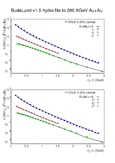
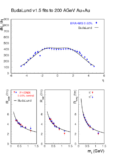
Figure 1: Solid line shows the simultaneous Buda-Lund v1.5 fit to final Au+Au data at $\sqrt{s_{\mbox{\tiny\rm NN}}}=200$ GeV. The transverse mass distributions of identified particles are measured by PHENIX [17] the pseudorapidity distributions of charged particles are measured by BRAHMS [18], the transverse mass dependence of the radius parameters are data of PHENIX [19]. Note that the identified particle spectra are published in more detailed centrality classes, but we recombined the 0-30% most central collisions so that the fitted spectra and radii be obtained in the same centrality class.

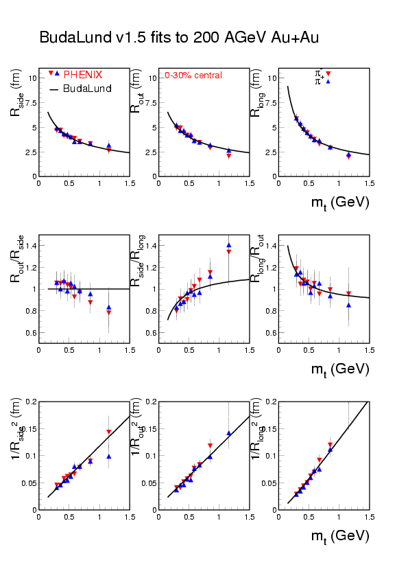
Figure 2: Top row shows the transverse mass dependence of the side, out and longitudinal HBT radii, the central line shows their pairwise ratio (usually only $R_{\mbox{\rm out}}/R_{\mbox{\rm side}}$ is shown) together with the Buda-Lund fits, vers. 1.5. The bottom line shows the inverse of the squared radii. The intercept of the curves in this row is within errors zero for the two transverse components, so the fugacity is within errors independent of the transverse coordinates. However, the intercept is nonzero in the longitudinal direction, which makes the fugacity (hence particle ratios) rapidity dependent. See also ref. [1] for a similar plot at $\sqrt{s_{\mbox{\tiny\rm NN}}}=130$ GeV.

Let us clarify first the meaning of the parameters shown in Table 1. The temperature at the center of the fireball at the mean freeze-out time is denoted by $T_{0}\equiv T(r_{x}=r_{y}=0,\tau=\tau_{0})$. The surface temperature is also a characteristic, kind of an average temperature, and its value is always $T_{s}\equiv T(r_{x}=r_{y}=R_{s},\tau=\tau_{0})=T_{0}/2$. In fact this relationship defines the “surface” radius $R_{s}$. During the particle emission, the system may cool due to evaporation and expansion, this is measured by the “post-evaporation temperature” $T_{e}\equiv T(r_{x}=r_{y}=0,\tau=\tau_{0}+\sqrt{2}\Delta\tau)$. In the presented cases, the strength of the transverse flow is measured by $\langle u_{t}^{\prime}\rangle$, its value at the “surface radius” $R_{s}$. The “mean freeze-out time” parameter is denoted by $\tau_{0}$ and the “duration” of particle emission, or the width of the freeze-out time distribution is measured by $\Delta\tau$. The fugacity distribution varies on the characteristic transverse scale given by the “geometrical radius” $R_{G}$. Finally, the width of the space-time rapidity distribution, or the longitudinal variation scale of the fugacity distribution is measured by the parameter $\Delta\eta$.

Perhaps it could be more appropriate to directly fit the transverse Hubble constant, $H_{t}=\langle u_{t}^{\prime}\rangle/R_{s}$ to the data, as this value is not sensitive to the length-scale chosen to evaluate the “average” transverse flow $\langle u_{t}^{\prime}\rangle$. In the case of parameters shown in Table 1, the density drop in the transverse direction is dominated by the cooling of the local temperature distribution in the transverse direction, and not so much by the change of the fugacity distribution. That is why we fitted here $\langle u_{t}^{\prime}\rangle$ at the “surface radius” $R_{s}$. Note also that $\tau_{0}$ could more properly be interpreted as the inverse of the longitudinal Hubble constant $H_{l}$, which is only an order of magnitude estimate of the mean freeze-out time, similarly to how the inverse of the present value of the Hubble constant in astrophysics provides only an order of magnitude estimate of the life-time of our Universe. The feasibility of directly fitting the transverse and longitudinal Hubble constants to data will be investigated in a subsequent publication.

Let us also note, that we have fitted the absolute normalized spectra for identified particles, and the normalization conditions were given by central chemical potentials $\mu_{0}$ that were taken as free normalization parameters for each particle species. All these directly fitted parameters are made public at [20]. From these values, we have determined the net bariochemical potential as $\mu_{B}=\mu_{p}-\mu_{\overline{p}}$. Although this parameter is not directly fitted but calculated, we have included $\mu_{B}$ in Table 1, so that our results could be compared with other successful models of two-particle Bose-Einstein correlations at RHIC, namely the AMPT cascade [26], Tom Humanic’s cascade [27], the blast-wave model [28, 29], the Hirano-Tsuda numerical hydro [30] and the Cracow “single freeze-out thermal model”  [31, 32, 33].

Now, we are ready for the discussion of the results in Table 1. In case of more central collisions at the lower RHIC energies, a well defined minimum was found, with accurate error matrix and a statistically acceptable fit quality, $\chi^{2}$/NDF= 158/180, that corresponds to a confidence level of 88 %. (These fit results were shown graphically on Figs. 1 and 2 of ref. [1], and the parameters are summarized in the second column of Table 1.) In the case of the less central but more energetic Au+Au collisions, the obtained $\chi^{2}/\mbox{\rm NDF}$ fit is too small. Note that in these fits we added the systematic and statistical errors in quadrature, and this procedure is preliminary and has to be revisited before we can report on the final values of the fit parameters and determine their error bars. It could also be advantageous to analyze a more central data sample, or the centrality dependence of the radius parameters and the pseudorapidity distributions, or to fit additional data of STAR and PHOBOS too, so that the parameters of the Buda-Lund hydro model could be determined with smaller error bars.

At present, we find that $T_{0}>T_{c}=172\pm 3$ MeV [3] by 3 $\sigma$ in case of the 0-30 % most central Au+Au data at $\sqrt{s_{\mbox{\tiny\rm NN}}}=200$ GeV, while $T_{0}>T_{c}$ by more than 5 $\sigma$ in case of the 0-5(6) % most central Au+Au data at $\sqrt{s_{\mbox{\tiny\rm NN}}}=130$ GeV. Thus this signal of a cross-over transition to quark deconfinement is not yet significant in the more energetic but less central Au+Au data sample, while it is significant at the more central, but less energetic sample. In this latter case of 130 GeV Au+Au data, $R_{G}$ obviously became an irrelevant parameter, with $1/R_{G}\approx 0.$ . This is explicitly visible in Fig. 2 of ref. [1], where the last row indicates that the correlation radii are in the scaling limit and the fugacity distribution, $\exp\left[\mu(x)/T(x)\right]$ is independent of the transverse coordinates.

The Buda-Lund model predicted, see eqs. (53-58) in ref. [4] and also eqs. (26-28) in [12], that the linearity of the inverse radii as a function of $m_{t}$ can be connected to the Hubble flow and the temperature gradients. The slopes are the same for side, out and longitudinal radii if the Hubble flow (and the temperature inhomogeneities) become direction independent. The intercepts of the linearly extrapolated $m_{t}$ dependent inverse squared radii at $m_{t}=0$ determine $1/R_{G}^{2}$, or the magnitude of corrections from the finite geometrical source sizes, that stem from the $\exp[\mu(x)/T(x)]$ terms. We can see on Fig. 2, that these corrections within errors vanish also in $\sqrt{s_{\mbox{\tiny\rm NN}}}=200$ Au+Au collisions at RHIC. This result is important, because it explains, why thermal and statistical models are successful at RHIC: if $\exp[\mu(x)/T(x)]=\exp(\mu_{0}/T_{0})$, then this factor becomes an overall normalization factor, proportional to the particle abundances. Indeed, we found that when the finite size in the transverse direction is generated by the $T(x)$ distribution, the quality of the fit increased and we had no degenerate parameters in the fit any more. This is also the reason, why we interpret $R_{s}$, given by the condition that $T(r_{x}=r_{y}=R_{s})=T_{0}/2$, as a “surface” radius: this is the scale where particle density drops.

Note that we have obtained similarly good description of these data if we require that the four-velocity field is a fully developed, three-dimensional Hubble flow, with $u^{\nu}=x^{\nu}/\tau$, however, we cannot elaborate on this point here due to the space limitations [2].

4 Conclusions

Table 1, Figures 1 and 2 indicate that the Buda-Lund hydro model works well both at the lower and the higher RHIC energies, and gives a good quality description of the transverse mass dependence of the HBT radii. For the dynamical reason, see refs. [12] and [4]. In fact, even the time evolution of the entrophy density can be solved from the fit results, $s(\tau)=s_{0}(\tau_{0}/\tau)^{3}$, which is the consequence of the Hubble flow, $u^{\nu}=x^{\nu}/\tau$, a well known solution of relativistic hydrodynamics, see also ref. [9]. This is can be considered as the resolution of the RHIC HBT “puzzle”, although a careful search of the literature indicates that this “puzzle” was only present in models that were not tuned to CERN SPS data [34].

We also observe that the central temperature is $T_{0}=214\pm 7$ MeV in the most central Au+Au collisions at $\sqrt{s_{\mbox{\tiny\rm NN}}}=130$ GeV, and we find here a net bariochemical potential of $\mu_{B}=77\pm 38$ MeV. Recent lattice QCD results indicate [3], that the critical temperature is within errors a constant of $T_{c}=172\pm 3$ MeV in the $0\leq\mu_{B}\leq 300$ MeV interval. Our results clearly indicate $(T,\mu_{B})$ values above this critical line, which is a significant, more than 5 $\sigma$ effect. The present level of precision and the currently fitted PHENIX and BRAHMS data set does not yet allow a firm conclusion about such an effect at $\sqrt{s_{\mbox{\tiny\rm NN}}}=200$ GeV, however, a similar behavior is seen on a 3 standard deviation level. This can be interpreted as a hint at quark deconfinement at $\sqrt{s_{\mbox{\tiny\rm NN}}}=200$ GeV at RHIC.

Finding similar parameters from the analysis of the pseudorapidity dependence of the elliptic flow, it was estimated in ref. [2] that 1/8th of the total volume is above the critical temperature in Au+Au collisions at $\sqrt{s_{\mbox{\tiny\rm NN}}}=130$ GeV, at the time when pions are emitted from the source. We interpret this result as an indication for quark deconfinement and a cross-over transition in Au+Au collisions at $\sqrt{s_{\mbox{\tiny\rm NN}}}=130$ GeV at RHIC. This result was signaled first in ref. [34] in a Buda-Lund analysis of the final PHENIX and STAR data on midrapidity spectra and Bose-Einstein correlations, but only at a three standard deviation level. By including the pseudorapidity distributions of BRAHMS and PHOBOS, the $T_{0}\gg T_{c}$ effect became significant in most central Au+Au collisions at $\sqrt{s_{\mbox{\tiny\rm NN}}}=130$ GeV. We are looking forward to observe, what happens with the present signal in Au+Au collisions at $\sqrt{s_{\mbox{\tiny\rm NN}}}=200$ GeV, if we include STAR and PHOBOS data to the fitted sample.

The above observation of temperatures, that are higher than the critical one, is only an indication, with other words, an indirect proof for the production of a new phase, as the critical temperature is not extracted directly from the data, but taken from recent lattice QCD calculations.

More data are needed to clarify the picture of quark deconfinement at the maximal RHIC energies, for example the centrality dependence of the Bose-Einstein (HBT) radius parameters could provide very important insights.

References

- [1] M. Csanád, T. Csörgő, B. Lörstad, A. Ster, Act. Phys. Pol. B35, 191 (2004), nucl-th/0311102.
- [2] M. Csanád, T. Csörgő and B. Lörstad, nucl-th/0310040.
- [3] Z. Fodor and S. D. Katz, JHEP 0203 (2002) 014
- [4] T. Csörgő and B. Lörstad, Phys. Rev. C 54 (1996) 1390
- [5] T. Csörgő and B. Lörstad, Nucl. Phys. A 590 (1995) 465C
- [6] T. Csörgő, Heavy Ion Phys. 15 (2002) 1, hep-ph/0001233.
- [7] T. Csörgő, B. Lörstad and J. Zimányi, Z. Phys. C 71 (1996) 491
- [8] T. Csörgő, F. Grassi, Y. Hama, T. Kodama, Phys. Lett. B565, 107 (2003)
- [9] T. Csörgő, L. Csernai, Y. Hama, T. Kodama, nucl-th/0306004.
- [10] T. Csörgő, nucl-th/9809011.
- [11] T. Csörgő, hep-ph/0111139.
- [12] T. Csörgő and J. Zimányi, Heavy Ion Phys. 17, 281 (2003), nucl-th/0206051.
- [13] S. Chapman, P. Scotto and U. Heinz, Heavy Ion Phys. 1 (1995) 1, hep-ph/9409349.
- [14] A. Ster, T. Csörgő and J. Beier, Heavy Ion Phys. 10 (1999) 85, hep-ph/9810341.
- [15] T. S. Biró, Phys. Lett. B 474 (2000) 21
- [16] T. S. Biró, Phys. Lett. B 487 (2000) 133
- [17] S. S. Adler et al. [PHENIX Collaboration], [arXiv:nucl-ex/0307022].
- [18] I. G. Bearden et al. [BRAHMS Collaboration], Phys. Rev. Lett. 88 (2002) 202301
- [19] S. S. Adler [PHENIX Collaboration], arXiv:nucl-ex/0401003.
- [20] http://www.kfki.hu/csorgo/budalund/
- [21] I. G. Bearden et al. [BRAHMS Collaborations], Phys. Lett. B 523 (2001) 227
- [22] B. B. Back et al. [PHOBOS Collaboration], Phys. Rev. Lett. 87 (2001) 102303
- [23] K. Adcox et al. [PHENIX Collaboration], Phys. Rev. Lett. 88 (2002) 242301
- [24] K. Adcox et al. [PHENIX Collaboration], Phys. Rev. Lett. 88 (2002) 192302
- [25] C. Adler et al. [STAR Collaboration], Phys. Rev. Lett. 87 (2001) 082301
- [26] Z. W. Lin, C. M. Ko and S. Pal, Phys. Rev. Lett. 89 (2002) 152301,
- [27] T. J. Humanic, Nucl. Phys. A 715 (2003) 641
- [28] F. Retiere, J. Phys. G 30 (2004) S335
- [29] F. Retiere and M. A. Lisa, arXiv:nucl-th/0312024.
- [30] T. Hirano and K. Tsuda, Nucl. Phys. A 715 (2003) 821
- [31] W. Broniowski, A. Baran and W. Florkowski, AIP Conf. Proc. 660 (2003) 185
- [32] W. Florkowski and W. Broniowski, AIP Conf. Proc. 660 (2003) 177
- [33] W. Broniowski and W. Florkowski, Phys. Rev. Lett. 87 (2001) 272302
- [34] T. Csörgő and A. Ster, Heavy Ion Phys. 17 (2003) 295, nucl-th/0207016.