Self-consistent Green’s function method
for nuclei and nuclear matter

Abstract

Recent results obtained by applying the method of self-consistent Green’s functions to nuclei and nuclear matter are reviewed. Particular attention is given to the description of experimental data obtained from the (e,e^′p) and (e,e^′2N) reactions that determine one and two-nucleon removal probabilities in nuclei since the corresponding amplitudes are directly related to the imaginary parts of the single-particle and two-particle propagators. For this reason and the fact that these amplitudes can now be calculated with the inclusion of all the relevant physical processes, it is useful to explore the efficacy of the method of self-consistent Green’s functions in describing these experimental data. Results for both finite nuclei and nuclear matter are discussed with particular emphasis on clarifying the role of short-range correlations in determining various experimental quantities. The important role of long-range correlations in determining the structure of low-energy correlations is also documented. For a complete understanding of nuclear phenomena it is therefore essential to include both types of physical correlations. We demonstrate that recent experimental results for these reactions combined with the reported theoretical calculations yield a very clear understanding of the properties of all protons in the nucleus. We propose that this knowledge of the properties of constituent fermions in a correlated many-body system is a unique feature of nuclear physics.

TRIUMF preprint: TRI-PP-03-40

1 Introduction

Various approaches exist to deal with the nuclear many-body problem. A comparison of these approaches has recently been given in Ref. [2]. In this review only one specific method is singled out for discussion. This method is most intimately connected to quantum field theory since it corresponds to the nonrelativistic implementation of this approach to the many-body problem. While the propagator or Green’s function method was the most important tool in the formal development of many-body theory [3] - [7], only in the last ten years has it been applied to many-body problems beyond its mean-field implementation (the Hartree-Fock approximation). Examples of such applications have appeared in atomic [8] and condensed matter physics [9]. In the atomic case, the essential new development involves taking the self-consistent determination of the electron propagator from the Hartree-Fock level to the fully self-consistent inclusion of the second-order self-energy. Important quantitative improvements over the Hartree-Fock results are obtained for standard quantities like the binding energy but other experimental data like spectroscopic factors are significantly improved as well [8]. In the case of the electron gas, the self-consistent determination of the electron propagator involves the summation of all ring diagrams in the self-energy which is necessary to treat the well known divergence of the Coulomb interaction in an infinite system. Also in this case, one obtains a much improved description of the energy per particle [9] essentially in agreement with the benchmark Monte Carlo results of Ref. [10].

In the nuclear case, similar developments have taken place which have focused on the self-consistent treatment of short-range correlations (SRC) in nuclear matter by including ladder diagrams in the self-energy. For finite nuclei, the self-consistent treatment of long-range correlations (LRC) has been considered at different levels of sophistication. The nuclear case is particularly unique due to the availability of a magnificent set of experimental data which have illuminated in great detail the properties of the nucleon propagator in the medium. These experiments involve nucleon knockout reactions induced by electrons which are measured in coincidence with the ejected proton [11] - [17]. These experiments identify in an essentially unambiguous manner the removal probability of protons near the Fermi energy from a variety of target nuclei. The results of these experiments have clearly identified the need to consider nucleon properties beyond the mean-field since these removal probabilities have consistently been about 35% below the simple shell-model value of 1 for closed-shell systems. By identifying these removal probabilities experimentally, one gains crucial insight into those quantities which determine the proton propagator in the medium. It is then natural to approach the theoretical description of these data by employing the propagator method.

It is the purpose of this review to document the recent development of the theoretical understanding of these (e,e^′p) data over the last ten years. The wonderful interplay between experimental and theoretical work will be exploited and presented in some detail. The currently emerging picture suggests that the properties of all protons in the nucleus are within the domain of experimental scrutiny including those with high momenta. The accompanying improved theoretical understanding of these properties of protons in the nucleus has also acted as a catalyst for the renewed study of the nuclear-matter saturation problem.

The paper starts in Sec. 2 with the introduction of the relevant formalism for the determination of the one and two-particle propagators. By employing the equation of motion formulation it becomes straightforward to introduce the concept of self-consistency necessary for a proper description of the dynamics as it is encountered in nuclei and nuclear matter. Sec. 3 is devoted to a brief pedagogical exploration of the relation between the experimental data accessible in (e,e^′p) and (e,e^′2N) reactions and the relevant theoretical quantities introduced in Sec. 2. A detailed analysis of Green’s function calculations for nuclear matter is presented in Sec. 4. We limit the discussion to zero-temperature results and do not cover neutron matter. This section starts with a brief introduction of the material and gives a short review of the first-generation results for spectral functions to establish a framework for the assessment of the most recent fully self-consistent results. These early calculations solved the scattering problem in the medium by propagating mean-field (mf) nucleons in the medium which is equivalent to the so-called Galitski-Feynman treatment [18]. A similar approach is adopted to generate spectral functions for $\Lambda$ hyperons which are compared to the corresponding results for nucleons. Particular attention is given to recent developments involving the fully self-consistent inclusion of SRC. The results for this second generation of spectral functions are discussed together with an analysis of the scattering process in the medium that underlies the properties of individual nucleons in nuclear matter. A detailed discussion of healing properties of nucleons in the medium is presented in order to resolve the paradox that arises when the original discussion of healing [19, 20] is confronted with recent (e,e^′p) data. The consequences for the nuclear matter saturation properties including these recent developments concludes this section.

Section 5 is devoted to a discussion of the results for the single-particle (sp) propagator in finite nuclei. After a brief introduction we start this section with an overview of the early calculations for the spectral strength distribution. The influence of LRC is illustrated by a direct comparison of the spectral strength distribution with the data. The dual role of SRC in determining the distribution of the sp strength is then clarified in detail. The important influence of both low-energy particle-particle (pp), hole-hole (hh), and particle-hole (ph) correlations in the form of collective behavior in determining the low-energy sp properties is emphasized to provide the basis of a new development involving the Faddeev technique applied to the many-body problem. This new technique is then reviewed and shown to incorporate the correct way to include these correlations simultaneously. State of the art results for ${}^{16}\textrm{O}$ demonstrate that further improvement of the description of LRC is required for a complete description of the experimental data. This is further illustrated by analyzing the collective phonons in ${}^{16}\textrm{O}$ that form the ingredients of the Faddeev summation. A comparison with the experimental excitation spectrum of ${}^{16}\textrm{O}$ demonstrates that further improvement of the theoretical description of this spectrum is necessary. A first step in this direction is presented which takes the self-consistent coupling of single phonons to two phonons into account.

A discussion of recent calculations of two-proton removal cross sections follows including a comparison with experimental data. Recent experimental developments will be briefly highlighted which elucidate the properties of all protons in the domain of the traditional nuclear mean-field. These results are also discussed in Sec. 5 together with recent attempts to determine the properties of high-momentum protons in the nucleus. In Sec. 6 the results are summarized in as far as they clarify the properties of protons in the nucleus. A brief comparison with other correlated many-body systems is also presented there. A final summary and outlook for future work is given in Sec. 7.

2 Formal development

2.1 Single-particle Green’s function

The nuclear systems to be discussed in this review will be described as a collection of nonrelativistic nucleons interacting by means of a two-body interaction $\hat{V}$ that describes nucleon-nucleon (NN) scattering data up to pion production threshold. One can generate a zero-order approximation of the system under study by introducing an appropriate mean-field potential $\hat{U}$ and splitting the Hamiltonian into an unperturbed one-body part $\hat{H}_{0}=\hat{T}+\hat{U}$ and a residual interaction $\hat{H}_{1}=\hat{V}-\hat{U}$. The total Hamiltonian can then be written as

$$\hat{H}~{}=~{}\hat{H}_{0}~{}+~{}\hat{H}_{1}~{}=~{}\sum_{\alpha}\varepsilon^{0}_{\alpha}~{}c^{{\dagger}}_{\alpha}c_{\alpha}~{}+~{}\left({\textstyle\frac{1}{4}}\sum_{\alpha\beta\gamma\delta}V_{\alpha\beta,\gamma\delta}~{}c^{{\dagger}}_{\alpha}~{}c^{{\dagger}}_{\beta}~{}c_{\delta}~{}c_{\gamma}~{}-~{}\sum_{\alpha\beta}U_{\alpha,\beta}~{}c^{{\dagger}}_{\alpha}c_{\beta}\right)\;,$$ (1)

where we have chosen to use a set of sp states $\{\alpha\}$ that diagonalize $H_{0}$ with eigenvalues $\{\varepsilon^{0}_{\alpha}\}$, $c^{{\dagger}}_{\alpha}$ ($c_{\alpha}$) are the creation (destruction) operators of a particle in the state $\alpha$, $V_{\alpha\beta,\gamma\delta}$ the antisymmetrized matrix elements of $\hat{V}$, and $U_{\alpha,\beta}$ correspond to the matrix elements of $\hat{U}$. In general, the best choice of $\hat{H}_{0}$ (and therefore of the basis $\{\alpha\}$) depends on the symmetry properties of the system under study. For infinite nuclear matter translational invariance suggests the use of momentum eigenstates without any need for choosing an auxiliary potential, while for finite nuclei one needs to employ a potential (e.g. of the harmonic oscillator or Woods-Saxon type) to localize the nucleons. Obviously, the spectrum $\{\varepsilon^{0}_{\alpha}\}$ can contain both discrete and/or continuum states and we therefore use the summation symbols in Eq. (1) to include both a summation over the discrete part of the spectrum as well as an integration over the continuum part. This convention will be used throughout this section.

Three-body forces are known to produce important effects on details of nuclear spectra [21, 22]. These forces can in principle be added to Eq. (1) and included in the formalism. Since the calculations to be discussed in this paper do not explicitly include their effects, we will therefore not consider them in the following but we will discuss some related issues in Sec. 4.7.

The experimental information concerning sp properties of a many-body nuclear system is usually obtained by probing the ground state $|\Psi^{A}_{0}\rangle$ of a nucleus with $A$ particles by the addition or removal of a nucleon as discussed in more detail in Sec. 3. The one-body (sp) propagator (or two-point Green’s function) associated with the state $|\Psi^{A}_{0}\rangle$ embodies this information and is defined according to [3] - [7]

$$g_{\alpha\beta}(t-t^{\prime})~{}=~{}-i~{}\langle\Psi^{A}_{0}|~{}\mathcal{T}[c_{\alpha}(t)c^{{\dagger}}_{\beta}(t^{\prime})]~{}|\Psi^{A}_{0}\rangle\;,$$ (2)

where $\mathcal{T}[...]$ represents the time-ordering operation and $c^{{\dagger}}_{\alpha}(t)$ and $c_{\alpha}(t)$ now correspond to operators in the Heisenberg picture (with $\hbar=1$). For $\tau=t-t^{\prime}>0$, Eq. (2) incorporates the probability amplitude for adding a particle in a state $\beta$ and removing it from a state $\alpha$ after a time $\tau$. Similarly, a hole can be generated in $\alpha$ and annihilated from $\beta$ after a time $t^{\prime}-t>0$.

The information contained in the sp propagator $g_{\alpha\beta}(\tau)$ becomes more transparent after Fourier transformation from the time to the energy formulation. After separating the positive and negative time contributions in Eq. (2) one includes the completeness relations for $A\pm 1$ nucleons to obtain

$$g_{\alpha\beta}(\omega)~{} = ~{}\frac{1}{2\pi}\int_{-\infty}^{+\infty}d\tau~{}e^{-i\omega\tau}g_{\alpha\beta}(\tau)$$ (3)

$$= ~{}\sum_{n}\frac{\langle\Psi^{A}_{0}|c_{\alpha}|\Psi^{A+1}_{n}\rangle\langle\Psi^{A+1}_{n}|c^{{\dagger}}_{\beta}|\Psi^{A}_{0}\rangle}{\omega-\varepsilon^{+}_{n}+i\eta}~{}+~{}\sum_{k}\frac{\langle{\Psi^{A-1}_{k}}|c_{\alpha}|{\Psi^{A}_{0}}\rangle\langle{\Psi^{A}_{0}}|c^{{\dagger}}_{\beta}|{\Psi^{A-1}_{k}}\rangle}{\omega-\varepsilon^{-}_{k}-i\eta}\;,$$

which is know as the Lehmann representation of the sp propagator [23]. Here, and in the following, the indices $n$ and $k$ enumerate the eigenstates of the system with $A+1$ and $A-1$ particles, respectively. As discussed above, the summations are intended to represent sums over the discrete spectrum and integrals over the continuum part. The poles $\varepsilon^{+}_{n}\equiv E^{A+1}_{n}-E^{A}_{0}$ and $\varepsilon^{-}_{k}\equiv E^{A}_{0}-E^{A-1}_{k}$ in Eq. (3) correspond to the excitation energies of the $A\pm 1$-body systems with respect to the ground-state energy $E^{A}_{0}$. Equation (3) includes information on the transition amplitudes for the addition and removal of a nucleon in the numerator and these excitation energies in the denominator. This feature illustrates the wealth of information in the sp propagator that can be compared to experimental data. Experimentally, this information is typically obtained in the form of the one-hole spectral function which is related to the imaginary part of $g(\omega)$ by

$$S^{h}_{\alpha}(\omega) = \frac{1}{\pi}~{}{\rm Im}\;g_{\alpha\alpha}(\omega)$$ (4)

$$= \sum_{k}\left|\langle{\Psi^{A-1}_{k}}|c_{\alpha}|{\Psi^{A}_{0}}\rangle\right|^{2}\delta(\omega-\varepsilon^{-}_{k})~{}~{}~{}~{}~{}~{}~{}~{}~{}\omega<\varepsilon^{-}_{F}\;,$$

for nucleon removal. The corresponding particle spectral function is given by

$$S^{p}_{\alpha}(\omega) = -\frac{1}{\pi}~{}{\rm Im}\;g_{\alpha\alpha}(\omega)$$ (5)

$$= \sum_{n}\left|\langle{\Psi^{A+1}_{n}}|c^{{\dagger}}_{\alpha}|{\Psi^{A}_{0}}\rangle\right|^{2}\delta(\omega-\varepsilon^{+}_{n})~{}~{}~{}~{}~{}~{}~{}~{}~{}\omega>\varepsilon^{+}_{F}\;,$$

and in this form is mostly of theoretical relevance. $S^{h}(\omega)$ ( $S^{p}(\omega)$ ) represent the probability for removing (adding) a particle from (to) an (in) orbital $\alpha$ while leaving the residual system in a state with energy $-\omega$ ($\omega$) relative to the ground state $E^{A}_{0}$ of the system with $A$ particles. The Fermi energies $\varepsilon_{F}^{+}$ and $\varepsilon_{F}^{-}$ denote the minimum excitation energy needed to remove or add a particle and are given by

$$\varepsilon^{-}_{F} \equiv E^{A}_{0}-E^{A-1}_{0}\;$$ (6a)

$$\varepsilon^{+}_{F} \equiv E^{A+1}_{0}-E^{A}_{0}\;.$$ (6b)

For infinite systems with a ground state that does not exhibit pairing these quantities are equal in the thermodynamic limit and will be referred to as the Fermi energy $\varepsilon_{F}=\varepsilon_{F}^{+}=\varepsilon_{F}^{-}$. In finite nuclei a considerable difference exists between $\varepsilon_{F}^{+}$ and $\varepsilon_{F}^{-}$ for the closed-shell nuclei considered in this review.

An important experimental result, when considering the knockout of nucleons from a mf orbit, is the reduction of the observed cross section with respect to the prediction of the independent-particle model (IPM) [12] - [17] as discussed in Sec. 3. This is due to the fact that these orbits are only partially occupied in the correlated system. From the theoretical point of view, this effect can be quantified by looking at the normalization of the overlap integral between the initial and the final states, $\langle\Psi^{A-1}_{k}|c_{\alpha}|\Psi^{A}_{0}\rangle$ [17] (see Sec. 3 for more details). Considering the transition to a state $k$ of the $A-1$ particle system one may define the theoretical spectroscopic factor as

$$S_{k}=\sum_{\alpha}\left|\langle{\Psi^{A-1}_{k}}|c_{\alpha}|{\Psi^{A}_{0}}\rangle\right|^{2}\;.$$ (7)

Obviously, this quantity is also contained in the hole spectral function given in Eq. (4).

The information on nuclear structure that is contained in Eqs. (4) and (5) can be fruitfully compared to the case of an uncorrelated mf system. When the residual interaction is neglected in Eq. (1), the wave function of the system is an eigenstate of the unperturbed Hamiltonian $\hat{H}_{0}$. The corresponding ground state, $|\Phi^{A}_{0}\rangle$, is a Slater determinant with all the lowest sp orbitals fully occupied up to the hole Fermi energy $\varepsilon_{F}^{-}$, while those above are empty. The unperturbed propagator associated with $|\Phi^{A}_{0}\rangle$ is given by

$$g^{(0)}_{\alpha\beta}(\omega)~{}=~{}\delta_{\alpha,\beta}\left\{\frac{\theta(\alpha-F)}{\omega-\varepsilon^{0}_{\alpha}+i\eta}~{}+~{}\frac{\theta(F-\alpha)}{\omega-\varepsilon^{0}_{\alpha}-i\eta}\right\}\;,$$ (8)

where $\theta(\alpha-F)$ ( $\theta(F-\alpha)$ ) is equal to 0 (1) if $\alpha$ is an occupied state and it is 1 (0) otherwise. The poles of $g^{(0)}(\omega)$ correspond to the unperturbed sp energies and the forward and backward going contributions contain either orbitals that are outside or inside the Fermi sea $F$, respectively. We note that in order to consider the whole sp spectrum, one needs to consider both the particle and hole states. The hole spectroscopic factors associated with Eq. (8) are exactly one for those states that belong to the Fermi sea and zero otherwise, reflecting the occupancy of the orbitals in $|\Phi^{A}_{0}\rangle$. A deviation from unity occurs in a finite system when the center-of-mass motion is properly treated [24].

This simple mf picture is modified when one includes many-body correlations, generated by the term $\hat{H}_{1}$ in the full Hamiltonian. Comparing Eqs. (3) and (8), one can still find a correspondence between the unperturbed energies of particle orbitals and the excitation spectrum $\{n\}$ of the system with $A+1$ nucleons and between the hole energies and the spectrum $\{k\}$ of $A-1$ nucleons. However, a larger number of states can appear in the correlated systems due to the mixing of sp excitations with more complicated configurations. As discussed in Sec. 2.2, these more complicated states are at least of two-particle$-$one-hole (2p1h) or two-hole$-$one-particle (2h1p) character. In the case of nuclear systems, the mixing of these states is generated by the presence of both collective modes of the system and the relevance of short-range effects associated with the nature of the underlying two-body interaction $\hat{V}$. This mixing generates a large number of sp fragments (or poles in Eq.(3) ). At the same time, it reduces the total sp strength of each peak of the IPM and redistributes it among all the fragments of both particle and hole type, over a wide range of energies. The reduction of the spectroscopic factors (7) from 1 can therefore be taken as a direct measure of correlations in the system.

The occupation number of a given sp particle state in the correlated ground state can be obtained from the hole spectral function

$$n_{\alpha}=\langle{\Psi^{A}_{0}}|c^{\dagger}_{\alpha}c_{\alpha}|{\Psi^{A}_{0}}\rangle=\sum_{k}\left|\langle{\Psi^{A-1}_{k}}|c_{\alpha}|{\Psi^{A}_{0}}\rangle\right|^{2}=\int_{-\infty}^{\varepsilon^{-}_{F}}\!\!\!d\omega\;S^{h}_{\alpha}(\omega)\;\;,$$ (9)

where the integral ranges over all the fragments of the orbital $\alpha$ that are spread over different quasihole energies, as discussed above. Correlations have the effect of reducing the occupation of the orbitals in the Fermi sea (which would be 1 for the unperturbed state $|\Phi^{A}_{0}\rangle$) and to partially populate states that were originally empty. A measure of the emptiness of the orbital is obtained by integrating the particle spectral function

$$d_{\alpha}=\langle{\Psi^{A}_{0}}|c_{\alpha}c^{\dagger}_{\alpha}|{\Psi^{A}_{0}}\rangle=\sum_{n}\left|\langle{\Psi^{A+1}_{n}}|c^{\dagger}_{\alpha}|{\Psi^{A}_{0}}\rangle\right|^{2}=\int^{+\infty}_{\varepsilon^{+}_{F}}\!\!\!d\omega\;S^{p}_{\alpha}(\omega)\;\;.$$ (10)

Using the fermion anticommutation relations, one obtains the sum rule $n_{\alpha}+d_{\alpha}=1$, valid for any orbital $\alpha$. This is an important result since it connects information on the removal and the addition of a particle to the system which refer to quite different experimental processes. It also supports the suggestion that both quasiparticle and quasihole states, together, form a natural space in which to study sp properties [25].

It is also worth noting that the knowledge of the sp propagator allows the evaluation of the expectation value of any one-body operator $\hat{O}$ according to

$$\langle\Psi^{A}_{0}|~{}\hat{O}~{}|\Psi^{A}_{0}\rangle=\sum_{\alpha\;\beta}O_{\alpha,\beta}\int\frac{d\omega}{2\pi i}e^{i\omega\eta}g_{\beta\alpha}(\omega)\;.$$ (11)

Moreover, it is also possible to compute the energy of the ground state by means of the Midgal-Galitski-Koltun (MGK) sum rule [26, 27]

$$E^{A}_{0}=\langle{\Psi^{A}_{0}}|\hat{H}|{\Psi^{A}_{0}}\rangle=\frac{1}{2}\int_{-\infty}^{\varepsilon^{-}_{F}}d\omega\;\sum_{\alpha\beta}\left(\langle\alpha|\hat{T}|\beta\rangle~{}+~{}\omega\;\delta_{\alpha\beta}\right)\frac{1}{\pi}{\rm Im}\;g_{\beta\alpha}(\omega)\;\;,$$ (12)

which is an exact result when only two-body forces are considered. Equation (12) is noteworthy since it includes the expectation value of the potential energy, which is a two-body quantity, solely in terms of the one-body propagator. This contribution is obtained by integrating over all possible separation energies the product of this separation energy multiplied by the corresponding spectral strength (summed over all relevant sp orbits). This result is very important because it shows how the details of the hole spectral distribution strongly influence the binding energy of the correlated ground state. The occupation number $n_{\alpha}$ yields information about the overall population of the state $\alpha$ but the energy integral in Eq. (9) loses track of the energies at which these nucleons are located inside the nucleus. In the case of nuclear systems a sizable amount of strength is shifted down to very negative sp energies by short-range and tensor correlations, with important consequences for the binding energy of the system as discussed in Sec. 4.7.

2.2 Equation of motion method and Dyson equation

The Green’s function (2) can be computed by applying the methods of quantum field theory. This path was developed in the fifties by Migdal and Galitski [26, 18] and by Martin and Schwinger [5] and makes use of a Feynman-diagram expansion. The method has found extensive application in several areas of many-body physics including atomic, condensed matter, and nuclear physics. One possible approach consists in choosing the propagator $g^{(0)}(\omega)$ as a starting point and to generate a perturbative expansion in the interaction $\hat{H}_{1}$. The diagram rules for calculating the contributions to $g(\omega)$ can be found in several text books (see for example Refs. [3, 4, 7]). In general, the expansion will contain diagrams that describe all the possible ways in which the unperturbed sp propagator interacts with particle and hole excitations inside the system. Due to the strongly repulsive character of the nuclear force a truncation of the perturbative expansion to a given power in the interaction $\hat{H}_{1}$ is quite inadequate and it becomes necessary to include the relevant physical processes by means of all-order summation techniques. One therefore introduces the concept of the irreducible self-energy $\Sigma^{\star}(\omega)$ as the collection of all connected diagrams that are one-particle irreducible, that is, they cannot be separated by cutting a single propagator line. The sum of these contributions represents the effective interaction that a particle is subjected to when interacting with the nuclear medium as will be shown explicitly in Sec. 3. These contributions can be summed to all orders by the Dyson equation shown in Fig. 1 which generates the whole perturbation series as shown in Fig. 2. This Dyson equation is given by

$$g_{\alpha\beta}(\omega)~{}=~{}g^{(0)}_{\alpha\beta}(\omega)~{}+~{}\sum_{\gamma,\delta}g^{(0)}_{\alpha\gamma}(\omega)\;\Sigma^{\star}_{\gamma\delta}(\omega)\;g_{\delta\beta}(\omega)\;.$$ (13)

Figure 1: Graphical representation of the Dyson equation (Eq. (13) ). The double line represents the exact (dressed) sp propagator $g(\omega)$, while the single line stands for the unperturbed propagator $g^{(0)}(\omega)$.

Figure 2: Illustration of how the Dyson equation generates the expansion in which the irreducible self-energy $\Sigma^{\star}(\omega)$ is summed to all orders.

An alternatve derivation of Eq. (13) can be obtained by either considering the equation of motion for $g(\omega)$ [5] or working directly with the effective action functional [28]. The result is an exact formulation relating each many-body Green’s function to the exact propagators of higher order. This generates a hierarchy of relations between the two-, three- and $A$-body Green’s functions, of which Eq. (14) below is the first example [5, 6]. Employing the equation of motion for a Heisenberg operator $dc_{\alpha}(t)/dt=-i[c_{\alpha}(t),\hat{H}]$ one obtains the time derivative of Eq. (2) [3],

$$i\frac{\partial}{\partial t}g_{\alpha\beta}(t-t^{\prime})~{} = ~{}\delta(t-t^{\prime})\delta_{\alpha\beta}~{}+~{}\varepsilon^{0}_{\alpha}g_{\alpha\beta}(t-t^{\prime})~{}-~{}\sum_{\gamma}U_{\alpha\gamma}g_{\gamma\beta}(t-t^{\prime})$$ (14)

$$+ ~{}\frac{1}{2}\sum_{\eta,\gamma,\zeta}V_{\alpha\eta,\gamma\zeta}\;(-i)\;\langle\Psi^{A}_{0}|~{}T[c^{{\dagger}}_{\eta}(t)c_{\zeta}(t)c_{\gamma}(t)c^{{\dagger}}_{\beta}(t^{\prime})]~{}|\Psi^{A}_{0}\rangle\;.$$

This generates a term containing the 4-point Green’s function

$$g^{4-pt}_{\alpha\beta,\gamma\delta}(t_{1},t_{2};t_{3},t_{4})~{}=~{}-i~{}\langle\Psi^{A}_{0}|~{}T[c_{\beta}(t_{2})c_{\alpha}(t_{1})c^{{\dagger}}_{\gamma}(t_{3})c^{{\dagger}}_{\delta}(t_{4})]~{}|\Psi^{A}_{0}\rangle\;.$$ (15)

By contracting this with the matrix elements of the two-body interaction, as in the last term of Eq. (14), one can relate the expectation value of $\hat{V}$ to the one-body propagator (2), whence the MGK sum rule (12) follows.

In general, $g^{4-pt}$ can describe the propagation of either two-particle (pp), two-hole (hh) or particle-hole (ph) excitations depending of the ordering of its time arguments. From a diagrammatical point of view, this propagator is the sum of two contributions. The first is a diagram in which two different particles propagate, fully correlated, without any interaction among them. The second group defines the four-point vertex function $\Gamma^{4-pt}$ which includes all the diagrams in which two dressed particles can interact with each other, thereby generalizing the $T$ matrix for the scattering of two free particles. The corresponding contribution to $g^{4-pt}$ is simply obtained by adding external lines to this vertex. One therefore obtains

$$g^{4-pt}_{\alpha\beta,\gamma\delta}(t_{1},t_{2};t_{3},t_{4})~{} = ~{}i\left[g_{\alpha\gamma}(t_{1}-t_{3})\;g_{\beta\delta}(t_{2}-t_{4})~{}-~{}g_{\alpha\delta}(t_{1}-t_{4})\;g_{\beta\gamma}(t_{2}-t_{3})\right]$$ (16)

$$-~{}\int dt_{5}\int dt_{6}\int dt_{7}\int dt_{8}\sum_{\mu,\nu,\lambda,\eta}g_{\alpha\mu}(t_{1}-t_{5})g_{\beta\nu}(t_{2}-t_{6})$$

$$~{}~{}\times\;\Gamma^{4-pt}_{\mu\nu,\lambda\eta}(t_{5},t_{6};t_{7},t_{8})\;g_{\lambda\gamma}(t_{7}-t_{3})g_{\eta\delta}(t_{8}-t_{4})\;,$$

which is depicted in Fig. 3.

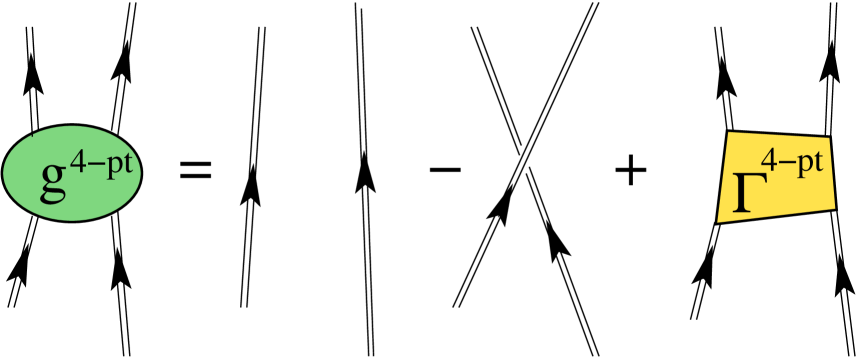
Figure 3: Diagrammatic structure of the four-point Green’s function in terms of the vertex function $\Gamma^{4-pt}$ (see Eq. (16) ).

The Dyson equation (13) can now be obtained by Fourier transformation of Eq.(14). Employing Eq. (8) one then finds an exact expression for the self-energy $\Sigma^{\star}(\omega)$ in terms of the sp propagator $g(\omega)$ and the vertex $\Gamma^{4-pt}$. By using Eq. (16) one obtains

$$\Sigma^{\star}_{\gamma\delta}(\omega)~{} = ~{}-~{}\langle\gamma|\hat{U}|\delta\rangle~{}+~{}\Sigma^{HF}_{\gamma\delta}$$ (17)

$$~{}-\frac{i^{2}}{2}\int\frac{d\omega_{1}}{2\pi}\int\frac{d\omega_{2}}{2\pi}\sum_{\mu,\nu,\lambda}\sum_{\alpha,\beta,\varepsilon}V_{\gamma\varepsilon,\alpha\beta}\;g_{\alpha\mu}(\omega_{1})g_{\beta\nu}(\omega_{2})$$

$$~{}~{}\times\Gamma^{4-pt}_{\mu\nu,\delta\lambda}(\omega_{1},\omega_{2};\omega,\omega_{1}+\omega_{2}-\omega)g_{\lambda\varepsilon}(\omega_{1}+\omega_{2}-\omega)$$

where the term $-\langle\gamma|\hat{U}|\delta\rangle$ subtracts the auxiliary potential which was added in the unperturbed Hamiltonian $\hat{H}_{0}$. This result is shown in part $a)$ of Fig. 4), The second term in Eq. (17) is the Hartree-Fock contribution to the self energy,

$$\Sigma^{HF}_{\alpha\beta}=\sum_{\gamma\delta}\int\frac{d\omega}{2\pi i}~{}e^{+i\omega\eta^{+}}~{}V_{\alpha\gamma,\beta\delta}~{}g_{\gamma\delta}(\omega)\;\;.$$ (18)

which represents the (energy-independent) interaction of the nucleon with the quasihole excitations inside the system. When all the higher-order terms of the self-energy are neglected, the solution of the Dyson equation $g(\omega)$ takes the same simple form as Eq. (8), which is equivalent to a Slater determinant description of the ground state. In this case the quasihole wave functions contained in $g(\omega)$ refer to completely filled orbitals and the iterative solution of Eqs. (13) and (18) generates the standard Hartree-Fock approximation.

Figure 4: Various possible expansions of the irreducible self-energy in terms of higher order many-body Green’s functions. In all cases the first two terms represent the mean-field contributions $-\hat{U}$ and the Hartree-Fock self-energy $\Sigma^{HF}$. The dynamic part of the self-energy can be expressed in terms of the four-point vertex function $\Gamma^{4-pt}$. Part $a)$ represents the relation given in Eq. (17), while the part $b)$ corresponds to an alternative derivation involving the time derivative of $g$ with respect to $t^{\prime}$. If $\Gamma^{4-pt}$ is approximated in such a way that the corresponding two diagrams in $a)$ and $b)$ are equivalent, the Dyson equation will satisfy appropriate sum rules. Part $c)$ gives the expansion in terms of the one-particle irreducible 2p1h/2h1p propagator $R(\omega)$, Eq (19). Note that the full four-time dependence of $\Gamma^{4-pt}$ is needed in principle, while in the $R(\omega)$ formulation one can specialize to a two-time quantity.

The many-body correlations beyond the nuclear mean field are included in the energy-dependent part of the self-energy. A possible expansion of this self-energy, in terms of $\Gamma^{4-pt}$, is given by the last term of Eq. (17) and shown diagrammatically in Fig. 4$a)$. One should note that Eq. (17) is formally exact and therefore the latter term contains implicitly the effect of both pp, hh, and ph collective excitations and their coupling to the sp motion. This is of course at the prize of having to keep track of the different time arguments in $\Gamma^{4-pt}$, which involves an awkward mathematical structure. When only the pp (hh) effects or the ph ones need to be studied, $\Gamma^{4-pt}$ can be conveniently approximated by the ladder or the ring series, respectively (to be described in Sec. 2.4). In these cases $\Gamma^{4-pt}$ reduces to a two-time quantity, i.e. depends on only one energy variable. In the cases where this simplification is not possible, Eq. (17) may no longer correspond to the best approach and it becomes useful to go one step further in the hierachy of Green’s functions by taking a second derivative in Eq. (14), with respect to the time argument $t^{\prime}$. This will result in introducing a 6-point Green’s function $R_{\alpha\beta\gamma,\mu\nu\lambda}(t-t^{\prime})$ that includes explicitly the coupling of sp motion to 2p1h and 2h1p propagation. Only the two-time reduction of this propagator is needed to compute the self-energy. After Fourier transformation one obtains,

$$\Sigma^{\star}_{\gamma\delta}(\omega)~{}=~{}-~{}\langle\gamma|\hat{U}|\delta\rangle~{}+~{}\Sigma^{HF}_{\gamma\delta}~{}+~{}\sum_{\mu,\nu,\lambda}\sum_{\alpha,\beta,\varepsilon}V_{\gamma\lambda,\mu\nu}\;R_{\mu\nu\lambda,\alpha\beta\varepsilon}(\omega)\;V_{\alpha\beta,\delta\varepsilon}\;,$$ (19)

which is depicted by part $c)$ of Fig. 4. The propagator $R(\omega)$ contains all the diagrams that describe the propagation of 2p1h and 2h1p (and more complicated configurations) but is one-particle irreducible since these terms are generated by the Dyson equation.

It is worth mentioning that the same development of Eqs. (14) to (17) can be carried out by considering the time derivative of Eq. (2) with respect to $t^{\prime}$. This leads to an analogous result shown diagammatically in part $b)$ of Fig. 4. Baym and Kadanoff have shown that an approximation chosen for $\Gamma^{4-pt}$ should be such that parts $a)$ and $b)$ in Fig. 4 generate the same self-energy [29] - [31]. With this symmetry requirement it is assured that the solution of the Dyson equation $g(\omega)$ satifies basic conservation laws, such as particle number, total energy, total momentum, and total angular momentum.

2.3 Self-consistent approach

In Eqs. (17) and  (19), the term $-\langle\gamma|\hat{U}|\delta\rangle$ removes the auxiliary potential $\hat{U}$ included in $g^{(0)}(\omega)$ (or equivalently in $\hat{H}_{0}$, as discussed in Eqs. (35)-(37) below). This makes the solution of the Dyson equation formally independent of the choice of $\hat{U}$. An implicit dependence on $\hat{H}_{0}=\hat{T}+\hat{U}$ remains for the case of a standard perturbative expansion, where the irreducible self-energy $\Sigma^{\star}(\omega)$ is expressed as a series of Feynman diagrams, in terms of $g^{(0)}(\omega)$ and the vertices of the residual interaction [3, 7]. However, this is not the case when one uses the approach of the equation of motion discussed in the previous section since this provides for an expansion of the self-energy in terms of the exact propagator $g(\omega)$ and fully dressed higher-order Green’s functions. The use of Bethe-Salpeter-like equations to evaluate the 4- and 6-point Green’s functions results in an expansion of the self-energy only in terms of $g(\omega)$. While this $g$ is not exact for a given approximation, it is self-consistent and for this reason a propagator obtained from this method can be referred to as a self-consistent Green’s function (SCGF). This self-consistency feature has the advantage of generating a formalism in which the actual excitations that propagate in the system are employed as the basic degrees of freedom, instead of a mf approximation of the nuclear orbitals. Of course, this result is obtained at the price of an increased complexity in practical calculations. In general, one seeks an adequate approximation of the self-consistent propagator $g(\omega)$ in terms of the relevant degrees of freedom that are important in the system under study.

In the nuclear case, there exist strong couplings between the sp degrees of freedom to both low-lying collective excitations and high-lying states, the latter coupling being due to the strong short-range repulsion in the nuclear force. These mechanisms generate the sizable fragmentation of sp strengths which is observed experimentally. In order to obtain a detailed description of the resulting nuclear structure it may be necessary to include the details of the fragmented one-body propagators directly in the construction of the nucleon self-energy.

The practical approach of SCGF theory consists in starting with an approximation for the input Green’s function (usually a Hartree-Fock or other IPM propagator). This can be used to construct an approximation for the irreducible 2p1h/2h1p propagator $R_{\mu\nu\lambda,\alpha\beta\gamma}(\omega)$ or the four-point Green’s function $g^{4-pt}$ from which one derives the irreducible self-energy $\Sigma^{\star}(\omega)$. Then, the solution of the Dyson Eq. (13) will give an improved approximation to the self-consistent sp propagator that can, subsequently, be employed in a next iteration step. For infinite nuclear matter the self-energy should include both pp and hh propagation to properly account for short-range effects and particle number conservation. This can be done by summing the ladder equation for $\Gamma^{4-pt}$ and employing Eq. (17). In the case of finite nuclei both pp (hh) and ph collective motion can be relevant and one is forced to seek a more complex expansion, based on Eq. (19). This may require the computation of both the pp (hh) and ph propagators and then to couple them through a Faddeev expansion [32]. As shown in Fig. 5, the whole procedure should be iterated until consistency is obtained for two successive solutions (i.e. between the input propagator and the solution that is generated). We note that the Hartree-Fock formalism, in which $\Gamma^{4-pt}$ and $R(\omega)$ are neglected, is the simplest realization of this formulation.

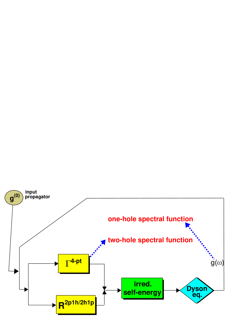
Figure 5: Iteration scheme used to reach self-consistency between the input propagator and the result of the Dyson equation. At each step in the iteration loop new approximations for the one-body propagator (2) and for $\Gamma^{4-pt}$ (16) or $R(\omega)$ are obtained until self-consistency is obtained.

The attractive feature of the SCGF method is not only restricted to the fact that the effects of fragmentation are included in the calculations. Also, solutions for the one-body, two-body and higher-order propagators are generated all at the same time while their mutual influence is taken into account. In addition, the comparison with experimental data can be performed for all ingredients of the calculation yielding important clues for further improvements of the chosen approximation scheme. We stress again that the final self-consistent solutions will not depend in any way on the choice of $\hat{H}_{0}$. Nevertheless, a good choice for the unperturbed propagator $g^{(0)}$ can provide a useful starting point for the first iteration.

The self-consistent propagator $g(\omega)$ enters the construction of higher-order Green’s functions through the use of Bethe-Salpeter equations (BSE). We give a brief description of this approach by considering the three-times polarization propagator,

$$\Pi_{\alpha\beta,\gamma\delta}(t_{1}-t^{\prime},t_{2}-t^{\prime}) = -i~{}\langle\Psi^{A}_{0}|~{}T[c^{{\dagger}}_{\beta}(t_{2})c_{\alpha}(t_{1})c^{{\dagger}}_{\gamma}(t^{\prime})c_{\delta}(t^{\prime})]|\Psi^{A}_{0}\rangle$$ (20)

$$+i~{}\langle\Psi^{A}_{0}|~{}T[c^{{\dagger}}_{\beta}(t_{2})c_{\alpha}(t_{1})]|\Psi^{A}_{0}\rangle\langle\Psi^{A}_{0}|c^{{\dagger}}_{\gamma}(t^{\prime})c_{\delta}(t^{\prime})|\Psi^{A}_{0}\rangle\;,$$

which governs the response of the system to an external perturbation. Working with the equation of motion method, one finds that Eq. (20) is the solution of the following Bethe-Salpeter equation [29, 30].

$$\Pi_{\alpha\beta,\gamma\delta}(t_{1}-t^{\prime},t_{2}-t^{\prime}) = -ig_{\alpha\gamma}(t_{1}-t^{\prime})g_{\delta\beta}(t^{\prime}-t_{2})$$ (21)

$$+~{}\int dt_{3}\int dt_{4}\int dt_{5}\int dt_{6}\sum_{\mu,\nu,\lambda,\eta}g_{\alpha\mu}(t_{1}-t_{3})g_{\nu\beta}(t_{4}-t_{2})$$

$$~{}~{}\times\;K^{ph}_{\mu\nu,\lambda\eta}(t_{3},t_{4};t_{5},t_{6})\;\Pi_{\lambda\eta,\gamma\delta}(t_{5}-t^{\prime},t_{6}-t^{\prime})\;,$$

where the ph irreducible kernel $K^{ph}$, represents all the basic interactions that a quasiparticle and a quasihole can undergo. The latter can be obtained from the exact irreducible self-energy in terms of a functional derivative,

$$K^{ph}_{\alpha\beta,\gamma\delta}(t_{1},t_{2};t_{3},t_{4})~{}=~{}\frac{\delta~{}\Sigma^{\star}_{\alpha\beta}(t_{1}-t_{2})}{\delta~{}g_{\gamma\delta}(t_{3}-t_{4})}\;.$$ (22)

In the language of Feynman diagrams this corresponds to taking the diagrammatic expansion of $\Sigma^{\star}(\omega)$ in terms of the propagator $g(\omega)$ and then generating the contributions to $K^{ph}$ by removing such a sp line in every possible way. Baym and Kadanoff have shown that a conserving approximation of the polarization propagator $\Pi$ is guaranteed if both $K^{ph}$ and $g(\omega)$ are derived from the same approximation of the self-energy (by means of Eqs. (22) and (13), respectively) [29, 31]. From a practical point of view, this approach is not always possible to implement since relatively simple approximations to $\Sigma^{\star}(\omega)$ can generate a very large number of contributions to $K^{ph}$. Fortunately, actual nuclear systems do not necessarily require the inclusion of all of these terms to obtain reasonable results. Nevertheless, the above construction can be used as a guideline to help in choosing the approximation that is suitable for the problem under study. The resulting $K$ will involve an expansion in terms $g(\omega)$ and $\Gamma^{4-pt}$ or $R(\omega)$. The fact that this perturbative expansion is based on the fragmented sp propagator —and not on its unperturbed approximation $g^{(0)}(\omega)$—, acts to renormalize the interaction kernel $K$ and drastically improves the convergence properties, while still allowing to keep track of the relevant physical ingredients in the calculation. The simplest realization of this scheme consists in considering only the bare interaction potential $\hat{V}$ in either the pp or ph channels. The result is the usual random phase approximation (RPA). This approximation is described in more detail in the next section since it is relevant to most of the calculations discussed in this review.

2.4 Ring and ladder approximations

By taking the limit $t_{2}\rightarrow t_{1}^{+}=t$ in Eq. (20), one is left with the usual two-time polarization propagator $\Pi_{\alpha\beta,\gamma\delta}(t-t^{\prime})$. This can be Fourier transformed to its Lehmann representation,

$$\Pi_{\alpha\beta,\gamma\delta}(\omega)~{}=~{}\sum_{n\neq 0}\frac{\langle\Psi^{A}_{0}|c^{{\dagger}}_{\beta}c_{\alpha}|\Psi^{A}_{n}\rangle\langle\Psi^{A}_{n}|c^{{\dagger}}_{\gamma}c_{\delta}|\Psi^{A}_{0}\rangle}{\omega-\left(E^{A}_{n}-E^{A}_{0}\right)+i\eta}~{}-~{}\sum_{n\neq 0}\frac{\langle\Psi^{A}_{0}|c^{{\dagger}}_{\gamma}c_{\delta}|\Psi^{A}_{n}\rangle\langle\Psi^{A}_{n}|c^{{\dagger}}_{\beta}c_{\alpha}|\Psi^{A}_{0}\rangle}{\omega+\left(E^{A}_{n}-E^{A}_{0}\right)-i\eta}\;.$$ (23)

where the poles correspond to the excitation energies $\varepsilon^{\pi}_{n}\equiv E^{A}_{n}-E^{A}_{0}$ of the states of the system whereas the residues contain the corresponding amplitudes to determine transition probabilities from the ground state to these excited states. It is important to note that this information is included for all those states that can be excited by means of a one-body operator, therefore also those with important two-particle$-$two-hole (2p2h) (or even more complex) admixtures. In Eq. (23), the forward- and the backward-going contributions are identical apart from a time reversal transformation.

Analogously, one can define the free ph propagator $\Pi^{f}(\omega)$ by coupling two excitations of particle and hole type, not interacting with each other. Graphically, this corresponds to two dressed sp lines propagating with opposite direction in time. By applying Feynman diagram rules [7], one obtains the following Lehmann representation for $\Pi^{f}(\omega)$,

$$\Pi^{f}_{\alpha\beta,\gamma\delta}(\omega)~{} = ~{}-i\int\frac{d\omega_{1}}{2\pi}(-1)~{}ig_{\alpha\gamma}(\omega+\omega_{1})~{}ig_{\delta\beta}(\omega_{1})$$ (24)

$$= \sum_{n,k}\frac{\langle{\Psi^{A}_{0}}|c^{{\dagger}}_{\beta}|\Psi^{A-1}_{k}\rangle\langle\Psi^{A}_{0}|c_{\alpha}|\Psi^{A+1}_{n}\rangle\;\langle\Psi^{A+1}_{n}|c^{{\dagger}}_{\gamma}|\Psi^{A}_{0}\rangle\langle\Psi^{A-1}_{k}|c_{\delta}|\Psi^{A}_{0}\rangle}{\omega-\left(\varepsilon^{+}_{n}-\varepsilon^{-}_{k}\right)+i\eta}$$

$$~{}-~{}\sum_{n,k}\frac{\langle{\Psi^{A}_{0}}|c^{{\dagger}}_{\gamma}|\Psi^{A-1}_{k}\rangle\langle\Psi^{A}_{0}|c_{\delta}|\Psi^{A+1}_{n}\rangle\;\langle\Psi^{A+1}_{n}|c^{{\dagger}}_{\beta}|\Psi^{A}_{0}\rangle\langle\Psi^{A-1}_{k}|c_{\alpha}|\Psi^{A}_{0}\rangle}{\omega+\left(\varepsilon^{+}_{n}-\varepsilon^{-}_{k}\right)-i\eta}\;,$$

where the forward- and the backward-going contributions describe the propagation of a particle-hole and hole-particle type excitation, respectively.

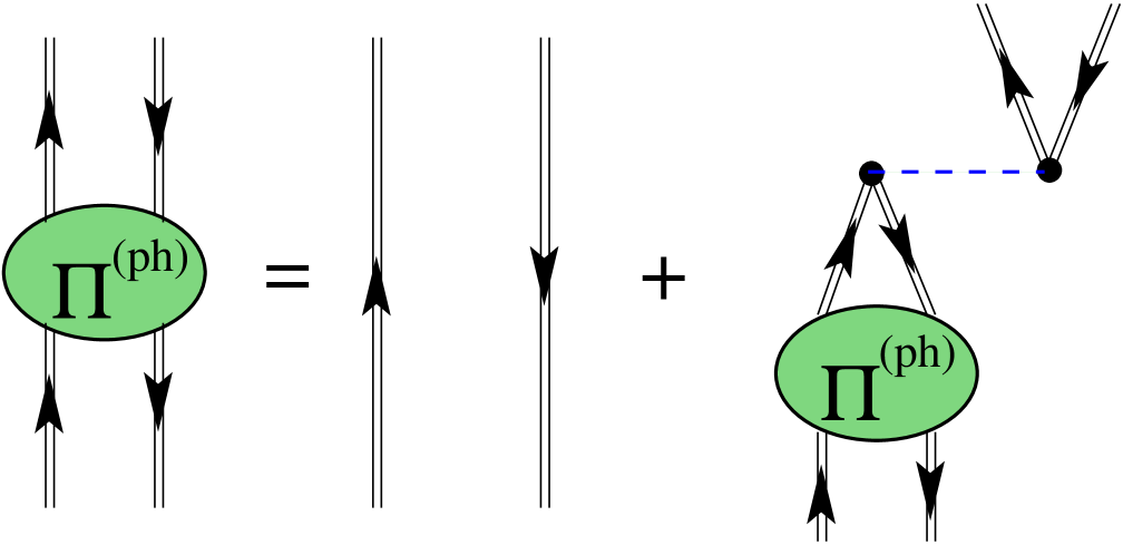
Figure 6: Feynman diagram representation of the DRPA equation for the polarization propagator $\Pi(\omega)$.

In order to account for the collective excitations present in the $A$-body system, one needs to take into account the interactions between the two lines propagating in $\Pi^{f}(\omega)$. The simplest approximation consist in considering only the contribution of the bare two-body potential $\hat{V}$. This corresponds to choosing $K^{ph}_{\alpha\beta,\gamma\delta}=V_{\alpha\delta,\beta\gamma}$ in the Bethe-Salpeter Eq. (21) and results in the standard RPA approximation,

$$\Pi_{\alpha\beta,\gamma\delta}(\omega)~{}=~{}\Pi^{f}_{\alpha\beta,\gamma\delta}(\omega)~{}+~{}\sum_{\mu,\nu,\rho,\epsilon}\Pi^{f}_{\alpha\beta,\mu\nu}(\omega)~{}V_{\mu\epsilon,\nu\rho}~{}\Pi_{\rho\epsilon,\gamma\delta}(\omega)\;,$$ (25)

which is depicted in Fig. 6 in terms of Feynman diagrams. Equation (25) implicitly generates a series of diagrams in which the particle and the hole interact any number of times. The resulting expansion is depicted in Figs. 7 and 8, in terms of $g^{(0)}(\omega)$ propagators.

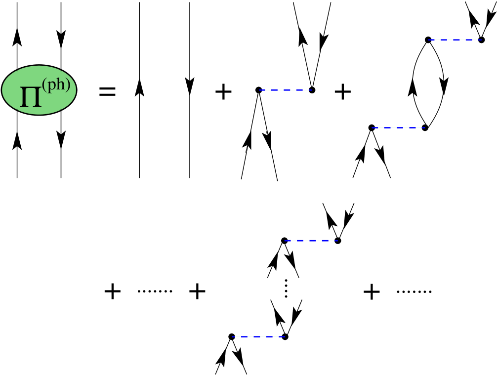
Figure 7: Diagrammatic expansion of the ph propagator $\Pi(\omega)$ in TDA. An implicit time ordering is intended for these diagrams. Dressing all the sp lines would result in the DTDA.

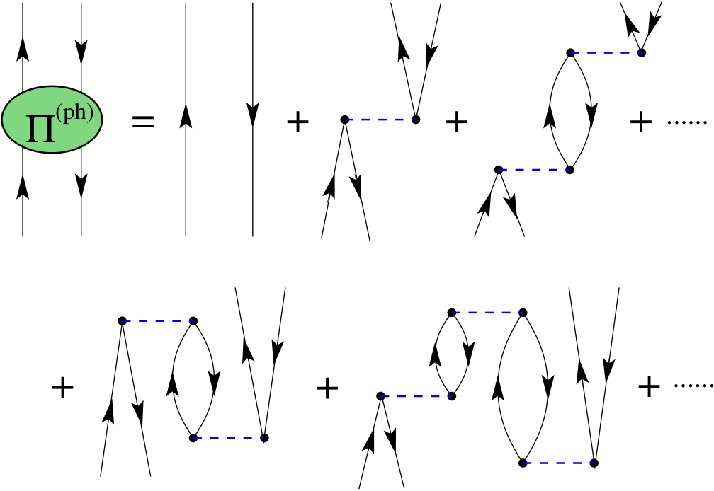
Figure 8: Diagrammatic expansion of the ph propagator $\Pi(\omega)$ in RPA. This contains the whole phTDA series plus diagrams involving the inversion of the propagation time. Dressing all the sp lines results in the DRPA.

A simpler approximation consists in considering only the forward-going propagation in Eq. (25), i. e. to include only the first term of Eq. (24). This corresponds to the so-called dressed Tamm-Dancoff approximation (DTDA), depicted in Fig. 7 (where an explicit time ordering is assumed and the dressing of sp Green’s functions is implied). When the full $\Pi^{f}(\omega)$ is employed in Eq. (25), one obtains the dressed random phase approximation (DRPA). The relevant diagrammatic expansion is the one given in Fig. 8. Clearly, the whole TDA series is contained in the RPA one. Besides this contribution, the backward-going component of $\Pi^{f}(\omega)$ generates diagrams containing more that a single ph excitation at each time. These refer to contributions in which additional intermediate ph states are present and eventually annihilated by two-body interactions. Consistent with the aim of performing a self-consistent calculation, Eqs. (24) and (25) have been formulated in terms of the full, dressed, sp propagator $g(\omega)$ given in Eq. (2). When an unperturbed, IPM, Green’s function $g^{0}(\omega)$ (8) is used as input, the approximations described here reduce to the standard TDA and RPA results [33].

In general, the interparticle distance between nucleons inside the nucleus is of the order of the nucleon size itself so that the nuclear medium can be considered a rather dense system. Besides, the nuclear effective interaction remains substantial. A natural consequence is that the “vacuum fluctuation” contributions that are included in the RPA expansion play an important role in the description of nuclear systems. It must be realized, however, that the intermediate n-particle–n-hole excitations depicted in Fig. 8 do not represent all the possible diagrams related by Pauli exchange of two sp lines. The philosophy underlying the use of RPA relies on the assumption that the corrections coming from Pauli correlations sum up in a random way and tend to cancel each other (whence the name “random phase”) [34] - [36]. As a result, the Pauli principle may only be violated slightly and the improvement obtained by including RPA correlations is generally more relevant. In such cases, the RPA is a useful approximation. It must be kept in mind, however, that in systems containing strong collective and/or pairing correlations the effects of Pauli violation may sum up in a coherent way, invalidating the standard RPA approach. Typically this situation is signaled by the appearence of a pair of complex eigenvalues of Eq. (25) together with diverging solutions for the ph spectroscopic amplitudes.

We also note that using dressed propagators $g(\omega)$ in Eq. (24) results in including implicitly diagrams that go beyond the bare 1p1h configurations already at the level of $\Pi^{f}(\omega)$. This is due to the self-energy insertions in each particle and hole line. The fragmentation of $g(\omega)$ acts once again to renormalize the free propagator $\Pi^{f}(\omega)$ thereby adding stability to the DRPA approach, as compared the the bare RPA one.

The saturation energy of nuclear matter, as well as the spectral distribution at high missing energies, is governed by short-range effects and two-body correlations. Moreover, some particular nuclei present strong pairing effects. In these cases, one is faced with two-body correlations in the system and a proper description of the physics calls for a direct evaluation of the interaction between two particles in the medium. From the experimental point of view, the ideal approach to study such effects is represented by addition or removal of the correlated pair (see Sec. 3). The information required to study such processes are also contained in the four-point Green’s function, $g^{4-pt}$. One can define the two-particle propagator $g^{II}(t-t^{\prime})$ as a two-time reduction of Eq. (15)

$$g^{II}_{\alpha\beta,\gamma\delta}(t-t^{\prime})~{}=~{}g^{4-pts}_{\alpha\beta,\gamma\delta}(t,t^{+};t^{\prime}{}^{+},t^{\prime})\;.$$ (26)

Its Lehmann representation,

$$g^{II}_{\alpha\beta,\gamma\delta}(\omega)=\sum_{n}\frac{\langle{\Psi^{A}_{0}}|c_{\beta}c_{\alpha}|{\Psi^{A+2}_{n}}\rangle\;\langle{\Psi^{A+2}_{n}}|c^{{\dagger}}_{\gamma}c^{{\dagger}}_{\delta}|{\Psi^{A}_{0}}\rangle}{\omega-\left(E^{A+2}_{n}-E^{A}_{0}\right)+i\eta}-\sum_{k}\frac{\langle{\Psi^{A}_{0}}|c^{{\dagger}}_{\gamma}c^{{\dagger}}_{\delta}|{\Psi^{A-2}_{k}}\rangle\;\langle{\Psi^{A-2}_{k}}|c_{\beta}c_{\alpha}|{\Psi^{A}_{0}}\rangle}{\omega-\left(E^{A}_{0}-E^{A-2}_{k}\right)-i\eta}\;.$$ (27)

contains the spectroscopic amplitudes for a transition from the ground state $|{\Psi^{A}_{0}}\rangle$ to the eigenstates of the systems with $A\pm 2$ particles and the respective excitation energies with respect to $E^{A}_{0}$.

As for the polarization propagator, the zero-order contribution consists of two noninteracting lines, propagating in the same time direction. The Lehmann representation for the dressed case is given by

$$g^{II,f}_{\alpha\beta,\gamma\delta}(\omega) = -i\int\frac{d\omega_{1}}{2\pi}~{}ig_{\alpha\gamma}(\omega-\omega_{1})~{}ig_{\beta\delta}(\omega_{1})$$ (28)

$$= ~{}\sum_{n_{1},n_{2}}~{}\frac{\langle\Psi^{A}_{0}|c_{\beta}|\Psi^{A+1}_{n_{2}}\rangle\langle\Psi^{A}_{0}|c_{\alpha}|\Psi^{A+1}_{n_{1}}\rangle\;\langle\Psi^{A+1}_{n_{1}}|c^{{\dagger}}_{\gamma}|\Psi^{A}_{0}\rangle\langle\Psi^{A+1}_{n_{2}}|c^{{\dagger}}_{\delta}|\Psi^{A}_{0}\rangle}{\omega-\left(\varepsilon^{+}_{n_{1}}+\varepsilon^{+}_{n_{2}}\right)+i\eta}$$

$$~{}~{}-~{}\sum_{k_{1},k_{2}}~{}\frac{\langle{\Psi^{A}_{0}}|c^{{\dagger}}_{\gamma}|\Psi^{A-1}_{k_{1}}\rangle\langle{\Psi^{A}_{0}}|c^{{\dagger}}_{\delta}|\Psi^{A-1}_{k_{2}}\rangle\;\langle\Psi^{A-1}_{k_{2}}|c_{\beta}|\Psi^{A}_{0}\rangle\langle\Psi^{A-1}_{k_{1}}|c_{\alpha}|\Psi^{A}_{0}\rangle}{\omega-\left(\varepsilon^{-}_{k_{1}}+\varepsilon^{-}_{k_{2}}\right)-i\eta}\;,$$

where the forward and backward parts refer to the (independent) propagation of two particle and two hole lines, respectively. The two-particle dressed RPA (ppDRPA) equation is given by

$$g^{II}_{\alpha\beta,\gamma\delta}(\omega)~{}=~{}\left(g^{II,f}_{\alpha\beta,\gamma\delta}(\omega)-g^{II,f}_{\beta\alpha,\gamma\delta}(\omega)\right)~{}+~{}\frac{1}{2}\sum_{\mu\nu\rho\varepsilon}g^{II,f}_{\alpha\beta,\mu\nu}(\omega)\;V_{\mu\nu,\rho\epsilon}\;g^{II}_{\rho\epsilon,\gamma\delta}(\omega)\;,$$ (29)

where the symmetry factor $\frac{1}{2}$ is required by the Feynman rules [7].

Equation (29) is depicted in terms of Feynman diagrams in Fig. 9 and generates a series of ladder diagrams in a similar fashion as higher order terms are generated in Fig. 8. We note that this approach is equivalent to computing the two-body wave function of a pair propagating inside the medium, while the Pauli blocking effects are being taken into account in a similar fashion to the Bethe-Goldstone equation [37, 38]. The ppDRPA has two advantages over that approximation. First the details of the sp particle fragmentation, included in Eq. (28), allows for a partial propagation below the Fermi level. This is due to the fact that in the correlated system the Fermi sea is partially depleted. The dressed result therefore corresponds to propagation with respect to the correlated ground state and not the IPM as in the Bethe-Goldstone equation. Second, the advantage of an RPA approach over the TDA one is that it accounts for the propagation of hh excitations in the ground state of the system. Without this latter feature, the resulting self-energy would not yield the fragmentation of the sp strength below the Fermi energy. As in the ph case, the corresponding ppDTDA approximation is obtained by considering propagation only in one time direction. This corresponds to including only the first term from the left of Eq.(28) into Eq. (29) when solving for the pp part of $g^{II}$, therefore neglecting the hh contributions.

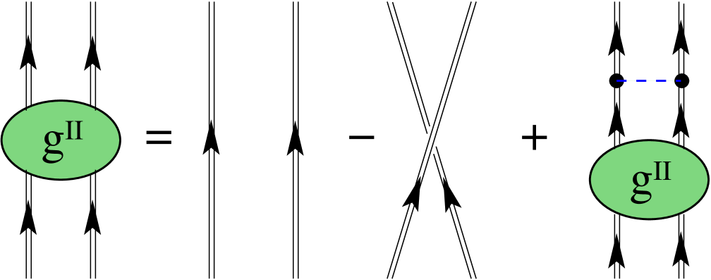
Figure 9: DRPA (ladder) equation for the two-particle propagator $g^{II}(\omega)$.

In general, both the two-particle and the polarization propagator represent different time orderings of the same 4-points Green’s function, see Eqs. (20) and (26). By making use of Eq. (14) and (17) one can include the effects of ph or pp(hh) motion directly in the nuclear self-energy.

3 Relation to experimental data

In this section we will explore the connection between the information contained in various propagators and experimental data. Detailed work on this subject has been presented in Ref. [39] and we refer to that paper for a discussion of the relation between elastic nucleon scattering and the particle part of the sp propagator. In this paper the focus is on the experimental properties that are probed by the removal of nucleons. Nevertheless, it will be necessary within the theoretical treatment to simultaneously consider the addition and removal aspects of the propagators as discussed in Sec. 2. Before making this connection it is useful to demonstrate that the Dyson equation (Eq. (13) ) yields a Schrödinger-like equation with corresponding interpretation of the removal or addition amplitudes appearing in Eq. (3). We will discuss here the case when the spectrum for the $A\pm 1$-particle system near the Fermi energy involves discrete bound states which applies to a finite system like a nucleus. An appropriate form of the Lehmann representation in this case is given by

$$g_{\alpha\beta}(\omega)=\sum_{n}\frac{\left\langle\Psi^{A}_{0}\right|c_{\alpha}\left|\Psi^{A+1}_{n}\right\rangle\left\langle\Psi^{A+1}_{n}\right|c^{\dagger}_{\beta}\left|\Psi^{A}_{0}\right\rangle}{E-\varepsilon^{+}_{n}+i\eta}+\int_{\varepsilon^{+}_{T}}^{\infty}d\varepsilon^{+}_{\nu}\frac{\left\langle\Psi^{A}_{0}\right|c_{\alpha}\left|\Psi^{A+1}_{\nu}\right\rangle\left\langle\Psi^{A+1}_{\nu}\right|c^{\dagger}_{\beta}\left|\Psi^{A}_{0}\right\rangle}{E-\varepsilon^{+}_{\nu}+i\eta}$$ (30)

$$+\sum_{k}\frac{\left\langle\Psi^{A}_{0}\right|c^{\dagger}_{\beta}\left|\Psi^{A-1}_{k}\right\rangle\left\langle\Psi^{A-1}_{k}\right|c_{\alpha}\left|\Psi^{A}_{0}\right\rangle}{E-\varepsilon^{-}_{k}-i\eta}+\int^{\varepsilon^{-}_{T}}_{-\infty}d\varepsilon^{-}_{\kappa}\frac{\left\langle\Psi^{A}_{0}\right|c^{\dagger}_{\beta}\left|\Psi^{A-1}_{\kappa}\right\rangle\left\langle\Psi^{A-1}_{\kappa}\right|c_{\alpha}\left|\Psi^{A}_{0}\right\rangle}{E-\varepsilon^{-}_{\kappa}-i\eta},\hskip 2.84544pt$$

where the continuum energy spectrum for the $A\pm 1$ systems has been included and the corresponding energy thresholds are denoted by $\varepsilon^{\pm}_{T}$. A change of integration variable was also used to obtain this form of the Lehmann representation introducing the integration variables for the continuum energies in the form $\varepsilon^{+}_{\nu}=E^{A+1}_{\nu}-E^{A}_{0}$ and $\varepsilon^{-}_{\kappa}=E^{A}_{0}-E^{A-1}_{\kappa}$ , respectively. For the unperturbed propagator one will encounter sp energies associated with $H_{0}$ that are different from the poles of $g(\omega)$. By exploring the equations of motion of the two-body propagator, it is possible to show that a Lehmann representation also exists for the exact self-energy and has different poles from the ones for $g(\omega)$ [6]. These features can be used to identify the residues of discrete solutions in the Lehmann representation from the Dyson equation. In practice, one may proceed with taking the following limit of the Dyson equation for the case of the hole part of the propagator (without generating contributions from the poles in the self-energy or the noninteracting propagator)

$$\lim_{\omega\to\varepsilon^{-}_{k}}(\omega-\varepsilon^{-}_{k})\ \Big{\{}g_{\alpha\beta}(\omega)=g_{\alpha\beta}^{(0)}(\omega)+\sum_{\gamma\delta}g_{\alpha\gamma}^{(0)}(\omega)\ \Sigma_{\gamma\delta}^{\star}(\omega)\ g_{\delta\beta}(\omega)\ \Big{\}}.$$ (31)

This limit process generates an eigenvalue equation of the following kind

$$z^{k-}_{\alpha}=\sum_{\gamma,\delta}\ g^{(0)}_{\alpha\gamma}(\varepsilon^{-}_{k})\ \Sigma^{\star}_{\gamma\delta}(\varepsilon^{-}_{k})\ z^{k-}_{\delta},$$ (32)

where

$$z^{k-}_{\alpha}=\left\langle\Psi^{A-1}_{k}\right|c_{\alpha}\left|\Psi^{A}_{0}\right\rangle.$$ (33)

Since the Dyson equation can be written in any sp basis, one may choose the coordinate representation with $sp$ quantum numbers ${\bf r},m$ for the position and spin projection, respectively, to solve Eq. (32). In this basis one obtains

$$z^{k-}_{{\bf r}m}=\sum_{m_{1},m_{2}}\int\!\!d^{3}r_{1}\int\!\!d^{3}r_{2}\ g^{(0)}_{{\bf r}m~{}{\bf r}_{1}m_{1}}(\varepsilon^{-}_{k})\ \Sigma^{\star}_{{\bf r}_{1}m_{1}~{}{\bf r}_{2}m_{2}}(\varepsilon^{-}_{k})\ z^{k-}_{{\bf r}_{2}m_{2}}.$$ (34)

Equation (34) can be rearranged by inverting the unperturbed propagator according to

$$\sum_{m}\int\!\!d^{3}r\left\langle{\bf r^{\prime}}m^{\prime}\right|\varepsilon^{-}_{k}-H_{0}\left|{\bf r}m\right\rangle g^{(0)}_{{\bf r}m~{}{\bf r}_{1}m_{1}}(\varepsilon^{-}_{k})=\delta_{m^{\prime},m_{1}}\delta({\bf r}^{\prime}-{\bf r}_{1}).$$ (35)

The corresponding operation on $z^{k-}_{{\bf r}m}$ yields

$$\sum_{m}\int\!\!d^{3}r\ \left\langle{\bf r^{\prime}}m^{\prime}\right|\varepsilon^{-}_{k}-H_{0}\left|{\bf r}m\right\rangle z^{k-}_{{\bf r}m}=\left\{\varepsilon^{-}_{k}+\frac{\hbar^{2}\nabla^{\prime}{}^{2}}{2m}-U({\bf r}^{\prime})\right\}z^{k-}_{{\bf r}^{\prime}m^{\prime}},$$ (36)

where $U$ is assumed to be local and spin-independent for simplicity. Combining these results yields the explicit cancellation of the auxiliary potential $U$ and the following result

$$-\frac{\hbar^{2}\nabla^{2}}{2m}z^{k-}_{{\bf r}m}+\sum_{m_{1}}\int\!\!d^{3}r_{1}\ \Sigma^{\prime}{}^{\star}_{{\bf r}m~{}{\bf r}_{1}m_{1}}(\varepsilon_{k})z^{k-}_{{\bf r}_{1}m_{1}}=\varepsilon^{-}_{k}z^{k-}_{{\bf r}m},$$ (37)

where the notation $\Sigma^{\prime}{}^{\star}$ has been used to signify that the $U$ contribution has been removed. This equation has the form of a Schrödinger equation with a nonlocal potential which is represented by the self-energy $\Sigma^{\prime}{}^{\star}$. Note that an eigenvalue $\varepsilon^{-}_{k}$ can only be obtained when it coincides with the energy argument of the self-energy. An important difference with the ordinary Schrödinger equation is related to the normalization of the quasihole “eigenfunctions” $z^{k-}_{{\bf r}m}$. The appropriate normalization condition is obtained by considering terms beyond the pole contribution in the Dyson equation. This result is most conveniently expressed in terms of the sp state (itself normalized to 1) which corresponds to the quasihole wave function $z^{n}_{{\bf r}m}$. In other words, one can use the eigenstate which diagonalizes Eq. (37) with eigenvalue $\varepsilon^{-}_{k}$, to express the normalization condition. Assigning the notation $\alpha_{qh}$ to this sp state, one obtains with $z^{k-}_{\alpha_{qh}}=\left\langle\Psi^{A-1}_{k}\right|c_{\alpha_{qh}}\left|\Psi^{A}_{0}\right\rangle$

$$\mid z^{k-}_{\alpha_{qh}}\mid^{2}=\bigg{(}{1-\frac{\partial\Sigma^{\prime}{}^{\star}_{\alpha_{qh},\alpha_{qh}}(E)}{\partial E}\bigg{|}_{\varepsilon^{-}_{k}}}\bigg{)}^{-1},$$ (38)

where the subscript $qh$ refers to the quasihole nature of this state and the fact that for states very near to the Fermi energy with quantum numbers corresponding to fully occupied mean-field states the normalization yields a number of order 1. This result is equivalent to the definition given in Eq. (7).

3.1 Spectroscopic strength from the $(e,e^{\prime}p)$ reaction

In order to make the connection with experimental data obtained from knockout reactions, it is useful to consider the response of a system to a weak probe. The hole spectral function introduced in Sec. 2 can be experimentally “observed” in so-called knockout reactions. The general idea is to transfer a large amount of momentum and energy to a proton of a bound nucleus in the ground state. The proton is then ejected from the system, and one ends up with a fast-moving particle and a bound $(A-1)$-particle system. By observing the momentum of the ejected particle it is then possible the reconstruct the spectral function of the system, provided that the interaction between the ejected particle and the remainder is sufficiently weak or treated in a controlled fashion, e. g. by constraining this treatment with information from other experimental data.

We assume that the $A$-particle system is initially in its ground state,

$$\left|\Psi_{i}\right\rangle=\left|\Psi^{A}_{0}\right\rangle,$$ (39)

and makes a transition to a final $A$-particle eigenstate

$$\left|\Psi_{f}\right\rangle=a^{\dagger}_{\bm{p}}\left|\Psi^{A-1}_{n}\right\rangle,$$ (40)

composed of a bound $(A-1)$-particle eigenstate, $\left|\Psi^{A-1}_{n}\right\rangle$, and a particle with momentum $\bm{p}$.

For simplicity we consider the transition matrix elements for a scalar external probe

$$\rho({\bm{q}})=\sum_{j=1}^{A}\exp{(i{\bm{q}}\cdot{\bm{r}}_{j})},$$ (41)

which transfers momentum $\bm{q}$ to a particle. Suppressing other possible sp quantum numbers, like e.g. spin, the second-quantized form of this operator is given by

$$\hat{\rho}({\bm{q}})=\sum_{\bm{p},\bm{p}^{\prime}}\left\langle\bm{p}\right|\exp{(i{\bm{q}}\cdot{\bm{r}})}\left|\bm{p}^{\prime}\right\rangle a^{\dagger}_{\bm{p}}a_{\bm{p}^{\prime}}=\sum_{\bm{p}}a^{\dagger}_{\bm{p}}a_{{\bm{p}}-{\bm{q}}}.$$ (42)

The transition matrix element now becomes

$$\left\langle\Psi_{f}\right|\hat{\rho}({\bm{q}})\left|\Psi_{i}\right\rangle = \sum_{\bm{p}^{\prime}}\left\langle\Psi^{A-1}_{n}\right|a_{\bm{p}}a^{\dagger}_{\bm{p}^{\prime}}a_{\bm{p}^{\prime}-\bm{q}}\left|\Psi^{A}_{0}\right\rangle=\sum_{\bm{p}^{\prime}}\left\langle\Psi^{A-1}_{n}\right|\delta_{\bm{p}^{\prime},\bm{p}}a_{\bm{p}^{\prime}-\bm{q}}+a^{\dagger}_{\bm{p}^{\prime}}a_{\bm{p}^{\prime}-\bm{q}}a_{\bm{p}}\left|\Psi^{A}_{0}\right\rangle$$ (43)

$$\approx \left\langle\Psi^{A-1}_{n}\right|a_{{\bm{p}}-{\bm{q}}}\left|\Psi^{A}_{0}\right\rangle.$$

The last line is obtained in the so-called Impulse Approximation, where it is assumed that the ejected particle is the one that has absorbed the momentum from the external field. This is a very good approximation whenever the momentum ${\bm{p}}$ of the ejectile is much larger than typical momenta for the particles in the bound states; the neglected term in Eq. (43) is then very small, as it involves the removal of a particle with momentum ${\bm{p}}$ from $\left|\Psi^{A}_{0}\right\rangle$.

There is one other assumption in the derivation: the fact that the final eigenstate of the $A$-particle system was written in the form of Eq. (40), i.e. a plane-wave state for the ejectile on top of an $(A-1)$-particle eigenstate. This is again a good approximation if the ejectile momentum is large enough, as can be understood by rewriting the Hamiltonian in the $A$-particle system as

$$H_{A}=\sum_{i=1}^{A}\frac{{\bm{p}}^{2}_{i}}{2m}+\sum_{i<j=1}^{A}V(i,j)=H_{A-1}+\frac{{\bm{p}}^{2}_{A}}{2m}+\sum_{i=1}^{A-1}V(i,A).$$ (44)

The last term in Eq. (44) represents the Final State Interaction, or the interaction between the ejected particle $A$ and the other particles $1\dots A-1$. If the relative momentum between particle $A$ and the others is large enough their mutual interaction can be neglected, and $H_{A}\approx H_{A-1}+\bm{p}^{2}_{A}/2m$. The result given by Eq. (43) is called the Plane Wave Impulse Approximation or PWIA knock-out amplitude, for obvious reasons, and is precisely a removal amplitude (in the momentum representation) appearing in the Lehmann representation of the sp propagator (see Eq. (3) ).

The cross section of the knock-out reaction, where the momentum and energy of the ejected particle and the probe are either measured or known, is according to Fermi’s golden rule proportional to

$$d\sigma\sim\sum_{n}\delta(\omega+E_{i}-E_{f})|\left\langle\Psi_{f}\right|\hat{\rho}({\bm{q}})\left|\Psi_{i}\right\rangle|^{2},$$ (45)

where the energy-conserving $\delta$-function contains the energy transfer $\omega$ of the probe, and the initial and final energies of the system are $E_{i}=E^{A}_{0}$ and $E_{f}=E^{A-1}_{n}+{\bm{p}}^{2}/2m$, respectively. Note that the internal state of the residual $A-1$ system is not measured, hence the summation over $n$ in Eq. (45). Defining the missing momentum $\bm{p}_{miss}$ and missing energy $E_{miss}$ of the knock-out reaction as

$$\bm{p}_{miss}={\bm{p}}-{\bm{q}}$$ (46)

and

$$E_{miss}={\bm{p}}^{2}/2m-\omega=E^{A}_{0}-E^{A-1}_{n},$$ (47)

respectively, the PWIA knock-out cross section can be rewritten as

$$d\sigma \sim \sum_{n}\delta(E_{miss}-E^{A}_{0}+E^{A-1}_{n})|\left\langle\Psi^{A-1}_{n}\right|a_{\bm{p}_{miss}}\left|\Psi^{A}_{0}\right\rangle|^{2}$$ (48)

$$= S_{h}(\bm{p}_{miss},E_{miss}).$$

The PWIA cross section is therefore exactly proportional to the hole spectral function defined in Eq. (4). This is of course only true in the PWIA, but when the deviations of the impulse approximation and the effects of the final state interaction are under control, it is possible to obtain precise experimental information on the hole spectral function of the system under study. Although the actual (e,e^′p) experiments involve more complicated one-body excitation operators than the one considered here in this simple example, the basic conclusions are not altered [11].

An even more realistic description of the proton knockout reaction again identifies the external electron probe and the corresponding virtual photon as represented by a one-body excitation operator.

$$\hat{O}=\sum_{\alpha\beta}\left\langle\alpha\right|O\left|\beta\right\rangle a^{\dagger}_{\alpha}a_{\beta}.$$ (49)

The response of the system to such an external excitation operator is described by the polarization propagator which has a Lehmann representation given by Eq. (23). The transition probability induced by $\hat{O}$ from the ground state to an excited state is given by

$$\left|\left\langle\Psi^{A}_{n}\right|\hat{O}\left|\Psi^{A}_{0}\right\rangle\right|^{2}=\sum_{\alpha\beta}\sum_{\gamma\delta}\left\langle\gamma\right|O\left|\delta\right\rangle\left\langle\Psi^{A}_{n}\right|a^{\dagger}_{\gamma}a_{\delta}\left|\Psi^{A}_{0}\right\rangle\left\langle\alpha\right|O\left|\beta\right\rangle^{*}\left\langle\Psi^{A}_{n}\right|a^{\dagger}_{\alpha}a_{\beta}\left|\Psi^{A}_{0}\right\rangle^{*}.$$ (50)

This result demonstrates that the numerator of the first term in Eq. (23) contains the relevant transition amplitudes for a given state $n$ to evaluate this transition probability. In general, there are important correlations between the ph states, in particular at low energy where collective surface vibrations and giant resonances occur. At higher excitation energy and momentum transfer, these collective coherence effects tend to disappear. In this domain, one may therefore write the polarization propagator as the product of two dressed sp propagators as in Eq. (24). Replacing $\Pi$ by this dressed $\Pi^{f}$ one neglects contributions where the particle and hole interact but includes all other correlations associated with the full dressing of the removed particle in terms of the corresponding removal amplitude (or spectral function) and the corresponding dressing of the particle that will ultimately be detected in the (e,e^′p) experiment. The wave function of this dressed particle corresponds to the addition amplitude in coordinate space and can be associated with an optical model wave function [39]. From this analysis it becomes therefore clear that one may use empirical information associated with the elastic scattering of protons in terms of optical potentials to describe this wave function of the outgoing proton. Clearly, it is this interpretation that clarifies the assumptions that underly the standard analyis of the (e,e^′p) reaction [12] - [17]. In the practical analysis of an (e,e^′p) experiment it is conventional to find a local potential well (mostly of Woods-Saxon type) which will generate a sp state at the removal energy for the transition that is studied. This state is further required to provide the best possible fit to the experimental momentum dependence of the cross section (with proper inclusion of complications due to electron and proton distortion) [12] - [17]. The overall factor necessary to bring the resulting calculated cross section into agreement with the experimental data, can then be interpreted as the spectroscopic factor corresponding to the “experimental” quasihole wave function according to Eq.(38).

The resulting cross sections obtained at the NIKHEF facility are shown for four different nuclei in Fig. 10 [15].

Figure 10: Momentum distributions for various nuclei obtained from the (e,e^′p) reaction performed at NIKHEF [15].

It is important to realize that the shapes of the wave functions in momentum space correspond closely to the ones expected on the basis of a standard Woods-Saxon potential well (or more involved mf wave functions). This is itself an important observation since the (e,e^′p) reaction probes the interior of the nucleus, a feat not available with hadronically induced reactions.

While the shapes of the valence nucleon wave functions correspond to the basic ingredients expected on the basis of years of nuclear structure physics experience, there is a significant departure with regard to the integral of the square of these wave functions. This quantity is of course the spectroscopic factor and is shown in Fig. 11 for the data obtained at NIKHEF [15].

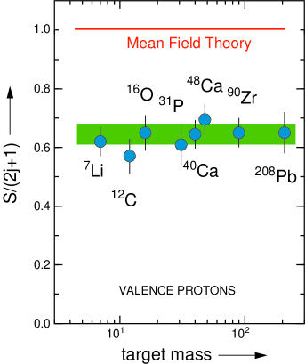
Figure 11: Spectroscopic factors from the (e,e^′p) reaction as a function of target mass. Data have been obtained at the NIKHEF facility [15].

The results shown in Fig. 11 indicate that there is an essentially global reduction of the sp strength of about 35 % which needs to be explained by the theoretical calculations. This depletion is somewhat less for the strength associated with slightly more bound levels. An additional feature obtained in the (e,e^′p) reaction is the fragmentation pattern of these more deeply bound orbitals in nuclei. This pattern is such that single isolated peaks are obtained only in the immediate vicinity of the Fermi energy whereas for more deeply bound states a stronger fragmentation of the strength is obtained with larger distance from $\varepsilon_{F}$. This is beautifully illustrated by the (e,e^′p) data from Quint [40] (see Sec. 5). Whereas the $3s_{1/2}$ orbit exhibits a single peak, there is a substantial fragmentation of the $1f$ strength as indicated in this figure. Additional information about the occupation number of the former orbit is also available and can be obtained by analyzing elastic electron scattering cross sections of neighboring nuclei [41]. The actual occupation number for the $3s_{1/2}$ proton orbit obtained from this analysis is about 10% larger than the quasihole spectroscopic factor [42, 43] and therefore corresponds to 0.75. All these features of the strength need to be explained theoretically. This will be attempted in the material covered in later sections.

3.2 Information from the (e,e^′2N) reaction

Suggestions to explore SRC in two-nucleon emission reactions go back to the work of Gottfried [44]. More recently, theoretical work has focused on the possibility to utilize the (e,e^′2N) reaction to probe nucleon-nucleon correlations [45] - [47]. Practical descriptions of this reaction have been developed by the Pavia group [48] - [51]. Proceeding in a similar vein as in the analysis of the (e,e^′p) reaction, which yields information about the one-nucleon (removal) spectral function, one may hope to learn about the two-nucleon (removal) spectral function in two-nucleon emission processes. The emission of two protons is particularly promising for studies of SRC since the effect of meson-exchange currents and isobars is not expected to dominate the cross section under suitable kinematic conditions [49].

Experiments have been carried out for ¹²C [52] and ¹⁶O (discussed in more detail in Sec. 5.7) to explore the feasibility of gaining insight into nucleon-nucleon correlations in finite nuclei using the (e,e^′pp) reaction. Triple coincidence measurements involving protons with large initial momenta seem particularly suitable to provide information on SRC. The scattered electron is then expected to transfer a virtual photon to one of these two protons which have large and opposite momenta and therefore a relatively small center-of-mass momentum. This strong correlation results from hard collisions due to the strong repulsive core of the NN interaction. When one of the protons is removed by the absorption of the virtual photon, its partner will also leave the nucleus under the assumption that the energy transfer is mainly to the hit pair (the residual nucleus stays at a low excitation energy) [48]. It is therefore hoped that, if the coupling of the virtual photon to one nucleon is the dominant mechanism, the (e,e^′pp) process may be exploited as a useful tool to investigate these short-range correlation effects (see also Ref. [53]).

One of the goals of triple coincidence measurements is to illuminate the features of the interaction between two nucleons before their knockout of the nucleus and their subsequent detection. Early experiments on ¹²C employing the (e,e^′pp) reaction already assumed in the analysis of the data obtained at NIKHEF [54, 48] that the virtual photon is coupled to one of the detected protons. This approximation can be understood by considering the transition matrix element of the nuclear charge operator in momentum space

$$\hat{\rho}(\bm{q})=e\sum_{\bm{p}^{\prime}}a^{\dagger}_{\bm{p}^{\prime}+\bm{q}}a_{\bm{p}^{\prime}}$$ (51)

(with spin implicit in the summation) between the initial state $\left|\Psi^{A}_{0}\right\rangle$ and an approximate final state of the form

$$\left|\Psi_{final}\right\rangle=a^{\dagger}_{\bm{p}_{1^{\prime}}}a^{\dagger}_{\bm{p}_{2^{\prime}}}|\Psi^{A-2}_{n}\rangle.$$ (52)

This final state contains two plane wave protons and an exact state $\left|\Psi_{n}^{A-2}\right\rangle$ for the system with two protons removed. In calculating the matrix elements of the transition charge operator one obtains

$$\langle\Psi_{final}|{\hat{\rho}}(\bm{q})|\Psi^{A}_{0}\rangle=\langle\Psi^{A-2}_{n}|a_{\bm{p}^{\prime}_{2}}a_{\bm{p}^{\prime}_{1}-\bm{q}}|\Psi^{A}_{0}\rangle+\langle\Psi^{A-2}_{n}|a_{\bm{p}^{\prime}_{2}-\bm{q}}a_{\bm{p}^{\prime}_{1}}|\Psi^{A}_{0}\rangle,$$ (53)

assuming that one of the detected protons absorbs the momentum $\bm{q}$. To obtain the contribution to the cross section one requires the square of this matrix element. This yields four terms, each representing a particular term of Eq. (54) for the two-nucleon spectral function. An important ingredient in the description of the two-nucleon knock-out reaction is the two-hole spectral function defined by

$$S^{hh}(\bm{p}_{1},\bm{p}_{2},\bm{p}_{1^{\prime}},\bm{p}_{2^{\prime}},\omega)=\sum_{n}\langle\Psi^{A}_{0}|a^{\dagger}_{\bm{p}_{1^{\prime}}}a^{\dagger}_{\bm{p}_{2^{\prime}}}|\Psi^{A-2}_{n}\rangle\langle\Psi^{A-2}_{n}|a_{\bm{p}_{1}}a_{\bm{p}_{2}}|\Psi^{A}_{0}\rangle\delta(\omega-(E^{A}_{0}-E^{A-2}_{n}))\;,$$ (54)

where $\left|\Psi^{A}_{0}\right\rangle$ may denote the ($0^{+}$) ground state of the target system (for example ¹⁶O) and $\left|\Psi^{A-2}_{n}\right\rangle$ the $n$-th excited state of the residual nucleus (¹⁴C). In Eq. (54), $a^{\dagger}_{{\bf p}}$ ($a_{{\bf p}}$) represent the addition (removal) operators of a nucleon with momentum ${\bf p}$ (spin and isospin are implicit). It is therefore clear that the appropriate expression for the transition probability is to consider the quantity

$$\hat{S}(\bm{p}^{\prime}_{1},\bm{p}^{\prime}_{2},E) = S^{hh}(\bm{p}^{\prime}_{1}-\bm{q},\bm{p}^{\prime}_{2},\bm{p}^{\prime}_{1}-\bm{q},\bm{p}^{\prime}_{2},E)+S^{hh}(\bm{p}^{\prime}_{1}-\bm{q},\bm{p}^{\prime}_{2},\bm{p}^{\prime}_{1},\bm{p}^{\prime}_{2}-\bm{q},E)$$ (55)

$$+ S^{hh}(\bm{p}^{\prime}_{1},\bm{p}^{\prime}_{2}-\bm{q},\bm{p}^{\prime}_{1}-\bm{q},\bm{p}^{\prime}_{2},E)+S^{hh}(\bm{p}^{\prime}_{1},\bm{p}^{\prime}_{2}-\bm{q},\bm{p}^{\prime}_{1},\bm{p}^{\prime}_{2}-\bm{q},E)\;,$$

where the vector $\bm{q}$ is the momentum of the virtual photon.

More realistic implementations of this reaction model naturally require the consideration of the distortion effects of the outgoing particles. Nevertheless, this simple representation of the reaction clarifies the intrinsic importance of two-nucleon spectral functions in describing two-nucleon knockout reactions. More details related to actual comparison of calculations with experimental data will be presented in Sec. 5.7.

4 Theoretical calculations for nuclear matter

The study of nuclear matter has remained a prominent field of study in recent years. We will focus in this section on recent developments related to self-consistent Green’s functions and put these results in perspective with regard to other many-body approaches to the relevant quantities of interest where appropriate. All many-body techniques that depart from the free nucleon-nucleon interaction are required to treat the short-range repulsion of this interaction in an appropriate manner. In perturbative methods one must sum the infinite set of ladder diagrams that fulfills this requirement. This was realized by Brueckner long time ago [37]. Since then many different implementations have been studied with perturbative methods to treat short-range correlations. Some of this work has been reviewed in Refs. [55, 2]. The main emphasis in the present review is on the progress that has been made recently in implementing the self-consistency condition on the single-particle (sp) propagators in consort with the summation of ladder diagrams for the effective interaction. According to the Lehmann representation of the sp propagator (see Eq. (3) ) knowledge of the propagator is equivalent to knowledge of the particle and hole spectral functions given in Eqs. (4) and (5). The first nuclear-matter spectral functions in SCGF theory were obtained for a semirealistic interaction by employing mean-field (mf) propagators in the two-body scattering equation [56, 57]. Self-consistency was limited to the sp spectrum obtained from the real part of the on-shell self-energy. The corresponding ladder equation includes both particle-particle (pp) and hole-hole (hh) propagation and is sometimes called the Galitski-Feynman equation [18]. Hole spectral functions using correlated basis function theory (CBF) were first obtained in Ref. [58] while particle spectral functions were reported in Ref. [59]. Spectral functions for the full Reid potential [60] were obtained in SCGF by employing a self-consistent gap in the sp spectrum [61] - [63] to avoid pairing instabilities in the ${}^{1}S_{0}$ and ${}^{3}S_{1}$-${}^{3}D_{1}$ channels [64]. The first solution of the ladder equation using fully dressed sp propagators [65] was obtained by employing a parametrization of the spectral functions [66]. Important consequences of treating this dressing of the sp propagators include a strong reduction of the in-medium cross section and the disappearance of the pairing instabilities at normal nuclear-matter density [67]. The latter conclusion was recently confirmed in detail in Ref. [68].

Several approaches towards the goal of self-consistent calculations of nuclear-matter Green’s functions have recently been reported in Refs. [69] - [79]. In Ref. [75] the average effect of the spectral strength distribution was included in the determination of the sp spectrum thereby avoiding pairing instabilities. In addition several realistic interactions were employed to study the dependence of spectral functions on the choice of the nucleon-nucleon (NN) interaction. The Ghent group has concentrated on a discrete representation of the the sp propagator which yields a scattering equation containing several discrete poles but otherwise similar to the usual one based on mean-field propagators [72, 74, 76]. This type of approach will likely generate the same results for the energy per particle as the continuous version implemented in Refs. [73] and [68, 78] for an appropriate choice of the discretization scheme. Initial results from the various groups indicate an important change of the saturation properties with respect to Brueckner Hartree Fock (BHF) calculations with a continuous choice for the sp spectrum. These results have been obtained for an updated version of the Reid potential [80] in Ref. [76]. In Refs. [77, 78] a separable representation of the Paris interaction [81, 82] has been used to generate self-consistent propagators including short-range correlations by employing a direct discretization of the spectral functions and self-energy as a function of energy. Also in this work [78] a repulsive effect is observed for the energy per particle leading to less binding as compared to the conventional BHF approach with a continuous sp spectrum. These results therefore also generate a corresponding substantial reduction of the saturation density. Several realistic interactions were studied in Ref. [83]. In this recent work a new argument about the importance of separating long and short-range contributions to binding in nuclear matter was introduced. The hope is that such new developments will lead to new insights into the long-standing problem of nuclear-matter saturation.

A discussion of the formalism necessary to accomodate a self-consistent treatment of short-range correlations in nuclear matter is presented in Sec 4.1. We begin the discussion of results by reviewing some early calculations of first-generation spectral functions in Sec. 4.2. A useful digression is made in Sec. 4.3 where spectral functions for the $\Lambda$ hyperon in nuclear matter [84] are discussed. These spectral functions are also based on the solution of the corresponding ladder equation in the medium employing mf intermediate propagators. A useful comparison between nucleon and $\Lambda$ spectral functions is then possible, illuminating the simililarities and differences between these nuclear constituents. The difficulty of propagating fully dressed particles in the ladder equation is associated with the necessity to treat all off-shell aspects of the scattering process in the medium. In Sec. 4.4 a discussion of the scattering process of dressed particles [85] is presented that has wider implications for the conceptual understanding of the properties of nuclei in terms of reconciling their violently interacting constituents with aspects of the simple shell-model picture. Results that compare typical quantities that characterize scattering for dressed, mf, and free particles are presented in Sec. 4.5. Results that illustrate the properties of fully self-consistent Green’s functions in compariosn with those of the first generation are presented in Sec. 4.6. The last subsection 4.7 concerned with nuclear matter properties is devoted to the discussion of the consequences of self-consistent treatments of short-range correlations for the understanding of nuclear saturation properties.

4.1 Formalism for self-consistent Green’s functions in nuclear matter

The formalism for the improved determination of the sp propagator in nuclear matter using a self-consistent scheme which includes the full treatment of short-range correlations will be outlined below. In symmetric nuclear matter one may take advantage of the invariance properties of the system to write the sp propagator in the following way

$$g(k,\omega)=\int_{\varepsilon_{F}}^{\infty}d\omega^{\prime}\frac{S_{p}(k,\omega^{\prime})}{\omega-\omega^{\prime}+i\eta}+\int^{\varepsilon_{F}}_{-\infty}d\omega^{\prime}\frac{S_{h}(k,\omega^{\prime})}{\omega-\omega^{\prime}-i\eta},$$ (56)

where $S_{p}(k,\omega)$ ($S_{h}(k,\omega)$) represents the probability distribution to add (remove) a nucleon with momentum $k$ to (from) the system leaving it at an energy $\omega$. The latter functions are also referred to as the particle and hole spectral functions, respectively, and were introduced in Sec. 2.1 by considering the Lehmann representation of the sp propagator in Eq. (3). The propagator can be obtained diagrammatically by considering its perturbation expansion [3, 7] or, alternatively, by considering the equation of motion which relates it to the two-body and, subsequently, higher-body propagators [5] as discussed in Sec. 2.2. In the latter approach a natural introduction of self-consistent propagators is obtained. The link between one-body and two-body propagators is made through the self-energy which can be studied at various levels of approximation. The one including SRC is obtained by describing the two-body propagator in the same way as one would proceed in free space, i. e. sum all ladder diagrams. This procedure leads to the in-medium equivalent of the $T$ matrix in free space and therefore properly accounts for short-range correlations. Using a notation with ${\bm{q}},{\bm{q}}^{\prime}$ for relative and ${\bm{K}}$ for the conserved total momentum, the resulting two-body propagator can be written as

$$g^{II}({\bm{q}},{\bm{q}}^{\prime};{\bm{K}},\Omega) = g^{II}_{f}({\bm{q}},{\bm{q}}^{\prime};{\bm{K}},\Omega)+\ g^{II}_{f}({\bm{q}};{\bm{K}},\Omega)\int d^{3}q^{\prime\prime}\ \left\langle{\bm{q}}\right|V\left|{\bm{q}}^{\prime\prime}\right\rangle\ g^{II}({\bm{q}}^{\prime\prime},{\bm{q}}^{\prime};{\bm{K}},\Omega)$$ (57a)

$$= g^{II}_{f}({\bm{q}},{\bm{q}}^{\prime};{\bm{K}},\Omega)+g^{II}_{f}({\bm{q}};{\bm{K}},\Omega)\left\langle{\bm{q}}\right|\Gamma({\bm{K}},\Omega)\left|{\bm{q}}^{\prime}\right\rangle\ g^{II}_{f}({\bm{q}}^{\prime};{\bm{K}},\Omega),$$ (57b)

where

$$g^{II}_{f}({\bm{q}},{\bm{q}}^{\prime};{\bm{K}},\Omega)~{}=~{}\delta({\bm{q}}-{\bm{q}}^{\prime})\ g^{II}_{f}({\bm{q}};{\bm{K}},\Omega)$$ (58)

is the noninteracting but dressed two-particle propagator which conserves the relative momentum as expressed by the $\delta$ function in Eq. (58). The presence of exchange terms in Eqs. (57) and (58) and possible summations over spins and isospins is hereby acknowledged but suppressed in the presentation. Eq. (57b) links the two-particle propagator with the four-point vertex function $\Gamma$ shown explicitly in Fig. 3.

The four-point vertex function or effective interaction $\Gamma$ then contains the summation of all ladder diagrams in the following way

$$\left\langle{\bm{q}}\right|\Gamma({\bm{K}},\Omega)\left|{\bm{q}}^{\prime}\right\rangle = \left\langle{\bm{q}}\right|V\left|{\bm{q}}^{\prime}\right\rangle+\int d^{3}q^{\prime\prime}\ \left\langle{\bm{q}}\right|V\left|{\bm{q}}^{\prime\prime}\right\rangle\ g^{II}_{f}({\bm{q}}^{\prime\prime};{\bm{K}},\Omega)\left\langle{\bm{q}}^{\prime\prime}\right|\Gamma({\bm{K}},\Omega)\left|{\bm{q}}^{\prime}\right\rangle$$ (59a)

$$\equiv \left\langle{\bm{q}}\right|V\left|{\bm{q}}^{\prime}\right\rangle+\left\langle{\bm{q}}\right|\Delta\Gamma({\bm{K}},\Omega)\left|{\bm{q}}^{\prime}\right\rangle.$$ (59b)

The ladder equation is shown diagrammatically in Fig. 12.

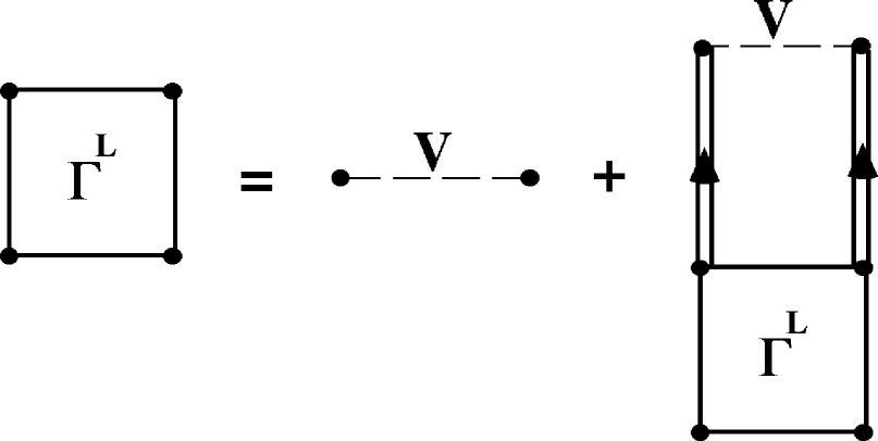
Figure 12: Diagrammatic representation of the ladder equation [Eq. (59)] in the medium. Note that fully dressed propagators are iterated between successive interactions. Only in this diagram the subscript “L” is used to identify the ladder summation.

It is convenient to decompose the effective interaction in two parts as in done in Eq. (59b) which separates the energy-dependent part from the energy-independent NN interaction $V$. Employing this separation, one obtains the nucleon self-energy in the form shown diagrammatically in Fig. 4$a)$ with $U$ discarded and the full vertex function replaced by the corresponding ladder approximation. The diagram with the closed loop corresponds to the energy-independent contribution involving the NN interaction

$$\Sigma_{V}(k)=\int\frac{d^{3}k^{\prime}}{(2\pi)^{3}}\left\langle{\bm{k}}{\bm{k}}^{\prime}\right|V\left|{\bm{k}}{\bm{k}}^{\prime}\right\rangle n(k^{\prime}),$$ (60)

with

$$n(k)=\int_{-\infty}^{\varepsilon_{F}}d\omega\ S_{h}(k,\omega)$$ (61)

representing the correlated momentum distribution. Note that explicit summation over spin and isospin projections have been suppressed and a notation with individual particle momenta ${\bm{k}}$ and ${\bm{k}}^{\prime}$ is used for the two-body interaction in Eq. (60). Both the effective interaction and the self-energy fulfill important dispersion relations which are helpful in devising strategies to achieve a numerically tractable self-consistency procedure. For the energy-dependent part of the effective interaction one has

$$\left\langle{\bm{q}}\right|\Delta\Gamma({\bm{K}},\Omega)\left|{\bm{q}}^{\prime}\right\rangle = \frac{-1}{\pi}\int_{2\varepsilon_{F}}^{\infty}\!\!\!d\Omega^{\prime}\ \frac{\textrm{Im}\ \left\langle{\bm{q}}\right|\Delta\Gamma({\bm{K}},\Omega^{\prime})\left|{\bm{q}}^{\prime}\right\rangle}{\Omega-\Omega^{\prime}+i\eta}+\frac{1}{\pi}\int^{2\varepsilon_{F}}_{-\infty}\!\!\!d\Omega^{\prime}\ \frac{\textrm{Im}\ \left\langle{\bm{q}}\right|\Delta\Gamma({\bm{K}},\Omega^{\prime})\left|{\bm{q}}^{\prime}\right\rangle}{\Omega-\Omega^{\prime}-i\eta}\hskip 17.07182pt$$ (62a)

$$\equiv \left\langle{\bm{q}}\right|\Delta\Gamma_{\downarrow}({\bm{K}},\Omega)\left|{\bm{q}}^{\prime}\right\rangle+\left\langle{\bm{q}}\right|\Delta\Gamma_{\uparrow}({\bm{K}},\Omega)\left|{\bm{q}}^{\prime}\right\rangle.$$ (62b)

The decomposition of the effective interaction into forward and backward-going contributions as exhibited in Eq. (62) is essential to obtain a proper construction of the self-energy [86]. Indeed, using Eqs. (56) and (62a) one obtains the remaining contributions to the self-energy in the following way

$$\Sigma_{\Delta\Gamma}(k,\omega) = \int\frac{d^{3}k^{\prime}}{(2\pi)^{3}}\int_{-\infty}^{\varepsilon_{F}}d\omega^{\prime}\ \left\langle{\bm{k}}{\bm{k}}^{\prime}\right|\Delta\Gamma_{\downarrow}(\omega+\omega^{\prime})\left|{\bm{k}}{\bm{k}}^{\prime}\right\rangle S_{h}(k^{\prime},\omega^{\prime})$$ (63a)

$$- \int\frac{d^{3}k^{\prime}}{(2\pi)^{3}}\int_{\varepsilon_{F}}^{\infty}d\omega^{\prime}\ \left\langle{\bm{k}}{\bm{k}}^{\prime}\right|\Delta\Gamma_{\uparrow}(\omega+\omega^{\prime})\left|{\bm{k}}{\bm{k}}^{\prime}\right\rangle S_{p}(k^{\prime},\omega^{\prime})$$

$$\equiv \Delta\Sigma_{\downarrow}(k,\omega)+\Delta\Sigma_{\uparrow}(k,\omega).$$ (63b)

As for Eq. (60) the notation for the two-body matrix elements of $\Delta\Gamma$ involve individual momenta. The result of Eq. (63) also implies the following dispersion relation for the self-energy

$$\Sigma(k,\omega) = \Sigma_{V}(k)-\frac{1}{\pi}\int_{\varepsilon_{F}}^{\infty}d\omega^{\prime}\frac{\textrm{Im }\ \Sigma(k,\omega^{\prime})}{\omega-\omega^{\prime}+i\eta}+\frac{1}{\pi}\int^{\varepsilon_{F}}_{-\infty}d\omega^{\prime}\frac{\textrm{Im}\ \Sigma(k,\omega)}{\omega-\omega^{\prime}-i\eta}$$ (64a)

$$= \Sigma_{V}(k)+\Delta\Sigma_{\downarrow}(k,\omega)+\Delta\Sigma_{\uparrow}(k,\omega).$$ (64b)

Using this self-energy in the Dyson equation one obtains

$$g(k,\omega) = g^{(0)}(k,\omega)+g^{(0)}(k,\omega)\Sigma(k,\omega)g(k,\omega)$$ (65a)

$$= \frac{\omega-\varepsilon(k)-\textrm{Re}\ \Sigma(k,\omega)+i\textrm{Im}\ \Sigma(k,\omega)}{\left(\omega-\varepsilon(k)-\textrm{Re}\ \Sigma(k,\omega)\right)^{2}+\left(\textrm{Im}\ \Sigma(k,\omega)\right)^{2}},$$ (65b)

where the explicit form of the noninteracting propagator

$$g^{(0)}(k,\omega)=\frac{\theta(k-k_{F})}{\omega-\varepsilon(k)+i\eta}+\frac{\theta(k_{F}-k)}{\omega-\varepsilon(k)-i\eta}$$ (66)

with

$$\varepsilon(k)=\frac{k^{2}}{2m}$$ (67)

is used to obtain the result of Eq. (65b). The diagrammatic version of the Dyson equation is shown in Fig. 1. Although it is now possible to solve the ladder equation with mean-field propagators without an angle-averaging procedure [87, 88], it is necessary for a practical implementation using fully dressed propagators to make this approximation. To obtain the ladder equation in a partial wave basis one therefore proceeds by an angle-averaging procedure for the noninteracting but dressed two-particle propagator

$$g^{II}_{f}({\bm{q}};{\bm{K}},\Omega) = \frac{i}{2\pi}\int d\omega\ g({\bm{K}}/2+{\bm{q}},\Omega/2+\omega)g({\bm{K}}/2-{\bm{q}},\Omega/2-\omega)$$ (68)

$$= \int_{\varepsilon_{F}}^{\infty}d\omega_{1}\int_{\varepsilon_{F}}^{\infty}d\omega_{2}\ \frac{S_{p}({\bm{K}}/2+{\bm{q}},\omega_{1})S_{p}({\bm{K}}/2-{\bm{q}},\omega_{2})}{\Omega-\omega_{1}-\omega_{2}+i\eta}$$

$$- \int_{-\infty}^{\varepsilon_{F}}d\omega_{1}\int_{-\infty}^{\varepsilon_{F}}d\omega_{2}\ \frac{S_{h}({\bm{K}}/2+{\bm{q}},\omega_{1})S_{h}({\bm{K}}/2-{\bm{q}},\omega_{2})}{\Omega-\omega_{1}-\omega_{2}-i\eta}.$$

Eq. (68) shows that the angle-averaging is confined to the numerators. It is therefore possible to consider the imaginary part of $g^{II}_{f}$ for this purpose. For $\Omega>2\varepsilon_{F}$ one has

$$\textrm{Im}\ g^{II}_{f}({\bm{q}};{\bm{K}},\Omega)=-\frac{1}{\pi}\int_{2\varepsilon_{F}}^{\infty}d\omega\ S_{p}({\bm{K}}/2+{\bm{q}},\Omega/2+\omega)\ S_{p}({\bm{K}}/2-{\bm{q}},\Omega/2-\omega)$$ (69)

and for $\Omega<2\varepsilon_{F}$ the corresponding result is given by

$$\textrm{Im}\ g^{II}_{f}({\bm{q}};{\bm{K}},\Omega)=\frac{1}{\pi}\int_{-\infty}^{2\varepsilon_{F}}d\omega\ S_{h}({\bm{K}}/2+{\bm{q}},\Omega/2+\omega)\ S_{h}({\bm{K}}/2-{\bm{q}},\Omega/2-\omega)$$ (70)

The convolution integrals in Eqs. (69) and (70) also provide a practical route to obtain the real part of $g^{II}_{f}$ by means of the following dispersion relation

$$g^{II}_{f}({\bm{q}};{\bm{K}},\Omega)=-\frac{1}{\pi}\int_{2\varepsilon_{F}}^{\infty}d\Omega^{\prime}\ \frac{\textrm{Im}\ g^{II}_{f}({\bm{q}};{\bm{K}},\Omega^{\prime})}{\Omega-\Omega^{\prime}+i\eta}+\frac{1}{\pi}\int_{-\infty}^{2\varepsilon_{F}}d\Omega^{\prime}\ \frac{\textrm{Im}\ g^{II}_{f}({\bm{q}};{\bm{K}},\Omega^{\prime})}{\Omega-\Omega^{\prime}-i\eta}.$$ (71)

The cycle of steps necessary to perform a self-consistent calculation of the sp propagator is now complete. Starting from a reasonable set of spectral functions, the construction of the noninteracting but dressed two-particle propagator first requires the convolution integrals given in Eqs. (69) and (70). In a next step the dispersion integrals in Eq. (71) can be used to obtain the real part of the this propagator. After an angle-averaging procedure the resulting propagator only depends on the absolute values of the relative and total momenta. It is therefore permissible to solve for the ladder equation in a partial wave basis

$$\left\langle q\ell\right|\Gamma^{JST}(K,\Omega)\left|q^{\prime}\ell^{\prime}\right\rangle = \left\langle q\ell\right|V^{JST}\left|q^{\prime}\ell^{\prime}\right\rangle$$

$$+ \sum_{\ell^{\prime\prime}}\int_{0}^{\infty}dp\ p^{2}\left\langle q\ell\right|V^{JST}\left|p\ell^{\prime\prime}\right\rangle g^{II}_{f}(p;K,\Omega)\left\langle p\ell^{\prime\prime}\right|\Gamma^{JST}(K,\Omega)\left|q^{\prime}\ell^{\prime}\right\rangle.$$

According to Eq. (63b) one only needs the diagonal elements of the imaginary part of $\Gamma$ (properly adding the different partial wave contributions) and the original input spectral functions to obtain the imaginary part of the self-energy. The dispersion integrals in Eq. (64) together with Eq. (60) then allow the construction of the complete real part of the self-energy. The solution of the Dyson equation is then straightforward. One finally obtains the new spectral functions from

$$S_{p}(k,\omega)=\frac{-1}{\pi}\frac{\textrm{Im}\ \Sigma(k,\omega)}{\left(\omega-\varepsilon(k)-\textrm{Re}\ \Sigma(k,\omega)\right)^{2}+\left(\textrm{Im}\ \Sigma(k,\omega)\right)^{2}}$$ (73)

for energies above $\varepsilon_{F}$ and from

$$S_{h}(k,\omega)=\frac{1}{\pi}\frac{\textrm{Im}\ \Sigma(k,\omega)}{\left(\omega-\varepsilon(k)-\textrm{Re}\ \Sigma(k,\omega)\right)^{2}+\left(\textrm{Im}\ \Sigma(k,\omega)\right)^{2}}$$ (74)

for energies below $\varepsilon_{F}$. At this point the cycle can be repeated until by some numerical criteria the input sp propagator is sufficiently close to the output sp propagator. One of the most important quantities to emerge from the spectral functions is the energy per particle [26]

$$\frac{E}{A}=\frac{2}{\rho}\int\frac{d^{3}k}{(2\pi)^{3}}\int_{-\infty}^{\varepsilon_{F}}d\omega\ \left(\frac{k^{2}}{2m}+\omega\right)S_{h}(k,\omega),$$ (75)

where $\rho$ is the density both related to the Fermi momentum by

$$\rho=\frac{2k_{F}^{3}}{3\pi^{2}}$$ (76)

and the self-consistent momentum distribution

$$\rho=\frac{2}{\pi^{2}}\int_{0}^{\infty}dkk^{2}\ n(k)$$ (77)

since self-consistency guarantees particle number conservation [29, 30]. One may also separately consider the kinetic energy per particle

$$\frac{T}{A}=\frac{2}{\pi^{2}}\int_{0}^{\infty}dkk^{2}\ \frac{k^{2}}{2m}n(k).$$ (78)

The potential energy can then be obtained by considering the difference between Eqs. (75) and (78). This general outline requires further details related to a suitable numerical implementation. Some of these aspects will be considered in Sec. 4.6 where results for fully self-consistent spectral functions are discussed.

4.2 Spectral functions obtained from mean-field input

The first generation spectral functions were based on the solution of the scattering equation (Eq. (4.1) ) employing mf propagators in the construction of $g^{II}_{f}$ with corresponding $\delta$ function spectral functions. The corresponding result for the self-energy given in Eq. (63) also simplifies and is given by

$$\Sigma_{\Delta\Gamma}(k,\omega) = \int\frac{d^{3}k^{\prime}}{(2\pi)^{3}}\left\langle\bm{k}\bm{k}^{\prime}\right|\Delta\Gamma_{\downarrow}^{(0)}(\omega+\varepsilon(k^{\prime}))\left|\bm{k}\bm{k}^{\prime}\right\rangle\ \theta(k_{F}-k^{\prime})$$ (79)

$$- \int\frac{d^{3}k^{\prime}}{(2\pi)^{3}}\left\langle\bm{k}\bm{k}^{\prime}\right|\Delta\Gamma_{\uparrow}^{(0)}(\omega+\varepsilon(k^{\prime}))\left|\bm{k}\bm{k}^{\prime}\right\rangle\ \theta(k^{\prime}-k_{F}),$$

where a superscript has been attached to $\Gamma$ to identify that it was obtained from a scattering equation with mf propagators. A serious difficulty arises when propagating mf propagators corresponding to a continuous sp spectrum in the ladder equation when a realistic NN interaction is employed [62]. Indeed, so-called pairing instabilities arise in the ${}^{3}S_{1}$-${}^{3}D_{1}$ and ${}^{1}S_{0}$ partial wave channels in certain density regimes [64]. Self-consistency with unperturbed propagators in the ladder equation can be achieved while solving the above difficulties and still maintaining a connection between the sp potential and the full $\Sigma$ by making the following choices [61]: Below $k_{F}$, let $\varepsilon(k)$ be the first moment of $S_{h}(k,\omega)$ with respect to energy (the contribution to the total energy at that momentum) divided by the number of particles in the system with that momentum. One cannot extend this intuitive prescription to $k>k_{F}$ by replacing $S_{h}$ with $S_{p}$ since $S_{p}$ contains a significant fraction of strength up to GeV energies and would result in unrealistically large values for $\varepsilon(k)$ when $k>k_{F}$. Therefore, above $k_{F}$, $S_{p}$ is replaced with the quasiparticle (qp) contribution to $S_{p}$. This is equivalent to setting $\varepsilon(k)$ equal to the qp energy (discussed in more detail below). One then obtains

$$\varepsilon(k)=\frac{\int d\omega\ \omega\ S_{h}(k,\omega)}{\int d\omega\ S_{h}(k,\omega)}\hskip 156.49014ptk<k_{F}$$ (80)

and

$$\varepsilon(k)=\frac{\int d\omega\ \omega\ S_{qp}(k,\omega)}{\int d\omega\ S_{qp}(k,\omega)}=\frac{k^{2}}{2m}+\textrm{Re}\ \Sigma(k,\varepsilon_{qp}(k))\hskip 28.45274ptk>k_{F}.$$ (81)

The above prescription for the $sp$ spectrum requires calculation of the full energy dependence of $\Sigma$ in each iteration step and is therefore more computationally intensive. However, it naturally contains a gap large enough to prevent the pairing instabilities. More details related to this prescription of self-consistency can be found in Ref. [62]. The qp energy alone has no appreciable gap, but near the Fermi momentum there is considerable spreading of hole strength to energies below the qp energy.

Some results from this scheme will be reviewed now to establish a benchmark for the second-generation spectral functions discussed in Sec. 4.6. One characteristic feature of the resulting imaginary part of the self-energy is shown in Fig. 13.

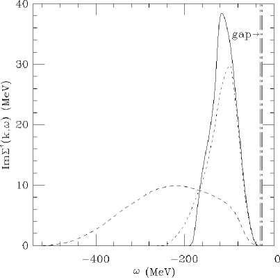
Figure 13: Imaginary part of the self-energy as a function of energy below the gap for three momenta, $k=0.01$ (solid), $0.51$ (dotted), and $2.1~{}\textrm{fm}^{-1}$ (dashed).

Comparing different values of $k$ for these energies below the Fermi energy indicates that Im$\Sigma^{\uparrow}$ becomes weak while its energy range enlarges in a smooth manner as $k$ increases. The energy range for this Im$\Sigma^{\uparrow}$ is determined by using the analysis of Ref. [56]. This analysis shows that for each $k$ there is a minimum energy above which 2h1p states (of mf type) can mix in the self-energy. So momentum conservation and the constraint on the location of 2h1p energies due to their mf character are responsible for the energy range observed in Fig. 13. This wide range of energies will be available to the hole spectral functions discussed below.

For momenta near $k_{F}$ one finds that the energy dependence of $S_{h}$ and $S_{p}$ is dominated by the qp peak characterizing the extent to which noninteracting features are maintained. Each momentum has an associated qp energy which is the solution of

$$\varepsilon_{qp}(k)=\frac{k^{2}}{2m}+\textrm{Re}\Sigma(k,\varepsilon_{qp}(k)).$$ (82)

The spectral function displays a peak at $\varepsilon_{qp}$ because of the vanishing term in the denominator of Eq. (73) or (74). The qp-peak itself is represented by

$$S_{qp}(k,\omega)=\frac{1}{\pi}\frac{Z^{2}(k)\mid W(k)\mid}{(\omega-\varepsilon_{qp}(k))^{2}+(Z(k)W(k))^{2}}$$ (83)

where $W(k)=\textrm{Im}\ \Sigma(k,\varepsilon_{qp}(k))$ and

$$Z(k)=\left\{1-\left(\frac{\partial\textrm{Re}\ \Sigma(k,\omega)}{\partial\omega}\right)_{\omega=\varepsilon_{qp}(k)}\right\}^{-1}$$ (84)

is the strength contained in the peak. These first-generation SCGF calculations show that near $k_{F}$ the qp peak contains around 70% of the total sp strength, while an extra 13% is contained in the background composing the remainder of hole strength. The background is uniformly distributed across several hundred MeV below $\varepsilon_{F}$ corresponding to the range of Im $\Sigma$ but depends significantly on the value of $k$ as shown in Fig. 14. The final 17% of the strength has moved to energies greater than $\varepsilon_{F}$ including a significant high-energy tail in $S_{p}$ discussed momentarily. Farther below $k_{F}$ this picture breaks down as the qp peak melts into the background resulting in hole strength which is spread over a much wider range of energies. To the extent that spectral functions are described by the qp approximation, the excitations in nuclear matter are like those of a Landau Fermi-liquid as illustrated in Fig. 14. This figure contains several hole spectral functions for momenta below the Fermi momentum at $k_{F}=1.36~{}\textrm{fm}^{-1}$.

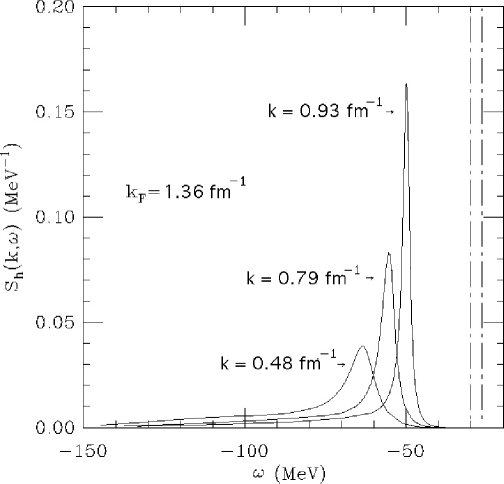
Figure 14: Illustration of the decreasing width of the quasiparticle peak in the spectral function for three momenta below $k_{F}$ given by $k=0.48$, 0.79, and $0.93~{}\textrm{fm}^{-1}$. The vertical lines indicate the position of the gap in the sp spectrum that results from employing Eqs. (80) and (81).

Notice that as $k\rightarrow k_{F}$ this peak becomes extremely sharp due to the vanishing Im$\Sigma$ in Eq. (74). The infinite-lifetime character of such excitations is made possible by the loss of phase-space available to the states in $\Sigma$ near the Fermi energy. This is essentially the same argument used by Landau in more general terms to develop the microscopic foundations of Fermi-liquid theory [89].

In Fig. 15 the particle spectral function is plotted for three different momenta, $k=0.79,~{}1.74,$ and $5.04~{}\textrm{fm}^{-1}$ as a function of energy.

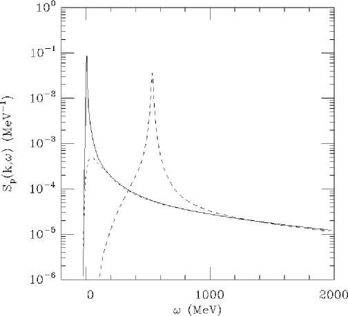
Figure 15: Particle spectral functions at $k=0.79$ (dotted), $1.74$ (solid), $5.04~{}\textrm{fm}^{-1}$ (dashed). All three spectral functions converge to the same tail at high energy.

All momenta below $k_{F}$ have the same high-energy tail as the dotted curve for $k=0.79~{}\textrm{fm}^{-1}$ in Fig. 15. For momenta larger than $k_{F}$ a quasiparticle peak, which broadens with increasing momentum, can be observed on top of the same high-energy tail. The results therefore display a common, essentially momentum independent, high-energy tail. The location of sp strength at high energy simply means that the interaction has sufficiently large matrix elements to compensate energy denominators encountered in the ladder equation. For this particular interaction a significant amount of strength is found at high energy. This result was of course already anticipated a long time ago [90].

A quantitative characterization of the missing $sp$ strength for $k=0.79~{}\textrm{fm}^{-1}$ shows that the integrated strength accounts for 17% of the sp strength. This is in agreement with the sum rule since the integrated hole strength provides 83% of sp strength. The strength in the interval from 100 MeV above the Fermi energy to infinity amounts to 13% with 7% residing above 500 MeV. To understand the influence of the tensor force on this distribution, a calculation of the ladder equation was performed in which the tensor coupling in the ${}^{3}S_{1}$-${}^{3}D_{1}$ coupled channel was switched off. In this case, the integrated sp strength amounts to 10.5% and should be regarded as resulting from pure short-range correlations. In Ref. [61] it is shown that the tensor force moves the additional 6.5% of strength to the first 1000 MeV above the Fermi energy. This is consistent with CBF calculations of the momentum distribution which show depletions of a similar size due to tensor correlations [91].

Figure 16 exhibits the graph of the occupation probability, $n(k)$, or the number of particles in the ground state of the system with sp quantum number $k$.

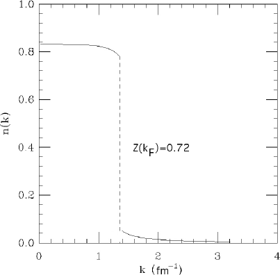
Figure 16: Occupation probability for nuclear matter at equilibrium density obtained by integrating hole spectral functions obtained with mean-field propagators as input.

Near $k=0$, $n(k)$ becomes fairly constant with a value of 0.83. From the discussion of $S_{p}$, roughly $1/3$ of the 17% depletion is due to the effect of tensor correlations in the ladder equation. Another $1/3$ is due the to high-energy tail in $S_{p}$ at energies above 500 MeV. Results from other many-body methods such as Brueckner theory [92, 93] and CBF theory [58] using other realistic interactions give very similar occupation near $k=0$. In Refs. [92] and [93], 0.82 is reported for the Paris potential. Older CBF calculations for the Urbana $v_{14}$ interaction give 0.87 whereas more recent CBF results [91] give 0.83. All these calculations for different interactions using different methods give a strikingly similar result for $n(0)$. This was encouraging since it implies that non-relativistic many-body calculations are under control in the region where one would like to compare to finite nuclei.

In contrast to $n(0)$, the occupation at $k_{F}$ varies significantly between methods. This variability is most easily expressed in terms of the discontinuity in $n(k)$ at $k_{F}$, $Z(k_{F})\equiv n(k^{-}_{F})-n(k^{+}_{F})$. For the result shown in Fig. 16, $Z(k_{F})=0.72$ and for the CBF calculation $Z(k_{F})=0.70$. However, for the Paris interaction, $Z(k_{F})=0.35$ and $Z(k_{F})=0.47$ has been obtained in Refs. [92] and [93], respectively. The extra depletion in $n(k)$ as $k\rightarrow k_{F}$ arises from the enhanced ability of the sp state to couple to low lying 2p1h excitations as its energy approaches the 2p1h states. Also, the discontinuity depends on the level at which pairing correlations are included in the calculation. In the case of a paired system $Z(k_{F})$ would be zero.

4.3 Spectral functions for $\Lambda$-hyperons obtained from mean-field input

Hypernuclei, especially those with one $\Lambda$ hyperon, have been studied for a long time [94, 95]. When a $\Lambda$ hyperon is placed in a nucleus or nuclear matter it will interact with the nucleons in its environment. As a result of these strong interactions, the $\Lambda$ becomes correlated with nucleons in the medium. The study of the properties of the $\Lambda$ hyperon in an environment of nucleons aims to answer a number of fundamental questions related to the properties of strange particles in the nuclear medium. Considerable attention has been given to the potential energy the $\Lambda$ experiences in the nucleus and the corresponding single-particle (sp) energies. From this experimental work it becomes clear that the $\Lambda$ hyperon is less strongly bound to nucleons than either a proton or a neutron. Such sp properties have been studied theoretically for finite nuclei by several groups [96] - [99]. The general conclusion from the experimental work is that the $\Lambda$ hyperon experiences a potential well in the nucleus that has the familiar Woods-Saxon shape with a depth of about 30 MeV for a wide range of heavier nuclei. Global sp properties of the $\Lambda$ hyperon can be studied in nuclear matter. Results of such calculations have also been reported by several groups [100] - [106].

The correlations of the $\Lambda$ hyperon in nuclear matter have typically been studied at the level of its average binding or sp energy. Full propagation of the $\Lambda$ including the determination of its complex self-energy has not been reported sofar. In view of the relevance of the properties of a strange particle in a nuclear system, it seems timely to study the properties of a $\Lambda$ hyperon when it is embedded in such a nuclear system. As in the case of NN interactions, typical hyperon-nucleon (YN) interactions  [107] - [112] incorporate substantial repulsion at short distance. As discussed above, the consequences of this strong interaction can be accounted for in the framework of the Green’s function formalism by including the proper treatment of these short-range correlations (SRC) in the form of ladder-diagram summation for the hyperon-nucleon interaction in the medium ($G$ matrix). The effects on the dynamical single-particle properties of the $\Lambda$ can then be explored by evaluating the complex self-energy of the $\Lambda$ in nuclear matter. The solution of the Dyson equation for the $\Lambda$ then yields again information on the net binding of the $\Lambda$ in nuclear matter, but also determines the distribution of spectral strength for its addition to the nuclear-matter ground state as a result of SRC. Such a spectral function for a $\Lambda$ hyperon is shown in Fig. 17.

Figure 17: Spectral function for a $\Lambda$ with $k$ = 100 MeV/c [84, 113]. The vertical dashed line indicates the position of a delta-function spectral distribution for the limiting case of a free particle. Because of the 30 MeV binding for a $\Lambda$ in nuclear matter, it is convenient to shift the horizontal axis by 40 MeV for plotting on a log scale.

The addition of a strange test particle opens the door for quantitative comparisons with spectral functions obtained for nucleons discussed in the previous section. The weaker YN interaction is expected to result in similar but less extreme modifications to the spectral distribution. However, the presence of the $\Lambda$ hyperon also requires consideration of its heavier sibling, the isospin one $\Sigma$ hyperon. The two hyperons have a small enough mass difference that a coupled-channel problem must be solved. In the case of the $\Lambda$ propagator some qualitative changes occur in comparison with the case of the nucleon propagator. The result corresponding to Eq. (56) now becomes

$$g_{\Lambda}(k;\omega)=\int_{\varepsilon_{T}^{\Lambda}}^{\infty}d{\omega}^{\prime}\frac{S_{\Lambda}(k;{\omega}^{\prime})}{\omega-{\omega}^{\prime}+i\eta}.$$ (85)

Since no Fermi surface for $\Lambda$ hyperons is considered here, it is not possible to remove a $\Lambda$ from the NM ground state. As a result, the propagator only contains the probability amplitude for adding a $\Lambda$ particle with momentum $k$ at an energy ${\omega}^{\prime}$. The energy threshold at which it becomes possible to add a $\Lambda$ to the NM ground state is denoted by $\varepsilon_{T}^{\Lambda}$. One expects this energy to be accessible only for a $\Lambda$ at rest ($k=0$). If the $\Lambda$ were added to a free Fermi gas NM ground state and would not be correlated otherwise, this threshold energy would simple be the kinetic energy of a $\Lambda$ with zero momentum and would therefore correspond to zero energy. Based on previous work by other groups [102, 104] one expects the actual value of the threshold energy at normal NM density to be around $-30\ \textrm{MeV}$ indicating the substantial attraction a $\Lambda$ experiences in NM. Since the $\Lambda$ can only propagate as a particle, the spectral strength above the threshold energy must integrate to 1. This condition on the $\Lambda$ spectral function is given by

$$\int_{\varepsilon_{T}^{\Lambda}}^{\infty}d{\omega}^{\prime}S_{\Lambda}(k;{\omega}^{\prime})=n_{p,\Lambda}(k)=1.$$ (86)

This result is quite different from the corresponding nuclear case where one has to consider the strength in the particle domain to supplement the contribution given by Eq. (61). As in the case of nucleons one can obtain the spectral function from the imaginary part of the propagator

$$S_{\Lambda}(k;\omega)=-\frac{1}{\pi}\textrm{Im}~{}g_{\Lambda}(k;\omega)\hskip 42.67912pt\omega>\varepsilon_{T}^{\Lambda}.$$ (87)

The sp spectral function as shown for example in Fig. 17 involves the overlap between the simple physical state given by

$$a_{\Lambda\bm{k}}^{{\dagger}}\left|\Psi_{0}\right\rangle$$ (88)

and the complicated eigenstate

$$\left|{}^{\Lambda}\Psi(E)\right\rangle.$$ (89)

which includes all interactions between the $\Lambda$ and the nuclear medium. The extent to which there is overlap illustrates how well the $\Lambda$ sp state survives intact in the medium. For the case of no interactions between the $\Lambda$ and the nucleons, the overlap is perfect, since the state of Eq. (88) is an eigenstate in this situation. This is evidenced by the $\delta$ function spectral distribution appropriate for a free particle, as indicated by a dashed line at the kinetic energy in Fig. 17. Interactions between the $\Lambda$ and nucleons are responsible for the transition from the simple $\delta$ function structure to the more complex distribution of sp strength realized in NM. The mechanism behind the spreading of sp strength can be understood as the mixing of a sp state at a given energy with 2p1h states which span a continuum of energies.

Although the sp state is no longer an eigenstate of the many-body Hamiltonian, its quantum numbers are still conserved by the interaction. The total strength associated with the original sp state, though fragmented, is fixed. This is reflected in the sum rule of Eq. (86). Details of the strength distribution are determined by the density of 2p1h states which increases with energy and the strength with which the interaction couples these states to the unperturbed sp state. This information is summarized in the imaginary part of the self-energy, shown for example in Fig. 18. Note that the decomposition in partial wave contributions emphasizes the dominance of the ${}^{3}S_{1}$ channel.

Figure 18: Imaginary part of the $\Lambda$ self-energy for $k$ = 100 MeV/c. The broken curves represent contributions to the overall self-energy from the ${}^{3}S_{1}$ (dash) and ${}^{1}S_{0}$ (dot) partial wave channels.

A nuclear matter calculation for nucleons similar to this one [61] yields a particle spectral function shown in Fig. 19, for a momentum just above $k_{F}$.

Figure 19: Nucleon particle spectral function (solid) for $k=316$ MeV/c with lambda spectral function (dashed) at $k=60$ MeV/c for comparison.

The $Z$-factor obtained from this calculation is $Z_{N}(k_{F})=0.72$, which is substantially reduced compared to $Z_{\Lambda}(0)=0.87$ for a similar $\Lambda$ qp state. These two momentum values are compared because each qp sits at the lowest possible excitation energy for a qp in the respective systems. In Ref. [61], this depletion of the qp strength is explained in terms of couplings to 2h1p states, which moves approximately 10% of the sp strength to energies below $\varepsilon_{F}$, and coupling to 2p1h states, which distributes another 18% to higher energies in the particle domain. The corresponding fraction of sp strength in the particle domain is 13% for the $\Lambda$, compared to 18% for nucleons. Turning off the $\Lambda N$-$\Sigma N$ coupling in the Nijmegen soft core (NSC) potential reveals [110] that tensor effects are responsible for almost half of the reduction in the $\Lambda$ qp strength consistent with the nucleon case discussed in Sec. 4.2. A value of $Z_{\Lambda}(k_{F}^{\Lambda})=0.94$ is obtained when coupling to $\Sigma N$ states is cut off.

Away from the qp peak, at high-energy, the size and structure of the spectral function is primarily determined by two factors. The density of 2p1h states increases like $\omega^{1/2}$ at high energy. This growth in spectral strength with energy is moderated by the strength of the coupling to these high-energy states. A $\Lambda$ with a reasonably low momentum couples to a nucleon hole state only with a low relative momentum. The high-energy $\Lambda N$ two-particle states couple most strongly to high relative momentum and the strength of the potential matrix elements between these two states depends on the short-range characteristics of the two-body interaction. A harder core allows a stronger coupling between states and correspondingly more spectral strength at high energy. The fact that structure in the high-energy region of the spectral function is primarily determined by the short-range behavior of the two-body interaction should be tempered by the knowledge that the short-range part of baryon-baryon interactions are poorly known. Typical potentials are designed, within whatever model, to fit only low-energy experimental data which does little to constrain the details of the repulsive core. This situation can be taken in two ways. On the one hand, the high-energy tail of the spectral function is just as uncertain in detail as the core of the interaction from which it is derived. On the other hand, it is also just as experimentally inaccessible and any observable which can be related to the detail of the tail in the spectral strength distribution could be used to gain insight into the behavior of the bare two-body interaction at short-range. In Fig. 20 the similarities of the tail of the spectral strength for different momenta is illustrated.

Figure 20: Spectral function for three values of $k_{\Lambda}$ show the $k$-independence of the high energy tail for $k$ = 10 MeV/c (solid curve), 110 MeV/c (dashed), and 210 MeV/c (dash-dot).

We note that this common feature of the strength is identical to the case of nucleons illustrated in Fig. 15. The only difference is in the distribution of the strength which reflects the hardness of the underlying interaction. In conclusion, one may state that the properties of a $\Lambda$ hyperon in nuclear matter are qualitatively quite similar to those of a nucleon. The physical consequences of the underlying interactions with their strong repulsive cores are also quite similar. Naturally, there are quantitative differences which indicate that a nucleon is somewhat stronger correlated with the nuclear medium than a $\Lambda$. Nevertheless, a common high-energy tail for the sp strength and a similar role for the tensor force in reducing the qp strength also emphasize the common features of these strongly interacting particles in the medium.

4.4 Healing properties of nuclear wave functions

The conceptual understanding of strongly interacting nucleons yielding a mf shell-model (Fermi-gas) picture has relied heavily on the concept of the healing of the relative wave function to the noninteracting one as discussed in Refs. [19, 20]. Experimental evidence based on the (e,e^′p) reaction [15] has demonstrated that nucleon sp motion must be understood in terms of Landau’s quasiparticle description [89]. In turn, this requires a substantial modification of the simple shell-model or Fermi-gas picture. The conventional Bethe-Goldstone propagator used to determine the effective interaction in the medium leads to the healing property of the relative two-nucleon wave function and takes proper care of short-range correlations [19, 20]. However, the corresponding effective interaction is not sufficient to generate a nucleon self-energy which realistically describes the sp strength distribution below the Fermi energy both in nuclear matter and finite nuclei. Inclusion of additional terms involving hole-hole propagation as in a Galitski-Feynman propagator is essential to achieve a realistic spectral function [55, 114]. The main problem with the Bethe-Goldstone propagator is that it generates no self-energy diagrams which couple to 2h1p states. As a result, the experimentally observed fragmentation of the sp strength can not be described in this approach. Inclusion of hole-hole propagation in the ladder equation solves this problem of describing the fragmentation of the sp strength below the Fermi energy. However, this inclusion destroys the healing property of the relative function since it produces a nonvanishing phase shift in the relative wave function for energies below twice the Fermi energy [115] when mf propagators are employed. The resolution of this puzzle requires the consideration of the consequences of the dressing of the nucleons for the description of the scattering process in the medium [85]. In order to clarify this issue it is therefore necessary to delve in to the details of this scattering process and elucidate the essential differences with the corresponding process involving free or mf particles.

For the purpose of the present discussion it is sufficient to consider the two-time two-particle propagator as given by Eq. (57). The main objective of this development is to study the consequences of propagating dressed particles for the description of the scattering process. All subsequent discussion will be based on the solution of a Lippmann-Schwinger-type scattering equation for the effective interaction which is equivalent to summing the ladder diagrams for a particular choice of noninteracting two-body propagator and two-body interaction. In order to clarify the difference between the conventional discussion of scattering in free space and the one necessary for the medium, it will be useful to cast the description completely in the language of the two-body propagator. While this is certainly not necessary for the scattering of free particles, it will provide a simple way to clarify the changes that are required to extend the description to dressed particles in the medium.

It is important to realize that the usual results from scattering theory are obtained in the coordinate representation. The relevant double Fourier transform of the two-particle propagator in Eq. (57) is given by

$$g^{II}(\bm{r},\bm{r}^{\prime};\Omega)~{}=~{}\frac{1}{(2\pi)^{3}}\int\!\!d^{3}q\ \int\!\!d^{3}q^{\prime}\ e^{i\bm{q}\cdot\bm{r}}g^{II}(\bm{q},\bm{q}^{\prime};\Omega)\ e^{-i\bm{q}^{\prime}\cdot\bm{r}^{\prime}},$$ (90)

where without loss of generality we consider the case that the total momentum $K$ is zero. The transform of the noninteracting propagator only involves one integration due to the presence of the $\delta$ function in Eq. (58)

$$g^{II}_{f}(\bm{r},\bm{r}^{\prime};\Omega)=\frac{1}{(2\pi)^{3}}\int\!\!d^{3}q\ \int\!\!d^{3}q^{\prime}\ e^{i\bm{q}\cdot\bm{r}}g^{II}_{f}(\bm{q},\bm{q}^{\prime};\Omega)\ e^{-i\bm{q}^{\prime}\cdot\bm{r}^{\prime}}=\frac{1}{(2\pi)^{3}}\int\!\!d^{3}q\ e^{i\bm{q}\cdot(\bm{r}-\bm{r}^{\prime})}g^{II}_{f}(\bm{q};\Omega).$$ (91)

The result for Eq. (57) can then be transformed to yield

$$g^{II}(\bm{r},\bm{r}^{\prime};\Omega) = g^{II}_{f}(\bm{r},\bm{r}^{\prime};\Omega)+\int\!\!d^{3}r_{1}\ \int\!\!d^{3}r_{2}\ g^{II}_{f}(\bm{r},\bm{r}_{1};\Omega)\ \langle\bm{r}_{1}|V|\bm{r}_{2}\rangle\ g^{II}(\bm{r}_{2},\bm{r}^{\prime};\Omega)$$ (92a)

$$= g^{II}_{f}(\bm{r},\bm{r}^{\prime};\Omega)+\int\!\!d^{3}r_{1}\ \int\!\!d^{3}r_{2}\ g^{II}_{f}(\bm{r},\bm{r}_{1};\Omega)\ \langle\bm{r}_{1}|\Gamma(\Omega)|\bm{r}_{2}\rangle\ g^{II}_{f}(\bm{r}_{2},\bm{r}^{\prime};\Omega).$$ (92b)

Employing these equations one can arrive at an asymptotic analysis and resulting definition of the cross section which is equivalent to a standard analysis involving the equation for the wave function in the case of scattering in free space or mf particles in the medium. Before this result is developed, it is useful to summarize the propagator equations in the partial-wave representation. These allow the introduction of the phase shift which contains the relevant information to obtain the asymptotic propagator or wave function in this representation.

A partial wave decomposition of the two-body propagator in Eq. (57) yields the corresponding integral equation and the relation between the propagator and the vertex function

$$g^{II}_{JST}(q\ell,q^{\prime}\ell^{\prime};\Omega) = \frac{\delta(q-q^{\prime})}{q^{2}}\delta_{\ell,\ell^{\prime}}g^{II}_{f}(q;\Omega)+g^{II}_{f}(q;\Omega)\sum_{\ell^{\prime\prime}}\int\!\!dpp^{2}\langle q\ell|V^{JST}|p\ell^{\prime\prime}\rangle g^{II}_{JST}(p\ell^{\prime\prime},q^{\prime}\ell^{\prime};\Omega)\hskip 25.6073pt$$ (93a)

$$= \frac{\delta(q-q^{\prime})}{q^{2}}\delta_{\ell,\ell^{\prime}}g^{II}_{f}(q;\Omega)+g^{II}_{f}(q;\Omega)\langle q\ell|\Gamma^{JST}(\Omega)|q^{\prime}\ell^{\prime}\rangle g^{II}_{f}(k^{\prime};,\Omega),$$ (93b)

where the vertex function or effective interaction $\Gamma$ can be obtained from the numerical solution of the ladder equation in a partial-wave momentum representation as given in Eq. (4.1). The energy $\Omega$ is conserved and must be viewed as a variable upon which the propagator depends (it also depends on the total momentum in the case of the medium). The noninteracting propagator is again denoted by $g^{II}_{f}$ and may include the dressing of the individual particles when the scattering takes place in matter.

The coordinate space version of Eq. (93) is obtained by a double Fourier-Bessel transform

$$g^{II}_{JST}(r\ell,r^{\prime}\ell^{\prime};\Omega)=\frac{2}{\pi}\int_{0}^{\infty}\!\!\!dq~{}q^{2}\int_{0}^{\infty}\!\!\!dq^{\prime}~{}q^{\prime}{}^{2}~{}j_{\ell}(qr)j_{\ell^{\prime}}(q^{\prime}r^{\prime})\ g^{II}_{JST}(q\ell,q^{\prime}\ell^{\prime};\Omega).$$ (94)

The corresponding result for the noninteracting part of the propagator, represented by the first term in Eq. (93), reduces to one integral on account of the $\delta$ function which conserves relative momentum

$$g^{II}_{f,\ell}(r,r^{\prime};\Omega)=\frac{2}{\pi}\int_{0}^{\infty}\!\!\!dq~{}q^{2}~{}j_{\ell}(qr)j_{\ell}(qr^{\prime})g^{II}_{f}(q;\Omega).$$ (95)

The Fourier-Bessel transform of Eq. (93) then has the following form

$$g^{II}_{JST}(r\ell,r^{\prime}\ell^{\prime};\Omega)\!\!\! = \!\!\delta_{\ell,\ell^{\prime}}g^{II}_{f,\ell}(r,r^{\prime};\Omega)+\!\!\sum_{\ell^{\prime\prime}}\int_{0}^{\infty}\!\!\!\!\int_{0}^{\infty}\!\!\!\!dr_{1}r_{1}^{2}\ dr_{2}r_{2}^{2}g^{II}_{f,\ell}(r,r_{1};\Omega)\langle r_{1}\ell|V^{JST}|r_{2}\ell^{\prime\prime}\rangle g^{II}_{JST}(r_{2}\ell^{\prime\prime},r^{\prime}\ell^{\prime};\Omega)\hskip 8.5359pt$$ (96)

$$= \!\!\delta_{\ell,\ell^{\prime}}g^{II}_{f,\ell}(r,r^{\prime};\Omega)+\!\!\int_{0}^{\infty}\!\!\!\!\int_{0}^{\infty}\!\!\!dr_{1}r_{1}^{2}dr_{2}r_{2}^{2}\ g^{II}_{f,\ell}(r,r_{1};\Omega)\langle r_{1}\ell|\Gamma^{JST}(\Omega)|r_{2}\ell^{\prime}\rangle g^{II}_{f,\ell^{\prime}}(r_{2},r^{\prime};\Omega).$$

When the bare two-body interaction $V$ is local in the relative coordinate, only one integral in the first equality remains. The second equality can be used to study the asymptotic behavior of the propagator outside the range of the interaction.

The subsequent discussion for the scattering of dressed particles in the medium requires the consideration of the two-body propagator in the medium. For this reason it is advantageous to collect the conventional results for scattering in free space using this language. In the case of free particles the noninteracting propagator in momentum space is given by

$$g^{II}_{f}(q;\Omega)=\frac{1}{\Omega-\hbar^{2}q^{2}/m+i\eta}.$$ (97)

Defining the on-shell momentum by

$$\Omega=\frac{\hbar^{2}q_{0}^{2}}{m},$$ (98)

one can perform the relevant Fourier-Bessel transform of the noninteracting propagator in Eq. (95) analytically (see e.g. [116]) with the well-known result

$$g^{II}_{f,\ell}(r,r^{\prime};q_{0})=-iq_{0}\frac{m}{\hbar^{2}}j_{\ell}(q_{0}r_{<})h_{\ell}(q_{0}r_{>}).$$ (99)

The coordinate argument in the spherical Hankel function must be the larger of $r$ and $r^{\prime}$ and is denoted by $r_{>}$ while the argument of the spherical Bessel function is the smaller and denoted by $r_{<}$. For the current analysis it will be assumed that the interaction has a finite range, $\langle r|V|r^{\prime}\rangle=0$ for $r,r^{\prime}$ larger than some $r_{0}$. Substituting Eq. (99) in the second part of Eq. (96) in the case of an uncoupled channel for $r^{\prime}>r$ and $r^{\prime}>r_{0}$ yields

$$g^{II}_{\ell JST}(r,r^{\prime};q_{0}) = -iq_{0}\frac{m}{\hbar^{2}}j_{\ell}(q_{0}r)h_{\ell}(q_{0}r^{\prime})$$ (100)

$$+ \int_{0}^{\infty}\!\!\!\!\int_{0}^{\infty}\!\!\!\!dr_{1}r_{1}^{2}\ dr_{2}r_{2}^{2}~{}g^{II}_{f,\ell}(r,r_{1};q_{0})\langle r_{1}|T^{JST}_{\ell}(q_{0})|r_{2}\rangle\left(-iq_{0}\frac{m}{\hbar^{2}}\right)j_{\ell}(q_{0}r_{2})h_{\ell}(q_{0}r^{\prime})$$

$$= -iq_{0}\frac{m}{\hbar^{2}}\psi^{JST}_{\ell}(r;q_{0})h_{\ell}(q_{0}r^{\prime}),$$

where

$$\psi^{JST}_{\ell}(r;q_{0})=j_{\ell}(q_{0}r)+\int_{0}^{\infty}\!\!\!\!\int_{0}^{\infty}dr_{1}r_{1}^{2}\ dr_{2}r_{2}^{2}~{}g^{II}_{f,\ell}(r,r_{1};q_{0})\langle r_{1}|T^{JST}_{\ell}(q_{0})|r_{2}\rangle j_{\ell}(q_{0}r_{2}),$$ (101)

and the conventional notation $T$ instead of $\Gamma$ has been introduced together with the replacement of $\Omega$ by $q_{0}$. This result demonstrates that under the given conditions the propagator separates as a product of a function of $r$ and a function of $r^{\prime}$. This result can be substituted into the first part of Eq. (96) to obtain the relevant integral equation for the wave function $\psi$ (under the condition that $r^{\prime}>r_{0}$)

$$\psi^{JST}_{\ell}(r;q_{0})=j_{\ell}(q_{0}r)+\int_{0}^{\infty}\!\!\!\!\int_{0}^{\infty}\!\!\!\!dr_{1}r_{1}^{2}\ dr_{2}r_{2}^{2}~{}g^{II}_{f,\ell}(r,r_{1};q_{0})\langle r_{1}|V^{JST}_{\ell}|r_{2}\rangle\psi^{JST}_{\ell}(r_{2};q_{0}),$$ (102)

which can be found in standard textbooks (see e.g. [116] for the case of a local potential). It is derived here to demonstrate the relation between the propagator and the wave function since for the case of dressed particles one has to start with the formulation in terms of propagators.

The asymptotic analysis of the propagator can be performed by using Eq. (99) in Eq. (96) under the assumption that the propagator will be considered for $r<r^{\prime}$ while both these coordinates are larger than $r_{0}$, the range of the interaction. Values of $r_{1}$ and $r_{2}$ in Eq. (96) larger than $r_{0}$ yield no contributions to the integral. As a result, the effective interaction, $T$, has a range similar to the one of the bare interaction $V$. Using the relation between spherical Bessel and Hankel functions

$$j_{\ell}(\rho)=\frac{1}{2}\left(h_{\ell}(\rho)+h^{*}_{\ell}(\rho)\right),$$ (103)

one obtains the asymptotic behavior of the propagator for the case of an uncoupled partial wave channel from the second part of Eq. (96) in the following form

$$g^{II}_{\ell,JST}(r,r^{\prime};q_{0})\rightarrow -i\left(\frac{m}{2\hbar^{2}}\right)q_{0}h_{\ell}(q_{0}r^{\prime})\bigg{\{}h_{\ell}^{*}(q_{0}r)+h_{\ell}(q_{0}r)\times$$

$$\left[1-2i\frac{m}{\hbar^{2}}q_{0}\int_{0}^{\infty}\!\!\!\!\int_{0}^{\infty}\!\!\!\!dr_{1}~{}r_{1}^{2}~{}dr_{2}~{}r_{2}^{2}~{}\langle r_{1}|T^{JST}_{\ell}(q_{0})|r_{2}\rangle j_{\ell}(q_{0}r_{1})j_{\ell}(q_{0}r_{2})\right]\bigg{\}}$$

$$= -i\frac{m}{2\hbar^{2}}q_{0}h_{\ell}(q_{0}r^{\prime})\left\{h_{\ell}^{*}(q_{0}r)+h_{\ell}(q_{0}r)\left[1-2\pi i\left(\frac{mq_{0}}{2\hbar^{2}}\right)\langle q_{0}|T^{JST}_{\ell}(q_{0})|q_{0}\rangle\right]\right\}.$$

In the last step of Eq. (LABEL:eq:asymni) one can return to the on-shell matrix element of the $T$-matrix in momentum space which completely determines the outcome of the scattering process. The term in square brackets corresponds to the $S$-matrix element in terms of which one can define the phase shift

$$\langle q_{0}|S^{JST}_{\ell}(q_{0})|q_{0}\rangle=\left[1-2\pi i\left(\frac{mq_{0}}{2\hbar^{2}}\right)\langle q_{0}|T^{JST}_{\ell}(q_{0})|q_{0}\rangle\right]\equiv e^{2i\delta_{\ell}^{JST}}.$$ (105)

This result can be represented by

$$\tan\delta^{JST}_{\ell}=\frac{\textrm{Im}\ \langle q_{0}|T^{JST}_{\ell}(q_{0})|q_{0}\rangle}{\textrm{Re}\ \langle q_{0}|T^{JST}_{\ell}(q_{0})|q_{0}\rangle},$$ (106)

which explicitly shows that a nonzero imaginary part of the effective interaction is required to obtain a nonvanishing phase shift. In turn, this imaginary part of the interaction only appears for energies where the noninteracting propagator has a nonvanishing imaginary part. For the scattering of free particles this corresponds to all positive energies. By substituting the explicit form of the spherical Hankel functions for $\ell=0$ in Eq. (LABEL:eq:asymni) one can construct the asymptotic propagator for the ${}^{1}S_{0}$ channel explicitly

$$g^{II}_{\ell,{}^{1}S_{0}}(r,r^{\prime};q_{0})\rightarrow-i\frac{m}{2q_{0}\hbar^{2}}\frac{1}{rr^{\prime}}e^{i(q_{0}r^{\prime}+\delta_{{}^{1}S_{0}})}\sin(q_{0}r+\delta_{{}^{1}S_{0}}).$$ (107)

The standard result for the asymptotic wave function is contained in this equation and the imaginary part of Eq. (107) is simply the product of these wave functions as a function of $r$ and $r^{\prime}$, respectively.

To obtain the relation between the cross section and the propagator it is necessary to return to Eq. (92) and perform the Fourier transform of the noninteracting propagator (Eq. (97)) in Eq. (91). This Fourier transform is given by the well-known result (again replacing the energy $\Omega$ by the on-shell momentum $q_{0}$)

$$g^{II}_{f}(\bm{r},\bm{r}^{\prime};q_{0})=-\frac{m}{4\pi\hbar^{2}}\frac{e^{iq_{0}|\bm{r}-\bm{r}^{\prime}|}}{|\bm{r}-\bm{r}^{\prime}|}.$$ (108)

A similar procedure as used for the asymptotic analysis in the partial wave basis can be employed to obtain the corresponding result for Eq. (92). Whereas in the former analysis the separable form of the noninteracting propagator in Eq. (99) is valid without constraint on $r$ and $r^{\prime}$, this is not the case here since Eq. (108) only becomes separable in the case $r^{\prime}\gg r$ or vice versa. In the former case one can write Eq. (108) as

$$g^{II}_{f}(\bm{r},\bm{r}^{\prime};q_{0})\rightarrow-\frac{m}{4\pi\hbar^{2}}\frac{e^{iq_{0}r^{\prime}}}{r^{\prime}}e^{-iq_{0}\hat{\bm{r}}^{\prime}\cdot\bm{r}}.$$ (109)

Substituting this result in the second part of Eq. (92) for both $r^{\prime}\gg r$ and $r^{\prime}\gg r_{2}$ demonstrates that $g^{II}$ is separable and can be written as

$$g^{II}({\mbox{\boldmath$r$}},{\mbox{\boldmath$r$}}^{\prime};q_{0})=-\frac{m}{4\pi\hbar^{2}}\frac{e^{iq_{0}r^{\prime}}}{r^{\prime}}\psi(\bm{r};q_{0})$$ (110)

in the asymptotic domain. By substituting this result in turn in Eq. (92) one obtains the standard integral equation for the wave function and the appropriate formulation for the asymptotic wave function to obtain the scattering amplitude

$$\psi(\bm{r};q_{0}) = e^{-iq_{0}\hat{\bm{r}}^{\prime}\cdot\bm{r}}+\int\!\!\!d^{3}r_{1}\int\!\!\!d^{3}r_{2}~{}g^{II}_{f}(\bm{r},\bm{r}_{1};q_{0})\langle\bm{r}_{1}|V|\bm{r}_{2}\rangle\psi(\bm{r}_{2};q_{0})$$ (111)

$$= e^{-iq_{0}\hat{\bm{r}}^{\prime}\cdot\bm{r}}+\int\!\!\!d^{3}r_{1}\int\!\!\!d^{3}r_{2}~{}g^{II}_{f}(\bm{r},\bm{r}_{1};q_{0})\langle\bm{r}_{1}|T(q_{0})|\bm{r}_{2}\rangle e^{-iq_{0}\hat{\bm{r}}^{\prime}\cdot\bm{r}_{2}}.$$

One may identify the origin of the motion in the direction of the negative $z$-axis, meaning that $\hat{\bm{r}}^{\prime}$ points in that direction, so that $\bm{q}\equiv-q_{0}\hat{\bm{r}}^{\prime}$ points into the positive $z$-direction. If one assumes that $r$ is also much larger than the range of the potential, and, therefore much larger than any contributing value of $r_{1}$, one can use Eq. (109) again in the second part of Eq. (111) to identify the coefficient multiplying the outgoing spherical wave $e^{iq_{0}r}/r$ as the scattering amplitude (while double Fourier transforming the $T$-matrix element back to momentum space)

$$f_{q_{0}}(\theta,\phi)=-\frac{2m\pi^{2}}{\hbar^{2}}\langle\bm{q}^{\prime}|T(q_{0})|\bm{q}\rangle,$$ (112)

where $\theta,\phi$ denote the angles associated with the direction of $\hat{\bm{r}}$ and $\bm{q}^{\prime}\equiv q_{0}\hat{\bm{r}}$ corresponds to the momentum of the detected motion in the direction $\hat{\bm{r}}$ with the same absolute value $q_{0}$ as the initial state. The differential cross section for the direction $(\theta,\phi)$ is then simply the square of the scattering amplitude as given by Eq. (112)

$$\frac{d\sigma}{d\Omega}=\left|f_{q_{0}}(\theta,\phi)\right|^{2}.$$ (113)

The present formulation is closely tailored to the conventional experimental situation where a collimated beam propagates along the $z$-axis characterized by a given energy or momentum toward a target situated at the origin. Detection then takes place in a particular direction away from the origin characterized by angles $\theta$ and $\phi$. The only difference is that the present formulation is appropriate for the corresponding center-of-mass system ($K=0$).

To obtain the phase shifts and cross sections for particles propagating in the medium with mf sp energies one can proceed in similar fashion. A useful reference is the work of Bishop et al. [115] where the introduction of the phase shift for the case of hole-hole propagation is discussed. While some details are different in this case, the main points of the previous analysis remain valid when both particle-particle and hole-hole propagation is taken into account. The corresponding mf propagator in the medium, also known as the Galitski-Feynman propagator, is given in momentum space by

$$g^{II}_{mf}(q;\Omega)=\frac{\theta(q-k_{F})}{\Omega-2\varepsilon(q)+i\eta}-\frac{\theta(k_{F}-q)}{\Omega-2\varepsilon(q)-i\eta},$$ (114)

where, again, the case of zero center-of-mass momentum is considered. The sp energy $\varepsilon(q)$ can deviate from the simple kinetic energy spectrum and therefore yield a different relation between the energy $\Omega$ and the on-shell momentum $q_{0}$

$$\Omega\equiv 2\varepsilon(q_{0}),$$ (115)

nevertheless the uniqueness of $q_{0}$ for a given energy is still preserved. Although one can no longer evaluate the noninteracting propagator in coordinate space completely analytically from Eq. (95), the separability of the propagator is maintained for the contribution of the pole term as in Eq. (99) (with a different constant prefactor), while the remaining term vanishes asymptotically for $r$ sufficiently different from $r^{\prime}$. A discussion of a similar result for the Fourier transform of the mf propagator given in Eq. (114) can be found in Ref. [117] for the Bethe-Goldstone propagator. As a result, one preserves the integral equations for the wave function either in a partial wave basis as in Eq. (101) or for the wave function in coordinate space as in Eq. (111) in the case of mf propagators. The only difference with the free scattering case involves the use of the mf equivalents of the noninteracting propagators in coordinate space in Eqs. (102) and (111). This result is due to the uniqueness of the on-shell momentum at a given energy which guarantees that the noninteracting wave function is a plane wave or spherical Bessel function (in a partial wave basis). One can therefore proceed with a similar asymptotic analysis as for free particles yielding a corresponding definition of the phase shifts as in Eq. (105) in terms of the on-shell scattering matrix. The result of Eq. (106) also remains valid in this case. The presence of a nonvanishing phase shift is therefore continued to be linked to the nonvanishing of the imaginary part of the noninteracting propagator. In the case of mf scattering the corresponding energy domain resides above $2\varepsilon(q=0)$ which corresponds to the lowest energy of two hole states.

These modest modifications of the quantities that characterize the scattering process as compared to the case of free-particle scattering, are related to the continued one-to-one relation of the energy with a unique relative momentum for which the noninteracting propagator has an imaginary part. This on-shell momentum emerges as the momentum that characterizes the plane wave (or spherical Bessel function) function describing the relative motion. The plane-wave character of the wave function allows for a conventional interpretation of the scattering process as in free space.

Since the correlated wave function does not heal to the uncorrelated one when hole-hole propagation is included, the usual discussion of healing must be indeed be modified as indicated above. The standard interpretation of the validity of the shell model is couched in terms of the healing of the relative wave function to the noninteracting one. This interpretation was put forward in Ref. [19] and is based on the use of the Bethe-Goldstone propagator in describing the effective interaction. Since this propagator excludes the propagation of two holes in Eq. (114), the correction to the relative wave function in Eq. (102) due to the strong interaction potential heals within a characteristic healing distance to the spherical Bessel function provided that the energy is less than twice the Fermi energy. In scattering language this simply states that there is no phase shift for energies less than $2\varepsilon_{F}$ when the Bethe-Goldstone propagator is employed since no corresponding imaginary part of the propagator exists [20].

An apparent contradiction then arises with this interpretation when one realizes that it is not permitted to neglect the propagation of the hole-hole term in Eq. (114) since it is essential for the understanding of the fragmentation of the sp strength below the Fermi energy [57]. Inclusion of hole-hole propagation yields a nonvanishing phase shift below $2\epsilon_{F}$ [115] which is at odds with the healing interpretation of the relative wave function. On the other hand this contribution to the effective interaction is responsible for the presence of an imaginary part of the nucleon self-energy which is required in order to describe the experimental situation in nuclei as obtained from the (e,e^′p) reaction [15]. Evidently it is not possible to propagate mf nucleons which can generate a realistic sp strength distribution, and, at the same time, obtain the healing of the relative wave function to the noninteracting one which supposedly underlies the success of the mf picture.

While recent (e,e^′p) experiments have sharpened the range of the validity of the sp picture in terms of the more appropriate Landau quasiparticle description [89] which is adequately described by microscopic theory [55, 114], the paradox at the level of the relative wave function remains. A clue to the solution of this puzzle is provided by noting the inconsistency of the description of the sp strength in terms of a realistic spectral function and the construction of the effective interaction by means of a mf propagator. Clearly if the dressing effect of the nucleon is substantial and experiment [15] indicates it is, then one is forced to consider the construction of the effective interaction in terms of dressed nucleons. The consequences of this extension for the description of the scattering process in matter and the resolution of the healing paradox will be taken up in the following.

The propagation of dressed nucleons requires a different treatment of the description of the scattering process. The main ingredient for this change is the form of the noninteracting propagator which is given in the medium by Eq. (68) and for sp momenta $\bm{k}$ and $\bm{k}^{\prime}$ reads

$$g^{II}_{f}(\bm{k},\bm{k}^{\prime};\Omega)=\int_{\varepsilon_{F}}^{\infty}\!\!\!d\omega\int_{\varepsilon_{F}}^{\infty}\!\!\!d\omega^{\prime}\frac{S_{p}(\bm{k},\omega)S_{p}(\bm{k}^{\prime},\omega^{\prime})}{\Omega-\omega-\omega^{\prime}+i\eta}-\int_{-\infty}^{\varepsilon_{F}}\!\!\!d\omega\int_{-\infty}^{\varepsilon_{F}}\!\!\!d\omega^{\prime}\frac{S_{h}(\bm{k},\omega)S_{h}(\bm{k}^{\prime},\omega^{\prime})}{\Omega-\omega-\omega^{\prime}-i\eta}.$$ (116)

The particle and hole spectral functions, $S_{p}$ and $S_{h}$ respectively, describe the distribution of the sp strength for a given momentum over the energy. These distributions are continuous and have sizable peaks either above or below the Fermi energy, corresponding to a momentum state above or below $k_{F}$, at the so-called quasiparticle energy. For $k_{F}=1.36~{}\textrm{fm}^{-1}$, corresponding to normal density, the strength contained in the peak for momenta close to $k_{F}$ is typically only 70% [61, 59]. From the rest of the strength we refer for more details to the discussion in Sec. 4.2.

It should be noted that the noninteracting propagator in Eq. (116) becomes the familiar mf Galitski-Feynman propagator (see Eq. (114)) when mf spectral functions are inserted which are characterized by a $\delta$ function peak of strength 1 at a sp energy either above the Fermi energy ($k>k_{F}$) or below ($k<k_{F}$). The difference between the Galitski-Feynman propagator and the dressed propagator is qualitatively different for the imaginary part and quantitatively for the real part. In Fig. 21 both the real and imaginary part of the dressed propagator (Eq. (116)) are shown as a function of the relative momentum for zero total momentum while the energy corresponds to an on-shell momentum $q_{0}=0.5~{}\textrm{fm}^{-1}$ in the Galitski-Feynman case using a sp spectrum from Ref. [62]. In the latter case the imaginary part of the propagator contains a $\delta$ function only at a single momentum corresponding to 0.5 $\textrm{fm}^{-1}$. It arises on account of the vanishing of the denominator in the hole-hole term at the on-shell momentum. The full curve in Fig. 21 corresponds to the imaginary part of the dressed propagator shown here as a function of momentum up to $k_{F}$.

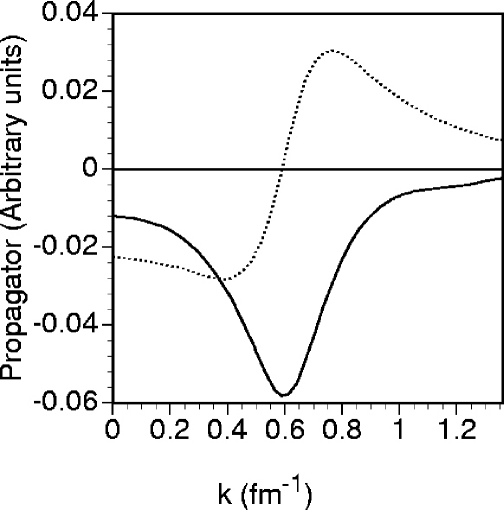
Figure 21: Real (dotted) and imaginary part (full line) of the noninteracting propagator of dressed particles at an energy corresponding to an on-shell momentum of 0.5 $\textrm{fm}^{-1}$ for the mf propagator.

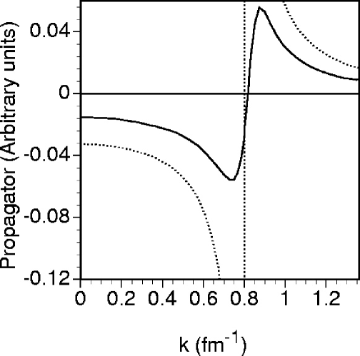
Figure 22: Comparison of the real part of the mf (dotted) and dressed (full line) propagator at an on-shell momentum of 0.8 $\textrm{fm}^{-1}$ indicated by the vertical dotted line.

There is a substantial spreading in the imaginary part containing even small high-momentum components (not shown in Fig. 21). This spreading is a critical feature which completely alters the conventional picture of the scattering process. In Fig. 22 the real part of the dressed and mf propagator are compared for momenta below $k_{F}$ for an energy corresponding to an on-shell momentum of 0.8 $\textrm{fm}^{-1}$. The dotted line corresponds to the mf propagator and also indicates the pole present at 0.8 $\textrm{fm}^{-1}$. The dressed propagator shows a less dramatic momentum dependence and is in general substantially reduced from the mf propagator except for high momenta where both coincide.

In order to perform the analysis of the scattering process it will be illustrative to use an analytical approximation to the noninteracting propagator of dressed particles (Eq. (116)) which contains the essential new features. In addition, only the case of zero total momentum of the propagating pair will be considered in the following. As a result, the noninteracting propagator contains equal and opposite momenta for the two particles (holes). Since the spectral functions do not depend on the direction of the momentum one can rewrite Eq. (116) for the present purposes as

$$g^{II}_{f}(k,\Omega)=\int_{\varepsilon_{F}}^{\infty}\!\!\!d\omega\int_{\varepsilon_{F}}^{\infty}\!\!\!d\omega^{\prime}\frac{S_{p}(k,\omega)S_{p}(k,\omega^{\prime})}{\Omega-\omega-\omega^{\prime}+i\eta}-\int_{-\infty}^{\varepsilon_{F}}\!\!\!d\omega\int_{-\infty}^{\varepsilon_{F}}\!\!\ d\omega^{\prime}\frac{S_{h}(k,\omega)S_{h}(k,\omega^{\prime})}{\Omega-\omega-\omega^{\prime}-i\eta}.$$ (117)

The momentum $k$ not only corresponds to the absolute value of the sp momenta but also represents the relative momentum for the case of zero total momentum.

Introducing a two-body self-energy term for purely practical reasons, one can attempt to write this noninteracting propagator as

$$g^{II}_{f}(k,\Omega)=\frac{\pm 1}{\Omega-\Sigma^{II}(k,\Omega)},$$ (118)

where the sign is determined by whether the energy $\Omega$ is above (+) or below (-) 2$\varepsilon_{F}$. By assuming that this ad hoc self-energy $\Sigma^{II}$ has a slowly varying imaginary part as a function of the relative momentum $k$ one can expand the self-energy at the momentum $k_{0}$ for which

$$\Omega\equiv\textrm{Re}\ \Sigma^{II}(k_{0},\Omega).$$ (119)

Noting that the expansion is in the square of the momentum, one obtains a complex pole approximation (CPA) to the propagator by only keeping the real and imaginary part of $\Sigma^{II}$ at $k_{0}^{2}$ and the first derivative of the real part. The resulting propagator has the form

$$g^{II}_{f,CPA}(k,\Omega)=\frac{m}{\hbar^{2}}\frac{\pm c}{k_{0}^{2}-k^{2}\pm i\gamma},$$ (120)

where the constant $c$ is obtained from

$$c=\frac{\hbar^{2}}{m}\left(\left.\frac{\partial{\rm Re}\Sigma^{II}}{\partial k^{2}}\right|_{k_{0}^{2}}\right)^{-1}$$ (121)

and $\gamma$ from

$$\gamma=\left|{\rm Im}\Sigma^{II}(k_{0},\Omega)\right|\left(\left.\frac{\partial{\rm Re}\Sigma^{II}}{\partial k^{2}}\right|_{k_{0}^{2}}\right)^{-1}.$$ (122)

Typical values of $c$ at low energies correspond to 0.5 whereas it rises slowly to 1 for higher energies. This feature is closely related to the pattern of the distribution of the sp strength. The quasiparticle pole strength at $k_{F}$ = 1.36 $\textrm{fm}^{-1}$ is about 0.7 (see Sec. 4.2) so for a two-particle propagator close to these energies a factor of $(0.7)^{2}$ is expected. For higher momenta the strength in the peak grows back to 1 yielding a propagator which is more of the mf or even free-particle kind. It is also apparent that this factor of about 0.5 can be identified from Fig. 22. It should be noted that the CPA is obtained after first numerically calculating the noninteracting propagator of the dressed particles. In Fig. 23 the quality of this CPA to the propagator can be judged by comparing it to the numerically calculated result for the imaginary part of the propagator at an energy below 2$\varepsilon_{F}$.

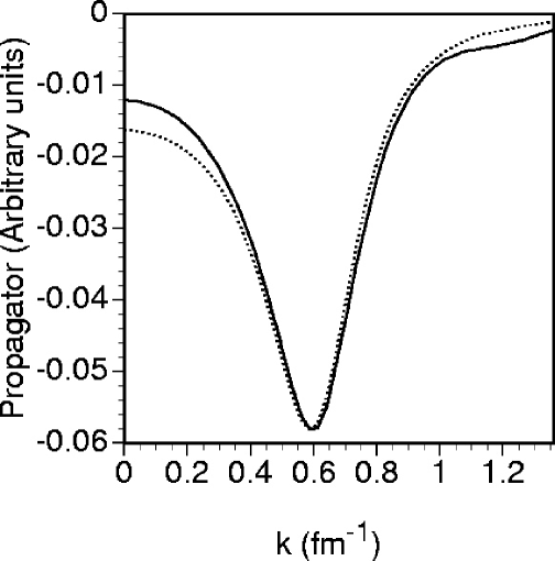
Figure 23: Comparison for the imaginary part of the noninteracting propagator of dressed nucleons between the complete (numerical) result given by the full line and the simple CPA given by the dotted line for momenta below $k_{F}$.

The CPA result for the propagator cannot be used to solve any of the integral equations for the effective interaction for example since it is only a good approximation to the noninteracting propagator close to the peak of the imaginary part. The full solution also requires an accurate representation of the high-momentum components of the propagator in order to properly include the effect of short-range correlations in the interaction or wave function. The CPA result does provide a reasonable representation of the long-range part of the propagator and therefore can be profitably used to discuss the asymptotic analysis of the scattering process. Indeed, using the CPA to the dressed propagator one can repeat the steps involved in the Fourier-Bessel transform leading to Eq. (99). For free or mf particles the integral in Eq. (95) yields the product of a spherical Bessel function and one of the spherical Hankel functions with as argument the real on-shell momentum $k_{0}$ (see Eqs. (98) and (115)). This on-shell momentum is real since the corresponding noninteracting propagators (Eqs. (97) and (114)) can only have a vanishing denominator for a real momentum. Since Eq. (95) can be calculated by a contour integral for Eqs. (97), (114) (at least for the long-range part), as well as for Eq. (120), it is clear that the presence of a nonvanishing imaginary part for the pole of Eq. (120), due to a the nonvanishing of $\gamma$, will lead to a complex on-shell momentum which will be denoted by $\kappa_{0}$. Using the CPA (Eq. (120)) for $\Omega<2\epsilon_{F}$ one obtains from Eq. (95)

$$g^{II}_{\ell,CPA}(r,r^{\prime};\Omega)=-ic\frac{m}{\hbar^{2}}\kappa_{0}j_{\ell}(\kappa_{0}r_{<})h_{\ell}^{*}(\kappa_{0}r_{>}).$$ (123)

The momentum argument of the spherical Bessel and Hankel functions, $\kappa_{0}$, is now complex, its real and imaginary part, $\kappa_{0}^{R}$ and $\kappa_{0}^{I}$, respectively, are easily obtained from $k_{0}$ and $\gamma$ (see Eqs. (119) and (122)) by determining the zeros of the denominator of Eq. (120). Eq. (123) contains the Hankel function $h_{\ell}^{*}$ due to the different boundary condition associated with hole-hole propagation for energies below $2\epsilon_{F}$. This leads to a pole in the upper half of the complex $k$-plane in contrast to the case of particle-particle or free-particle scattering. As a result, $\kappa_{0}^{I}$ is negative for $\Omega<2\epsilon_{F}$ and its magnitude can become as large as 0.2 to 0.3 $\textrm{fm}^{-1}$. The resulting propagator for $\ell=0$ can be written as (for $r<r^{\prime}$)

$$g^{II}_{\ell=0,CPA}(r,r^{\prime};\Omega)=\frac{-icm}{2\hbar^{2}(\kappa_{0}^{R}+i\kappa_{0}^{I})}\left(\frac{e^{i\kappa_{0}^{R}r}e^{-\kappa_{0}^{I}r}}{r}-\frac{e^{-i\kappa_{0}^{R}r}e^{\kappa_{0}^{I}r}}{r}\right)\frac{e^{-i\kappa_{0}^{R}r^{\prime}}e^{\kappa_{0}^{I}r^{\prime}}}{r^{\prime}}.$$ (124)

A comparison between this analytical result and the numerical Fourier-Bessel transform of the dressed noninteracting propagator which it approximates, is very successful in the domain where the propagator has its maximum as shown in Fig. 24. This is also true for the real part. This demonstrates that the propagator for dressed particles is radically different from the noninteracting or mf one (see Eq. (99)) due to presence of damping terms related to the nonzero value of $\kappa_{0}^{I}$. As noted before, there is no longer a unique on-shell momentum. Indeed, the complex pole at $\kappa_{0}$ in the CPA propagator is just a simple (and approximate) representation of this feature. As a consequence, the relative wave function of the dressed particles contains a spread in momentum states. This, in turn, must yield a localization of the corresponding wave function in coordinate space. This is exhibited in the propagator Eq. (124) which represents the probability amplitude for removing a pair with relative distance $r^{\prime}$ and adding the pair after propagation at $r$ (without interaction between the pair included yet). This amplitude peaks at $r=r^{\prime}$ (see Fig. 24) and is exponentially damped with the decay constant $|\kappa_{0}^{I}|$.

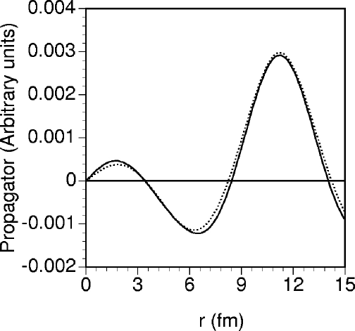
Figure 24: Comparison between the analytical approximation and the complete numerical result for the dressed noninteracting propagator in coordinate space. Shown is the imaginary part for an energy below 2$\varepsilon_{F}$ for the CPA propagator (dotted line) and the complete result (full line). The corresponding propagators in momentum space are shown in Fig. 23.

This feature has interesting physical consequences since it means that if the separation distance between the scatterers is too large there is little probability that they will actually interact because this requires a small relative distance. Indeed, taking $r^{\prime}$ to much larger values than in Fig. 24 yields a negligible contribution to the noninteracting propagator near small $r$ where the interaction will act to modify the wave function. Clearly this effect is governed by the size of $\kappa_{0}^{I}$ the imaginary part of the pole of the CPA. It should be noted that this value will only approach zero when the scattering energy approaches 2$\varepsilon_{F}$. Just as in the case of the sp motion, this means that the noninteracting wave function will tend to a plane wave again only in this limit. The corresponding result for Fig. 24 then yields a simple sine wave characterized by $\kappa_{0}^{R}$ which approaches $k_{F}$. For all other energies damping does occur sufficiently rapidly to warrant the following observation: since only the part of the wave which returns from the scattering can be affected and this part always decreases with increasing $r$, only that part of the noninteracting wave can be influenced by the scattering which is exponentially damped in $r$. This is illustrated in Fig. 25 where a numerical decomposition of the propagator is presented in terms of the incoming and outgoing wave.

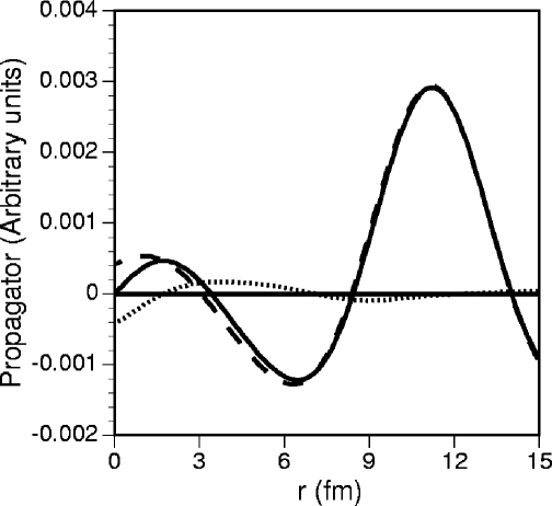
Figure 25: Decomposition of the numerical propagator in coordinate space into in- (dashed) and outgoing wave (dotted line). Also shown is the sum of both contributions (full line).

For values of $r^{\prime}$ outside the range of the interaction as in Fig. 25 this implies that even a substantial modification of the outgoing wave will hardly affect the total propagator and the wave function must automatically heal, according to the equivaqlent value of $\kappa_{0}^{I}$ in CPA approximation, to the noninteracting one.

The above observations allow for the resolution of the paradox related to the healing properties of wave functions in the medium. This property has been considered the physical justification of the mf-like properties observed in nuclei in the presence of strong short-range interactions. There is overwhelming experimental evidence [15] that sp motion in nuclei must be described in terms of dressed nucleons with substantial fragmentation of the strength. The original discussion of the healing properties of the relative wave function of particles in the medium [19] used a Bethe-Goldstone propagator involving mf nucleons to arrive at the healing property of the relative wave function. The present discussion explores the consequences of scattering dressed particles and demonstrates that this dressing of nucleons automatically leads to a localization of the relative wave functions in coordinate space. The results for the CPA propagator analysis indicates that even with sizable phase shifts the localization of the wave function leads to the desired healing property of the wave function since the part of the wave function affected by the scattering event is exponentially damped. Also for the complete numerical propagator the same features are observed. Even in the presence of strong interaction processes the resulting picture of the nuclear medium is a tranquil one in which the dressed particles no longer remember their scattering event beyond some finite distance and their wave functions heal to the corresponding noninteracting ones. This appears to be a satisfactory picture of a correlated medium in which particles do not carry the information of their interaction indefinitely around unlike a description of scattering using a mf Galitski-Feynman propagator.

4.5 In-medium cross sections and phase shifts

For various reasons the study of the interaction between nucleons in the nuclear medium has retained a considerable amount of interest over the years. Of particular interest is the exploration of the “in-medium” interaction in the context of transport-theory descriptions of heavy-ion reactions [118]. Typical analyses simulate the dynamics of a heavy-ion reaction on the basis of kinetic equations like the Boltzmann-Uehling-Uhlenbeck (BUU) equation [119]. An essential ingredient in these BUU calculations is the nucleon-nucleon cross section in the medium. Attempts to include medium-modified cross sections in such calculations have been described in Ref. [120]. Calculations of the cross section between nucleons in nuclear matter have been reported in Refs. [121] - [130]. Some recent issues that have emerged from this work include the enhancement of the cross section at finite temperature due to the vicinity of a pairing instability [127], the sensitivity of the cross section to the choice of the single-particle (sp) spectrum at zero temperature [128], the density and energy dependence [129], and temperature dependence of the cross sections [130].

All results obtained in Refs. [121] -[130] have been generated under the assumption that the sp motion of the nucleon in the medium is that of a mean-field (mf) particle. Under this assumption the scattering process in the medium takes place between nucleons which at most have a sp spectrum different from free space but are otherwise unaffected by the presence of other nucleons except for the Pauli principle related to a mf Fermi gas. This assumption has been contradicted unequivocally in recent years for finite nuclei by the careful analysis of the (e,e^′p) reaction. It is therefore fair to say that both on the basis of experimental results as well as theoretical calculations for nuclear matter, it is prudent to consider the sp dressing of the nucleons in matter and the effect this has on the scattering process. One of the consequences of employing dressed particles is the localization of the two-body propagator in coordinate space as discussed in Sec. 4.4, severely limiting the range of the propagation for most energies. This feature is due to the presence, at a given energy, of a range of momenta which determine the relative wave function of the propagating particles. While for mf particles a unique (on-shell) momentum characterizes the relative wave function which therefore corresponds to a plane wave (or spherical wave), the presence of different momentum components implies that the determination of phase shifts and cross sections requires some kind of folding procedure over these momenta in the case of dressed particles. In Ref. [85] a set of expressions have been introduced to characterize the scattering event of dressed particles involving such a folding procedure. Results for phase shifts and cross sections obtained from these expressions can therefore be compared with the corresponding results propagating free and mf particles using the Reid soft core potential [60].

As proposed in Ref. [85] and followed up in Ref. [67] this folding of the effective interaction takes the following form for the $S$-matrix element in the case of coupled channels

$$S^{JST}_{\ell,\ell^{\prime}}(\Omega)=1+2i\int_{0}^{\infty}dk~{}k^{2}~{}{\rm Im}\left\{g^{II}_{f}(k;\Omega)\right\}\langle k\ell|\Gamma^{JST}(\Omega)|k\ell^{\prime}\rangle.$$ (125)

This result reduces to the conventional results for free or mf particles. In the case of coupled channels Eq. (125) can be used to follow the procedure to obtain phase shifts by diagonalization of the $S$-matrix. For an uncoupled channel, the matrix element in Eq. (125) directly yields the phase shift in the form

$$S^{JST}_{\ell,\ell}(\Omega)=1+2i\int_{0}^{\infty}dk~{}k^{2}~{}{\rm Im}\left\{g^{II}_{f}(k;\Omega)\right\}\langle k\ell|\Gamma^{JST}|k\ell\rangle\equiv e^{2i\delta^{JST}_{\ell}}.$$ (126)

A consequence of the present approximation is that the phase shifts $\delta^{JST}_{\ell}$ remain real [85]. As a result, the phase shifts can be fruitfully compared with results for mf or free particles. Equation (125) is exact for noninteracting or mf particles and for dressed particles includes the physically reasonable expectation that the distribution over the momenta as contained in the imaginary part of the propagator will feature in determining the scattering process. An example of such a distribution was shown in Figs. 21 and 22. While this approximation does not make sense at large distance scales as discussed in the previous section, it provides, locally, a very reasonable generalization of the phase shift. The corresponding “short-distance” approximation to the scattering amplitude yields the following result [85]

$$f^{S}_{m_{s}^{\prime}m_{s}}(\theta,\phi) = 4\pi\sum_{\ell\ell^{\prime}J}\sum_{mm^{\prime}M}i^{\ell^{\prime}}(-i)^{\ell}Y_{\ell m_{\ell}}(\hat{\bm{r}})Y^{*}_{\ell^{\prime}m_{\ell}^{\prime}}(\hat{\bm{z}})(\ell m_{\ell}~{}Sm_{s}|JM)(\ell^{\prime}m^{\prime}_{\ell}~{}Sm^{\prime}_{s}|JM)$$ (127)

$$\int_{0}^{\infty}dk~{}k~{}{\rm Im}\left\{g^{II}_{f}(k;\Omega)\right\}\langle k(\ell S)J|\Gamma(\Omega)|k(\ell^{\prime}S)J\rangle,$$

where a coupling to total spin $S$ and projections $m_{s},m^{\prime}_{s}$ for initial and final spin states has been included together with the usual decomposition in partial waves. For the total cross section (in the neutron-proton case) one obtains

$$\sigma_{tot}=\pi\sum_{S\ell\ell^{\prime}J}(2J+1)\left|\int_{o}^{\infty}dk~{}k~{}{\rm Im}\left\{g^{II}_{f}(k;\Omega)\right\}\langle k(\ell S)J|\Gamma(\Omega)|k(\ell^{\prime}S)J\rangle\right|^{2}.$$ (128)

Eq. (128) demonstrates that a sensible cross section will be obtained in the case of dressed particles at all energies for which a nonvanishing imaginary part of the propagator exists. For two particles deep in the Fermi sea, for example, Eq. (128) avoids the divergence associated with the $k_{0}^{-2}$ term in the corresponding expression for free or mf particles. The formulation of the cross section in terms of Eq. (128) provides a reasonable way to assess the strength of the interaction between dressed particles in the medium in terms of the square of the relevant transition matrix element ($\Gamma$) multiplied by an appropriate measure of the density of states represented by the imaginary part of the noninteracting propagator.

The main results for the phase shifts for some of the more important partial wave channels are summarized in Fig. 26. A comparison is made between phase shifts for free particles (solid line), mf particles at $k_{F}=1.36~{}{\rm fm}^{-1}$ (dashed line), and dressed particles (short-dashed line) at the same density for the ${}^{1}S_{0}$, ${}^{3}S_{1}$, ${}^{3}P_{1}$, and ${}^{3}D_{1}$ channels (corresponding to the different panels in Fig. 26) as a function of the on-shell momentum.

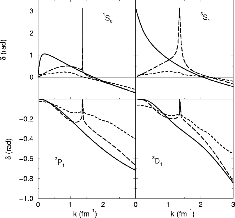
Figure 26: Comparison of phase shifts for free particles (solid), mf particles (dashed), and dressed particles (short-dashed lines) for different partial waves. The density of the medium corresponds to $k_{F}=1.36~{}{\rm fm}^{-1}$.

In general one finds that the dressed phase shifts suggest weaker interactions since in essentially all cases they are either less repulsive or less attractive than the mf result. By studying the individual contributions of the real and imaginary part of the effective interaction one may gain more insight into this issue (see below). For the two $S$-wave channels the most striking feature of the dressed phase shift is the disappearance of the pairing signature for the ${}^{1}S_{0}$ channel and the enormous reduction of the signal in the ${}^{3}S_{1}$ case. While the dressed ${}^{1}S_{0}$ phase shift is essentially zero at $k_{F}$, it is still clearly attractive at this momentum for the ${}^{3}S_{1}$ channel. The actual calculation of the phase shift for this channel displays a slight kink close to $k_{F}$ suggesting that the phase shift may actually rise very rapidly to $\pi$ very close to $k_{F}$. This implies a tremendous reduction in the strength of the pairing correlations in this coupled channel as compared to a mf treatment. Gaps of the order of 10 MeV have been obtained for this channel in Refs. [64, 131, 132]. Clearly, the dressing of the nucleons has a strong influence on pairing. While one would expect to obtain a gap using dressed nucleons based on the attractive effective interaction at the Fermi surface, its magnitude is drastically reduced as suggested by the phase shift calculation shown in Fig. 26. This latter feature has recently been confirmed in Ref. [68]. The main ingredient in this reduction is the decrease in the density of states at $2\epsilon_{F}$ when dressed nucleons are propagated. This reduction is essentially the square of the strength of the quasiparticle pole at $k_{F}$ leading to a reduction factor of about 0.5. Since pairing correlations are particularly sensitive to this density of states, it is not surprising that the strength of the pairing is substantially diminished when dressing is taken into account. It is also noteworthy that one observes a smaller negative phase shift for both $S$-waves at higher energy as compared to the mf result. A similar conclusion may be drawn by inspecting the phase shifts for the ${}^{3}P_{1}$ and ${}^{3}D_{1}$ channel in the bottom panels of Fig. 26. Also for these partial waves which represent repulsive effective interactions, one observes a reduction of the magnitude of the phase shift when dressing is considered. It is also important to note that in the case of mf propagation the results in Fig. 26 show that the corresponding results tend to those of free particles at high energy, whereas this is not the case for dressed particles. This latter result indicates that the effect of the dressing extends to a large energy domain. This observation is not too surprising since the spreading of the sp strength due to short-range and tensor correlations takes place in a very large energy domain [61, 59, 62] and is quite different from a local (in energy) spreading of the strength as would be obtained by a complex quasiparticle energy.

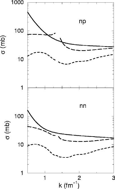
Figure 27: Total neutron-proton (top) and neutron-neutron (bottom panel) cross sections for free (solid), mf (dashed), and dressed particles (short-dashed line) as a function of the on-shell momentum.

The results for the phase shifts obtained for dressed particles lead to the expectation that the corresponding total cross sections are substantially reduced compared to the mf results. The results for neutron-proton (np) and neutron-neutron (nn) total cross sections displayed in Fig. 27 confirm this expectation. Results have been obtained for free (solid), mf (dashed), and dressed particles (short-dashed line) by including all partial wave channels of the Reid potential with $J\leq 2$.

Results for mf particles were generated with a realistic sp energy spectrum and are similar to the corresponding results obtained e.g. in Ref. [128]. The effect of the pairing correlations on the cross sections yields a cusp-like behavior around $k_{F}$ reminiscent of the enhancement of the cross sections obtained by the Rostock group at finite temperature [120, 127]. As the phase shifts for mf particles suggest, the corresponding cross sections in the medium become essentially identical to the one in free space at high energy. Both for the np and nn total cross sections the effect of dressing the nucleons is quite dramatic leading to a substantial reduction of the total cross section at all energies. Indeed, on average a cross section of only about 10 mb is obtained. While this may seem a small number, it should be kept in mind that this by no means implies that the effective interaction in the medium has become insignificant [67]. In addition, one should recall that the concept of asymptotic flux in the medium representing preserved information of a scattering event deep in the medium is not a realistic consideration when the dressing of the nucleons is significant [85], as it is at $k_{F}=1.36~{}{\rm fm}^{-1}$. The main ingredient representing the dressing is the two-particle density of states, its reduction for dressed particles is to a large extent responsible for the reduction of the cross section. In this respect it should be noted that the results of Ref. [127] also show a substantial reduction of the total cross section at high energy with increasing temperature. This result implies that with increasing temperature which also means a larger depletion of the Fermi sea due to thermal excitations, one obtains a reduction of the total cross section similar to the one obtained here at zero temperature when the dressing of the particles is incorporated (and therefore the depletion of the Fermi sea due to correlations is included). While no results are shown in Fig. 27 below 0.5 ${\rm fm}^{-1}$ in order to avoid the large value of the total cross sections for free particles, it should be noted that the cross sections for dressed particles smoothly go to zero when expression (128) is used at lower energies. This expression avoids the problem associated with the expression for free or mf particles which would yield an infinite cross section for the on-shell momentum going to zero. In addition, the latter expression does not yield a cross section for energies that do not yield a solution for the on-shell momentum, i.e. for energies deep in the hole-hole continuum.

A related quantity to the two-body interaction is the two-body propagator given by Eq. (93) in momentum space and Eq. (94) in coordinate space. Since a Lehmann representation exists for this two-particle propagator, it is possible to define a spectral density for this quantity either in momentum or coordinate space. We will consider here

$$S^{II}_{JST}(r\ell,r^{\prime}\ell^{\prime};\Omega)=-\frac{1}{\pi}g^{II}_{JST}(r\ell,r^{\prime}\ell^{\prime};\Omega)$$ (129)

which represents the removal or addition amplitude for a pair of particle (for zero total momentum) depending on whether the energy $\Omega$ is below or above $2\varepsilon_{F}$, respectively. In Fig. 28 this quantity is plotted for $r=r^{\prime}$ in the case of the ${}^{1}S_{0}$ partial wave for an energy corresponding to $-100$ MeV. This diagonal form of Eq. (129) corresponds to the two-particle spectral function in this chosen representation.

Figure 28: Two-nucleon spectral function for the ${}^{1}S_{0}$ channel in nuclear matter for zero total momentum and a removal energy corresponding to $-100$ MeV.

The curves in this figure correspond to the full propagator (labeled $S^{II}$), the contribution of the first term from Eq. (93) representing two dressed but noninteracting nucleons ($S^{II}_{free}$), and the contribution of the second term of Eq. (93) representing the vertex function $\Gamma$ ($S^{II}_{I}$). In addition, the result for two mf particles is shown by the curve labeled $S^{II}_{0}$. Notice that $S^{II}_{free}$ has a large positive value at the origin and $S^{II}_{I}$ has a large negative value at the origin. There is a precise cancellation which is illustrated in Fig. 28. This cancellation is of course associated with the effect of the short-range core of the Reid interaction which suppresses the relative wave function at these disctances. Integrating Eq. (129) over the allowed two-particle removal energies yields the corresponding contribution to the two-particle density matrix

$$\rho^{II}(r\ell,r^{\prime}\ell^{\prime};JST)=\int_{-\infty}^{2\epsilon_{F}}d\Omega\ S^{II}_{JST}(r\ell,r^{\prime}\ell^{\prime};\Omega)$$ (130)

This quantity also characterizes the behavior at short-range for a chosen partial wave and can be compared to the corresponding quantity using dressed but noninteracting propagators. It is attractive to cast this comparison in the form of the ratio

$$C(r)=\frac{\rho^{II}(r\ell,r\ell;JST)}{\rho^{II}_{free}(r\ell,r\ell;JST)}.$$ (131)

In Fig. 29 we plot the correlation function calculated for ${}^{1}S_{0}$ nucleons with center of mass momentum zero.

Figure 29: Correlation function for ${}^{1}S_{0}$ nucleons with total momentum zero.

Note that this correlation function shows the characteristic depression at $r=0$ and an enhancement somewhat above $r=1$ fm. This correlation function has been employed in the analysis of two-proton removal experiments as discussed in Sec. 5.7. In Ref. [133] a related study has been reported for the probability for the removal of pairs with the actual properties of the deuteron yielding information about the deuteron distribution in nuclear matter.

4.6 Results for self-consistent Green’s functions in Nuclear Matter

The solution to the scheme outlined in Sec. 4.1 has been studied by different groups. Aspects of self-consistency have been treated in Refs. [69] - [79]. Complete self-consistency has been implemented for a realistic interaction in terms of a discrete representation of the propagator in Ref. [76]. A representation of the spectral functions on a momentum and energy grid was made self-consistent in Re. [77] for a separable version of the Paris potential. Both of these strategies work better when softer interactions are used. Indeed, it appears that yet another method is required to deal with interactions like the Reid potential [60]. The main reasons for potential problems is the need to consider a very large energy domain since the peaks in the imaginary part of the self-energy and effective interaction occur around 10 GeV [61, 62] for a potential like Reid’s. This feature puts stringent demands on the sizes of grids to describe the spectral strength as has been found in Ref. [77].

The essential difficulty in the self-consistency procedure is therefore the handling of the information which describes the complete energy and momentum dependence of the spectral functions over the relevant domains. For interactions like the Reid potential the energy and momentum range needed to store the relevant information precludes a straightforward numerical discretization of the spectral functions. For this reason earlier attempts by the St. Louis group have involved a parametrization of the spectral functions themselves [65, 66]. Although manageable for the calculation of the effective interaction at zero total momentum [67], it is quite difficult to manage the strong energy dependence of these functions in a complete self-consistency scheme. In particular it is necessary to represent the spectral strength by at least two functions, one of which maybe sharply peaked. This leads to some difficulties in generating the real parts of the propagators from dispersion relations. As a result, the self-energy that can be obtained from the propagator by inverting the Dyson equation does not behave sufficiently smoothly at all energies for a given momentum.

We therefore outline here another method that is able to deal with such interactions as the Reid potential [73, 79] implying that it will certainly work for softer interactions. First, it is noted that the sp spectral function is completely determined by the $\textrm{Im }\Sigma$. The spectral function can be written in terms of the self-energy as in Eqs. (73) and (74). The self-energy can be written according to Eq. (64) which demonstrates that the spectral function can be completely expressed in terms of $\textrm{Im }\Sigma(k,\omega)$, $\textrm{Re }\Delta\Sigma_{\downarrow}(k,\omega)$, $\textrm{Re }\Delta\Sigma_{\uparrow}(k,\omega)$, and $\Sigma_{V}(k)$. The contributions $\textrm{Re }\Delta\Sigma_{\downarrow}(k,\omega)$ and $\textrm{Re }\Delta\Sigma_{\uparrow}(k,\omega)$ can be obtained from the $\textrm{Im }\Sigma(k,\omega)$ by performing the dispersion integrals given in Eq. (64a). The correlated Hartree-Fock contribution, $\Sigma_{V}(k)$, can be determined in a given iteration step as follows. The quasi-particle (qp) spectrum usually identifies the location of the peak of the spectral function and is determined by Eq. (82). The momentum distribution given by Eq. (61) from a previous iteration, say the $(i-1)$th one, can be used to determine the correlated Hartree-Fock self-energy from Eq. (60). This allows the construction of a new Fermi energy and allows the calculation of the $i$th iteration for the spectral functions closing the self-consistency loop. This analysis indicates that it is sufficient to accurately represent the imaginary part of the self-energy for a complete determination of the spectral functions. Since this imaginary part is very well-behaved as a function of energy and changes also smoothly as a function of energy, a strategy has been developed to represent $\textrm{Im }\Sigma$ in terms of a limited set of gaussians [73, 79]. Two gaussians below the Fermi energy and three above appear to provide sufficient flexibility for a complete representation of the imaginary part of the self-energy.

Some results of this type of self-consistent calculation will now be presented here. We start by discussing the results for the momentum distribution at a density corresponding to $k_{F}=1.36~{}\textrm{fm}^{-1}$. The corresponding result is shown in Fig. 30.

Figure 30: Momentum distribution in nuclear matter obtained for self-consistent Green’s functions using the Reid potential.

This figure should be compared to the first generation results shown in Fig. 16 for a calculation that can be considered as a first iteration step in this self-consistency procedure since it is based on mf propagators as input for the spectral functions. One notices immediately the similarity of the occupation of momenta below $k_{F}$. Indeed, only a slight increase in the occupation of at most 3% is observed. This implies that the corresponding depletion due to short-range correlations is still about 15% for nucleons deep in the Fermi sea. The slightly increased occupation below $k_{F}$ results in a slight reduction of momentum states above $k_{F}$. The occupation of momenta just above $k_{F}$, however, hardly changes. This is further corroborated by the result for the quasiparticle pole at the Fermi momentum since it changes from 0.72 for the first-generation result to 0.75 in the self-consistent case.

Some results for spectral functions are shown in Fig. 31 around the Fermi energy as a function of $\omega-\varepsilon_{F}$.

Figure 31: Self-consistent spectral functions for three different momenta at $k_{F}=1.36~{}\textrm{fm}^{-1}$ corresponding to 0 (full), 1.36 (dotted), and 2.1 $\textrm{fm}^{-1}$ (dashed) as a function of $\omega-\varepsilon_{F}$.

A comparison with the results reviewed in Sec. 4.2 yields a striking difference for the strength distribution below the Fermi energy. The spectral strength in Fig. 31 is essentially identical at large negative energies for all relevant momenta. This feature reflects an essentially similar energy distribution of the imaginary part of the self-energy for these momenta. This could have been expected since the constraint imposed by mf sp energies no longer applies and all momenta have similar energy domains associated with the imaginary part of the self-energy. In the latter case, this imaginary part of the self-energy has a fixed lower bound depending on the momentum as discussed in Sec. 4.2 and shown in Fig. 13. The appearance of sp strength at large negative energies has important implications for the binding energy of nuclear matter as will be discussed shortly. The results for spectral functions at high energy are shown in Fig. 32.

Figure 32: Self-consistent spectral functions for three different momenta at $k_{F}=1.36~{}\textrm{fm}^{-1}$ corresponding to 0 (full), 1.36 (dashed), and 2.1 $\textrm{fm}^{-1}$ (dotted) but plotted on a logarithmic energy scale as a function of $\omega-\varepsilon_{F}$.

One continues to encounter a common tail of the sp strength at high energies above $\varepsilon_{F}$ for all momenta which is quantitatively similar to the one shown in Fig. 15 for the first-generation result.

The special role of short-range correlations in obtaining saturating behavior of nuclear matter is illustrated in Fig. 33. In this figure we plot the integrand corresponding to both terms in Eq. (75) as a function of momentum after performing the energy integral over the spectral function for densities corresponding to $k_{F}=$ 1.36 ${\rm fm}^{-1}$ and $k_{F}=$ 1.45 ${\rm fm}^{-1}$, respectively. At $k_{F}=$ 1.36 ${\rm fm}^{-1}$ the high-momentum components still provide attractive contributions whereas for $k_{F}=$ 1.45 ${\rm fm}^{-1}$ a changeover occurs suggesting that at an even higher density these high-momentum terms will provide only repulsion. From this analysis it is clear that the expected relevance of SRC in obtaining reasonable saturation properties of nuclear matter is fully confirmed. It remains to relate this observation to the vast body of work on the nuclear-matter saturation problem.

Figure 33: The high-momentum contribution to the energy per particle for $k_{F}=$ 1.36 ${\rm fm}^{-1}$ (solid) and 1.45 ${\rm fm}^{-1}$ (dashed). This result illustrates the source of the saturation process when short-range correlations are considered self-consistently.

4.7 Saturation of nuclear matter from short-range correlations

A correct description of the saturation properties of nuclear matter has remained an unresolved issue for a very long time. The Brueckner-Bethe-Goldstone (BBG) expansion [20] supplies a converged result for the energy per particle in the relevant density range, for a given realistic interaction, at the level of three hole-line contributions [134, 135]. Such calculations fail to reproduce the empirical saturation properties which require a minimum in the equation of state at a density corresponding to a Fermi momentum, $k_{F}$, of about 1.33 fm^-1 with a binding energy of about 16 MeV. The authors of Ref. [135] obtain for the Argonne $v_{14}$ interaction [136] a saturation density corresponding to 1.565 fm^-1 with about the correct amount of binding. This corresponds to an overestimation of the empirical density by about 60% but appears completely consistent with corresponding variational calculations [137] for the same interaction.

Several different remedies for this serious problem have been proposed over the years. The intrinsic structure of the nucleon and its related strong coupling to the $\Delta$-isobar inevitably requires the consideration of three-body (or more-body) forces. When three-body forces are considered in variational calculations it is possible to achieve better saturation properties only when an adhoc repulsive short-range component of this three-body force is added [138, 139]. It has also been suggested that a relativistic treatment of the nucleon in the medium using a Dirac-Brueckner approach provides the necessary ingredients for a better description of saturation [140] - [143].

All many-body methods developed for nuclear matter have focused on a proper treatment of short-range correlations (SRC) without the benefit of experimental information on the influence of these correlations on the properties of the nucleon in the medium. This influence can now be clearly identified by considering recent results from (e,e^′p) reactions [12] - [15] and theoretical calculations of the nucleon spectral function in nuclear matter [57] - [59, 61].

A recent analysis of the (e,e^′p) reaction on ²⁰⁸Pb in a wide range of missing energies and for missing momenta below 270 MeV/c yields information on the occupation numbers of all the deeply-bound proton orbitals (see also Sec. 5.9). These data indicate that all these orbitals are depleted by the same amount of about 15% [144, 145]. These occupation numbers are associated with the orbits which yield an accurate fit to the (e,e^′p) cross section. The properties of these occupation numbers suggest that the main effect of the global depletion of these mean-field orbitals is due to SRC. Indeed, the effect of the coupling of hole states to low-lying collective excitations only affects occupation numbers of states in the immediate vicinity of the Fermi energy [146]. In addition, nuclear matter momentum distributions display such an overall global depletion due to short-range and tensor correlations [61, 62, 91] as discussed in Sec. 4.2 and confirmed in Sec. 4.6 for the fully self-consistent results. The latter results formed the basis of the now corroborated prediction [55, 147, 148] for the occupation numbers in ²⁰⁸Pb [144].

Most of this depleted sp strength is located at energies more than 100 MeV above the Fermi energy [61, 62, 55]. This appearance of strength at high energy is another important aspect of the influence of short-range and tensor correlations. Yet another characteristic feature of these SRC is that this depletion of the sp strength must be compensated by the admixture of a corresponding number of particles with high-momentum components. These high-momentum components have not yet been unambiguously identified but are currently studied experimentally [149] as discussed in Sec. 5.9. Solid theoretical arguments [150] and calculations clearly pinpoint this strength at high excitation energy in the hole spectrum both for nuclear matter [61] and finite nuclei [151] (see Sec. 5.3). Indeed, experiment confirms that no substantial admixture of these high-momentum components is observed in the vicinity of the Fermi energy [152] as discussed in Sec. 5.2.

We now present an argument showing that short-range correlations are the dominant factor in determining the empirical saturation density of nuclear matter. We recall that elastic electron scattering from ²⁰⁸Pb [153] accurately determines the value of the central charge density in this nucleus. By multiplying this number by $A/Z$ one obtains the relevant central density of heavy nuclei, corresponding to 0.16 nucleons/fm³ or $k_{F}=1.33$ fm^-1. Since the presence of nucleons at the center of a heavy nucleus is confined to $s$-wave nucleons, and, as discussed above, their depletion is dominated by SRC, one may therefore conclude that the same is true for the actual value of the empirical saturation density of nuclear matter. While this argument is particularly appropriate for the deeply bound $1s_{1/2}$ and $2s_{1/2}$ protons, it continues to hold to a large extent for the $3s_{1/2}$ protons which are depleted predominantly by short-range effects (up to 15% ) and by at most 10% due to long-range correlations [14, 43]. These considerations demonstrate clearly that one may expect SRC to have a decisive influence on the actual value of the nuclear-matter saturation density.

High-momentum components due to SRC also have a considerable impact on the binding energy of nuclear matter. This result can be inferred from the energy sum rule given in Eq. (75). Eq. (75) illustrates the link between the energy of the system and the hole spectral function, $S_{h}(k,\omega)$ illustrated in Fig. 33. Results for the momentum distribution and true potential energy based on the spectral function show that enhancements as large as 200% for the kinetic and potential energy over the mean-field values can be obtained for both nuclear matter [62] and finite nuclei [151] (see Sec. 5.3). These large attractive contributions to the potential energy of nuclear matter are mainly from weighting the high-momentum components in the spectral function with large negative energies in Eq. (75). The location of these high-momentum components as a function of energy is therefore an important ingredient in the determination of the energy per particle as a function of density. So far, the determination of this location has relied only on quasiparticle properties in the construction of the self-energy. A self-consistent determination of the spectral function including the location of these high-momentum components therefore includes the dominant physics of SRC in the description of nuclear matter and is consistent with the experimental observations of the nucleon spectral function in nuclei.

Such a determination requires the solution of the ladder equation for the effective interaction in the medium as discussed above. The implementation of this self-consistency scheme is numerically quite involved and has been attempted by several groups [69] - [79] as discussed above. As reported in Ref. [83] two different approaches have been used to generate results for different interactions. In the continuous scheme, a representation of the imaginary part of the self-energy in terms of four gaussians is used to completely describe the imaginary part of the self-energy and thereby the sp propagator as discussed in the previous section. The parameters of these gaussians are then determined self-consistently  [79] for the Reid potential [60] by solving Eq. (4.1) with the convolution of spectral functions in Eq. (68) as input, constructing the self-energy, and then solving the Dyson equation (65). In the discrete scheme a representation of the propagator in terms of three discrete poles [74, 76] is used avoiding a full continuum solution of Eq. (4.1). The latter approach is equivalent to a continuous version as far as the energy per particle is concerned, since it requires a reproduction of the relevant energy-weighted moments of the hole and particle spectral function [74, 76]. This is substantiated by comparing the results of this discrete scheme with the results of the continuous self-consistency scheme used in Ref. [68] for the Mongan-type separable interaction [154] and in Ref. [78] for the separable Paris interaction [81, 82]. It is found that the binding energies correspond to within 5% over the relevant $k_{F}$ range around the minimum, and moreover that the location of the minimum agrees to within 3%.

Figure 34: Nuclear matter saturation points calculated with various realistic NN interactions. The open symbols refer to continuous choice Brueckner-Hartree-Fock results. The filled symbols refer to self-consistent results and represent saturation points calculated in the discrete scheme, except for the old Reid (Reid68) interaction where the binding energy at two densities is shown in the continuous scheme.

In Fig. 34 the saturation points obtained within the discrete scheme of Ref. [74, 76] for the updated Reid potential (Reid93), the NijmI and NijmII interaction  [80] and the separable Paris interaction [81, 82] are shown. The results demonstrate an important and systematic change of the saturation properties with respect to continuous choice Brueckner-Hartree-Fock (ccBHF) calculations, leading to about 4-6 MeV less binding, and reduced values of the saturation density, closer to the empirical one. Such a trend is entirely consistent with the observations in Ref. [78] made for a separable NN interaction, and is now extended to more realistic (non-separable) interactions.

As discussed in the previous section, the discrete scheme [74, 76] could not be used with the original Reid (Reid68) potential because of its slow decay in momentum space, but some results are available in the continuous scheme of Ref. [73, 79]. In Fig. 34 the binding energy is shown at two densities ($k_{F}=1.33$ and 1.45 fm^-1); the error bars are an estimate of the remaining uncertainty due to incomplete convergence and the non-selfconsistent treatment of some higher order partial waves [73, 79]. The results again seem to indicate a substantial shift in the saturation density for the Reid68 potential, from the ccBHF value of about 1.6 fm^-1, to a value below 1.45 fm^-1, without seriously underbinding nuclear matter.

The present self-consistent treatment of SRC (scSRC) differs in two main aspects from the ccBHF approach, the latter giving saturation results essentially equivalent to converged three hole-line calculations [135]. Firstly, hole and particle lines are treated on an equal footing, thereby ensuring thermodynamic consistency [68]. Intermediate hole-hole propagation in the ladder diagrams is included to all orders. This feature provides, compared to ccBHF, a substantial repulsive effect in the $k<k_{F}$ contribution to Eq. (75), and comes primarily from an upward shift of the quasi-particle energy spectrum as a result of including $\omega<\epsilon_{F}$ contributions to the imaginary part of the self-energy. The effect increases with density, and is the dominant factor in the observed shift of the saturation point. Secondly, the realistic spectral functions, generated from the self-consistent procedure outlined in Sec. 4.1 and used in the evaluation of the in-medium interaction $\Gamma$ and self-energy $\Sigma$, are in agreement with experimental information obtained from (e,e^′p) reactions. For the Reid93 interaction at $k_{F}=1.37$ fm^-1 we find $z=0.74$ for the quasiparticle strength at the Fermi momentum, whereas the hole strength for $k=0$, integrated up to 100 MeV missing energy, equals 83%; similar values are found for the other interactions and confirmed by the results discussed in the previous section for the Reid potential. The depletion of the quasiparticle peaks is primarily important to suppress unrealistically large pairing instabilities around normal density. The improved treatment of the high-momentum components does affect the binding energy, through the $k>k_{F}$ contribution to Eq. (75). This feature, studied in [74, 76], provides a sizeable attraction, but is smaller than the afore-mentioned repulsive effect.

The inclusion of $hh$-propagation in scSRC also leads to a somewhat stiffer equation-of-state than in ccBHF. A recent analysis of the giant monopole resonance in heavy nuclei [155] yields an experimental estimate $K_{nm}=210\pm 30$MeV for the nuclear matter compression modulus,

$$K_{nm}=\left.k_{F}^{2}\frac{d^{2}E/A}{dk_{F}^{2}}\right|_{k_{F}=k_{F,0}}.$$ (132)

At the saturation points in Fig. 34 we find ccBHF values $K_{nm}=154$ MeV for Reid93 and $K_{nm}=148$ MeV for the separable Paris interaction, which are enhanced to $K_{nm}=177$ MeV and $K_{nm}=216$ MeV, respectively, in our scSRC calculation. These values agree reasonably well with the experimental estimate. Note that reasonable values for $K_{nm}$ imply that the Reid68 energies in Fig. 34 may still deviate by 1-1.5 MeV from numerically exact scSRC values, as indicated by the error bars.

The present results indicate that a sophisticated treatment of SRC lowers the ccBHF saturation densities, bringing them closer to the empirical one. It remains to be understood why apparently converged hole-line calculations [135] yield higher saturation densities. The three hole-line terms obtained in Ref. [135] indicate reasonable convergence properties compared to the two hole-line contribution. One may therefore assume that these results provide an accurate representation of the energy per particle of nuclear matter as a function of density for the case of nonrelativistic nucleons and two-body forces. At this point it is useful to identify an underlying assumption when the nuclear-matter problem is posed [79, 73]. This assumption asserts that the influence of long-range correlations in finite nuclei and nuclear matter are commensurate. It has been suggested in Ref. [83] that this underlying assumption is questionable.

Three hole-line contributions include a third-order ring diagram characteristic of long-range correlations. The effect of long-range correlations on nuclear saturation properties is sizeable, as shown by the results for three- and four-body ring diagrams calculated in Ref. [156] (see also Refs. [134, 135]). The agreement of three hole-line calculations with advanced variational calculations [137] further supports the notion that important aspects of long-range correlations are included in both these calculations. This conclusion can also be based on the observation that hypernetted chain calculations effectively include ring-diagram contributions to the energy per particle although averaged over the Fermi sea [157]. The effect of these long-range correlations on nuclear saturation properties is not small and can be quantified by quoting explicit results for three- and four-body ring diagrams [156]. These results for the Reid potential, including only nucleons, demonstrate that such ring-diagram terms are dominated by attractive contributions involving pion quantum numbers propagating around the rings. Furthermore, these contributions increase in importance with increasing density. Including the possibility of the coupling of these pionic excitation modes to $\Delta$-hole states in these ring diagrams leads to an additional large increase in the binding with increasing density [156].

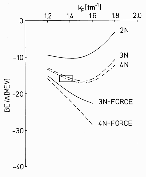
Figure 35: The curves labeled 2N, 3N, and 4N correspond to the 2-, 3-, and 4-hole-line results from Ref. [134] for the Reid interaction. Added to the 4N results are the contribution of three- and four-body ring diagrams involving at least one $\Delta$-isobar configuration. These terms can be considered as three- and four-body force contributions when only nucleons are considered are therefore labeled with 3N- and 4N-force, respectively.

This result is illustrated in Fig. 35 where these contributions are added to the hole-line expansion results from Ref. [134]. Alternatively, these terms involving $\Delta$-isobars can also be considered as contributions due to three- and four-body forces in the space of only nucleons. These $\Delta$-isobar terms have a very different behavior from the phenomenological three-body forces that have been used to describe the properties of nuclear matter [138, 139]. The latter three-body forces turn repulsive at higher density. The importance of the pionic long-range contributions to the binding energy shown in Fig. 35 is related to the possible appearance of pion condensation at higher nuclear density [158, 159]. These long-range pion-exchange dominated contributions to the binding energy appear because of conservation of momentum in nuclear matter. For a given momentum $q$ carried by a pion around a ring diagram, one is able to sample coherently the attractive interaction that exists for values of $q$ above 0.7 ${\rm fm}^{-1}$. All ring diagrams contribute coherently when the interaction is attractive and one may therefore obtain huge contributions at higher densities which reflect the importance of this collective pion-propagation mode [160]. This is clearly illustrated by the results shown in Fig. 35.

No such collective pion-degrees of freedom are actually observed in finite nuclei. A substantial part of the explanation of this fact is provided by the observation that in finite nuclei both the attractive and repulsive parts of the pion-exchange interaction are sampled before a build-up of long-range correlations can be achieved. Since these contributions very nearly cancel each other, which is further facilitated by the increased relevance of exchange terms [161], one does not see any marked effect on pion-like excited states in nuclei associated with long-range pion degrees of freedom even when $\Delta$-hole states are included [162]. It seems therefore reasonable to call into question the relevance of these coherent long-range pion-exchange contributions to the binding energy per particle since their behavior is so markedly different in finite and infinite systems. One may consider the salient difference of the ratio of spin-longitudinal and spin-transverse response function in nuclear matter and finite nuclei as another indication of the relevance of this suggestion [163]. We also like to point out that experimental information of these response functions [164] - [166] suggests no characteristic enhancement of the (pionic) spin-longitudinal response as expected on the basis of nuclear matter calculations.

Clearly, the assertion that long-range pion-exchange contributions to the energy per particle need not be considered in explaining nuclear saturation properties, needs to be further investigated. In practice, this means that one must establish whether pion-exchange in heavy nuclei already mimics the corresponding process in nuclear matter. If this does not turn out to be the case, the arguments for considering the nuclear-matter saturation problem only on the basis of the contribution of SRC will be strenghtened considerably. Furthermore, one would then also expect that the contribution of three-body forces [167] to the binding energy per particle in finite nuclei continues to be slightly attractive when particle number is increased substantially beyond ten particles [168]. This point and the previous discussion also suggest that there would be no further need for the ad-hoc repulsion added to three-body forces used to fit nuclear-matter saturation properties [138].

5 Theoretical calculations for finite nuclei

The structure of finite nuclei presents different features from the case of nuclear matter due to the fact that nucleons are localized inside the system. This requires the consideration of single particle basis states that have good total angular momentum (and parity) and correspond to discrete set of levels, as in the IPM. The coupling to low-lying collective excitations in the system tends to fragment the sp strength of these orbitals and to spread it over a wide range of energies associated with the energy scales of these excitations. Along with these effects, short-range correlations can move a sizable fraction of nucleons to high-momentum states as in the case of nuclear matter discussed in the previous section.

The influence of SRC in finite nuclei has been studied theoretically by calculating the momentum distribution in the ground state of selected nuclei [169] - [174]. These results clearly show that for momenta above 400 MeV/c short-range and tensor correlations completely dominate the momentum distribution. Although the momentum distribution is a sp quantity, and thus allows only an indirect measurement of correlations, a careful study can give some indications on the importance of these effects. More information is contained in the hole spectral function $S_{\ell j\tau}(k,E)$, which gives the distribution of nucleons both in momentum and energy for particles with orbital angular momentum $\ell$, total angular momentum $j$, and isospin $\tau$. In nuclei, substantial correlations beyond the IPM approach are present and a full understanding of the many-body system requires, both in experimental as well as theoretical studies, the knowledge of $S_{\ell j\tau}(k,E)$ for a large range of energies $E$ as will be discussed in Sec. 5.2.

Microscopic calculations of the spectral function and the momentum distribution of finite nuclei based on realistic nuclear hamiltonians have been performed for very light nuclei ($A\leq 4$) in Refs. [175] - [178]. Results for heavier nuclei are typically derived from investigations of nuclear matter assuming a local density approximation (LDA) [173, 179] -[181]. Other variational calculations for ${}^{16}{\rm O}$ yield the momentum distribution [174] and the $p$-shell quasihole wave functions [182, 183] but not the complete energy dependence of the hole spectral functions. The latter was studied by Benhar et al. [180], for different nuclei using nuclear matter results and LDA, and in Refs. [184, 151, 185] for ${}^{16}{\rm O}$ using the Green’s function formalism. These calculations suggest that most of this strength is found along a ridge in the momentum-energy plane ($k$-$E$) which spans several hundreds of MeV/c (and MeV). Moreover, although the distribution of this strength accounts only for a small fraction of the total number of nucleons, it is responsible for as much as 60% of the total binding energy of the system [151]. As a consequence, the present understanding of nuclear correlations would gain important information from the experimental knowledge of this distribution. Such experiments require a high energy transfer from the probe to the nucleus and a careful choice of the kinematics in order to minimize the final state interactions [186]. For this reason it has only recently been possible to obtain reliable experimental data in this correlated region which are still being analyzed [187, 188].

Several studies have been carried out to obtain nuclear spectral functions at small and medium missing energies, mostly by computing the many-body Green’s function [146], [189] - [197]. The qualitative features of the strength distribution at small and medium missing energies can be understood by realizing that a considerable mixing occurs between hole states and 2h1p configurations. This mixing leads to different strength patterns depending on the location of the orbital under consideration. An orbital in the immediate vicinity of the Fermi energy will still yield a large fragment near its original position since the 2h1p states are quite far in energy. For the same reason, only small components of this orbit appear at 2h1p energies. These features are observed for the $3s_{1/2}$ proton orbit in ${}^{208}\textrm{Pb}$ as shown in Fig. 36. An orbit which is surrounded by many 2h1p states will yield a strongly fragmented pattern, the width depending on the strength of the mixing interaction. These features are all observed experimentally as shown in Fig. 36.

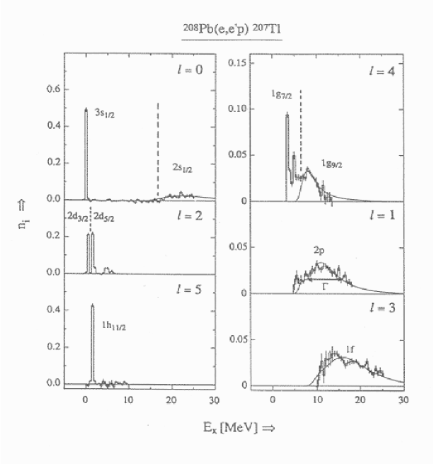
Figure 36: Spectroscopic factors from the (e,e^′p) reaction on ${}^{208}\textrm{Pb}$ for different valence hole orbits. The spectroscopic factor for the main fragment of the $3s_{1/2}$ orbit must be changed to 0.65 from the values in the figure to reflect the analysis given in Ref. [14].

The actual values of the spectroscopic strength shown in this figure have not been corrected for the effect of the Coulomb distortion on the electron. This effect is sizable in heavy nuclei and leads to an increase of the spectroscopic factor for the $3s_{1/2}$ strength to 0.65 from the values of 0.5 shown in this figure [14].

Calculations for medium-heavy nuclei like ⁴⁸Ca and ⁹⁰Zr gave a fairly good description of the fragmentation pattern of valence hole states [146] in terms of the coupling between quasiparticles and TDA/RPA collective modes. The spectroscopic factors obtained in that work typically overestimates the experimental summed strength by about a 15% if only these long-range correlations are included. The remaining surplus of strength is presumed to be moved to very high missing energies by the effects of short-range and tensor correlations as discussed in Sec. 4. This is consistent with the reduction of the occupation of low momentum states in nuclear matter also discussed in that section. This result from Ref. [61] is supported by the observation that all the removed sp strength for such small momenta in nuclear matter ends up at very high energies in the particle domain associated with the repulsive core and tensor components of the nucleon-nucleon interaction [61] (see also Sec. 4.2). Applying a corresponding adhoc reduction of the theoretical strength in medium-heavy nuclei like ${}^{48}\textrm{Ca}$ yields an overall satisfactory description of the sp strength distribution as discussed in Sec. 5.1.

The conclusion that all is well is, however, premature. The effects of SRC on the spectroscopic factors of ${}^{16}{\rm O}$ have been computed in Refs. [182] - [184]. All these works yield spectroscopic factors of 90% for the knockout of a proton for the $p_{1/2}$ and $p_{3/2}$ shells in the (e,e^′p) reaction before the effects of the spurious motion of the center-of-mass are taken into account. Such center-of-mass corrections are known to raise the theoretical spectroscopic factor by about 7% [24, 198]. These results are in disagreement with the experimental value of about 60% for these orbitals [199]. The inclusion of the coupling to 2p1h and 2h1p states at low energy has been considered in Refs. [195, 196] without leading to an explanation of this discrepancy. In particular, in Ref. [196] a successful attempt to combine the treatment of low-energy long-range and short-range (and tensor) correlations was achieved. The final result yielded a $p_{3/2}$ spectroscopic factor of 76%, while still neglecting center-of-mass corrections. This leaves a discrepancy with the experiment of about 15-20% (taking into account the quoted uncertainties). The calculations of Refs. [195, 196] take into account the interaction between the hole and particles propagating in the system at the TDA level and therefore cannot go beyond the 2h1p level. The calculation of Ref. [146] can account for the coupling of quasiparticles to RPA collective modes and therefore goes beyond 2h1p contributions, although it is limited by the difficulties in including the coupling to collective excitations in both the pp(hh) and ph channels. The effects of fragmentation (or self-consistency) were only taken into account in Ref. [190] were a fully self-consistent calculation was obtained with a satisfactory representation of the continuum. However, this calculation does not contain the coupling to collective excitations and uses a phenomenological effective interaction. A procedure to include both ph and pp(hh) excitations in the construction of the self-energy was recently proposed and implemented in Refs. [32, 197]. It was pointed out in this work that the RPA description of the excitation spectrum for ${}^{16}{\rm O}$ is quite inadequate at present and may be partly responsible for the unsatisfactory situation for ¹⁶O.

We begin this section by reviewing some early calculations for finite nuclei in Sec. 5.1. These results show that the properties of the spectral fragmentation can be understood in terms of the coupling of single particle motion to collective pp(hh) and ph motion, except for the reduction of the spectroscopic factors that is due to SRC. A method that allows the evaluation of the effects of SRC on the spectral function is reviewed in Sec. 5.2. Calculations for the particular case of ${}^{16}{\rm O}$ confirm the expected reduction of spectroscopic factors due to short-range effects. This calculation also gives quantitative information on the distribution of the correlated spectral strength. The location of this strength and the effects on the binding energy of nuclear systems are discussed on section 5.3. The formalism necessary to include the effects of both pp(hh) and ph phonons in the nuclear self-energy, while describing them at least at the RPA level, is discussed in Sec. 5.4. We present recent results for the spectral function of ${}^{16}{\rm O}$ at low missing energy in Sec. 5.5 and compare them to the available experimental data. The relation between the details of the spectral distribution and the results for the excitation spectrum allows one to identify relevant missing ingredients necessary to understand the spectroscopic factors of this nucleus. A first attempt to improve the description of the spectrum [200] is discussed in Sec. 5.6.

The two-hole spectral function can be computed, including the fragmentation effects, by solving the pp(hh) DRPA equation. The high momentum components –excluded form the model space– can be included afterwards by computing the relevant defect functions. Some results for two-nucleon emission, that clearly show the signature of SRC are discussed in Sec. 5.7. The issue of how to deal with final state interactions in reactions at high momentum transfer with regard to the extraction of spectroscopic factors is discussed in Sec. 5.8. We conclude this section by discussing two recent experiments that give the first direct experimental information of the occupation numbers of deep-lying orbitals in ${}^{208}{\rm Pb}$ and on the spectral strength distribution at high momenta, Sec. 5.9.

5.1 Early results for the spectral distribution

The earliest calculations of the spectral strength in nuclei were reported in Ref. [189, 190]. The study of the spectral strength distribution starting from a realistic NN interaction is only possible when short-range correlations are properly included. These early calculations either relied on the construction of a local $G$ matrix interaction obtained from nuclear matter [201] to represent SRC [189] or relied on phenomenological forces [190]. The latter approach actually generated the first self-consistent calculation of the spectral strength in nuclei based on the inclusion of the second-order self-energy diagram. The former calculations also used a second-order approach but included the $G$ matrix effective interaction without achieving self-consistent results. Useful insights were obtained from these calculations which described certain features of the spectral distribution obtained from the ⁴⁸Ca(e,e^′p) reaction [202]. The inclusion of SRC on the distribution of the strength was not considered in this work (see Sec. 5.2). As a general conclusion of this work on ⁴⁸Ca, it is found that the total strength in the experimentally accessible domain in the (e,e^′p) reaction is overestimated by about 10-15% although the shape of the strength distribution is already well described as shown in Fig. 38. These results for the sp strength distribution for proton removal from ${}^{48}{\rm Ca}$ in $\ell=2$ states are compared to the corresponding experimental data [202]. The theoretical results are labeled by “2nd Order” in the figure. The normalization in the figure is such that if a single state carried all the strength, the peak height at the corresponding energy would be $2j+1$. The first peak corresponds to $d_{3/2}$ removal whereas most of the rest of the strength corresponds to $d_{5/2}$ removal. The difference between the fragmentation of these two $sp$ orbitals characterizes the basic features which are found in experiment. For an orbital which in mean field is very near the Fermi energy, like the $d_{3/2}$ orbital, fragmentation of strength to all 2p1h and 1p2h-like states takes place in such a way that the distribution is characterized by a single large fragment and hundreds of tiny contributions spread out over the whole energy domain covered by the 2p1h and 1p2h states. This background contribution to the hole strength, $i.e.$ the strength which is not contained in the area of the main peak, is of the order of 10%.

The comparison between the second-order results and experiment in Fig. 38 also shows that stronger fragmentation in the theoretical calculation at low energy is required. Improvement of the description of the intermediate states in the self-energy was investigated in Ref. [146]. In this paper various possible descriptions of the intermediate 2p1h/2h1p in the self-energy were considered. This approach can be summarized by considering Fig. 37 which exhibits the diagrammatic content of these approximations.

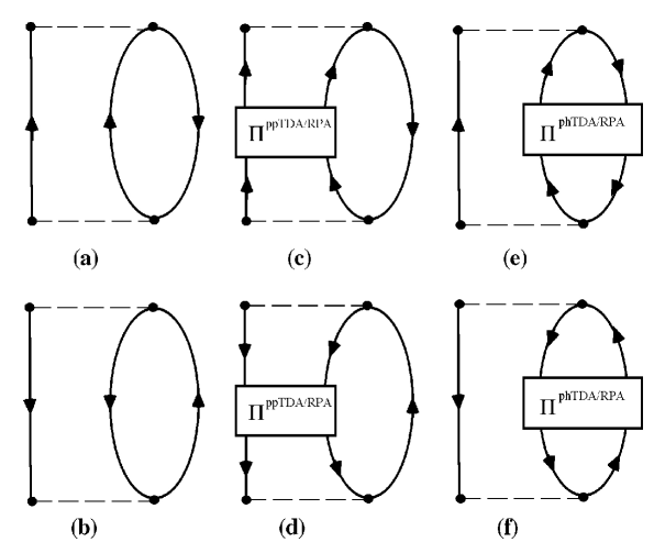
Figure 37: Second-order self-energy terms represented by Goldstone diagrams $a$ and $b$. Extensions are made by including TDA or RPA correlations in the particle-particle (diagrams $c$ and $d$) or particle-hole channel (diagrams $e$ and $f$).

These different approximations correspond to the standard versions of the TDA and RPA for both ph and pp(hh) forms as discussed in Sec. 2 and are represented by diagrams $c$ through $f$ in Fig. 37.

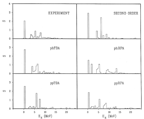
Figure 38: Distribution of $sp$ strength for $\ell=2$ proton removal from ${}^{48}{\rm Ca}$. Experimental data are from Ref. [202]. Theoretical results are displayed for various approximations to the self-energy which are discussed in the text.

These approximations include the effect of long-range (low-enery) correlations on the fragmentation pattern at low energy. It should be noted that three independent types of possible collective excitations occur, i.e. neutron particle - proton hole, proton particle - neutron hole, and a mixture of neutron particle - neutron hole and proton particle - proton hole with isospin components $T_{z}$=1, -1, and 0, respectively. The $T_{z}$=0 collective low-lying $2^{+}$ and $3^{-}$ phonons are especially relevant as their coupling to the sp motion is an important source of fragmentation of spectral functions at low energies. While collective effects are stronger in the RPA, it is possible to encounter serious problems with this method. They arise, especially in phRPA, when the RPA correlations are so strong that the lowest solution for some angular momentum and parity, has imaginary eigenvalues and the amplitudes cannot be properly normalized. This happens for the 3^- phonon, which is crucial for the fragmentation of the $\frac{7}{2}^{-}$ strength in ⁴⁸Ca. As the imaginary solution can not be included it has to be discarded and the phRPA method is unsatisfactory in this case [146]. For the same reason the lowest 1⁺ states in ⁴⁶K en ⁵⁰Sc become unstable in ppRPA and therefore were also discarded in that approach. These problems are expected to disappear when a self-consistent approach would be adopted, which has not been implemented for this nucleus sofar. The comparison of the various approximations in Fig. 38 to the experimental data shows that increased fragmentation at low energy is obtained when collective effects are considered. The sp strength farther away from the Fermi energy is largely unaffected.

The summed sp strength below the Fermi energy generates the occupation numbers for the orbits considered as given by Eq. (9). Experimentally, the hole strength has been determined only within a limited energy region. For the valence $\ell=0$ and $\ell=2$ shells the main portion of the total strength falls within this range of energies. In all theoretical approaches discussed here the calculated extra hole strength at higher energies is only 5-10$\%$ of the $2j+1$ sum rule for the 2s shell and only 10-15$\%$ for the 1d shell. For the major shells above the Fermi level the occupation probability is about 5-10$\%$ and for more remote shells only 1-2$\%$. A meaningful quantity is the jump in occupation numbers at the Fermi level. This jump in occupation number for the ppTDA result is 0.74. In Fig. 39 these occupation numbers in the ppTDA approximation are multiplied by a factor of 0.9 to simulate the effect of SRC.

Figure 39: Proton shell occupation probabilities deduced from a comparison of the present calculation and the (e,e^′p) data [202]. The figure displays the calculated values with the ppTDA correlations in the self-energy, multiplied by a factor 0.9 to simulate the effect of short-range correlations.

The resulting occupation numbers show a flat behavior for deeply bound shells while they bend down when the orbits approach the Fermi energy. This feature also emphasizes that LRC are most important in the immediate vicinity of the Fermi energy.

5.2 Depletion due to short-range and tensor correlations

The treatment of short-range correlations requires the consideration of the details of the two-particle wave function at small internucleon distances (or high relative momenta). This suggests that it is appropriate to work directly in coordinate or momentum space. The approach introduced in Refs. [203, 184, 151] computes the self-energy for finite nuclei in terms of a $G$-matrix which is obtained as a solution of the Bethe-Goldstone equation for nuclear matter

$$\left\langle k\ell\right|G_{SJ_{S}KLT}\left|k^{\prime}\ell^{\prime}\right\rangle=\left\langle k\ell\right|V\left|k^{\prime}\ell^{\prime}\right\rangle$$ (133)

$$+\sum_{\ell^{\prime\prime}}\int dk^{\prime\prime}(k^{\prime\prime})^{2}\;\left\langle k\ell\right|V\left|k^{\prime\prime}\ell^{\prime\prime}\right\rangle\frac{Q(k,K)}{\omega_{NM}-\frac{K^{2}}{4m}-\frac{k^{2}}{2m}}\left\langle k^{\prime\prime}\ell^{\prime\prime}\right|G_{SJ_{S}KLT}\left|k^{\prime}\ell^{\prime}\right\rangle\;,$$

where $k$, $k^{\prime}$, and $k^{\prime\prime}$ denote the relative momenta between the two nucleons, $\ell$, $\ell^{\prime}$, and $\ell^{\prime\prime}$ the orbital angular momenta for the relative motion, $K$ and $L$ the corresponding quantum numbers for the center-of-mass motion, $S$ and $T$ the total spin and isospin, and $J_{S}$ is obtained by coupling the orbital angular momentum of the relative motion to the spin $S$. We note that Eq. (133) is analogous to the ladder equation for the vertex function $\Gamma$, Eq. (59a), except that it describes the intermediate propagation of two free nucleons (instead of dressed propagators), taking into account only the effects of Pauli blocking with regard to the free Fermi gas. This equation differs from the usual $T$-matrix of the two-body scattering problem only because of the inclusion of the Pauli operator $Q$ that prevents the two nucleons to scatter into states inside the Fermi sea (which are already occupied). Equation (133) therefore generates an appropriate solution of two-body short-range dynamics. The choices for the density of nuclear matter and the starting energy $\omega_{NM}$ are rather arbitrary. The calculation of the corresponding Hartree-Fock term is not very sensitive to this choice [204]. Furthermore, this nuclear-matter approximation is corrected by calculating the 2p1h term displayed in Fig. 40(b) directly for the finite system. This second-order correction, which assumes harmonic oscillator states for the occupied (hole) states and plane waves for the intermediate unbound particle states, incorporates the correct energy and density dependence characteristic of a finite nucleus $G$-matrix.

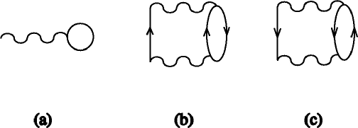
Figure 40: Graphical representation of the Hartree-Fock (a), the 2-particle 1-hole (2p1h, b) and the 2-hole 1-particle contribution (2h1p, c) to the self-energy of the nucleon.

To evaluate the diagrams in Fig. 40, one requires matrix elements in a mixed representation of one particle in a bound harmonic oscillator while the other is in a plane wave state. Using vector bracket transformation coefficients [205], one can transform matrix elements from the representation in coordinates of relative and center-of-mass momenta to the coordinates of sp momenta in the laboratory frame in which the two particle state is described by

$$\left|k_{1}\ell_{1}j_{1}k_{2}\ell_{2}j_{2}JT\right\rangle,$$ (134)

where $k_{i}$, $\ell_{i}$ and $j_{i}$ refer to the momentum and angular momenta of particle $i$ whereas $J$ and $T$ define the total angular momentum and isospin of the two-particle state. Performing an integration over one of the $k_{i}$, one obtains a two-particle state in a mixed representation

$$\left|n_{1}\ell_{1}j_{1}k_{2}\ell_{2}j_{2}JT\right\rangle=\int_{0}^{\infty}dk_{1}\,k_{1}^{2}R_{n_{1},\ell_{1}}(k_{1})\,\left|k_{1}\ell_{1}j_{1}k_{2}\ell_{2}j_{2}JT\right\rangle\;.$$ (135)

Here $R_{n_{1},\ell_{1}}$ stands for the radial oscillator function and the oscillator length is chosen to be $b=1.72$ fm^-1 to achieve an appropriate description of the bound states of ${}^{16}{\rm O}$. Using the results of Eqs. (133) - (135) the Hartree-Fock approximation for the self-energy can be obtained in the momentum representation

$$\Sigma^{HF}_{\ell_{1}j_{1}}(k_{1},k^{\prime}_{1})=\frac{1}{2(2j_{1}+1)}\sum_{n_{2}\ell_{2}j_{2}}\sum_{JT}(2J+1)(2T+1)\left\langle k_{1}\ell_{1}j_{1}n_{2}\ell_{2}j_{2}\right|G_{JT}\left|k^{\prime}_{1}\ell_{1}j_{1}n_{2}\ell_{2}j_{2}\right\rangle.$$ (136)

The summation over the oscillator quantum numbers is restricted to the states occupied in the IPM of ¹⁶O. This Hartree-Fock part of the self-energy is real and does not depend on the energy.

The terms of lowest order in $G$ which give rise to an imaginary part in the self-energy are represented by the diagrams displayed in Figs. 40(b) and 40(c), refering to intermediate 2p1h and 2h1p states, respectively. The 2p1h contribution to the imaginary part is given by

$${W}^{2p1h}_{\ell_{1}j_{1}}(k_{1},k^{\prime}_{1};E)=\frac{-1}{2(2j_{1}+1)}\sum_{n_{2}\ell_{2}j_{2}}\sum_{\ell L}\sum_{JST}\int k^{2}dk\int K^{2}dK\;(2J+1)(2T+1)$$

$$\times\left\langle k_{1}\ell_{1}j_{1}n_{2}\ell_{2}j_{2}\right|G_{JT}\left|k\ell SKL\right\rangle\left\langle k\ell SKL\right|G_{JT}\left|k^{\prime}_{1}\ell_{1}j_{1}n_{2}\ell_{2}j_{2}\right\rangle\;\pi\;\delta\left(E+\varepsilon_{n_{2}\ell_{2}j_{2}}-\frac{K^{2}}{4m}-\frac{k^{2}}{m}\right),$$

where the average experimental quasihole energies $\varepsilon_{n_{2}\ell_{2}j_{2}}$ are used for the hole states ($-47$ MeV, $-21.8$ MeV, $-15.7$ MeV for $s_{1/2}$, $p_{3/2}$ and $p_{1/2}$ states, respectively), while the energies of the particle states are given in terms of the kinetic energy only. The plane waves associated with the particle states in the intermediate states are properly orthogonalized to the bound sp states following the techniques discussed in Ref. [203]. The 2h1p contribution to the imaginary part ${W}^{2h1p}_{\ell_{1}j_{1}}(p_{1},p^{\prime}_{1};E)$ can be calculated in a similar way [203].

The choice of pure kinetic energies for the particle states in calculating the imaginary parts of $W^{2p1h}$ (Eq. (LABEL:eq:w2p1h)) and $W^{2h1p}$ may not be very realistic for the excitation modes at low energy. Indeed a sizeable imaginary part in $W^{2h1p}$ is obtained only for energies $E$ below -40 MeV. However, when the primary interest is in the effects of short-range correlations, the choice appears appropriate since these involve excitations of particle states with high momenta. A different approach is required to treat the coupling to the very low-lying 2p1h and 2h1p states in an adequate way, as discussed in Secs. 5.1 and 5.4. The 2p1h contribution to the real part of the self-energy can be calculated from the imaginary part $W^{2p1h}$ using a dispersion relation [206]

$$V^{2p1h}_{\ell_{1}j_{1}}(k_{1},k_{1}^{\prime};E)=\frac{\mathcal{P}}{\pi}\int_{-\infty}^{\infty}\frac{W^{2p1h}_{\ell_{1}j_{1}}(k_{1},k_{1}^{\prime};E^{\prime})}{E^{\prime}-E}dE^{\prime},$$ (138)

where $\mathcal{P}$ stands for a principal value integral. A similar dispersion relation holds for $V^{\rm 2h1p}$ and $W^{\rm 2h1p}$.

Since the Hartree–Fock contribution $\Sigma^{\rm HF}$ has been calculated in terms of a nuclear matter $G$-matrix, it already contains 2p1h terms of the kind displayed in Fig. 40(b). In order to avoid this overcounting of the pp ladder terms, one subtracts from the real part of the self-energy a correction term ($V_{\rm c}$), which just contains the 2p1h contribution calculated in nuclear matter. Summing up the various contributions one obtains the following expression for the self-energy

$$\Sigma=\Sigma^{\rm HF}+\Delta\Sigma=\Sigma^{\rm HF}+\left(V^{\rm 2p1h}-V_{\rm c}+V^{\rm 2h1p}\right)+\left(W^{\rm 2p1h}+W^{\rm 2h1p}\right)\;.$$ (139)

The Dyson equation (13) for this self-energy can be solved in momentum space. In Ref. [151] the integrals were discretized by considering a complete basis within a spherical box of a radius $R_{\rm box}$. The calculated observables are independent of the choice of $R_{\rm box}$, if it is chosen to be around 15 fm or larger. By taking into account the different normalization of these basis functions from the case of plane waves in the continuum, one can express the matrix elements of nucleon self-energy in the “box” basis. Energies and wave functions of the quasihole states can be determined by diagonalizing the Hartree-Fock Hamiltonian plus $\Delta\Sigma$ in this “box basis” [see Eq. (37)]:

$$\sum_{n=1}^{N_{\rm max}}\left\langle k_{i}\right|\frac{k_{i}^{2}}{2m}\delta_{in}+\Sigma^{\rm HF}_{\ell j}+\Delta\Sigma_{\ell j}(E=\varepsilon^{qh}_{n-\ell j})\left|k_{n}\right\rangle\left\langle k_{n}|z^{n-}\right\rangle_{\ell j}=\varepsilon^{qh}_{n-\ell j}\ \left\langle k_{i}|z^{n-}\right\rangle_{\ell j}\;.$$ (140)

In this approach $\Delta\Sigma$ only contains a sizable imaginary part for energies $E$ below the quasihole eigenvalues $\varepsilon^{qh}_{n-\ell j}$ ($n-$ identifying discrete solutions). Therefore the solutions of Eq. (140) are separated in energy from the continuum contribution to the spectral function. The eigenvector corresponding to these discrete states yields the quasihole wave function $\left\langle k|z^{n-}\right\rangle_{\ell j}$ in momentum space, which still needs to be normalized by the spectroscopic factor $Z^{qh}_{n-\ell j}$ by means of Eq. (38). The diagonal part of the quasihole contribution to the spectral function is given, in the box basis, by

$$S^{qh}_{n-\ell j}(k_{n};E)=Z^{qh}_{n-\ell j}\left|\left\langle k_{n}|z^{n-}\right\rangle_{\ell j}\right|^{2}\,\delta(E-\varepsilon^{qh}_{n-\ell j})\;.$$ (141)

In the calculations described in Refs. [151, 185], the Bethe-Goldstone equation (133) was solved by employing for $V$ the one-boson-exchange potential Bonn-$B$ developed by Machleidt in Ref. [207] (Tab. A.2) and the Pauli operator $Q$ was approximated by the so-called angle-averaged approximation for nuclear matter with a Fermi momentum $k_{F}=1.4\ \textrm{fm}^{-1}$. This roughly corresponds to the saturation density of nuclear matter. The starting energy $\omega_{NM}$ for computing the $G$-matrix, Eq. (133), was chosen to be -10 MeV.

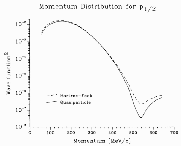
Figure 41: Square of the quasihole wave function for the $p_{1/2}$ state in ${}^{16}{\rm O}$ (full curve), normalized to the spectroscopic factor according to Eq. (38), compared to the Hartree-Fock result (dashed curve).

The square of the quasihole wave function for the $p_{1/2}$ state (normalized to the spectroscopic factor, $Z^{\rm qh}_{0p1/2}$) is shown in Fig. 41 as a full line. For comparison the result for the Hartree-Fock wave function is shown by the dashed line. From the comparison one can infer that at the quasihole energies no substantial change in the wave functions occurs and that the Hartree-Fock wave function is a good approximation. It should be further noted that the wave function of a Woods-Saxon potential, which is constructed as the local equivalent of the Hartree-Fock potential [203], is indistinguishable from the Hartree-Fock wave function. This suggests that the explicit inclusion of short-range correlations does not lead to the strong suppression of the wave function in the interior of the nucleus as has been suggested by Refs. [208, 39]. These findings are in line with the observation that the quasiholes representing mean-field orbitals can be adequately described by a local potential [25]. It should be emphasized that this is not necessarily the case for other overlap functions [25], since the coupling to collective excitations can lead to significant changes to the quasihole wave function [25, 209]. These effects are unlikely to generate changes in the high-momentum components discussed here. It is important to note that these results also show that the influence of high-momentum components in the quasihole wave function is of minor importance, so the enhancement of the momentum distribution has to come from excitations at higher missing energies.

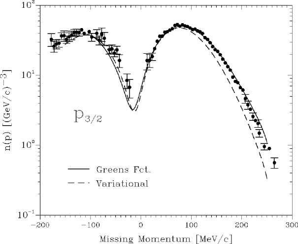
Figure 42: Reduced cross section for the ¹⁶O$(e,e^{\prime}p)$ reaction in parallel kinematics leading to the ${3/2}^{-}$ state at $-6.32$ MeV of the residual nucleus ¹⁵N. Results of the Green’s function approach (solid line) are compared to those obtained in the variational calculation of Ref. [182] (dashed line) and the experimental data [199]. A spectroscopic factor of 0.537 was required for the Green’s function result, while $Z_{0p3/2}=0.459$ has been used to for the variational calculation.

We show in Fig. 42 an example of the reduced cross section for the (e,e^′p) reaction on ¹⁶O leading to bound quasihole state of ¹⁵N at an excitation energy of $-6.32$ MeV [210]. In this picture the effects of FSI have been computed in the distorted wave impulse approximation (DWIA) [17] and the data points have been obtained at NIKHEF for the so-called parallel kinematics [199]. Using the quasihole part of the spectral function computed from Eq. (140) but adjusting the spectroscopic factor for the quasihole state contribution $Z^{qh}_{0p3/2}$ to fit the experimental data, one obtains the solid line of Fig. 42. Comparing this result with the experimental data one finds that the calculated spectral function reproduces the shape of the reduced cross section as a function of the missing momentum quite well. The absolute value for the reduced cross section can only be reproduced by employing a spectroscopic factor $Z^{qh}_{0p{3/2}}=0.537$, a value considerably below the one of 0.914 calculated using Eq. (140) [151]. An analogous result holds for transition to the $p_{1/2}$ ground state of ¹⁵N for which the same analysis yields a spectroscopic factor $Z^{qh}_{0p{1/2}}=0.644$. For comparison, one may note that the use of phenomenological Woods-Saxon wave functions adjusted to fit the shape of the reduced cross section require spectroscopic factors ranging from 0.61 to 0.64 for the lowest $0p_{1/2}$ state and from 0.50 to 0.59 for the $0p_{3/2}$ state, respectively, depending upon the choice of the optical potential for the outgoing proton [199].

Figure 42 also contains the results for the reduced cross section derived from the variational result for overlap wave function of Pieper et al. [182], who employed the Argonne $v_{14}$ potential for the NN interaction [136]. Also in this case the shape of the experimental data is globally reproduced with a slightly better agreement for small negative values of $p_{m}$ but with a clear underestimation at larger $p_{m}$. The overall quality of the fit is somewhat worse than for the Green’s function approach and the required adjusted spectroscopic factor is $Z^{qh}_{0p_{3/2}}=0.459$, below the value of 0.537 for the latter approach. It is not clear, however, whether the differences in the calculated reduced cross section are due to the use of different interactions or to the methods employed in calculating the spectral function.

Both the variational calculations of Refs. [182, 183] and the Green’s function approach give spectrocsopic factors for the $p$-shell orbitals of about 0.90. This value should be compared to the $\sim$0.63 obtained form the NIKHEF experimenf for these shells. The additional contribution due to the proper consideration of the center-of-mass motion raises the theoretical value to 0.98, worsening the agreement with data [198]. Nevertheless, the observation that the same results are obtained with two independent many-body methods but including the same short-range physics suggests that the effects of SRC on the quasihole strength are well under control. At the same time, the discrepancy with the experiment is partly due to the emphasis on the accurate treatment of short-range correlations only and one should view the quasihole strength that has been discussed here to be due only to the influence of short-range correlations [203]. It is clear that a considerable renormalization of the strength is to be expected due the coupling of the quasihole states to the low-lying collective excitations, as will be discussed in Sec. 5.5.

5.3 High-momentum components at high missing energies

The continuum part of the hole spectral strength is found at higher energies and stems from the coupling to the continuum of 2h1p states. In this region it is useful to proceed from the Hartree-Fock propagator with states $\left|\alpha\right\rangle$ that diagonalize the corresponding self-energy

$$g_{\ell j}^{(0)}(\alpha;E)=\frac{1}{E-\varepsilon^{HF}_{\alpha\ell j}\pm i\eta},$$ (142)

where the sign in front of the infinitesimal imaginary quantity $i\eta$ is positive (negative) depending on whether $\varepsilon^{HF}_{\alpha\ell j}$ is above or below the Fermi energy. The Dyson equation can then be solved by iterating the $\Delta\Sigma$ component in Eq. (139) of the self-energy to generate the reducible self-energy

$$\left\langle\alpha\right|\Sigma^{red}_{\ell j}(E)\left|\beta\right\rangle=\left\langle\alpha\right|\Delta\Sigma_{\ell j}(E)\left|\beta\right\rangle+\sum_{\gamma}\left\langle\alpha\right|\Delta\Sigma_{\ell j}(E)\left|\gamma\right\rangle g_{\ell j}^{(0)}(\gamma;E)\left\langle\gamma\right|\Sigma^{red}_{\ell j}(E)\left|\beta\right\rangle$$ (143)

and obtain the propagator from

$$g_{\ell j}(\alpha,\beta;E)=\delta_{\alpha,\beta}\ g_{\ell j}^{(0)}(\alpha;E)+g_{\ell j}^{(0)}(\alpha;E)\left\langle\alpha\right|\Sigma^{red}_{\ell j}(E)\left|\beta\right\rangle g_{\ell j}^{(0)}(\beta;E).$$ (144)

Using this representation of the Green’s function one can calculate the spectral function in the “box basis” from [see Eq.(4)]

$$S_{\ell j}^{c}(k_{n};E)=\frac{1}{\pi}\ \mbox{Im}\left(\sum_{\alpha,\beta}\left\langle k_{n}|\alpha\right\rangle_{lj}\;g_{lj}(\alpha,\beta;E)\,\left\langle\beta|k_{n}\right\rangle_{lj}\right).$$ (145)

This spectral function is different from zero for energies $E$ below the lowest sp energy of a given Hartree-Fock state (with $\ell j$) only due to the imaginary part in $\Sigma^{red}$. This contribution involves the coupling to the continuum of 2h1p states and is therefore nonvanishing only for energies at which the corresponding irreducible self-energy $\Delta\Sigma$ has a non-zero imaginary part. The 2p1h contribution to the self-energy is responsible for the depletion of strength, which in mean field is located below the Fermi energy, to high energy. The 2h1p term instead, is essential for the accumulation of sp strength below the Fermi energy from states (in particular those with high momenta) which are empty in the mean field. The continuum contribution of Eq. (145) and the quasihole parts of Eq. (141), which are obtained in the basis of box states, can be added and renormalized to obtain the complete spectral function in the continuum representation at the momenta defined by the box basis from

$$S_{\ell j}(k_{i};E)=\frac{2}{\pi}\ \frac{1}{N_{i\ell}^{2}}\bigl{(}S^{c}_{\ell j}(k_{i};E)+\sum_{n-}S^{qh}_{n-\ell j}(k_{i};E)\bigr{)},$$ (146)

where the $N_{i\ell}$ correspond to appropriate normalization constants [151].

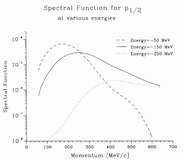
Figure 43: The $p_{1/2}$ spectral strength as a function of momentum at fixed energies corresponding to -50, -150, and -250 MeV. The results demonstrate the increasing importance of high-momentum components with higher excitation energy in the $A-1$ system.

The results for the spectral function $S_{\ell j}^{c}(k;\omega)$ for the $p_{1/2}$ quantum numbers are shown at three different energies in Fig. 43. The long-dashed curve corresponds to -50 MeV, the full curve to -150 MeV, and finally the short-dashed curve to -250 MeV. From these results it is clear that an important change in the momentum content of the sp strength occurs with increasing excitation energy in the $A=15$ system. At higher excitation energy one finds more high-momentum components. Moreover, these high-momentum components are not observed in the quasihole states. This can be concluded by considering Fig. 44 where the total momentum distribution, including the contribution from the quasihole states, is shown in the left panel. This requires the energy integration of the continuum hole strength for each $k$ according to Eq. (9). This distribution is presented for various energy cut-offs. The quasihole part reflects the cross section for knockout reactions with small energy transfer, i.e. leading to the ground state of the final nucleus and excited states up to $\approx 20$ MeV. The curve denoted by $E>$ -100 MeV reflects the momentum distribution including all states of the final nucleus up to around 80 MeV, etc. This result for ${}^{16}{\rm O}$ is very similar to the observation for ${}^{3}{\rm He}$ made in Ref. [176], where the contribution of the ground state to ground state transition exhibits also very few high-momentum components. As a consequence the high-momentum components of the momentum distribution due to short-range correlations can be observed mainly in knockout experiments with an energy transfer of the order of 100 MeV or more. The right panel of Fig. 44 compares the total momentum distribution for ${}^{16}{\rm O}$ obtained with different approaches, and different interactions, all of which properly include the effects of short-range correlations [185].

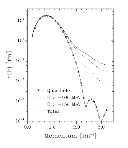
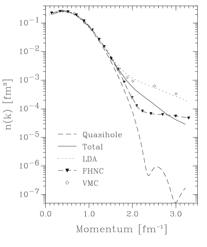
Figure 44: The total momentum distribution of ¹⁶O. The left panel also displays the quasihole contribution and the results obtained with various energy cut-offs in the integration of the spectral functions. The right panel compares the momentum distribution obtained with the Green’s function (total) with that of other approaches: local density approximation (LDA) [180], Fermi hypernetted chain (FHNC) [211] and Variational Monte Carlo (VMC) [174]. It should be noted that different normalizations were used for the presentation of these panels.

To understand this result, it is important to recall that the appearance of high-momentum components at a certain energy in the $A-1$ system is related to the self-energy contribution containing 2h1p states at this energy. From energy conservation it is then clear that at low energy it is much harder to find such states with a high-momentum particle than at high energy. This same feature is observed in nuclear matter where the peak of the sp spectral function for momenta above $k_{F}$ increases in energy as $k^{2}$ [212]. As a result, the hole strength in nuclear matter as a function of momentum shows the same tendency as the result shown in Fig. 43 [66], i.e. higher momenta become more dominant at higher excitation energy.

In order to show the importance of the continuum part of the spectral functions as compared to the quasihole contribution and to visualize the effects of correlations, we have included in Tab. 1 the particle numbers for each partial wave including the degeneracy of the states

$${\hat{n}_{\ell j}}=2(2j+1)\int_{-\infty}^{\varepsilon_{F}}dE\,\int_{0}^{\infty}dk\,k^{2}S_{\ell j}(k,E)\;,$$ (147)

also separating the contributions originating from the quasihole states and those due to the continuum [as in Eq. (146)]. As already noticed above only 14.025 out of the 16 nucleons of ¹⁶O occupy the quasihole states in this calculation (while the experimental data suggests a much smaller number). Another 1.13 nucleons are found in the 2h1p continuum with partial wave quantum numbers of the $s$ and $p$ shell, while an additional 0.687 nucleons are obtained from the continuum with orbital quantum numbers of the $d$ and $f$ shells. The distinction between quasihole and continuum contributions is somewhat artificial for the $s_{1/2}$ orbital since the coupling to low-lying 2h1p states leads to a strong fragmentation of the strength [213], which is also observed experimentally [214]. It should be noted that the depletion of the occupation probabilities of the hole states, indicated in Tab 1, is larger for the $s_{1/2}$ orbit. This feature can be ascribed to the closeness of the $s_{1/2}$ Hartree-Fock energy to the 2h1p continuum which yields more leakage of strength to the continuum than for the $p_{1/2}$ and $p_{3/2}$ quasihole states. The sum of the particle numbers listed in Tab. 1 is slightly smaller (15.841) than the number particle in ¹⁶O this due to the fact that only partial waves up to $\ell=3$ were taken into account [215]. One must also keep in mind that the approach to the sp Green’s function discussed here is not number-conserving, as the Green’s functions used to evaluate the self-energy are not determined in a self-consistent way, as dicussed in Sec. 2.3.

$lj$	$\hat{n}^{qh}$	$\hat{n}^{c}(E<-150)$	$\hat{n}^{c}(E<-100)$	$\hat{n}^{c}$	$\hat{n}$	$\hat{n}/(2(2j+1))$
$s_{1/2}$	3.120	0.033	0.244	0.624	3.744	0.936
$p_{3/2}$	7.314	0.032	0.133	0.332	7.646	0.956
$p_{1/2}$	3.592	0.026	0.086	0.173	3.764	0.941
$d_{5/2}$	0.0	0.033	0.106	0.234	0.234	0.020
$d_{3/2}$	0.0	0.036	0.108	0.196	0.196	0.025
$f_{7/2}$	0.0	0.025	0.063	0.117	0.117	0.007
$f_{5/2}$	0.0	0.032	0.084	0.140	0.140	0.012
$\sum$	14.025	0.217	0.824	1.816	15.841

Table 1: Distribution of nucleons in ¹⁶O. Listed are the total occupation number $\hat{n}$ for various partial waves [see Eq. (147)] but also the contributions from the quasihole ($\hat{n}^{qh}$) and the continuum part ($\hat{n}^{c}$) of the spectral function, separately. The continuum part is split further into contributions originating from energies $E$ below -150 MeV ($n^{c}(E<-150)$) and from energies below -100 MeV. The last line shows the sum of particle numbers for all partial waves listed.

	HF			BHF			Total
$lj$	$\epsilon$	$t$	$\Delta E$	$\epsilon$	$t$	$\Delta E$	$\epsilon$	$t$	$\Delta E$
$s_{1/2}$ qh	-36.91	11.77	-50.28	-42.56	11.91	-61.30	-34.30	11.23	-35.98
$s_{1/2}$ c							-90.36	17.09	-22.89
$p_{3/2}$ qh	-15.35	17.62	9.08	-20.34	18.95	-5.59	-17.90	18.06	0.37
$p_{3/2}$ c							-95.19	35.19	-9.96
$p_{1/2}$ qh	-11.46	16.63	10.34	-17.07	18.46	2.76	-14.14	17.19	5.47
$p_{1/2}$ c							-103.62	35.94	-5.84
$l>1$ c							-98.87	63.17	-12.27
$E/A$(MeV)	-1.93			-4.01			-5.12
$\left\langle r\right\rangle$(fm)	2.59			2.49			2.55

Table 2: Ground-state properties of ¹⁶O. Listed are the energies $\epsilon$ and kinetic energies $t$ of the quasihole states (qh) and the corresponding mean values for the continuum contribution (c), normalized to 1, for the various partial waves. Multiplying the sum: $\frac{1}{2}(t+\epsilon)$ of these mean values with the corresponding particle numbers of Tab.I, one obtains the contribution $\Delta E$ to the energy of the ground state [as given by the Migdal-Galitski-Koltun sumrule, Eq. (12)]. Summing up all these contributions and dividing by the nucleon number yields the energy per nucleon $E/A$. Furthermore, the rms radius for nucleon distribution is shown. Results are presented for the Hartree-Fock (HF), Brueckner-Hartree-Fock (BHF) and the complete calculation of Secs. 5.2 and 5.3 (Total). The particle numbers for the qh states in HF and BHF are equal to the degeneracy of the states, all other occupation numbers are zero. All the energies are given in MeV.

The contributions to the total energy, as derived from the Migdal-Galitski-Koltun sume rule (12), are shown in Tab. 2 for different angular momenta. The first two columns give the analogous results obtained from the solution of the Hartree-Fock (HF) and Brueckner-Hartree-Fock (BHF) terms. The latter result includes the 2p1h correction to the nuclear-matter $G$-matrix (see Ref. [151]). The BHF result continues to describe the nucleus in terms of fully occupied sp states as in HF. However, as the sp states in BHF are more bound, the gain in binding energy from HF to BHF is accompanied by a reduction of the calculated radius of the nucleon distribution. The inclusion of the 2h1p contributions to the self-energy in the complete calculation reduces the absolute values of the quasihole energies (compare BHF and “Total” in Tab. 2). Despite this reduction of the quasihole energies, however, the total binding energy is increased as compared to BHF. This increase of the binding energy is mainly due to the continuum part of the spectral function. Comparing various contributions to the intergral in Eq. (12), one finds that only 37% of the total energy is due to the quasiholes Eq. (141). The dominating part (63%) results from the continuum part of the spectral functions although this continuum part only represents 1.8 nucleons (that is 11% of the total, see Tab. 1).

Summarizing, the calculation of the complete energy dependence of the hole spectral function demonstrates that the presence of high-momentum components in the nuclear ground state will only show up unambiguously at high excitation energy when probed by $(e,e^{\prime}p)$ reactions. These deeply bound nucleons, not only generate the enhancement of the momentum distribution for momenta $>400$Mev/c, depicted in Fig. 44, but they are essential in understanding the binding of nuclear systems. More discussion of these high-momentum components is given in Sec. 5.9.

5.4 Faddeev approach to the treatment of collective excitations

The results for the spectroscopic factors of Sec. 5.1 demonstrate that the understanding of the occupation of quasihole states, can only be achieved with a complete description of the coupling to the low-energy collective motion of the system. In this section, we review a method that has been recently developed in Refs. [32, 197], with the aim of pursuing a complete description of these features.

The degrees of freedom that contribute to long-range correlations can be very complicated. However, when one is interested in the dynamics at small missing energies, close to the Fermi level, the problem can be simplified by focusing only on the excitations at low energy, generally a small number. If the other phonons away from the Fermi surface are high in energy they can be expected to mix weakly or not at all with the low-energy configurations. It is important to observe that this picture can be too optimistic if one works in terms of particle and hole orbitals as generated by an IPM. For example the direct diagonalization of the nuclear hamiltonian in a shell-model basis requires the inclusion of configurations at rather high energy (several $\hbar\omega$), while still obtaining sizable mixing of strength in the lowest excited states (see for example Ref. [216]). In this respect, the Green’s function approach appears to account more easily for the shift in energy of the nuclear strength, as discussed in relation to the results of Fig. 38. The coupling to 2p1h fragments is responsible for moving sizable amounts of strength into the particle domain, even at of several tens of MeVs from its original location. This mixing comes into the sp propagator through the solution of the Dyson equation and therefore it is included in the description of the low-energy excitations. One thus expects that the dressed propagator represents a more accurate approximation of the sp excitations. As a result, the decoupling between low-energy excitations and those at higher energy is more effectice when the full fragmentation of the spectral strength is taken into account, as in the SCGF theory. To some extent, the use of fragmented propagators corresponds to expanding the wave function in terms of an already correlated single particle basis, as in the Monte Carlo shell model of Ref. [217]. From a more practical point of view, the energy distribution of the spectral function and the quenching of the spectroscopic factors act as to renormalize the interaction between quasiparticles and phonons (the real degrees of freedom in the system) allowing for a better convergence of the results. A second motivation to follow the approach of SCGF comes from the observation that a fully self-consistent calculation guarantees the fulfillment of the basic conservation laws and sum rules (see Sec. 2.3) [30, 31].

In general, one may need to allow the sp motion to couple to both pp(hh) and ph motion and at the same time achieve a satisfactory description of these collective phonons. It has been known for a long time that the excitation spectrum of ¹⁶O, as obtained in TDA approximation, is particularly inadequate. In order to account for the coupling to collective excitations that are actually observed in this nucleus it is necessary to at least consider an RPA description of the isoscalar negative parity states [162]. To account for the low-lying isoscalar positive parity states an even more complicated treatment will be required. Sizable collective effects are also present in the pp and hh excitations involving tensor correlations for isoscalar and pair correlations for isovector states. Each of the diagrams $c$) to $f$) of Fig. 37 represents one of these couplings in a separate way. Moreover one must also remember that the diagrams coupling the ph and sp channel are affected by a violation of the Pauli principle already at the 2p1h/2h1p level, due to neglect of the exchange between the freely propagating hole or particle with the one propagating inside the ph phonon. More serious inconsistencies show up if one naively sums the above diagrams, with the intent of accounting for both pp(hh) and ph collective modes. In this case a double counting of the second order diagrams, Fig. 37$a$) and $b$), would come into play and there is no simple way to correct for this except to introduce spurious poles in the self-energy [32]. Therefore the inclusion of both the pp (hh) and ph collective phonons does require a complete treatment by summing these excitations to all orders. Such an expansion sums a series of diagrams like the one shown in Fig. 45. The interplay between the various phonons would ultimately generate an expansion of the 2p1h/2h1p propagator $R(\omega)$ [see Sec. 2.2] that automaically resolves the above issues. In Ref. [32], it was shown that this all order summation can by achieved by extending the technique of the Faddeev equations for the three-body problem [218, 219, 220] to the case of three interacting quasiparticle excitations. A corresponding approximation for the self-energy can then be obtained from Eq. (19).

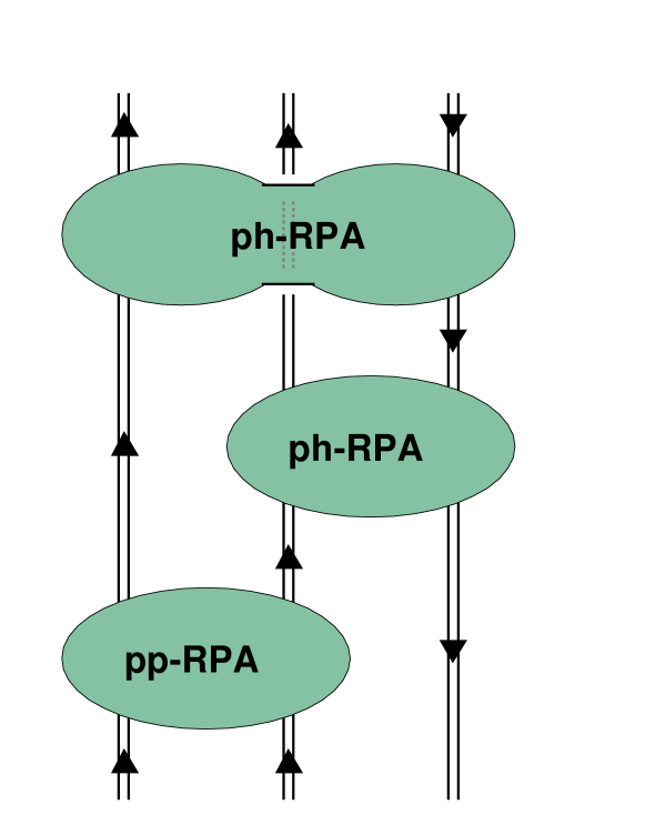
Figure 45: Example of diagrams that are summed to all orders by means of the Faddeev equations.

To describe the formalism of the Faddeev equations as applied to the many-body case, we consider the Bethe-Salpeter equation for the 2p1h propagator [which is analogous to Eq. (21) for the ph case]. In the time formulation, one has

$$R_{\mu\nu\lambda,\alpha\beta\gamma}(t_{1},t_{2},t_{3};t^{\prime})$$ (148)

$$= g_{\mu\alpha}(t_{1}-t^{\prime})g_{\nu\beta}(t_{2}-t^{\prime})g_{\gamma\lambda}(t^{\prime}-t_{3})~{}-~{}g_{\nu\alpha}(t_{2}-t^{\prime})g_{\mu\beta}(t_{1}-t^{\prime})g_{\gamma\lambda}(t^{\prime}-t_{3})$$

$$+g_{\mu\mu^{\prime}}(t_{1}-t_{1}^{\prime})g_{\nu\nu^{\prime}}(t_{2}-t_{2}^{\prime})g_{\lambda^{\prime}\lambda}(t_{3}^{\prime}-t_{3})$$

$$~{}\times\;K_{\mu^{\prime}\nu^{\prime}\lambda^{\prime},\alpha^{\prime}\beta^{\prime}\gamma^{\prime}}(t_{1}^{\prime},t_{2}^{\prime},t_{3}^{\prime};t_{4}^{\prime},t_{5}^{\prime},t_{6}^{\prime})\;R_{\alpha^{\prime}\beta^{\prime}\gamma^{\prime},\alpha\beta\gamma}(t_{4}^{\prime},t_{5}^{\prime},t_{6}^{\prime};t^{\prime})\;,$$

where here and in the rest of this section we use the convention of summing over all repeated indices and integrate from $-\infty$ to +$\infty$ over all repeated time variables, unless specified otherwise. The interaction vertex is given by

$$K_{\mu\nu\lambda,\alpha\beta\gamma}(t_{1},t_{2},t_{3};t_{4},t_{5},t_{6})$$ (149)

$$= K^{(ph)}_{\nu\lambda,\beta\gamma}(t_{2},t_{3};t_{5},t_{6})g^{-1}_{\mu\alpha}(t_{1}-t_{4})~{}+~{}K^{(ph)}_{\mu\lambda,\alpha\gamma}(t_{1},t_{3};t_{4},t_{6})g^{-1}_{\nu\beta}(t_{2}-t_{5})$$

$$~{}+~{}K^{(pp)}_{\mu\nu,\alpha\beta}(t_{1},t_{2};t_{4},t_{5})g^{-1}_{\gamma\lambda}(t_{6}-t_{3})~{}+~{}K^{(pph)}_{\mu\nu\lambda,\alpha\beta\gamma}(t_{1},t_{2},t_{3};t_{4},t_{5},t_{6})\;.$$

In Eq. (149),$K^{(ph)}$ represent the ph irreducible vertex that appears in Eq. (21) while $K^{(pp)}$ and $K^{(pph)}$ are the pp and 2p1h irreducible vertices. It should be noted that in Eq. (19) the propagator $R_{\mu\nu\lambda,\alpha\beta\gamma}$ is only required at two times and therefore the complete knowledge of its time dependence is not necessary to obtain the self-energy. On the other hand, the dependence on the time variables $t_{1}$, $t_{2}$ and $t_{3}$ is employed in the Bethe-Salpeter Eq. (148), thus an exact solution of the 2p1h motion would require at least a 4-time object.

Equation (148) can be reduced to a set of coupled equations in a way similar to the method proposed by Faddeev to solve the three-body problem [218, 219]. The inclusion of pp and ph RPA phonons in a consistent way requires an approach that provides a natural framework for correctly iterating in the self-energy quantities that have already been summed to all orders, like pp and ph RPA phonons. The calculation reviewed in Sec. 5.5 neglect the contribution of the irreducible $K^{(pph)}$ term in Eq. (149) and therefore require only three Faddeev components. Following standard notation in the literature [220], the component $R^{(i)}_{\mu\nu\lambda,\alpha\beta\gamma}$ is related to the sum of all diagrams ending with a vertex between legs $j$ and $k$, with $(i,j,k)$ cyclic permutations of $(1,2,3)$. We will employ the convention in which the third leg propagates in the opposite direction with respect to the first two. The Faddeev components $R^{(i)}$ can be written in terms of the 2p1h propagator $R$ and the contribution of the three dressed but noninteracting sp propagators. This definition is given in detail here for all three components, omitting explicit reference to the time variables for convenience of notation

$$R^{(1)}_{\mu\nu\lambda,\alpha\beta\gamma}~{}=~{}g_{\nu\epsilon}g_{\rho\lambda}~{}K^{(ph)}_{\epsilon\rho,\eta\sigma}~{}R_{\mu\eta\sigma,\alpha\beta\gamma}~{}+~{}\frac{1}{2}\left(g_{\mu\alpha}\;g_{\nu\beta}\;g_{\gamma\lambda}-g_{\nu\alpha}\;g_{\mu\beta}\;g_{\gamma\lambda}\right)\;,$$ (150a)

$$R^{(2)}_{\mu\nu\lambda,\alpha\beta\gamma}~{}=~{}g_{\mu\epsilon}g_{\rho\lambda}~{}K^{(ph)}_{\epsilon\rho,\eta\sigma}~{}R_{\eta\nu\sigma,\alpha\beta\gamma}~{}+~{}\frac{1}{2}\left(g_{\mu\alpha}\;g_{\nu\beta}\;g_{\gamma\lambda}-g_{\nu\alpha}\;g_{\mu\beta}\;g_{\gamma\lambda}\right)\;,$$ (150b)

$$R^{(3)}_{\mu\nu\lambda,\alpha\beta\gamma}~{}=~{}g_{\mu\epsilon}g_{\nu\rho}~{}K^{(pp)}_{\epsilon\rho,\eta\sigma}~{}R_{\eta\sigma\lambda,\alpha\beta\gamma}~{}+~{}\frac{1}{2}\left(g_{\mu\alpha}\;g_{\nu\beta}\;g_{\gamma\lambda}-g_{\nu\alpha}\;g_{\mu\beta}\;g_{\gamma\lambda}\right)\;,$$ (150c)

where $\frac{1}{2}$ is a symmetry factor. With these definitions the full propagator $R(\omega)$ is given by

$$R_{\mu\nu\lambda,\alpha\beta\gamma}~{}=~{}\sum_{i=1,2,3}R^{(i)}_{\mu\nu\lambda,\alpha\beta\gamma}~{}-~{}\frac{1}{2}\left(g_{\mu\alpha}\;g_{\nu\beta}\;g_{\gamma\lambda}-g_{\nu\alpha}\;g_{\mu\beta}\;g_{\gamma\lambda}\right)\;.$$ (151)

The Faddeev equations now take the following form

$$R^{(i)}_{\mu\nu\lambda,\alpha\beta\gamma} = \frac{1}{2}\left(g_{\mu\alpha}\;g_{\nu\beta}\;g_{\gamma\lambda}-g_{\nu\alpha}\;g_{\mu\beta}\;g_{\gamma\lambda}\right)$$ (152)

$$+~{}g_{\mu\mu^{\prime}}\;g_{\nu\nu^{\prime}}\;g_{\lambda^{\prime}\lambda}~{}\Gamma^{(i)}_{\mu^{\prime}\nu^{\prime}\lambda^{\prime},\mu^{\prime\prime}\nu^{\prime\prime}\lambda^{\prime\prime}}~{}(R^{(j)}_{\mu^{\prime\prime}\nu^{\prime\prime}\lambda^{\prime\prime},\alpha\beta\gamma}~{}+~{}R^{(k)}_{\mu^{\prime\prime}\nu^{\prime\prime}\lambda^{\prime\prime},\alpha\beta\gamma})\;,~{}~{}i=1,2,3$$

where the $\Gamma^{(i)}_{\mu\nu\lambda,\alpha\beta\gamma}$ vertices obey the following symmetry relations and are defined by

$$\Gamma^{(1)}_{\mu\nu\lambda,\alpha\beta\gamma}(t_{1},t_{2},t_{3};t_{4},t_{5},t_{6})=\Gamma^{(2)}_{\nu\mu\lambda,\beta\alpha\gamma}(t_{2},t_{1},t_{3};t_{5},t_{4},t_{6})=g^{-1}_{\mu\alpha}(t_{1}-t_{4})~{}\tilde{\Gamma}^{(ph)}_{\nu\lambda,\beta\gamma}(t_{2},t_{3};t_{5},t_{6})\;,$$ (153a)

$$\Gamma^{(3)}_{\mu\nu\lambda,\alpha\beta\gamma}(t_{1},t_{2},t_{3};t_{4},t_{5},t_{6})=\Gamma^{(3)}_{\nu\mu\lambda,\beta\alpha\gamma}(t_{2},t_{1},t_{3};t_{5},t_{4},t_{6})=g^{-1}_{\gamma\lambda}(t_{6}-t_{3})~{}\tilde{\Gamma}^{(pp)}_{\mu\nu,\alpha\beta}(t_{1},t_{2};t_{4},t_{5})\;.$$ (153b)

In Eqs. (153), $g^{-1}(\tau)$ is the inverse sp propagator and matrices $\tilde{\Gamma}^{(pp)}$ and $\tilde{\Gamma}^{(ph)}$ correspond to the proper time orderings of the four-point reducible vertex $\Gamma^{4-pt}$ that appears in Eq. (16). These quantities solve the Bethe-Salpeter equation for the pp and ph motion, respectively

$$\tilde{\Gamma}^{(pp)}_{\gamma\delta,\alpha\beta}(t_{1},t_{2};t_{3},t_{4})~{}=~{}K^{(pp)}_{\gamma\delta,\alpha\beta}(t_{1},t_{2};t_{3},t_{4})$$ (154a)

$$+ \tilde{\Gamma}^{(pp)}_{\gamma\delta,\mu\nu}(t_{1},t_{2};t_{1}^{\prime},t_{2}^{\prime})~{}g_{\mu\eta}(t_{1}^{\prime}-t_{3}^{\prime})\;g_{\nu\sigma}(t_{2}^{\prime}-t_{4}^{\prime})~{}K^{(pp)}_{\eta\sigma,\alpha\beta}(t_{3}^{\prime},t_{4}^{\prime};t_{3},t_{4})\;,$$

$$\tilde{\Gamma}^{(ph)}_{\gamma\delta,\alpha\beta}(t_{1},t_{2};t_{3},t_{4})~{}=~{}K^{(ph)}_{\gamma\delta,\alpha\beta}(t_{1},t_{2};t_{3},t_{4})$$ (154b)

$$+ \tilde{\Gamma}^{(ph)}_{\gamma\delta,\mu\nu}(t_{1},t_{2};t_{1}^{\prime},t_{2}^{\prime})~{}g_{\mu\eta}(t_{1}^{\prime}-t_{3}^{\prime})\;g_{\sigma\nu}(t_{4}^{\prime}-t_{2}^{\prime})~{}K^{(ph)}_{\eta\sigma,\alpha\beta}(t_{3}^{\prime},t_{4}^{\prime};t_{3},t_{4})\;.$$

Apart from neglecting the $K^{(pph)}$ vertex, Eq. (152) is otherwise an exact equation for the 2p1h propagator, that involves quantities which depend on several times and for this reason still intractable. In order to construct a manageable approximation scheme one first requires a reduction to a set of equations that involve only two-time quantities but still include the relevant physical ingredients of interest. Here we give only a brief overview of this issue. More datails can be found in Refs. [32, 221]

The calculations of Sec. 5.5 employ a bare interaction $V_{\alpha\beta,\gamma\delta}$ for the vertices $K^{(pp)}$ and $K^{(ph)}$ so that the Bethe-Salpeter equations (154) reduce to the usual dressed RPA (DRPA) equations [33, 222]. The solutions of these equations depend only on two times. These pp and ph phonons correspond to the dressed version of the phonons that are considered in Ref. [146] (see also Fig. 37) and represent the minimum step that maintains the simultaneous inclusion of both pp and ph collective low-lying excitations in the self-energy. However, it is possible to extend these vertex to include correlations that go beyond the RPA level [see Sec. 5.6]. A second approximation requires to construct the Faddeev equations (152) for only two time variables. In doing this, the sp line that propagates freely in the Faddeev vertices (153) remains blocked and can propagate only in one time direction. This means that the set of Eqs. (152) split up in two separate expansions for the 2p1h and the 2h1p components. For this reason, the pp and ph phonons will be summed only in one time direction in a TDA way contributing separately to the 2p1h and 2h1p components of the self-energy. However, the collective RPA correlations in the pp and ph channels have already been computed through Eqs. (154) and therefore remain properly included in the this approach. An example of the diagrams that are included in the pp channel, Eq. (153b), is shown in Fig. 46.

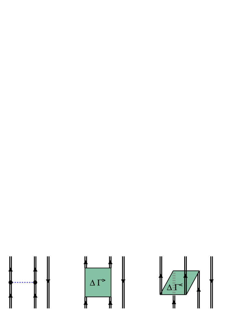
Figure 46: Diagrams that are included in the definition of the vertex for the pp channel. Here $\Delta\Gamma^{>}$ and $\Delta\Gamma^{<}$ are the forward- and backward-going part of the energy dependent contribution to the pp DRPA vertex (154a). The contribution of these three diagrams can be factorized in an expression of the form ${G^{0}}^{>}\;\Gamma^{(3)}\;{G^{0}}^{>}$ only after having redefined the propagators ${G^{0}}^{>}$ and $\Gamma^{(3)}$ to depend also on the particle and hole fragmentation indices ($n$,$n^{\prime}$,$k$).

The remaining complication, related to the use of dressed propagators, concerns the interactions vertices (153). In order to keep track of which quasiparticle or quasihole is coupled to the DRPA phonons, the $\Gamma^{(i)}$ and the propagators $R^{(i)}$ need to be redefined in such a way that their matrix elements also depend on the indices ($n$, $n^{\prime}$, $k$), which label the fragments of the sp propagator, Eq. (3). This implies that the eigenvalue equations will involve summations on both the sp indices ($\alpha$, $\beta$, $\gamma$) and the ones corresponding to the fragmentation, ($n_{\alpha}$, $n_{\beta}$, $k_{\gamma}$). The particular expression to be employed for the vertices $\Gamma^{(i)}$ depends on the approximation chosen for the pp and ph phonons and it can be crucial to control spurious solutions in the Faddeev equations. Here we only note that the diagrams of Fig. 46 are those required for the DRPA, as discussed in Ref. [32]. The 2p1h propagator and its Faddeev components, as defined in Eqs. (150), are recovered only at the end by summing the solutions over all values of ($n_{\alpha}$, $n_{\beta}$, $k_{\gamma}$) and ($n_{\mu}$, $n_{\nu}$, $k_{\lambda}$).

Putting together all the above considerations, the resulting approximation to the Faddeev equations (152) can be rewritten in a way where all the propagators involved depend only on one energy variable (or two time variables). The forward-going part of this expansion can be written as follows (after Fourier transformation to the energy representation)

$$R^{(i)}_{\mu n_{\mu}\nu n_{\nu}\lambda k_{\lambda},\alpha n_{\alpha}\beta n_{\beta}\gamma k_{\gamma}}(\omega)$$ (155)

$$= \frac{1}{2}\left({G^{0}}^{>}_{\mu n_{\mu}\nu n_{\nu}\lambda k_{\lambda},\alpha n_{\alpha}\beta n_{\beta}\gamma k_{\gamma}}(\omega)-{G^{0}}^{>}_{\nu n_{\nu}\mu n_{\mu}\lambda k_{\lambda},\alpha n_{\alpha}\beta n_{\beta}\gamma k_{\gamma}}(\omega)\right)$$

$$+~{}{G^{0}}^{>}_{\nu n_{\nu}\mu n_{\mu}\lambda k_{\lambda},\mu^{\prime}n_{\mu}^{\prime}\nu^{\prime}n_{\nu}^{\prime}\lambda^{\prime}k_{\lambda}^{\prime}}(\omega)~{}\Gamma^{(i)}_{\nu^{\prime}n_{\nu}^{\prime}\mu^{\prime}n_{\mu}^{\prime}\lambda^{\prime}k_{\lambda}^{\prime},\mu^{\prime\prime}n_{\mu}^{\prime\prime}\nu^{\prime\prime}n_{\nu}^{\prime\prime}\lambda^{\prime\prime}k_{\lambda}^{\prime\prime}}(\omega)~{}$$

$$~{}~{}~{}~{}\times~{}\left(R^{(j)}_{\mu^{\prime\prime}n_{\mu}^{\prime\prime}\nu^{\prime\prime}n_{\nu}^{\prime\prime}\lambda^{\prime\prime}k_{\lambda}^{\prime\prime},\alpha n_{\alpha}\beta n_{\beta}\gamma k_{\gamma}}(\omega)~{}+~{}R^{(k)}_{\mu^{\prime\prime}n_{\mu}^{\prime\prime}\nu^{\prime\prime}n_{\nu}^{\prime\prime}\lambda^{\prime\prime}k_{\lambda}^{\prime\prime},\alpha n_{\alpha}\beta n_{\beta}\gamma k_{\gamma}}(\omega)\right)\;,~{}~{}i=1,2,3~{}.$$

In Eq. (155), ${G^{0}}^{>}$ is the forward-going part of the 2p1h propagator for three dressed but noninteracting lines. This quantity is therefore defined as follows (without implicit summation):

$${G^{0}}^{>}_{\mu n_{\mu}\nu n_{\nu}\lambda k_{\lambda},\alpha n_{\alpha}\beta n_{\beta}\gamma k_{\gamma}}(\omega)~{}=~{}\delta_{n_{\mu},n_{\alpha}}\;\delta_{n_{\nu},n_{\beta}}\;\delta_{k_{\lambda},k_{\gamma}}$$ (156)

$$\times\frac{\langle\Psi^{A}_{0}|c_{\mu}|\Psi^{A+1}_{n_{\mu}}\rangle\langle\Psi^{A}_{0}|c_{\nu}|\Psi^{A+1}_{n_{\nu}}\rangle\langle\Psi^{A}_{0}|c^{{\dagger}}_{\lambda}|\Psi^{A-1}_{k_{\lambda}}\rangle\;\langle\Psi^{A+1}_{n_{\alpha}}|c^{{\dagger}}_{\alpha}|\Psi^{A}_{0}\rangle\langle\Psi^{A+1}_{n_{\beta}}|c^{{\dagger}}_{\beta}|\Psi^{A}_{0}\rangle\langle\Psi^{A-1}_{k_{\gamma}}|c_{\gamma}|\Psi^{A}_{0}\rangle}{\omega-(\varepsilon^{+}_{n_{\alpha}}+\varepsilon^{+}_{n_{\beta}}-\varepsilon^{-}_{k\gamma})+i\eta}\;.$$

A completely analogous set of equations apply for the backward-going (2h1p) expansion of $R(\omega)$.

Equations (155) reduce the general “Faddeev-Bethe-Salpeter” expansion, Eq. (152), to a tractable set of equations involving only two-time objects. It is important to note that these equations are still expressed in terms of the self-consistent solution $g_{\alpha\beta}(\omega)$ and include both the collective pp and ph phonons in a correct way. Thus they maintain all the features relevant for the physics that have been discussed at the beginning of this subsection.

5.5 Single-particle spectral function of ${}^{16}{\rm O}$

A self-consistent solution of the spectral function of ${}^{16}{\rm O}$ was obtained in Ref. [197] by solving the set of Faddeev equations (155). The Dyson equation was solved within a model space consisting of harmonic oscillator sp states. An oscillator parameter $b=$ 1.76 fm was chosen (corresponding to $\hbar\omega=$ 13.4 MeV) and all the first four major shells (from $1s$ to $2p1f$) plus the $1g_{9/2}$ where included. Inside this model space, the interaction used was a Brueckner $G$-matrix [223] derived from the Bonn-C potential [207]. For the solution of the Faddeev equations a $G$-matrix evaluated at a fixed starting energy $\omega=$-25 MeV was chosen as a suitable average of the energy the most important 2h1p states that couple to the experimentally observed quasiholes [199]. However, the energy dependence of $G(\omega)$ was taken into account in the calculation of the mean field part of the self-energy, resulting in the Brueckner-Hartree-Fock approximation (this can be compared to the HF case in Eq. (18) ),

$$\Sigma^{BHF}_{\alpha\beta}(\omega)=i\sum_{\gamma\delta}\int\frac{d\omega^{\prime}}{2\pi}G_{\alpha\gamma,\delta\beta}(\omega+\omega^{\prime})g_{\gamma\delta}(\omega^{\prime})$$ (157)

The self-energy was then computed as in Eq. (19), with Eq. (157) instead of $\Sigma^{HF}$.

The normalization (spectroscopic factor) of each sp fragment was computed by means of Eq. (38), which we rewrite here in the form

$$Z_{k}=\sum_{\alpha}\left|{\cal Y}^{k}_{\alpha}\right|^{2}=1+\sum_{\alpha,\beta}\left({\cal Y}^{k}_{\alpha}\right)^{*}\left.\frac{\partial\Sigma^{\star}_{\alpha\beta}(\omega)}{\partial\omega}\right|_{\omega=\varepsilon^{-}_{k}}{\cal Y}^{k}_{\beta}\;\;.$$ (158)

where ${\cal Y}^{k}_{\alpha}\sim{\mbox{$\langle{\Psi^{A-1}_{k}}|$}}c_{\alpha}{\mbox{$|{\Psi^{A}_{0}}\rangle$}}$ represent the $k$-th solution for the spectrocopic amlitudes and $\varepsilon^{-}_{k}\sim E^{A}_{0}-E^{A-1}_{k}$ the corresponding eigenvalue. It is important to note that the $\Sigma^{BHF}(\omega)$ component of the self-energy also contributes to reduction the spectroscopic factor. This energy dependence, associated with the use of the $G$-matrix in Eq. (157), is not present in a standard HF self-energy and originates from the states at high energy that are excluded from the model space. In Ref. [196], it was found that this procedure properly accounts for the depletion of spectroscopic factors that is induced by SRC, at least for the normally occupied shells in the IPM.

The solution of RPA equations may lead to collective instabilities whenever interactions are employed that are too attractive. A particular sensitivity to the strength of the $G$-matrix interaction was found in the calculation of [197, 200], only for the lowest isoscalar $0^{+}$ solution. For this reason an artificial shift of its eigenvalue to the experimental energy of first excited state, 6.049 MeV, was maintained during the successive iterations. Note that the screening due the redistribution of the sp strength tends to reduce the instability problem in DRPA. Moreover, the origin of the instability for this particular solution has been identified and corrected later, in Ref. [200].

Shell		TDA		RPA		1st itr.		2nd itr.		3rd itr.		4th itr.
$Z_{p_{1/2}}$		0.775		0.745		0.775		0.777		0.774		0.776
$Z_{p_{3/2}}$		0.766		0.725		0.725		0.727		0.722		0.724
						0.015		0.027		0.026		0.026
Total occ.		14.56		14.56		14.56		14.57		14.58		14.63

Table 3: Hole spectroscopic factors ($Z_{\alpha}$) for knockout of a $\ell=1$ proton from ${}^{16}{\rm O}$. These results refer to the initial IPM calculation in TDA and RPA and to the first four iterations of the DRPA equations. All the values are given as a fraction of the corresponding IPM value. Also included is the total number of nucleons, as deduced from the complete one-hole spectral function, for each iteration.

The Faddeev equations were solved first in terms of a IPM input propagator in both TDA and RPA approximations. For an IPM ansatz, the TDA calculation is equivalent to the one of Ref. [196] and yields the same results for the spectroscopic factors of the main particle and hole shells close to the Fermi energy. These correspond to 0.775 for $p_{1/2}$ and 0.766 for $p_{3/2}$ as reported in Tab. 3. The introduction of correlations reduces these values and brings them down to 0.745 and 0.725, respectively. This result reduces the discrepancy with the experiment by about 4% and shows that collectivity beyond the TDA level is relevant to explain the quenching of spectroscopic factors. Since the present formalism does not account for center-of-mass effects, the above quantities need to be increased by about 7% before they are compared with the experiment [24, 198].

The RPA results have been iterated several times, with the aim of studying the effects of fragmentation on the RPA phonons and, subsequently, on the spectral strength. Since one is mainly interested in the low-energy excitations, it is sufficient to keep track only of the strongest fragments that appear —close to the Fermi energy— in the (dressed) sp propagator, Eq. (3), while the residual strength is collected in two effective poles, above and below the Fermi level, for each orbital [193, 197]. As shown in Tab. 3, only a few iterations are required to reach convergence for the values of the spectroscopic factors. The converged distribution of one-hole strength is compared with the experimental one in Fig. 47. The main difference between these results and the one obtained by using an IPM input is the appearance of a second smaller $p_{3/2}$ fragment at -26.3 MeV. This peak arises in the first two iterations and appears to become stable in the last one, with a spectroscopic factor of 2.6%. This can be interpreted as a peak that describes the fragments seen experimentally at slightly higher energy. This result corresponds to the first time that such a fragment is obtained in calculations of the spectral strength.

A second effect of including fragmentation in the construction of the RPA phonons is to increase the strength of the main hole peaks. The $p_{1/2}$ strength increases from the 0.745 obtained with IPM input to 0.776, essentially canceling the “improvement” gained by the introduction of RPA correlations over the TDA ones. The main peak of the $p_{3/2}$ remains at 0.722 but the appearance of the secondary fragment slightly increases the overall strength for this orbital as well. This behavior is due to the fact that redistribution of the strength (and principally, the reduction of the main spectroscopic factors) tends to screen the nuclear interaction, with respect to the IPM case. The consequence is a reduced effect of RPA correlations when fragmentation is included in the construction of the phonons. This feature has also been observed in other self-consistent calculations of the sp spectral strength, for example in nuclear matter [73]. Obviously, this makes the disagreement with experiments a little worse and additional work is needed to resolve the disagreement with the data. Nevertheless, it is clear that fragmentation is a relevant feature of nuclear systems and that it has to be properly taken into account.

Together with the main fragments, the Dyson equation produces also a large number of solutions with small spectroscopic factors. This strength extends down to about -130 MeV for the one-hole spectral function and up to about 100 MeV for the one-particle case. This background represents the strength that is removed from the main peaks and shifted up or down to medium missing energies. Another 10% of strength is moved to very high energies due to SRC [61]. Its location cannot be explicitly calculated in the present approach but the effects on the reduction of spectroscopic factors at low energy is accounted through the energy dependence of the $G$-matrix. Accordingly the total number of nucleons deduced from the fully self-consistent spectral function is 14.6 as reported in Tab. 3. This gives an estimate for the overall occupancy of high-momentum states of about 10%, in agreement with direct calculations [184, 151] as discussed in Secs. 5.2 and 5.3.

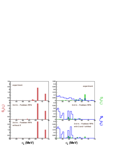
Figure 47: One-proton removal strength as a function of the hole sp energy $\varepsilon^{-}_{k}=E^{A}_{0}-E^{A-1}_{k}$ for ${}^{16}{\rm O}$ for angular momentum $\ell=1$ (left) and $\ell=0,2$ (right). For the positive parity states, the solid bars correspond to results for $d_{5/2}$ and $d_{3/2}$ orbitals, while the thick lines refer to $s_{1/2}$. The top panels show the experimental values taken from [199]. The middle panels give the theoretical results for the self-consistent spectral function. The bottom panels show the results obtained by repeating the 3^rd iteration with a modified ph-DRPA spectrum, in which the lowest eigenstates have been either removed or shifted to the corresponding experimental values.

We note that the present approach also yields predictions for the strength distribution of quasiparticle excitations. Although little experimental information is available for the addition of a nucleon (as well as for the removal of a neutron). Other knockout and nucleon transfer reactions, employing nuclear probes, have been recently been developed or reanalyzed to extract hole spectroscopic factors of both stable and radioactive nuclei [224, 225]. These tools may yield better accuracies than in the past and can, in principle, be used to extract information on the one-particle spectral distribution.

A deeper insight into the mechanisms that generate the fragmentation pattern can be gained by investigating directly the connection between the spectral function and some specific collective states. To clarify this point we repeated the third iteration using exactly the same input but without keeping the lowest ph $0^{+}$ state at its experimental energy, it was discarded instead. The resulting $p$ hole spectral function is shown in the lower-left panel of Fig. 47. In this calculation no breaking of the $p_{3/2}$ strength is obtained but only a single peak is found with a spectroscopic factor equal to 0.75, which is the sum of the two fragments that are obtained when the $0_{2}^{+}$ state is taken into account. This result can be interpreted by considering the $p_{3/2}$ fragments as a hole in the ground state and in the first excited $0^{+}$ state of the ${}^{16}{\rm O}$ core, respectively. The correct fragmentation pattern can be reproduced only when the latter two levels are close enough to one another in energy, so that the two configurations can mix.

The other two low-lying states of ${}^{16}{\rm O}$ that may be of some relevance are the isoscalar $1^{-}$ and $3^{-}$. These excitations are reproduced reasonably well by RPA type calculations [162] but are typically found at $\sim$3 MeV above the experimental results. The lower panels of Fig. 47 show the results for the even parity spectral functions that are obtained when both the $3^{-}$ and the $1^{-}$ ph-DRPA solutions are shifted to match their experimental values. In this case, a $d_{5/2}$ hole peak is obtained at a missing energy -17.7 MeV, in agreement with experiment, and with a spectroscopic strength of 0.5%. It is interesting to note that the shifting of the $3^{-}$ and $1^{-}$ collective states does not produce any other noticeable change in the theoretical spectral function.

5.6 Spectrum of ${}^{16}{\rm O}$ and extension of RPA

The above results suggest that the main impediment for further improvements of the description of the experimental spectral strength is associated with the deficiencies of the RPA (DRPA) description of the excited states. One important problem is the first excited state, with quantum numbers $0^{+}$, which is seen to produce important effects on the fragmentation of the $p$ shell. The DRPA result do find this state at low energy but can describe at most one collective phonon for a given angular momentum, parity, and isospin combination $J^{\pi},T$ whereas several low-lying isoscalar $0^{+}$ and $2^{+}$ excited states are observed at low energy in ${}^{16}{\rm O}$, as well as additional $3^{-}$ and $1^{-}$ states. A possible way to proceed would be to first concentrate on an improved description of the collective phonons by extending the RPA to explicitly include the coupling to two-particle$-$two-hole (2p2h) states. Such an extended RPA procedure has been applied in heavier nuclei with considerable success [226, 227]. In order to be relevant for ${}^{16}{\rm O}$, this approach requires an extension in which the coherence of the 2p2h states is included in the form of the presence of two-phonon excitations [228]. This corresponds to adding two-phonon configurations to the kernel $K^{ph}$ of the BSE for the ph propagator (21), as shown in Fig. 48 [200].

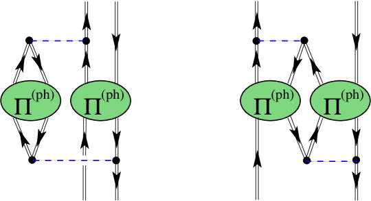
Figure 48: Examples of contributions involving the coupling of two independent ph phonons. In total, there are sixteen possible diagrams of this type, obtained by considering all the possible couplings to a ph state. The two-phonon ERPA equations sum all of these contributions in terms of dressed sp propagators.

The formalism to include two-phonon configurations has been presented in Ref. [200], where it is referred as two-phonon extended RPA (ERPA). In that work the ph-DRPA equation has been solved first, using the self-consistent sp propagator discussed in Sec. 5.5. The lowest DRPA solutions for both the $0^{+}$, $3^{-}$ and $1^{-}$ channels were shifted down to their respective experimental energies and then employed to generate the two-phonon contributions for the ERPA calculation. The spectrum obtained for ${}^{16}{\rm O}$ is displayed in Fig. 49 and Tab. 4 together the total ph strength $Z_{n_{\pi}}$ of each state,

$$Z_{n_{\pi}}~{}=~{}\sum_{\alpha\beta}~{}\left|{\mbox{$\langle{\Psi^{A}_{n_{\pi}}}|$}}c^{{\dagger}}_{\alpha}c_{\beta}{\mbox{$|{\Psi^{A}_{0}}\rangle$}}\right|^{2}\;.$$ (159)

Tab. 4 also reports the relative strength of ph and two-phonon admixtures in the wave function for each solution of the ERPA equation. Due to the screening effects associated with dressing the sp propagators, the solution for the first isoscalar $0^{+}$ state in DRPA is found much higher in energy at $\sim$17 MeV. It is important to realize that this solution has a sharp ph character and therefore it cannot be identified with the experimental $0_{2}^{+}$ state. The latter state is known to be dominated by 4$\hbar\omega$ configurations [230, 231, 216]. On the other hand inelastic electron scattering experiments [232] clearly excite this state. From the point of view of the SCGF approach, the one-body response is completely described by the polarization propagator, Eq. (23), and therefore, the total one-body strength must be represented by $Z_{n_{\pi}}$ (159). This indicates a strong coupling to the (dressed) ph propagator (23). On the basis of this similarity, it still seems plausible to shift the ph-DRPA solution down in energy in order to study its mixing with other configurations.

The corresponding results yield an isoscalar $0^{+}$ state with a predominant ph character at $\sim$17 MeV, as it was found in DRPA. Although this solution is now characterized by a partial mixing with two-phonon configurations. Tab. 4 shows that this is the result of mixing with the lowest solution in the same channel, which ends up at $\sim$11 MeV. The latter is predominately a two-phonon state. It is also seen that in both cases the relevant configuration comes from the coupling of two $0^{+}$ phonons themselves. in Ref. [200] it was found that the wave functions for these two states contain several relevant ph configurations, obtained from different quasiparticle fragments in the $pf$ ($sd$) shells combined with quasihole fragments of the $p$ ($s$) shells. Therefore, the situation is more complicated than the simple picture of only two levels interacting with each other.

The calculations of Ref. [233] have shown that the bulk of the 4p4h contributions to the first excited state of ${}^{16}\textrm{O}$ may come from the coupling of four different phonons with negative parity ($3^{-}$ and $1^{-}$). However, the self-consistent role of coupling positive parity states was not considered in that work. Both this effect, the RPA correlations and the inclusion of the nuclear fragmentation allow for the –at least partial– inclusion of configurations beyond the 2p2h case even when no more than two-phonon coupling is considered, as discussed here. Still it would be helpful to further study the importance of three- and four-phonon configurations within this apporach.

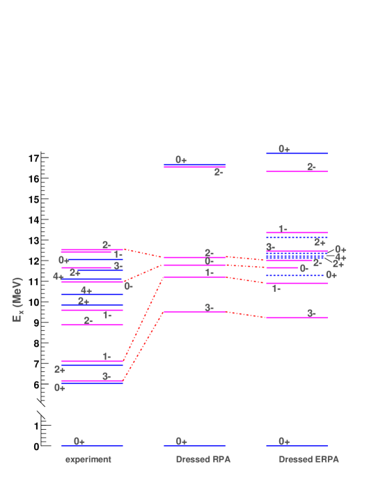
Figure 49: Results for the DRPA and the two-phonon ERPA propagator of ${}^{16}\textrm{O}$ with the dressed input propagator computed in Ref. [197], middle and last column respectively. In solving the ERPA equation, the lowest $3^{-}$, $1^{-}$ and $0^{+}$ levels of the DRPA propagator where shifted to their experimental energies. All other DRPA solutions were left unchanged. The excited states indicated by dashed lines are those for which the (E)RPA equation predicts a total spectral strength $Z_{n_{\pi}}$ lower than 10%. The first column reports the experimental results [229].

The low-lying negative parity isoscalar states ($3^{-}$ and $1^{-}$) are only slightly affected by two-phonon contributions and remain substantially above the experimental energy at 9.23 and 10.90 MeV, respectively, and more correlations will be needed in order to lower their energy. We note that these wave functions contain a two-phonon admixture obtained by coupling the low-lying $0^{+}$ excitation to either the $3^{-}$ or $1^{-}$ phonons. According to the above interpretation of the first $0^{+}$ excited state this corresponds to the inclusion of 3p3h and beyond. At the same time two additional negative parity solutions, with two-phonon character, are found at higher energy in accordance with experiment. These configurations are not reproduced by the simple DRPA.

$T=0$		dressed/DRPA			dressed/ERPA						$(0_{2}^{+})^{2}$	$(3_{1}^{-})^{2}$	$(0_{2}^{+},3_{1}^{-})$	$(0_{2}^{+},1_{1}^{-})$
$J^{\pi}$		$\varepsilon^{\pi}_{n}$	$Z_{n_{\pi}}$		$\varepsilon^{\pi}_{n}$	$Z_{n_{\pi}}$		$ph$(%)	$2\Pi$(%)		(%)	(%)	(%)	(%)
$1^{-}$					13.37	0.148		21	79					79
$3^{-}$					12.35	0.113		16	84				84
$0^{+}$					12.15	0.001		1	99		3	96
$4^{+}$					12.14	0.007		1	99			99
$2^{+}$					12.12	0.008		1	99			98
$0^{+}$		16.62	0.717		17.21	0.633		88	12		10	0.5
$0^{+}$					11.28	0.092		12	88		85	2
$1^{-}$		11.19	0.720		10.90	0.680		94.1	5.9					5.8
$3^{-}$		9.50	0.762		9.23	0.735		95.9	4.1				4.0

Table 4: Excitation energy and total spectral strengths obtained for the principal solutions of DRPA and two-phonon ERPA equations. The total contribution of ph and two-phonon states of the ERPA solutions are shown. For states below 15 MeV, the columns on the right side give the individual contributions of all the relevant two-phonon contributions.

The two-phonon ERPA approach also generates a triplet of states at about 12 MeV, with quantum numbers $0^{+}$, $2^{+}$ and $4^{+}$. A similar triplet is found experimentally at 12.05, 11.52 and 11.10 MeV, which also corresponds to twice the experimental energy of the first $3^{-}$ phonon. The ERPA solutions for this triplet are almost exclusively obtained by $3^{-}\otimes 3^{-}$ states and therefore have a 2p2h character, in accordance with Refs. [232, 235, 236]. Further interaction in the pp and hh channels will be needed in order to reproduce the correct experimental splitting and experimental strength [233, 234].

5.7 Results for the ${}^{16}{\rm O}(e,e^{\prime}pp)$ cross section

Data from two-nucleon knockout reactions have been measured recently at NIKHEF [52, 237, 238, 239] and MAMI [240, 241] facilities for different targets. Theoretically, these cross sections can be computed with the models developed by the Pavia [242, 243] and Ghent [244] groups for the emission of both two protons or a proton-neutron pair. Calculation for the ${}^{16}{\rm O}(e,e^{\prime}pp)$ case have shown that the transition to the ground state of ${}^{14}{\rm C}$ is dominated by the high-momentum components in the two-nucleon overlap function. Comparison with the data from NIKHEF for this reaction have provided a clear signature of SRC effects [238, 245].

An important ingredient in the description of two-nucleon knockout reactions is the two-hole spectral function. This quantity can be extracted from the imaginary part of the two-body propagator $g^{II}(\omega)$, compare Eqs. (27) and (54), and contains the nuclear structure information on the correlated pair before the reaction takes place. The propagator $g^{II}(\omega)$ can be obtained by solving pp(hh) RPA equations as done in Ref. [246]. However, typical calculations of this kind yield results within a model space that is too small to contain the short-range effects. In these cases one needs to compute the high-momentum components separately. In the following we outline the approach taken in Refs. [246, 242] and show a few results for the ${}^{16}{\rm O}(e,e^{\prime}pp)$ cross section.

The sp spectral function of ${}^{16}{\rm O}$ obtained in Ref. [196] was employed as the starting point of a hhDRPA calculation (see Eq. (29) ), eventually obtaining a two-hole spectral function of the form [246],

$$S^{hh}_{JT}({\bf p}_{1},{\bf p}_{2},{\bf p}_{1^{\prime}},{\bf p}_{2^{\prime}},\omega)=$$ (160)

$$\sum_{k}\sum_{abcd\in{\cal P}}\sum_{MT_{3}}\Phi^{\ast JM}_{cd}({\bf p}_{1^{\prime}},{\bf p}_{2^{\prime}})\left(X^{k}_{cdJT}\right)^{*}X^{k}_{abJT}\Phi^{JM}_{ab}({\bf p}_{1},{\bf p}_{2})\;\delta(\omega-(E^{A}_{0}-E^{JT,A-2}_{k}))\;,$$

where $J$ and $T$ refer to the total angular momentum and isospin of the residual nucleus and $M$ and$T_{3}$ are their projections. In Eq. (160), the energies $E^{JT,A-2}_{k}$ are the the DRPA solutions for excitation energies of the residual nucleus and the quantities

$$X^{k}_{abJT}\sim\langle\Psi^{k,A-2}_{J}||\tilde{(a_{\beta}a_{\alpha})}_{J}||\Psi^{A}_{0}\rangle$$ (161)

represent the components of the solutions for the two-body overlap amplitudes. The sums extend only over those orbitals that are occupied in the model space ${\cal P}$ and the spectral function $S^{hh}(\omega)$ is transformed into the momentum representation by employing two-body harmonic oscillator wave functions $\Phi^{JM}_{ab}({\bf p}_{1},{\bf p}_{2})$.

The description of the high-momentum components due to SRC requires the inclusion of a very large number of basis states, at least up to $100\hbar\omega$ in a harmonic oscillator basis [223]. However, the description of long-range correlations by solving a Bethe-Salpeter or an RPA equation (29) is not feasible within such a large space. For this reason the complete basis is split into a model space ${\cal P}$, and a complementary space ${\cal Q}={\bf 1}-{\cal P}$. For ¹⁶O the space ${\cal P}$ was chosen to contain the orbitals up to the $pf$ shell only, which is large enough to accommodate long-range effects. The justification for this procedure is that SRC are caused by close encounters of two nucleons, which mainly depend on the nuclear density and therefore are not very sensitive to details of the long-range structure. The latter, on the other hand, may be calculated within the space ${\cal P}$ with a suitable effective interaction in which the SRC are incorporated at least in ladder approximation. This effective interaction can then be obtained by following Brueckner’s individual pair approach [247, 248] by solving the Bethe-Goldstone equation (BGE). Using the technique of Ref. [223] the equation for the correlated pair wave function

$$|\Psi_{ab}\rangle=|\Phi_{ab}\rangle+\frac{\hat{Q}}{\omega-\hat{H}_{0}}\hat{V}|\Psi_{ab}\rangle\;,$$ (162)

is solved in the finite nucleus. In this equation the Pauli operator $\hat{Q}$ prohibits scattering into orbits of the finite shell-model space ${\cal P}$, in which long-range correlations are trated in an DRPA approach. In Eq. (162), $\Phi_{ab}$ represents the same uncorrelated shell model wave functions appearing in Eq. (160), $\omega$ is the propagation energy of the pair and $\hat{H}_{0}$ is the Hamiltonian without residual interaction. In this case, the energy $\omega$ refers to the propagation of two holes which precludes the vanishing of the denominator in Eq. (162).

From the solution of Eq. (162) one obtains the defect wave function as the difference between the correlated and uncorrelated pair wave functions

$$|\chi\rangle=|\Psi\rangle-|\Phi\rangle\;,$$ (163)

which represent the components of the two-body wave function that are orthogonal to the space ${\cal P}$, and the $G$ matrix as the effective interaction in ${\cal P}$ according to

$$\langle\Phi^{JM}_{cd}|G|\Phi^{JM}_{ab}\rangle=\langle\Phi^{JM}_{cd}|V|\Psi^{JM}_{ab}\rangle\;.$$ (164)

The essential step taken here, is to approximate the spectral function (160) by the expression

$$S^{hh}_{JT}({\bf p}_{1},{\bf p}_{2},{\bf p}_{1^{\prime}},{\bf p}_{2^{\prime}},\omega)=$$ (165)

$$\sum_{k}\sum_{abcd\in{\cal P}}\sum_{MT_{3}}\Psi^{*\;JM}_{cd}({\bf p}_{1^{\prime}},{\bf p}_{2^{\prime}})\left(X^{k}_{cdJT}\right)^{*}X^{k}_{abJT}\Psi^{JM}_{ab}({\bf p}_{1},{\bf p}_{2})\;\delta(\omega-(E^{A}_{0}-E^{JT,A-2}_{k}))\;,$$

where the summation over orbits is still limited to the finite shell-model space ${\cal P}$ but the uncorrelated wave functions are replaced by the correlated ones (see Eq. (162) ). This is in line with the argument just given, that hard binary collisions, treated in the BGE and giving rise to high-momentum components, proceed independently of the long-range correlations. The latter are taken into account in the shell model amplitudes $X$ within the limited space ${\cal P}$.

Figure 50: Superposition of spectral functions (55) appropriate for the removal of two protons with final momenta ${\bf p}_{1}$ and ${\bf p}_{2}$ from ¹⁶O leading to the final $0^{+}$ ground state or first excited $2^{+}$ state in ¹⁴C. The plots are given for a kinematic setting used in experiments at NIKHEF [237]. The momentum vector ${\bf q}$ is fixed along the $z$-axis, with length $313$ MeV/c. The momenta ${\bf p}_{1}$ and ${\bf p}_{2}$ are in the same plane with ${\bf q}$ at $-49$ and $123$ degrees angles with respect to this transferred momentum, respectively. The upper plots correspond to harmonic oscillator wave functions without the inclusion of short-range correlations (see Eq. (160) ). In the lower plots these SRC are incorporated by the defect functions computed the Reid and the Bonn-A potential (Eqs. (163) and (165) ).

In the spectator model with a plane-wave approximation for the outgoing protons, the contribution of the spectral function to the cross section is given by the superposition $\hat{S}(\bm{p}_{1},\bm{p}_{2},E)$, Eq. (55). This function is plotted in Fig. 50, at the kinematics corresponding to the ${}^{16}{\rm O}(e,e^{\prime}pp)$ measurements at NIKHEF [237], for the transitions to the $0^{+}$ ground state and to the excited $2^{+}$ levels of ${}^{14}{\rm C}$. In these kinematics the momenta $\bm{p}_{1}$ and $\bm{p}_{2}$ of the protons are almost antiparallel to each other and coplanar with the momentum $\bm{q}$ transferred by the electron. As a consequence, high and equal values of their magnitudes correspond to high relative momenta in the plots of Fig. 50. The effects of including the SRC is shown in the lower plots, where the correlation functions (163) have been computed with both the Reid-Soft-Core and Bonn-A potentials. Figure 50, also shows the plots labeled ‘No SRC’ that correspond to neglecting the correlation functions and computing the spectral functions with Eq. (160). As expected, one observes that the latter gives no contribution at higher momenta. The high-momentum part of the spectral function is about a factor of two larger for the Reid-Soft-Core potential than for the Bonn-A potential in the momentum range around $3$–$5$ fm^-1. The short-range correlations give rise to a spectral function which is clearly distinct from the one without SRC.

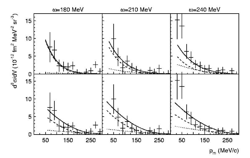
Figure 51: The cross sections for the transition to the ground state in ${}^{14}{\rm C}$ as a function of the missing momentum, measured for the reaction ${}^{16}{\rm O}(e,e^{\prime}pp){}^{14}{\rm C}$ at three values of $\omega$. The curves are obtained from calculations of Refs. [242] (top) and [244] (bottom). The solid curves represent the calculated cross sections; the dashed and dotted curves correspond to the contributions of the one- and two-body hadronic currents, respectively.

The Ghent-model [244] accounts for SRC in a different way. There, single-particle wave functions obtained from Hartree-Fock calculations are used and the many-body wave function, is approximated to first order in the correlation function,

$$\Psi({\bf r}_{1},\ldots{\bf r}_{A})=\prod^{A}_{i<j=1}\left(1-g(r_{ij})\right)\Phi({\bf r}_{1},\ldots{\bf r}_{A})/\sqrt{N}\;,$$ (166)

where $N$ is a normalisation factor. The effects of SRC are included in the factor $(1-g(r_{ij}))$ by means of the correlation function $g(r_{ij})$ (which zero in the absence of correlations). The calculations presented here employed the $g(r_{ij})$ of Ref. [65], also shown in Fig. 29.

Figure 51 compares the cross sections for the calulations of Ref. [242, 244] with the experimental data, as a function of the missing momentum at the three values of $\omega$ [245]. For this calculation final state interactions for the outgoing protons were taken into account by using distorted waves but neglecting their mutual interaction. A pair of $(p_{1/2})^{2}$ or $(p_{3/2})^{2}$ protons can be coupled to total angular momentum $J$=0, leaving the ${}^{14}{\rm C}$ nucleus in the ground state, through either a ${}^{1}S_{0}$ or a ${}^{3}P_{1}$ relative state. The coupling scheme used in the calculation is as follows. The ${}^{1}S_{0}$ state is always associated with an angular momentum of the center-of-mass motion $L=0$, and the ${}^{3}P_{1}$ state always with $L=1$. From Fig. 51 it is clear that for all three values of the energy the missing-momentum dependence of the measured cross sections is similar. In Refs. [237, 238], it has been pointed out that such a momentum distribution reflects an angular momentum $L=0$ for the center-of-mass motion of the pair, and thus suggests a dominant role for the knockout of a ${}^{1}S_{0}$ pair driven by SRC. The theoretical cross sections are represented in Fig. 51 by the solid curves; the contributions of the one- and two-body currents are given by the dashed and dotted curves, respectively. The calculated cross sections agree well with the data at all three values of $\omega$. The curves, representing the contributions of the one- and two-body currents to the ground-state transition, indicate that at $\omega$=180 and 210 MeV the reaction is dominated by one-body currents, and that the contribution of two-body currents increases with increasing energy transfer. Conceptually both models are quite similar, and neither of the two contains free parameters. The effects due to SRC, though, are accounted for in different ways as discussed above. The Bonn-A and Reid Soft Core potentials, adopted in the calculations, are both realistic NN-potentials and successfully used in many nuclear-structure calculations. Hence, the data agree with the theoretical results obtained independently with the two models. Furthermore, both models predict that the largest contribution to the cross section stems from one-body hadronic currents driven by SRC. This justifies the conclusion that evidence is obtained for SRC although the data do not distinguish details of the actual form of the SRC. Future experiments will include the removal of proton-neutron pairs and therefore may also yield information on tensor correlations  [243, 249]. An improved description of the mutual interaction between the outgoing protons [250, 251] will help in further developing the usefulness of this reaction to elucidate details of short-range nuclear dynamics.

5.8 Extraction of spectroscopic information from $(e,e^{\prime}p)$ reactions at high ${\cal Q}^{2}$

The analysis of the (e,e^′p) data has relied on the Distorted Wave Impulse Approximation (DWIA) for both the Coulomb distortion of the electron waves (in heavy nuclei) and the outgoing proton [11, 17, 252, 253]. Some aspects of this analysis have been discussed in Sec. 3. The proton distortion is described in terms of an optical potential required to describe elastic proton scattering data at relevant energies [15]. There is some uncertainty related to this treatment since elastic proton scattering is considered to be a surface reaction and no detailed information is obtained related to the interior of the nucleus. This uncertainty gives rise to an estimated error of about 10%. Such an estimate may be inferred by considering the difference between the relativistic and nonrelativistic treatment of the proton distortion. It is shown in Ref. [254] that this difference is essentially due to the reduction of the interior wave function in the relativistic case. This feature can also be generated by including a reasonable amount of nonlocality in the optical potential [254].

A serious challenge to the interpretation of (e,e^′p) experiments was recently published in Refs. [255, 256]. This challenge consists in questioning the validity of the constancy of the spectroscopic factor as a function of the four-momentum (squared), $Q^{2}$, transferred by the virtual photon to the knocked-out nucleon. In Ref. [255] a conventional analysis of the world’s data for (e,e^′p) experiments on ${}^{12}{\rm C}$ at low $Q^{2}$ generated results consistent with previous expectations. Data at higher values of $Q^{2}$ were then analyzed within the framework of a theoretical model which employs Skyrme-Hartree-Fock bound-state wave functions for the initial proton, a Glauber-type description of the final-state interaction of the outgoing proton, and a factorization approximation for the electromagnetic vertex [255, 256]. Within the framework of this theoretical description, spectroscopic factors were obtained which increase substantially with increasing $Q^{2}$ for the ${}^{12}{\rm C}$ nucleus.

The spectroscopic factor defined in Sec. 2 is a many-body quantity defined without reference to a probe. The discussion in Sec. 3 shows that this spectroscopic factor is obtained by comparing a calculation of the cross section with the actual data. The wave function of the removed nucleon is the solution of a Woods-Saxon potential at the appropriate removal energy. This potential is adjusted to generate an optimum description of the shape of the experimental cross section. This resulting theoretical representation of the cross section is then multiplied by a constant factor to coincide with the experimental cross section. This constant factor is then interpreted as the spectroscopic factor. Another important ingredient in this analysis is the choice of the electron-proton cross section which must be considered off-shell [257]. This leads to a small additional uncertainty in the analysis of low $Q^{2}$ data as discussed recently in Ref. [258].

Further clarification of this intriguing situation with different spectroscopic factors at different $Q^{2}$ has been obtained in Ref. [259]. In this paper a study of recently published (e,e^′p) data for ${}^{16}{\rm O}$ at $Q^{2}=0.8$ (GeV/$c)^{2}$ [260] has been presented. An unfactorized approach was used, as it is required at low $Q^{2}$ [17] and as it has been recently advocated also for high $Q^{2}$ reactions in Ref. [261]. However, the higher energy of the outgoing proton requires a description which contains different elements than the conventional low $Q^{2}$ analysis. For the electromagnetic current operator the approach of Ref. [262] was followed, where a relativistic current operator was used in a Schrödinger-based calculation, avoiding any nonrelativistic reduction and including the effect of spinor distortion by the Dirac scalar and vector potentials. As for the final state, a recently developed eikonal description of the final-state interaction (FSI) of the proton with the nucleus that has been tested against DWIA solutions of a complex spin-dependent optical potential [263, 264] was employed. The absorption of the proton was described theoretically by linking it to the corresponding absorption of a nucleon propagating through nuclear matter. The relevant quantity is the nucleon self-energy which is obtained from SCGF calculations of nucleon spectral functions discussed in Sec. 4.6. This description of FSI was combined with previous results for the bound-state wave functions of the $p$-shell quasihole states in ${}^{16}{\rm O}$ [151] discussed in Sec. 5.2. In Ref. [210] these wave functions have been used to analyze low $Q^{2}$ data for the ¹⁶O(e,e^′p) reaction [199]. These very same wave functions produce a good description of the shape of the coincidence cross section for the $p$-shell quasihole states at high $Q^{2}$ [260] using the same spectroscopic factors obtained from the low $Q^{2}$ data [199].

We first establish the quality of the original assertion pertaining to low $Q^{2}$ by referring to Fig. 42 for the $p3/2$ state in ¹⁶O. A similar result is obtained for the $p1/2$ state [259]. The corresponding spectroscopic factors to obtain agreement with these low $Q^{2}$ data are given by 0.644 and 0.537 for the $p1/2$ and $p3/2$ states, respectively. In Fig. 52 the same reaction is considered in a very different kinematical regime, namely at constant $(\bm{q},\omega)$ with $Q^{2}=0.8$ (GeV$/c)^{2}$ [260]. The data here refer to a five-fold differential cross section, avoiding any ambiguity in modelling the half off-shell elementary cross section $\sigma_{ep}$. Results for the transition to the ground state $p_{1/2}$ have been multiplied by 20.

Figure 52: Cross section for the ¹⁶O(e,e^′p)¹⁵N reaction at $Q^{2}=0.8$ (GeV/$c)^{2}$ in perpendicular kinematics [260]. Data for the $p1/2$ state have been multiplied by 20. The solid lines represent the result of the calculation [259]. The dashed lines are obtained by replacing the quasihole states with the bound state wave functions of Ref. [265]. In all cases, the results have been rescaled by the same spectroscopic factors as used for the NIKHEF kinematics (see Fig. 42 for example), namely Z=0.644 and Z=0.537 for the $p1/2$ and $p3/2$ states, respectively.

The theoretical calculations are displayed with solid lines for the results with the quasihole bound state and dashed lines by employing the wave function of Ref. [265]. The preference for the first choice is evident. In any case, it is remarkable that the calculations reproduce the data by using the same spectroscopic factors as in the previous kinematics, i.e. $Z_{0p1/2}=0.644$ and $Z_{0p3/2}=0.537$. Therefore, contrary to the findings of Ref. [256], no need for a $Q^{2}$ dependence of the spectroscopic factors over a wide kinematical range has been established. This is also in agreement with the results obtained by a mean-field description in the context of relativistic DWIA [266]. This outcome is reassuring and is further confirmed in Ref. [267]. In this paper it is also shown that a similar statement holds when the analysis of the data is performed using a relativistic description of the distorted proton waves combined with a corresponding mf description of the bound states. Also in this case, the slightly larger spectroscopic factors of 0.708 and 0.602 for the $p1/2$ and $p3/2$, respectively describe both the low and high $Q^{2}$ data. The difference between the spectroscopic factors for these different analyses is about 5% which may be considered as a measure of the uncertainties associated with the assignment of spectroscopic factors until an improved microscopic desciption of the FSI becomes available.

Finally, one may conclude that the treatment of the bound-state wave function is not responsible for the $Q^{2}$ dependence found in Ref. [256]. From this observation one may infer that it is useful to extend the analysis of the high $Q^{2}$ data to other nuclei using the eikonal description supplemented with the nuclear matter damping description while foregoing the use of microscopic quasihole wave functions. Clearly an analysis of the data considered in Refs. [255] and [256] will further clarify the validity of the present analysis. It is already encouraging to note that the damping employed in the calculations is adequate to describe the observed absorption in the NE18 experiment [268] as discussed in Ref. [259].

5.9 Recent experimental data at higher missing energies

The bulk of experimental data obtained during the last decades by means of the (e,e^′p) reaction have focussed almost exclusively on the shells in the immediate vicinity of the Fermi energy, especially for heavier nuclei. As a consequence the amount of protons seen experimentally has been considerably smaller than the total number of protons $Z$ inside the nucleus.

Figure 53: Experimental occupation number for the all the mean field shells of ${}^{208}{\rm Pb}$ [144]. The dotted line gives the value of occupation probability $n^{NM}$ computed for nuclear matter [148].

More recently, a welcome addition to our knowledge of the sp strength distribution has been provided by the analysis of one of the last $(e,e^{\prime}p)$ experiments performed at NIKHEF. In this experiment the spectroscopic strength in a large range of missing momentum (up to 270 MeV/c) and missing energy (up to 100 MeV) was measured for ${}^{208}\textrm{Pb}$ [144, 145]. The analysis of this experiment for the first time identifies the occupation numbers of all the mean-field protons in this nucleus. These results are shown in Fig. 53 and compared with a theoretical calculation for nuclear matter by Benhar et al. [148]. The analysis for these deeply bound levels yields a global depletion of 15% for all these proton orbits. This confirms the expectation that nuclear matter results yield a reliable estimate of the depletion due to SRC [61]. Recent theoretical calculations of second generation spectral functions in nuclear matter [73] confirm the robustness of this observation as shown in Fig. 30. These new results have been obtained from self-consistent Green’s functions which incorporate full off-shell propagation and include the effects of short-range and tensor correlations as discussed in Sec. 4.6.

The discussion in Secs. 5.2 and 5.3 for the case of finite nuclei, emphasized another consequence associated of the presence of short-range correlations in nuclear systems. Besides the sizable amount of strength that is removed from the mean-field region, these same correlations also supply a corresponding amount of strength in the ground state in the form of high-momentum components. A recent experiment at JLab, more fully discussed in Refs. [188, 270], has been able to identify these correlations for different nuclei at high missing energy [187]. Figure 54 shows first results from this experiment for the spectral function of ${}^{12}\textrm{C}$. The location of these high-momentum components conforms with the mechanism that admixes these correlations with 2h1p states. This can only be accommodated at such high missing energies due to the following observation. Two-hole states in the nucleus tend to have a small total momentum. Momentum conservation then requires that a high momentum admixture is accompanied by a particle with equal and opposite momentum inside the corresponding self-energy contribution. The resulting energy for the presence of these high-momentum components is thus given by $\langle\varepsilon_{2h}\rangle-\bm{p}^{2}/2m$. These missing energies can therefore easily be as large as 100 to 200 MeV. As one can see from the picture, the maximum of the theoretical spectral function follows this expectation (indicated by the arrows) but the experiment clearly finds the maximum at slightly smaller energy with respect to the naive application of the above argument. A spreading of the peak in energy when moving to high momenta appears to be in agreement with the trend shown by Fig. 31.

The spectral function at high momenta has been computed in finite nuclei with the approach of Secs. 5.2 and 5.3 [184, 151, 215] and in local density approximation [180]. The experimental momentum distribution obtained for carbon is found to be in between these theoretical predictions [188].

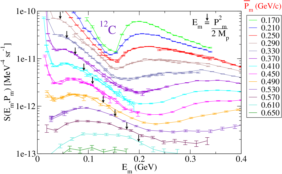
Figure 54: Reduced spectral function for ${}^{12}\textrm{C}$ in the short-range correlated region obtained with $(e,e^{\prime}p)$ reaction [188]. At missing energies above 150 MeV, sizable contributions from the excitation of a $\Delta$ resonance are seen. The arrows indicate indicate the location of the maximum of the spectral function expected according to a simplified picture.

We note that one limiting issue in taking measurements at higher missing energies comes from the necessity of transferring a large amount of energy from the probe to the struck nucleon. The outgoing proton in an experiment that probes this high-energy region can have kinetic energies of several hundreds of MeV, leading to strong rescattering effects, excitation of nucleon resonances, etc. In certain kinematical conditions the associated final state effects can overwhelm the direct process. This has been the case for some previous experiments [271, 272, 273]. The issue of how to minimize the FSI has been addressed in Ref. [186]. There, it is shown that FSI in exclusive $(e,e^{\prime}p)$ cross sections are dominated by two-step processes that become particularly relevant when perpendicular kinematics are employed to probe the regions of small spectral strength. A study of the kinematic conditions shows that for perpendicular kinematics the rescattered nucleons move spectral strength in the $k$-$E$ plane, from the top of the ridge toward regions where the correlated strength is small, therefore submerging the direct signal in a large background noise. In Ref. [186], it was suggested that the contribution of rescattering can be diminished using parallel kinematics. The Jefferson Lab data discussed here was therefore taken in these conditions [187, 188]. First calculations of the rescattering process appear to confirm the expected trend with respect to the kinematics [269, 270]

We also note that other important contributions to the yield of this experiment are expected to come from $(e,e^{\prime}\Delta)$ reactions followed by the decay of the $\Delta$ resonance. The broad peak due to the excitation of the $\Delta$ is clearly visible on the right hand side of Fig. 54. For heavier nuclei or when perpendicular kinematics are used, the above rescattering effects are seen to become more and more relevant and at the same time the strength from the delta region tends to come at low missing energy, filling the gap that separates it from correlated region. Therefore a proper treatment of final state interactions becomes necessary to study the behavior of the strength in the short-range region when the size of the nucleus is increased [270]. First calculations in this direction have been reported in Refs. [269, 270].

The relevance of the experiments discussed in this section lies in the fact that they extend the experimental knowledge of correlations to the regions of the momentum-energy plane that were previously inaccessible. Being able to identify high-momentum components [188] in addition to locating all the sp strength associated with the mean-field orbits [144, 145] completes the search for the missing protons.

6 What a proton does in the nucleus and comparison with other fermion systems

From the results discussed sofar it is clear that a crucial role in obtaining pertinent information about the properties of protons in the nucleus has been played by coincidence experiments involving electron beams. In the following we will therefore summarize on what has been learned in general terms about the properties of these protons. Before embarking on this overview, it is important to note that recent work on single-nucleon knockout with fast radioactive beams [225] proposes to extend this information for valence protons to neutrons and unstable nuclei. Some promising work in this direction has been reported in Refs. [274, 275]. Indeed, there is a long tradition with hadronic probes to study spectroscopic factors in nuclei. Due to the inherent complexity of hadron-induced reactions it has been more difficult to establish absolute spectroscopic factors from corresponding experimental data. Nevertheless, it is possible to generate a consistent analysis of (e,e^′p) and (d,³He) experiments as shown in Ref. [224]. The original discrepancies between these different experiments disappear when a new analyis of the (d,³He) experiments is performed using finite-range DWBA procedures combined with bound-state wave functions obtained from the analysis of (e,e^′p) reactions. The resulting spectroscopic factors then appear to be quite consistent with the spectroscopic factors obtained from the (e,e^′p) reaction [224]. This observation demonstrates that with proper care it is possible to generate valuable information from hadron-induced nucleon knockout experiments. It may therefore be possible to extend the extraction of spectroscopic factors to nuclei far off stability. This exciting new development will allow the study of the properties of nucleons in the nuclear medium in different regions of the periodic table and may provide new challenges for our theoretical understanding.

The present situation concerning the knowledge of the properties of protons in the nucleus may be summarized as follows. The consequences of short-range correlations in nuclear systems on the properties of protons appear to be theoretically well understood and becoming available for experimental scrutiny as discussed in Sec. 5. These results show that the effect of SRC is two-fold. First, it involves the depletion of spectroscopic strength from the mean-field domain as discussed in Sec. 5.9 for the experimental data obtained for ²⁰⁸Pb. These data show that this depletion in heavy nuclei corresponds to about 15% for all the deeply bound proton levels. This result was predicted more than ten years ago based on nuclear-matter calculations briefly reviewed in Sec. 4.2. For lighter nuclei all theoretical work suggests that this amount may be closer to 10% as discussed in Sec. 5.2. Accompanying this information is the realization that valence shells near the Fermi energy will not contain substantial amounts of high-momentum components. This has been experimentally confirmed and clarifies the other role played by SRC in nuclei, i. e. the admixtures of high-momentum components at high missing energy to account for the missing protons removed from the mf location. Recent attempts to quantify the amount of this strength and the corresponding location have been presented in Sec. 5.9. It now appears that about the right amount of high-momentum strength can be identified in the expected region although additional work is needed to complete the analysis. The location of these high-momentum components nevertheless broadly conforms with the mechanism that admixes these correlations with 2h1p states at large missing energies as discussed in Sec. 5.9.

Being able to identify high-momentum components in addition to locating all the sp strength associated with the mean-field orbits [144, 145] completes the identification of the properties of protons in the ground state of the nucleus. The latter understanding is illustrated in Fig. 55.

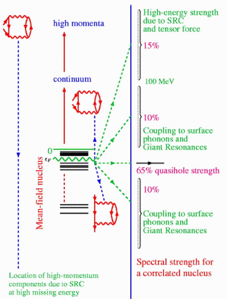
Figure 55: The distribution of single-particle strength in a nucleus like ²⁰⁸Pb. The present summary is a synthesis of experimental and theoretical work discussed in this review. A slight reduction (from 15% to 10%) of the depletion effect due to SRC must be considered for light nuclei like ¹⁶O.

Several generic diagrams are identified in Fig. 55 which have unique physical consequences for the redistribution of the single-particle strength when they are taken into account in the solution of the Dyson equation as discussed in this paper. The middle column of the figure characterizes the mean-field picture that is used as a starting point of the theoretical description. The right column identifies the location of the sp strength of the orbits just below the Fermi energy when correlations are included. One may apply this picture for example to the $3s_{1/2}$ proton orbit in ${}^{208}\textrm{Pb}$. The physical mechanisms responsible for the correlated strength distribution are also identified. The strength of this orbit remaining at the quasihole energy is about 65%. Long-range correlations are responsible for the loss of 20% of the strength due to the coupling to nearby 2p1h and 2h1p states. This loss is symmetrically distributed above and below the Fermi energy and is physically represented by the coupling to low-lying surface modes and higher-lying giant resonances. The resulting occupation number of this orbit therefore corresponds to 75%. More deeply bound nucleons have higher occupation numbers corresponding to 85%. As discussed in Sec. 5.9 this is true for all these deep-lying orbits and is consistent with a global depletion due to SRC of 15%. The corresponding location of this strength is identified at very high energy in the particle domain and is due to the short-range and tensor correlations induced by a realistic nucleon-nucleon interaction as discussed in Sec. 4. In the left column of Fig. 55 the generic diagram that is responsible for the admixture of high-momentum components in the ground state is depicted. The energy domain of these high-momentum nucleons is at large missing energies as discussed above.

This rather complete picture of the properties of a strongly interacting proton in the nucleus signals a unique position for the field of nuclear physics. Indeed, unlike other fields with strong correlations effects, like particle or condensed matter physics, it is now possible in nuclear physics to state that the properties of the constituent protons inside the nucleus are identified experimentally and understood in global terms theoretically. For atoms and molecules it is also possible to extract this kind of information by employing the corresponding (e,2e) reaction [276, 277]. This reaction generates the best possible information on the properties of individual electrons in these systems. Indeed, it was shown in 1981 that one can “measure” the square of the $1s$ wave function of the Hydrogen atom in momentum space [278]. Similar results for electron wave functions in the medium have been obtained for a wide range of atoms and molecules [276]. Similar wave function results for nuclei are given in Fig. 10 of Sec. 3. This technique may also become successful in identiying the properties of electrons in solids [279]. In nuclear physics the improved analysis of two-nucleon knockout reactions is expected to provide detailed information about the short-range interaction of nucleons in the nuclear medium. With the additional improvement of the analysis of experiments that probe high-momentum nucleons in the nucleus, one may therefore look forward to an even deeper understanding of nucleon properties and their interactions in the future.

7 Summary and Outlook

Several recent developments have been reported that are of general importance to the understanding of nuclei. We single out here the improved understanding of the nuclear-matter saturation problem and in particular the essentially complete understanding of the properties of protons in nuclei. These achievements have been accomplished by applying the method of self-consistent Green’s function. This method has been presented in this overview together with a summary of the calculations that have been performed in nuclear physics. One of the motivations to employ this method is that the quantities that form the ingredients of the calculations have a very clear relationship with experimental data. This is true for the one-body propagator which contains information about one-nucleon removal (and addition) quantities but also for other propagators discussed in this work. These include the polarization propagator which yields information about excited states and corresponding transition probabilities but also the pp(hh) propagator which for the hh part can be related to two-nucleon knockout data. The appearance of all these quantities as ingredients of self-consistent calculations provides us with a multitude of opportunities to compare theory with experimental data. One of the strengths of the method is therefore its ability to identify relevant physical correlations that need to be included in the calculation based on this comparison with experiment. As an example, the fragmentation of the removal strength observed in nuclei immediately identifies the need for a dynamic content of the self-energy of a nucleon below the Fermi energy. The comparison of the theoretical sp strength distribution obtained with the second-order self-energy with experimental data then immediately points to the need for a better description of the intermediate states in the self-energy. This in turn leads to the consideration of the coupling to collective motion at low energy. The process is illustrated by the development of the Faddeev technique to the many-body problem discussed in Sec. 5 which allows the inclusion of these collective features of both ph as well as pp(hh) character. In turn, these microscopic phonons yield information that can be directly compared with the excitation spectra in the corresponding nuclei with $A$ and $A\pm 2$ nucleons. This comparison suggests further improvements of these phonons which in turn can be taken into account in describing the sp properties and so on.

Another important advantage of the SCGF method is associated with its ability to handle the relevant physical correlations. As has been discussed throughout this review the treatment of SRC can be handled by the summation of ladder diagrams whereas for LRC it appears that the Faddeev technique is necessary in finite nuclei. The treatment of SRC is most advanced for nuclear matter where the method is applied by several groups but for finite nuclei improvements should be studied in the future. The discussion of the results for the saturation properties of nuclear matter with the inclusion of SRC as given in Sec. 4.7 suggests that it may be important to actually establish the validity of one of the underlying assumptions of the nuclear-matter problem. This assumption is that the best equation of state for a given Hamiltonian will automatically yield information relevant for finite nuclei. This assumption has been questioned in this review since it is unclear that long-range pionic modes which contribute significantly to nuclear-matter binding actually play a significant role in finite nuclei. We therefore urgently suggest investigations which clearly identify whether pion-exchange in ²⁰⁸Pb is really similar to the corresponding process in nuclear matter. If the answer is negative, nuclear physicists may have worried too much in the past about their inability to describe the empirical saturation properties of nuclear matter.

It has been argued in this review that it has been possible to track the properties of all the protons in closed-shell nuclei. We emphasize that this achievement reflects the combined effort of experiment and theory. The arrival of new facilities which aim to probe the properties of nuclei far off stability will also provide us with new challenges to theory. The inclusion of the continuum in SCGF calculations is a technical challenge but the method appears sufficiently flexible to include this difficulty. Knowledge of the sp properties of these exotic nuclei will widen the scope of our understanding of the properties of nucleons in nuclei. Additional work is also necessary to improve the description of the spectrum and sp strength in ¹⁶O. It appears likely that the Faddeev method can be applied to study the low-energy properties associated with particle addition (elastic scattering) which also has relevance to astrophysical problems. The flexibility of this method is not restricted to nuclear physics and may also be applied to other many-body systems like the electron gas.

References

- [1]
- [2] H. Müther and A. Polls, Prog. Part. Nucl. Phys. 45, 243 (2000).
- [3] A. A. Abrikosov, L. P. Gorkov and I. E. Dzyaloshinski, Methods of Quantum Field Theory in Statistical Physics (Dover, New York, 1975).
- [4] P. Nozières, Theory of Interacting Fermion Systems (Addison-Wesley, Reading MA, 1997)
- [5] P. C. Martin and J. Schwinger, Phys. Rev. 115, 1342 (1959).
- [6] A. B. Migdal, Theory of Finite Fermi Systems (Wiley, New York, 1967)
- [7] A. L. Fetter and J. D. Walecka, Quantum Theory of Many-Particle Physics (McGraw-Hill, New York, 1971).
- [8] D. Van Neck, K. Peirs, and M. Waroquier, J. Chem. Phys. 115, 15 (2001).
- [9] B. Holm and U. von Barth, Phys. Rev. B 57, 2108 (1998).
- [10] D. M. Ceperly and B. J. Alder, Phys. Rev. Lett. 45, 566 (1980).
- [11] S. Frullani and J. Mougey, Adv. Nucl. Phys. 14, 1 (1984) .
- [12] P. K. A. de Witt Huberts, J. Phys. G: Nucl. Part. Phys. 16, 507 (1990).
- [13] A. E. L. Dieperink and P. K. A. de Witt Huberts, Ann. Rev. Nucl. Part. Sci. 40, 239 (1990).
- [14] I. Sick and P. de Witt Huberts, Comm. Nucl. Part. Phys. 20, 177 (1991).
- [15] L. Lapikás, Nucl. Phys. A553, 297c (1993).
- [16] V. R. Pandharipande, I. Sick, and P. K. A de Witt Huberts, Rev. Mod. Phys. 69, 981 (1997).
- [17] S. Boffi, C. Giusti, F. D. Pacati, and M. Radici, Electromagnetic Response of Atomic nuclei, Oxford Studies in Nuclear Physics (Clarendon, Oxford, 1996).
- [18] V. M. Galitski, Sov. Phys.-JETP 7, 104 (1958).
- [19] L. C. Gomes, J. D. Walecka, and V. F. Weisskopf, Ann. Phys. 3, 241 (1958).
- [20] B. D. Day, Rev. Mod. Phys. 39, 719 (1967).
- [21] S. C. Pieper and R. B. Wiringa, Ann. Rev. Nucl. Part. Sci. 51, 53 (2001)
- [22] P. Navratil and W. E. Ormand, Phys. Rev. C 68, 034305 (2003).
- [23] H. Lehmann, Nuovo Cimento 11, 342 (1952).
- [24] A. E. L. Dieperink and T. de Forest, Jr. Phys Rev. C 10, 543 (1974).
- [25] J. Escher and B. K. Jennings, Phys. Rev. C 66, 034313 (2002).
- [26] V. M. Galitski and A. B. Migdal, Sov. Phys.-JETP 7, 96 (1958).
- [27] D. S. Koltun, Phys. Rev. C 9, 484 (1974).
- [28] J. W. Negele and H. Orland, Quantum Many-Particle Systems (Perseus Books, Massachusetts, 1988).
- [29] G. Baym and L. P. Kadanoff, Phys. Rev. 124, 287 (1961).
- [30] L. P. Kadanoff and G. Baym, Quantum Statistical Mechanics (W.A. Benjamin, Menlo Park, 1962).
- [31] G. Baym, Phys. Rev. 127, 1391 (1962).
- [32] C. Barbieri and W. H. Dickhoff, Phys. Rev. C 63, 034313 (2001).
- [33] P. Ring and P. Schuck, The Nuclear Many-body Problem (Springer, New York, 1980).
- [34] D. Pines and D. Bohm, Phys. Rev. 85, 338 (1952).
- [35] D. Bohm and D. Pines, Phys. Rev. 92, 609 (1953).
- [36] D. Pines, Phys. Rev. 92, 626 (1953).
- [37] K. A. Brueckner, C. A. Levinson, and H. M. Mahmoud, Phys Rev. 95, 217 (1954).
- [38] J. Goldstone, Proc. Roy. Soc. (London) A239, 267 (1957).
- [39] C. Mahaux and R. Sartor, Adv. Nucl. Phys. 20, 1 (1991).
- [40] E. N. M. Quint, Ph.D. thesis, University of Amsterdam (1988).
- [41] G.J. Wagner, AIP Conf. Proc. 142, 220 (1986).
- [42] P. Grabmayr et al., Phys. Lett. B164, 15 (1985).
- [43] P. Grabmayr, Prog. Part. Nucl. Phys. 29, 251 (1992).
- [44] K. Gottfried, Nucl. Phys. 5, 557 (1958).
- [45] C. Ciofi degli Atti, in Two Nucleon Emission Reactions, O. Benhar and A. Fabrocini, eds. (ETS Editrice, Pisa, 1990), p.1.
- [46] O. Benhar, A. Fabrocini, and S. Fantoni, in Two Nucleon Emission Reactions, O. Benhar and A. Fabrocini, eds. (ETS Editrice, Pisa, 1990), p.49.
- [47] S. Boffi, in Two Nucleon Emission Reactions, O. Benhar and A. Fabrocini, eds. (ETS Editrice, Pisa, 1990), p.87.
- [48] C. Giusti and F. D. Pacati, Nucl. Phys. A535, 573 (1991).
- [49] C. Giusti, F. D. Pacati, and M. Radici, Nucl. Phys. A546, 607 (1992).
- [50] C. Giusti and F. D. Pacati, Nucl. Phys. A571, 694 (1994).
- [51] C. Giusti and F. D. Pacati, Nucl. Phys. A585, 618 (1995).
- [52] L. J. H. M. Kester et al., Phys. Rev. Lett. 74, 1712 (1995).
- [53] J. Ryckebusch, Nucl. Phys. A568, 828 (1994).
- [54] L. J. H. M. Kester, Ph.D. thesis, NIKHEF, Amsterdam (1993).
- [55] W. H. Dickhoff and H. Müther, Rep. Prog. Phys. 55, 1947 (1992).
- [56] A. Ramos, Beyond a mean-field description of nuclear systems within self-consistent Green functions theory, Ph.D. thesis, University of Barcelona (1988).
- [57] A. Ramos, A. Polls, and W. H. Dickhoff, Nucl. Phys. A503, 1 (1989).
- [58] O. Benhar, A. Fabrocini, and S. Fantoni, Nucl. Phys. A505, 267 (1989).
- [59] O. Benhar, A. Fabrocini, and S. Fantoni, Nucl. Phys. 550, 201 (1992).
- [60] R. V. Reid, Ann. Phys. 50, 411 (1968).
- [61] B. E. Vonderfecht, W. H. Dickhoff, A. Polls, and A. Ramos, Phys. Rev. C 44, R1265 (1991).
- [62] B. E. Vonderfecht, W. H. Dickhoff, A. Polls, and A. Ramos, Nucl. Phys. A555, 1 (1993).
- [63] B. E. Vonderfecht, Short-range correlations and superfluidity in the Green’s function theory for nuclear matter, Ph.D. thesis, Washington University in St. Louis (1991).
- [64] B. E. Vonderfecht, C. C. Gearhart, W. H. Dickhoff, A. Polls, and A. Ramos, Phys. Lett. B253, 1 (1991).
- [65] C. C. Gearhart, Self-consistently dressed nucleons and nuclear wave functions, Ph.D. thesis, Washington University in St. Louis (1994).
- [66] C. C. Gearhart, W. H. Dickhoff, A. Polls, and A. Ramos, Int. J. Mod. Phys. E 5, 261 (1996).
- [67] W. H. Dickhoff, C. C. Gearhart, E. P. Roth, A. Polls, and A. Ramos, Phys. Rev. C 60, 064319 (1999).
- [68] P. Bożek, Phys. Lett. B551, 93 (2003).
- [69] F. de Jong and H. Lenske, Phys. Rev. C 56, 2619 (1997).
- [70] P. Bożek, Nucl. Phys. A657, 187 (1999).
- [71] J. Lehr, M. Effenberger, H. Lenske, S. Leupold, and U. Mosel, Phys. Lett. B483, 324 (2000).
- [72] Y. Dewulf, Self-consistent Green’s function approach to short-range correlations in nuclear matter, Ph.D. thesis, University of Gent (2000).
- [73] E. P. Roth (Stoddard), Self-consistent Green’s functions in nuclear matter, Ph.D. thesis, Washington University in St. Louis (2000).
- [74] Y. Dewulf, D. Van Neck, and M. Waroquier, Phys. Lett. B510,89 (2001).
- [75] T. Frick, K. Gad, H. Müther, and P. Czerski, Phys. Rev. C 65, 034321 (2002).
- [76] Y. Dewulf, D. Van Neck, and M. Waroquier, Phys. Rev. C 65, 054316 (2002).
- [77] P. Bożek, Phys. Rev. C 65, 054306 (2002).
- [78] P. Bożek, Eur. Phys. J. A15, 325 (2002).
- [79] W. H. Dickhoff and E. P. Roth, Acta Phys. Pol. B 33, 65 (2002).
- [80] V. G. J. Stoks, R. A. M. Klomp, C. P. F. Terheggen, and J. J. de Swart, Phys. Rev. C 49, 2950 (1994).
- [81] J. Haidenbauer and W. Plessas, Phys. Rev. C 30, 1822 (1984).
- [82] J. Haidenbauer and W. Plessas, Phys. Rev. C 32, 1424 (1985).
- [83] Y. Dewulf, W. H. Dickhoff, E. R. Stoddard, D. Van Neck, and M. Waroquier, Phys. Rev. Lett. 90, 152501 (2003).
- [84] N. J. Robertson, Effects of short-range correlations on decay in nuclear matter, Ph.D. thesis, Washington University in St. Louis (2003).
- [85] W.H. Dickhoff, Phys. Rev. C 58, 2807 (1998).
- [86] A. Ramos, W. H. Dickhoff, and A. Polls, Phys. Lett. B219, 15 (1989).
- [87] E. Schiller, H. Müther, and P. Czerski, Phys. Rev. C 59, 2934 (1999); ibid. 60, 059901 (1999) .
- [88] K. Suzuki, R. Okamoto, M. Kohno, and S. Nagata, Nucl. Phys. A665, 92 (2000).
- [89] L.D. Landau, Soviet Phys.-JETP 3, 920 (1957); 5, 101 (1957); 8, 70 (1958).
- [90] G. E. Brown, Comm. Nucl. Part. Phys. 3, 136 (1969).
- [91] S. Fantoni and V. R. Pandharipande, Nucl. Phys. A427, 473 (1984).
- [92] P. Grangé, J. Cugnon, and A. Lejeune, Nucl. Phys. A473, 365 (1987).
- [93] M. Baldo et al., Phys. Rev. C 41, 1748 (1990).
- [94] A. Gal, Adv. Nucl. Sci. 8, 1 (1977).
- [95] B. Povh, Ann. Rev. Nucl. Sci. 28, 1 (1978)
- [96] C. B. Dover and A. Gal, Prog. Part. Nucl. Phys. 12, 171 (1983)
- [97] T. Motoba, M. Bandō, R. Wünsch, and J. Žofka, Phys. Rev. C 38, 1322 (1989).
- [98] A. A. Usmani, S. C. Pieper, and Q. N. Usmani, Phys. Rev. C 51, 2347 (1995).
- [99] D. Halderson, Phys. Rev. C 61, 034001 (2000).
- [100] J. Rożynek and J. Da̧browski, Phys. Rev. C 20, 1612 (1979).
- [101] Y. Yamamoto, H. Bandō, Prog. Theor. Phys. 73, 189 (1983).
- [102] Y. Yamamoto, and H. Bandō, Prog. Theor. Phys. 83, 254 (1990).
- [103] A. Reuber, K. Holinde, and J. Speth, Nucl. Phys. A570, 543 (1994).
- [104] H.-J. Schulze, A. Lejeune, J.Cugnon, M. Baldo,and U. Lombardo, Phys. Lett. B355, 21 (1995).
- [105] H.-J. Schulze, M.Baldo, U. Lombardo, J. Cugnon, and A. Lejeune, Phys. Rev. C 57, 704 (1998).
- [106] J. Da̧browski and J. Rożynek, Prog. Theor. Phys. 105, 923 (2001).
- [107] M. M. Nagels, T. A. Rijken, and J. J. de Swart, Phys. Rev. D 12, 744 (1975).
- [108] M. M. Nagels, T. A. Rijken, and J. J. de Swart, Phys. Rev. D 15, 2547 (1977).
- [109] M. M. Nagels, T. A. Rijken, and J. J. de Swart, Phys. Rev. D 20, 1633 (1979).
- [110] P. M. M. Maessen, T. A. Rijken, and J. J. de Swart, Phys. Rev. C 40, 2226 (1989).
- [111] B. Holzenkamp, K. Holinde, and J. Speth, Nucl. Phys. A500, 485 (1989).
- [112] T. A. Rijken, V. G. J. Stoks, and Y. Yamamoto, Phys. Rev. C 59, 21 (1999).
- [113] N. J. Robertson and W. H. Dickhoff, Phys. Rev. C, to be published.
- [114] W.H. Dickhoff, Phys. Rep. 242, 119 (1994).
- [115] R.F. Bishop, H.B. Ghassib, and M.R. Strayer, Phys. Rev. A 13, 1570 (1974).
- [116] K. Gottfried Quantum Mechanics (Addison-Wesley, Redwood City CA, 1989).
- [117] F.A. Brieva and J.R. Rook, Nucl. Phys. A291, 299 (1977).
- [118] G.F. Bertsch and S. Das Gupta, Phys. Reports 160, 189 (1988).
- [119] W. Bauer, C.-K. Gelbke, and S. Pratt, Annu. Rev. Nucl. Part. Sci. 42, 77 (1992).
- [120] T. Alm, G. Röpke, W. Bauer, F. Daffin, and M. Schmidt, Nucl. Phys. A587, 815 (1995).
- [121] B. ter Haar and R. Malfliet, Phys. Rev. C 36, 1611 (1987).
- [122] A. Bohnet, N. Ohtsuka, J. Aichelin, R. Linden, and A. Faessler, Nucl. Phys. A494, 349 (1989).
- [123] A. Faessler, Nucl. Phys. A495, 103c (1989).
- [124] M. Schmidt, G. Röpke, and H. Schulz, Ann. Phys. (N.Y.) 202, 57 (1990).
- [125] G.Q. Li and R. Machleidt, Phys. Rev. C 48, 1702 (1993).
- [126] G.Q. Li and R. Machleidt, Phys. Rev. C 49, 566 (1994).
- [127] T. Alm, G. Röpke, and M. Schmidt, Phys. Rev. C 50, 31 (1994).
- [128] G. Giansiracusa, U. Lombardo, and N. Sandalescu, Phys. Rev. C 53, R1478 (1996).
- [129] H.-J. Schulze, A. Schnell, G. Röpke, and U. Lombardo, Phys. Rev. C 55, 3006 (1997).
- [130] A. Schnell, G. Röpke, U. Lombardo, and H.-J. Schulze, Phys. Rev. C 57, 806 (1998).
- [131] T. Alm, G. Röpke, and M. Schmidt, Z. Phys. A 337, 355 (1990).
- [132] M. Baldo, I. Bombaci, and U. Lombardo, Phys. Lett. B283, 8 (1992).
- [133] O. Benhar et al., Nucl. Phys. A703, 70 (2002).
- [134] B. D. Day, Phys. Rev. C 24, 1203 (1981).
- [135] H. Q. Song, M. Baldo, G. Giansiracusa, and U. Lombardo, Phys. Rev. Lett. 81, 1584 (1998).
- [136] R. B. Wiringa, R. A. Smith, and T. L. Ainsworth, Phys. Rev. C 29, 1207 (1984).
- [137] B. D. Day and R. B. Wiringa, Phys. Rev. C32, 1057 (1985).
- [138] J. Carlson, V. R. Pandharipande, and R. B. Wiringa, Nucl. Phys. 401, 59 (1983).
- [139] R. B. Wiringa, V. Fiks, and A. Fabrocini, Phys Rev. C 38, 1010 (1988).
- [140] M. R. Anastasio, L.S. Celenza, W. S. Pong, and C. M. Shakin, Phys. Rep. 100, 327 (1983).
- [141] B. ter Haar and R. Malfliet, Phys. Rev. Lett. 56, 1237 (1986).
- [142] R. Brockmann and R. Machleidt, Phys. Rev. C 42, 1965 (1990).
- [143] A. Amorim and J. A. Tjon, Phys. Rev. Lett. 68, 772 (1992).
- [144] L. Lapikás et al., to be submitted to Phys. Rev. Lett. (2004).
- [145] M. F. van Batenburg, Ph.D. thesis, University of Utrecht (2001).
- [146] G. A. Rijsdijk, K. Allaart, and W. H. Dickhoff, Nucl. Phys. A550, 159 (1992).
- [147] V.R. Pandharipande, C.N. Papanicolas, and J. Wambach, Phys. Rev. Lett. 53, 1133 (1984)
- [148] O. Benhar et al., Phys. Rev. C 41, R24 (1990).
- [149] D. Rohe, Proc. 5th Workshop on “e-m induced Two-Hadron Emission”, 2001, Lund, Sweden (CD ISBN:91-631-1612-X) 67.
- [150] C. Ciofi degli Atti, S. Liuti, and S. Simula, Phys. Rev. C 41, R2474 (1990).
- [151] H. Müther, A. Polls, and W. H. Dickhoff, Phys. Rev. C 51, 3040 (1995).
- [152] I. Bobeldijk et al., Phys. Rev. Lett. 73, 2684 (1994).
- [153] B. Frois et al., Phys. Rev. lett 38, 152 (1977).
- [154] T. R. Mongan, Phys. Rev. 178, 1597 (1969).
- [155] J. P. Blaizot, J. F. Berger, J. Dechargé and M. Girod, Nucl.Phys. A591, 435 (1995)
- [156] W. H. Dickhoff, A. Faessler, and H. Müther, Nucl. Phys. A389, 492 (1982).
- [157] A. D. Jackson, A. Landé, and R. A. Smith, Phys. Rep. 86, 55 (1982).
- [158] A. B. Migdal, Rev. Mod. Phys. 50, 107 (1978).
- [159] W. H. Dickhoff, A. Faessler, J. Meyer-ter-Vehn, and H. Müther, Phys. Rev. C 23, 1154 (1981).
- [160] W. H. Dickhoff, Prog. Part. Nucl. Phys. 12, 529 (1983).
- [161] P. Czerski, H. Müther, and W. H. Dickhoff, J. Phys. G: Nucl. Part. Phys. 20, 425 (1994).
- [162] P. Czerski, W. H. Dickhoff, A. Faessler, and H. Müther, Phys. Rev. C 33, 1753 (1986).
- [163] W. Alberico, et al, Phys. Rev. C 34, 977 (1986).
- [164] T. A. Carey et al., Phys. Rev. Lett. 53, 144 (1984).
- [165] T. N. Taddeucci et al., Phys. Rev. Lett. 73, 3516 (1994).
- [166] T. Wakasa et al., Phys. Rev. C 59, 3177 (1999).
- [167] S. C. Pieper et al., Phys. Rev. C 64, 014001 (2001).
- [168] R. B. Wiringa et al., Phys. Rev. C 62, 014001 (2000).
- [169] J.G. Zabolitzky and W. Ey, Phys. Lett. B76, 527 (1978).
- [170] J.W. Van Orden, W. Truex, and M.K. Banerjee, Phys. Rev. C 21, 2628 (1980).
- [171] O. Benhar, C. Ciofi degli Atti, S. Liuti, and G. Salmè, Phys. Lett. B177, 135 (1986).
- [172] X. Ji and J. Engel, Phys. Rev. C 40, R497 (1989).
- [173] S. Stringari, M. Traini, and O. Bohigas, Nucl. Phys. A516, 33 (1990).
- [174] S.C. Pieper, R.B. Wiringa, and V.R. Pandharipande, Phys. Rev. C 46, 1741 (1992).
- [175] H. Morita and T. Suzuki Prog. Theo. Phys. 86, 671 (1991).
- [176] S. Tadokoro, T. Katyama, Y. Akaishi, and H. Tanaka, Prog. Theor. Phys. 78, 732 (1987).
- [177] C. Ciofi degli Atti, E. Pace, and G. Salmè, Phys. Lett. B141, 14 (1984).
- [178] O. Benhar and V.R. Pandharipande, Phys. Rev. C 47, 2218 (1993).
- [179] I. Sick, A. Fantoni, A. Fabrocini, and O. Benhar, Phys. Lett. B323, 267 (1994).
- [180] O. Benhar, A. Fabrocini, S. Fantoni, and I. Sick, Nucl. Phys. A579, 493 (1994).
- [181] D. Van Neck, A.E.L. Dieperink, and E. Moya de Guerra, Phys. Rev. C 51, 1800 (1995).
- [182] M. Radici, S. Boffi, S C. Pieper, and V. R. Pandharipande, Phys. Rev. C 50, 3010 (1994).
- [183] A. Fabrocini and G. Co’, Phys. Rev. C 63, 044319 (2001).
- [184] H. Müther and W. H. Dickhoff, Phys. Rev. C 49, R17 (1994);
- [185] A. Polls, and H. Müther, W. H. Dickhoff, Nucl. Phys. A594, 117 (1995).
- [186] I. Sick, et al., Jlab-Proposal E97-006, (1997).
- [187] D. Rohe, Eur. Phys. J. A17, 439 (2003), (Conference proceeding on Electron-Nucleus Scattering VII in Elba 2002)
- [188] D. Rohe, Proc. 6th Workshop on “e-m induced Two-Hadron Emission”, 2003, Pavia, Italy. To be published.
- [189] M.G.E. Brand, G.A. Rijsdijk, F.A. Muller, K. Allaart, and W.H. Dickhoff, Nucl. Phys. A531, 253 (1991).
- [190] D. Van Neck, M. Waroquier, and J. Ryckebusch Nucl. Phys. A530, 347 (1991).
- [191] D. Van Neck, M. Waroquier, V. Van der Sluys and K. Heyde, Nucl. Phys. A563, 1 (1993).
- [192] H. Müther and L.D. Skouras, Phys. Lett. B306, 201 (1993).
- [193] J. Yuan, Ph.D. thesis, Washington University, St. Louis, 1994.
- [194] H. Müther and L.D. Skouras, Nucl. Phys. A581, 247 (1995).
- [195] K. Amir-Azimi-Nili, H. Müther, L. D. Skouras, and A. Polls, Nucl. Phys. A604, 245 (1996).
- [196] W. J. W. Geurts, K. Allaart, W. H. Dickhoff, and H. Müther, Phys. Rev. C 53, 2207 (1996).
- [197] C. Barbieri and W. H. Dickhoff, Phys. Rev. C 65, 064313 (2002)
- [198] D. Van Neck, M.Waroquier, A. E. L. Dieperink, S C. Pieper, and V. R. Pandharipande, Phys. Rev. C 57, 2308 (1998).
- [199] M. Leuschner et al., Phys. Rev. C 49, 955 (1994).
- [200] C. Barbieri and W. H. Dickhoff, Phys. Rev. C 68, 014311 (2003)
- [201] W. H. Dickhoff, Nucl. Phys. A399 (1983) 287.
- [202] G. Kramer, Ph.D. Thesis, University of Amsterdam (1990).
- [203] M. Borromeo, D. Bonatsos, H. Müther, and A. Polls, Nucl. Phys. A539, 189 (1992).
- [204] D. Bonatsos and H. Müther, Nucl. Phys. A496, 23 (1989).
- [205] C. W. Wong and D. M. Clement, Nucl. Phys. A183, 210 (1972).
- [206] C. Mahaux, P. F. Bortignon, R. A. Broglia and C. H. Dasso, Phys. Rep. 120, 1 (1985).
- [207] R. Machleidt, Adv. Nucl. Phys. 19, 191 (1989).
- [208] Z.Y. Ma and J. Wambach, Phys. Lett. B256, 1 (1991).
- [209] J. Al-Khalili, C. Barbieri, J. Escher, B. K. Jennings and J. M. Sparenberg, Phys. Rev. C 68, 024314 (2003)
- [210] A. Polls, M. Radici, S. Boffi, W. H. Dickhoff and H. Müther, Phys. Rev. C 55, 810 (1997).
- [211] G.Có,, A. Fabrocini, and S. Fantoni, Nucl. Phys. A568, 73 (1994).
- [212] C. Ciofi degli Atti, S. Simula, L.L. Frankfurt, and M.I. Strikman, Phys. Rev. C44, R7 (1991).
- [213] W.H. Dickhoff, P.P. Domitrovich, A. Polls, and A. Ramos, in Condensed Matter Theories, edited by V.C. Aguilera-Navarro (Plenum, New York, 1990), Vol. 5, p.275; P.P. Domitrovich, thesis, Washington University, 1991.
- [214] J. Mougey, Nucl. Phys. A335, 35 (1980).
- [215] H. Müther, G. Knehr, and A. Polls, Phys. Rev. C 52, 2955 (1995).
- [216] E. K. Warburton, B. A. Brown, and D. J. Millener, Phys. Lett. B293, 7 (1992).
- [217] M. Homma, T. Mizusaki, and T. Otsuka, Phys. Rev. Lett. 75, 1284 (1995).
- [218] L. D. Faddeev, Sov. Phys. JETP 12, 1014 (1961).
- [219] C. J. Joachain Quantum Collision Theory, (North-Holland, Amsterdam, 1975).
- [220] W. Glöckle, The Quantum Mechanical Few-Body Problem (Springer, Berlin, 1983).
- [221] C. Barbieri, Self-consistent Green’s functions study of low-energy correlations in , Ph.D. thesis, Washington University in St. Louis (2002).
- [222] W. J. W. Geurts, K. Allaart, and W. H. Dickhoff, Phys. Rev. C 50, 514 (1994).
- [223] H. Müther and P. Sauer, in Computational Nuclear Physics ed. by K.-H. Langanke, et al. (Springer Berlin, 1993).
- [224] G. J. Kramers, H. P. Blok, and L. Lapikás, Nucl. Phys. A679, 267 (2001).
- [225] P. G. Hansen and J. A. Tostevin, Ann. Rev. Nucl. Part. Sci. 53, 219 (2003).
- [226] M. G. E. Brand, K. Allaart, and W. H. Dickhoff, Phys. Lett. B214, 483 (1988);
- [227] M. G. E. Brand, K. Allaart, and W. H. Dickhoff, Nucl. Phys. A509, 1 (1990).
- [228] W. H. Dickhoff, in Condensed Matter Theories. Vol. 3, ed. J. S. Arponen, R. F. Bishop and M. Manninen (Plenum, New York 1988) p. 261.
- [229] F. Ajzenberg-Selove, Nucl. Phys. A375, 1 (1982).
- [230] G. E. Brown, and A. M. Green, Nucl. Phys. 75, 401 (1966);
- [231] W. C. Haxton, and C. J. Johnson, Phys. Rev. Lett. 65, 1325 (1990);
- [232] T. N. Buti et al., Phys. Rev. C 33, 755 (1986).
- [233] H. Feshbach and F. Iachello, Phys. Lett. B45, 7 (1973);
- [234] H. Feshbach and F. Iachello, Ann. Phys. 84, 211 (1974).
- [235] M. S. Zisman, E. A. McClatchie, and B. G. Harvey, Phys. Rev. C 2, 1271 (1970);
- [236] J. Lowe and A. R. Barnett, Nucl. Phys. A187, 323 (1972).
- [237] C. J. G. Onderwater et al., Phys. Rev. Lett. 78 4893 (1997).
- [238] C. J. G. Onderwater et al., Phys. Rev. Lett. 81 2213 (1998).
- [239] D. L. Groep et al., Phys. Rev. Lett. 83 5443 (1999).
- [240] K. I. Blomqvist et al., Phys. Lett. B421 71 (1998).
- [241] G. Rosner, Conference on Perspectives in Hadronic Physics, eds. S. Boffi, C. Ciofi degli Atti, and M. M. Giannini (World Scientific, Singapore, 1998) page 185.
- [242] C. Giusti, F. D. Pacati, K Allaart, W. J. W. Geurts, K. Allaart, W. H. Dickhoff, and H. Müther, Phys. Rev. C 57, 1691 (1998).
- [243] C. Giusti, H. Müther, F. D. Pacati, and M. Stauf Phys. Rev. C 60, 054608 (1999).
- [244] J. Ryckebusch, V. Van der Sluys, K. Heyde, H. Holvoet, W. Van Nespen, and M. Waroquier, Nucl. Phys. A624, 581 (1997);
- [245] Starink et al., Phys. Lett. B474 33 (2000).
- [246] W. J. W. Geurts, K. Allaart, W. H. Dickhoff, and H. Müther, Phys. Rev. C 54, 1144 (1996).
- [247] K. A. Brueckner et al., Phys. Rev. 110, 431 (1958).
- [248] K. A. Brueckner et al., Phys. Rev. 121, 255 (1961).
- [249] O. Benhar et al., Phys. Rev. C 67, 014326 (2003).
- [250] D. Knodler and H. Müther, Phys. Rev. C 63, 044602 (2001).
- [251] M. Schwamb, S. Boffi, C. Giusti, and F. D. Pacati, Eur. Phys. J. A 17, 7 (2003).
- [252] S. Boffi, C. Giusti, and F.D. Pacati, Phys. Rep. 226, 1 (1993).
- [253] J.J. Kelly, Adv. Nucl. Phys. 23, 75 (1996).
- [254] J.M. Udías, P. Sarriguen, E.M. de Guerra, E. Garrido, and J.A. Caballero, Phys. Rev. C 51, 3246 (1995).
- [255] L. Lapikás, G. van der Steenhoven, L. Frankfurt, M. Strikman, and M. Zhalov, Phys. Rev. C 61, 064325 (2000).
- [256] L. Frankfurt, M. Strikman, and M. Zhalov, Phys. Lett. B503, 73 (2001).
- [257] T. de Forest, Nucl. Phys. A392, 232 (1983).
- [258] J.M. Udías, J.A. Caballero, E. Moya de Guerra, J.R. Vignote, and A. Escuderos, Phys. Rev. C 64, 024614 (2001).
- [259] M. Radici, W. H. Dickhoff, and E. Roth Stoddard, Phys. Rev. C 66, 014613 (2002).
- [260] J. Gao et al., the Jefferson Lab Hall A Collaboration, Phys. Rev. Lett. 84, 3265 (2000).
- [261] S. Jeschonnek, Phys. Rev. C 63, 034609 (2001).
- [262] J.J. Kelly, Phys. Rev. C 60, 044609 (1999).
- [263] A. Bianconi and M. Radici, Phys. Rev. C 54, 3117 (1996).
- [264] A. Bianconi and M. Radici, Phys. Rev. C 56, 1002 (1997).
- [265] M. Zhalov, private communication (2001).
- [266] A. Meucci, C. Giusti, and F.D. Pacati, Phys. Rev. C 64, 014604 (2001).
- [267] M. Radici, A. Meucci, and W. H. Dickhoff, Eur. Phys. J. A 17, 65 (2003).
- [268] N.C.R. Makins et al., the NE18 Collaboration, Phys. Rev. Lett. 72, 1986 (1994).
- [269] C. Barbieri, L. Lapikás, and D. Rohe, Proc. 2nd International Conference on Nuclear and Particle Physics with CEBAF at JLab, 2003, Dubrovnik [nucl-th/0309024]
- [270] C. Barbieri and L. Lapikás, Proc. 6th Workshop on “e-m induced Two-Hadron Emission”, 2003, Pavia, Italy. To be published on CD. [nucl-th/0401010]
- [271] H. Baghaei, et al., Phys. Rev. C 39, 177 (1989);
- [272] R. W. Lourie, et al., Phys. Rev. Lett. 56, 1234 (1986).
- [273] L. B. Weinstein, et al., Phys. Rev. Lett. 64, 1646 (1990).
- [274] B. .A. Brown, P. G. Hansen, B. M. Sherrill, and J. A. Tostevin, Phys. Rev. C 65, 061601 (2002).
- [275] J. Enders et al., Phys. Rev. C 67, 064301 (2003).
- [276] I. E. McCarthy and E. Weigold, Rep. Prog. Phys. 54, 789 (1991).
- [277] M. A. Coplan, J. H. Moore, and J. P. Doering, Rev. Mod. Phys. 66, 985 (1994).
- [278] B. Lohmann and E. Weigold, Phys. Lett. A86, 139 (1981).
- [279] M. Vos and I. E. McCarthy, Rev. Mod. Phys. 67, 713 (1995)