Faddeev calculations of break-up reactions with realistic experimental constraints

Abstract

We present a method to integrate predictions from a theoretical model of a reaction with three bodies in the final state over the region of phase space covered by a given experiment. The method takes into account the true experimental acceptance, as well as variations of detector efficiency, and eliminates the need for a Monte-Carlo simulation of the detector setup. The method is applicable to kinematically complete experiments. Examples for the use of this method include several polarization observables in $dp$ break-up at 270 MeV. The calculations are carried out in the Faddeev framework with the CD Bonn nucleon-nucleon interaction, with or without the inclusion of an additional three-nucleon force.

I INTRODUCTION

For nuclear reactions with two particles of given masses in the exit channel, two parameters are required to specify the final state. Usually, these are taken to be the polar angle and the azimuth of one of the particles. The direction of the other particle and both energies are then given by energy and momentum conservation.

When three particles are present in the final state, one more momentum vector needs to be specified, thus three more parameters are required. This means that all observables are a function of five parameters. Often these are taken to be the polar angles and the azimuths of two of the three particles and one parameter that describes how the kinetic energy is shared by the three particles. This parameter could be, e.g., the relative energy of particles 1 and 2.

In order to present and discuss experimental results, one must select one or two independent variables. Traditionally, two outgoing particles are measured in coincidence by two (small) detectors. The detector positions determine the polar and azimuthal angles of both particles. In a plot of the energy of the first versus the energy of the second particle, all events lie on a locus. The position along that locus then serves as the independent variable. The choice of the detector angles is arbitrary, but their solid angles must be reasonably small to keep the locus defined. To explore the full kinematics of the reaction the experiment must be repeated with different detector positions (see e.g. old-exp ).

Modern nuclear detection techniques make it possible to build experiments that simultaneously cover a sizable fraction of the entire phase space of the reaction. Measuring the momenta of two outgoing particles yields enough information to define the complete kinematics of an event, with one redundant parameter to spare that may be used for event identification. One thus has the freedom of choosing any independent variable by sorting the measured events accordingly.

When partitioning the phase space with respect to a given single variable, all other kinematic parameters are ignored. When one wants to compare the experiment to a model, the corresponding calculation must integrate over these ignored parameters. To carry out this integral, one must take into account the boundaries of the acceptance of the experiment, as well as variations of the detection efficiency within the acceptance. It is usually quite difficult to describe the detailed performance of the detection system, and to implement this information in the calculation of an observable by a theoretical method. In this paper we present a straight-forward method to accomplish this task.

In Sec. II we describe the proposed method. In Sec. III we outline the underlying theory of three-nucleon break-up reactions and discuss how the calculations can be accelerated for the use in the present context. In Sec. IV the new method is applied to the analysis of several polarization observables in the $dp$ break-up reaction. These calculations are based on the charge-dependent (CD) Bonn nucleon-nucleon (NN) potential cdbonn1 ; cdbonn2 . We also study the effect of including the modified Tucson-Melbourne three-nucleon force (TM’ 3NF) TM'-1 ; TM'-2 . Finally, we summarize our results in Sec. V.

II The Sampling Method

Let us denote by $x=\{\alpha_{1},..,\alpha_{m},...\}$ the set of parameters that is needed to completely describe the kinematics of a given nuclear reaction. To specify the phase-space coordinates of a three-body-final state one requires 5 parameters.

The differential cross section for the reaction with unpolarized collision partners is given by $\sigma_{0}(x)$. A typical polarization observable $O(x)$ has the effect of modifying the unpolarized cross section such that $\sigma(x)=\sigma_{0}(x)(1+PO(x))$, where $P$ is the polarization of the beam or the target or their product, and $O(x)$ is a beam analyzing power, a target analyzing power or a spin correlation coefficient. In order to measure $O(x)$ one carries out two measurements with opposite sign of the polarization $P$. The yields $N_{\pm}$ accumulated during the two measurements in a phase space region $(x,x+\Delta x)$ are then given by

$$N_{\pm}(x)=L_{\pm}\epsilon(x)\sigma_{0}(x)(1\pm P_{\pm}O(x))$$ (1)

Here, $P_{+}$ and $P_{-}$ are the magnitudes of the two polarizations with opposite sign, and $L_{+}$ and $L_{-}$ are the time-integrated luminosities for the two measurements. The detector efficiency $\epsilon(x)$ measures the probability with which an event of interest gets registered by the detector system. For events outside the acceptance of the detector, $\epsilon(x)=0$.

Let us assume, for the moment, that the integrated luminosities and polarizations for the two measurements are the same, or $L_{+}=L_{-}=L/2$, and $P_{+}=P_{-}=P$. We then find for the total number of collected events

$$N(x)\equiv N_{+}+N_{-}=L\epsilon(x)\sigma_{0}(x)$$ (2)

and for the polarization observable in terms of the measured yields

$$O(x)=(1/P)(N_{+}-N_{-})/(N_{+}+N_{-})$$ (3)

The equation for $O$ holds for any point $x$ in phase space, but it is obviously impractical to evaluate or discuss observables in a five-dimensional parameter space. Rather, one may select a single independent parameter $\alpha_{m}$, ignoring all others. When the experiment ignores a given parameter, the full range of that parameter within the detector acceptance is included. Thus, for each of the $\alpha_{m}$ bins, one actually evaluates $O(\gamma)$ in a region $\gamma$ of phase space, where $\gamma$ denotes the range for each of the ignored parameters. Assume now that we wish to compare an experiment $O(\gamma)$ to a theoretical model. The model calculation provides us with a value $O^{th}(x)$ at any point $x$ in phase space. In order to obtain the theoretical equivalent $O^{th}(\gamma)$ of the experiment we have to average $O^{th}(x)$, over the region $\gamma$, weighted by the unpolarized cross section times the experimental efficiency,

$$O^{th}(\gamma)=\frac{\int_{\gamma}\sigma_{0}(x)\epsilon(x)O^{th}(x)dx}{\int_{\gamma}\sigma_{0}(x)\epsilon(x)dx}.$$ (4)

We determine $\epsilon(x)\sigma_{0}(x)$ by making use of Eq. (2), and we replace the integrals in Eq. (4) by sums over all elements $x_{i}$ of size $\Delta x$, that make up the region $\gamma$,

$$O^{th}(\gamma)=\frac{\sum N(x_{i})O^{th}(x_{i})}{\sum N(x_{i})}$$ (5)

Here, $N(x_{i})$ is the number of events collected in element $x_{i}$, irrespective of polarization. Since we are free to choose the size $\Delta x$ of the element, we decrease it until all $N(x_{i})$ are either 0 or 1. The number of occupied $x$ elements then equals the total number of events $N(\gamma)$ collected in region $\gamma$ during the experiment, and the list of the $x_{i}$’s for occupied bins is then identical to the list of phase space coordinates $x_{k}$ ($k=1..N(\gamma)$) for all collected events. For a kinematically complete experiment, in which the phase space coordinates $x_{k}$ are known for each event, the correctly averaged value for a calculation is thus obtained as the mean of the corresponding theoretical values $O^{th}$ for all events $k$

$$O^{th}(\gamma)=<O^{th}>=\frac{\sum O^{th}(x_{k})}{N(\gamma)}$$ (6)

This simple recipe constitutes our proposed method: in order to obtain the average theoretical value, correctly weighted by the product of unpolarized cross section and detector efficiency, one determines the theoretical $O^{th}$ for each collected event, sums these values and divides by the number of events.

It is easy to see, that the standard deviation of the theoretical value that arises from the randomness of the experimental phase space points that are used to sample the region $\gamma$ is given by

$$\delta O^{th}(\gamma)=\sqrt{\frac{<{O^{th}}^{2}>-{<O^{th}>}^{2}}{N(\gamma)-1}}$$ (7)

The method of Eq. (6), in effect, involves an average over theoretical values, weighted by the density in phase space of the actual events. This density is proportional to the unpolarized cross section and detector efficiency, but it also depends on the polarization asymmetry. The latter cancels only if the magnitudes of the two polarizations with opposite sign are the same, and the corresponding, time-integrated luminosities $L_{+}$ and $L_{-}$ are the same, or $\Delta P\equiv(P_{+}-P_{-})/2$ and $\Delta L\equiv(L_{+}-L_{-})/2$ both vanish. If $\Delta P\neq 0$, then the averages $<O^{th}>^{+}$ and $<O^{th}>^{-}$, taken with just the data points with positive or negative polarization, respectively, are different. It is easy to see that in this case, the desired theoretical average $<O^{th}>_{0}$ that is free of polarization effects can be obtained from the average $<O^{th}>$ obtained with all events according to Eq. (6), by subtracting a correction term,

$$<O^{th}>_{0}=<O^{th}>-\left(\frac{\Delta P}{P}-\frac{\Delta L}{L}\right)\frac{<O^{th}>^{+}-<O^{th}>^{-}}{2}$$ (8)

In the experiment IUCFexp to which we later apply our method, an effort was made to keep $\Delta P$ and $\Delta L$ small, and the correction term of Eq. 8 turned out to be insignificant.

III Theory used to calculate observables

III.1 Basic definitions

As an example of an application of the method described in this paper, let us consider the proton-deuteron break-up reaction at an energy below the pion production threshold. Here, all three nucleons are moving freely in the outgoing channel. The kinematics of a three body final state is determined by nine variables, but energy and momentum conservation reduces the number of independent variables to five.

Assume that a $d+p\rightarrow p+p+n$ is kinematically complete, as is the case when the energies and directions of the two final-state protons are detected. To describe the final state kinematics we define the Jacobi momenta $\vec{p}$ and $\vec{q}$:

$$\vec{p} \equiv \frac{1}{2}(\vec{b}_{1}-\vec{b}_{2})$$

$$\vec{q} \equiv -(\vec{b}_{1}+\vec{b}_{2})$$ (9)

where $\vec{b}_{1}$ and $\vec{b}_{2}$ are momenta of the two protons in the center-of-mass system (see Fig. 1).

Figure 1: The momenta of three particles in center-of-mass system. Particles numbered 1 and 2 are the two protons with momentum $\vec{b}_{1}$ and $\vec{b}_{2}$.

In the remainder of this paper we are concerned only with ’axial’ observables that are symmetric with respect to a rotation around the beam axis. For this special case, the number of independent variables reduces to four, since only the difference between the azimuths is relevant. We choose these variables to be $x=\{p,\theta_{p},\theta_{q},\Delta\phi\equiv\phi_{p}-\phi_{q}\}$, in the center of mass.

III.2 The break-up amplitude

The theoretical predictions presented in this work are based on solutions of 3N Faddeev equations using realistic NN interaction and a $2\pi$-exchange three-nucleon force model. In the following, we give a short overview of the underlying formalism. For more details we refer to raport ; huber97 and references therein.

The transition operator for the break-up process $U_{o}$ can be expressed in terms of a $T$ amplitude as:

$$U_{o}=(1+{\cal P})T$$ (10)

The operator $T$ fulfills Faddeev-like equation

$$T=t{\cal P}+(1+tG_{0})V_{4}^{(1)}(1+{\cal P})+t{\cal P}G_{0}T+(1+tG_{0})V_{4}^{(1)}(1+{\cal P})G_{0}T$$ (11)

where the two-body $t$-operator is denoted by $t$, the free 3N propagator by $G_{0}$ and $\cal P$ is the sum of a cyclical and an anti-cyclical permutation of three particles. The three-nucleon force $V_{4}$ can always be decomposed into a sum of three parts:

$$V_{4}=V_{4}^{(1)}+V_{4}^{(2)}+V_{4}^{(3)},$$ (12)

where $V_{4}^{(i)}$ singles out nucleon $i$ and is symmetrical under the exchange of the other two ones. As seen in Eq. (11) only one of the three parts occurs explicitly, the others enters via the permutations contained in $\cal P$.

As a 2N-force we use the CD Bonn NN potential cdbonn1 ; cdbonn2 . This interaction is one of the modern, phenomenological models which describe the 2N data set with a $\chi^{2}$ per data point that is very close to one. As a 3NF we take the new version of the Tucson-Melbourne force - TM’ 3NF TM'-1 ; TM'-2 . The strong cutoff parameter $\Lambda$ has been adjusted such that the 3NF together with CD Bonn potential reproduces the measured triton binding energy ($\Lambda=4.593m_{\pi}$ TM'-2 ).

We solve Eq. (11) in a partial-wave projected momentum-space basis raport . The calculations shown here are carried out for a deuteron bombarding energy of $E_{d}=$270 MeV (the equivalent laboratory energy of incoming proton is $E_{p}=135$ MeV). In order to achieve converged solutions of the Faddeev equations, it is necessary to include partial waves up to the 2N-subsystem total angular momentum $j_{max}=5$. This corresponds to up to $142$ partial wave states in the 3N system. The 3NF includes all total angular momenta of the 3N system up to $J=13/2$ while the longer-ranged 2N interactions require states up to $J=25/2$ for convergence. The Coulomb force between the protons is neglected in these calculations. Coulomb effects are expected to be small at the considered energy of the incoming proton and to show up only in final-state configurations with low relative proton momenta.

The Faddeev calculation results in the break-up amplitude $U_{o}$. From this amplitude one obtains, in a standard manner, the cross section or any polarization observable raport . Definitions of polarization observables with a spin-1 and a spin-1/2 particle in the initial state can be found in ohlsen72 .

In the following, we will discuss the longitudinal proton analyzing power $A_{z}$ which is non-zero for non-coplanar $\vec{p}$ and $\vec{q}$, but forbidden by parity conservation when $\Delta\phi$ equals 0 or $\pi$. In addition we have calculated the deuteron tensor analyzing power $A_{zz}$ and some spin correlation coefficients $C_{a,b}$, that can be measured with both initial-state particles polarized. Here, $a$ refers to the vector or tensor polarization of the deuteron, and $b$ to the polarization direction of the nucleon.

III.3 Computational details

In Sec. II we have presented a method to calculate the theoretical estimate for any observable, correctly weighted by the experimental acceptance and detector efficiency. The method requires that a theoretical value is obtained for the phase space coordinates of every measured event. However, deducing such a value directly from the Faddeev amplitude (single-shot mode) for typically a few million events is not practical. In order to overcome this limitation, we precalculate and store the desired observable ($O^{th}(x)$) at discrete points, covering the entire phase space. The value of the observable at any phase space point is then retrieved by multidimensional linear interpolation bib:LinInt as described in the Appendix.

The observable is precalculated at uniformly-spaced phase-space points, called a ’grid’, chosen as follows. The azimuth variable $\Delta\phi$ is taken in steps of $10^{\circ}$ between 0 and $360^{\circ}$. The polar angles $\theta_{p}$ and $\theta_{q}$ are taken in $5^{\circ}$ steps, from $5^{\circ}$ to $90^{\circ}$ and $180^{\circ}$, respectively. For $\theta_{p}$ only half the angular range is needed because the two observed particles in the final state are identical. The range of allowed $p$ values is divided into 30 steps. Thus, the grid points form a matrix with 719,280 elements.

The required mesh size has been determined such that the shape and magnitude of $<O^{th}>$ is sufficiently insensitive to a change of the number of grid points. In order to test how the interpolated values depend on the mesh size of the grid, we performed calculations using grids with different numbers of points. The average of Eq. (6) is always taken over the same list of about $3*10^{6}$ phase space coordinates, culled from an actual experiment IUCFexp . In Fig. 2 we compare the analyzing power $<A_{z}^{th}>$ calculated with grids of fewer points (coarser mesh size) to the corresponding $<A_{z}^{th}>^{big}$ obtained with the fine grid described above. The ratio of the two values is shown as a point for each of the 36 bins of the independent variable $\Delta\phi$. A vertical spread of points is thus a measure for the interpolation uncertainty.

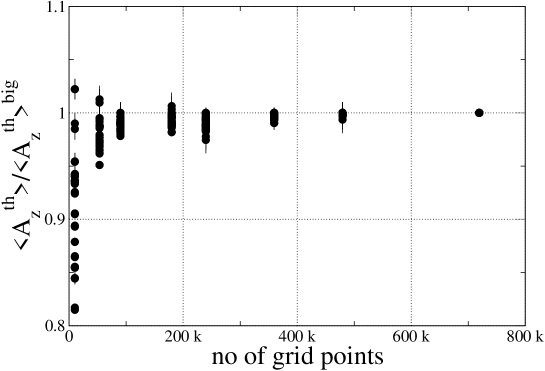
Figure 2: The ratio between the analyzing power $<A_{z}^{th}>$ calculated with grids with smaller numbers of grid points and the analyzing power $<A_{z}^{th}>^{big}$ obtained with the final, fine grid. The ratio of the two values is shown as a point for each of the 36 bins of the independent variable $\Delta\phi$.

To compare the (time-consuming) single-shot mode with the (fast) grid interpolation method, we have calculated the analyzing power $<A_{z}^{th}>$ as a function of $\Delta\phi$ using both methods. The values of $A^{th}_{z}$ for all events within a given $\Delta\phi$ bin are averaged according to Eq. (6) to give $<A_{z}>$ for that bin. The error bars are calculated according to Eq. (7) and turn out to be smaller than 0.003. The results from the single-shot mode (circles) and the grid interpolation method (crosses) are shown in Fig. 3a. The difference between the two results is shown in Fig. 3b. Again, this difference is a measure of the interpolation uncertainty, or, in other words, of the ’curvature’ of the interpolated function (hence the systematic dependence on $\Delta\phi$).

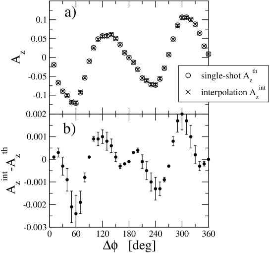
Figure 3: a) comparison of the single-shot calculation of $A^{th}_{z}$ (open circles) with the grid interpolation method $A^{int}_{z}$ (crosses); b) the difference between the two calculations

IV EXAMPLES

Recently, an experimental study of the $dp$ break-up reaction with polarized 270 MeV deuterons on a polarized proton target has been completed using the “Cooler” storage ring at the Indiana University Cyclotron Facility IUCFexp . In this section, we illustrate the use of our new method to obtain theoretical estimates of polarization observables for this experimental setup.

We calculated the differential cross section and several polarization observables $O^{th}(x)$ using the CD Bonn NN potential with and without the TM’ 3NF for each grid point in the available phase space. After that, using the multidimensional interpolation, cf. the appendix, we obtained theoretical predictions for each experimental phase space point (about $3*10^{6}$ experimental points). Using the averaging method of Eq. (6), the boundaries of the experimental acceptance for the energies and azimuths of the two outgoing protons, which are approximately $E_{1}^{lab},E_{2}^{lab}>50$ MeV, $10^{\circ}\leq\theta_{1}^{lab},\theta_{2}^{lab}\leq 45^{\circ}$, respectively, were automatically taken into account. The errors from the sampling statistics are obtained from Eq. (7).

The results for the vector analyzing power $A_{z}$, the tensor analyzing power $A_{zz}$ and the correlation coefficients $C_{zz,z}$, $C_{yx}-C_{xy}$ and $C_{xx}+C_{yy}$ are shown in Figs (4) - (6) as a function of $\Delta\phi$. In these figures the solid line shows the Faddeev calculations based on the CD Bonn NN potential, while the dashed line is obtained by including the TM’ 3NF. The errors (less than 0.003) are too small to be visible in figures.

The difference between the solid and the dashed lines illustrates the effect of the TM’ 3NF. As one can see, the 3NF effects are rather small in the present case where the observables are integrated over a large portion of the phase space. However, in the case of some correlation coefficients (Fig. 6) the magnitude of 3NF effects is sufficiently large to be distinguishable by a future experiment.

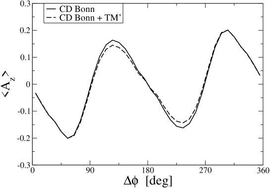
Figure 4: Average value of vector analyzing power as a function of $\Delta\phi$. The solid and dashed lines are the CD Bonn and CD Bonn + TM’ 3NF predictions, respectively.

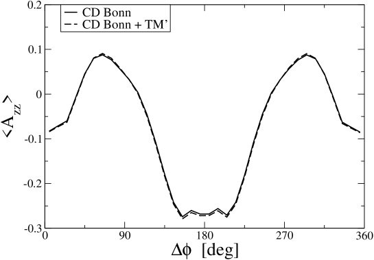
Figure 5: Average values of tensor analyzing power as a function of $\Delta\phi$. The solid and dashed lines are the CD Bonn and CD Bonn + TM’ 3NF predictions, respectively.

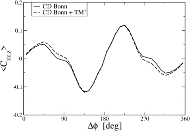
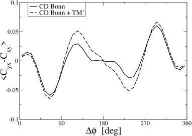
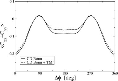
Figure 6: Average values of spin correlation coefficients as a function of $\Delta\phi$. The solid and dashed lines are the CD Bonn and CD Bonn + TM’ 3NF predictions, respectively.

It is conceivable that the smallness of the 3NF effects in some of the cases that are shown here is due to the fact the observable is averaged over a large portion of the phase space. In order to identify regions in phase space with strong 3NF effects, we have searched for the largest differences between observables predicted with the CD Bonn interaction either by itself, or with the TM’ 3NF included. The influence of the 3NF can be quantified by a difference $\Delta O^{th}$ at a given phase space point when the 3NF is switched on

$$\Delta O^{th}=|O^{th}(2N)-O^{th}(3N)|$$

Here $O^{th}(2N)$, $O^{th}(3N)$ are predictions for the particular observable resulting when using the CD Bonn potential alone and including in addition the TM’ 3NF, respectively.

First, for each observable $O^{th}$ we searched over the entire grid of the phase space points for the maximum value of the difference $\Delta O^{th}$. The results are presented in Table I. Second, since we are looking for the effects that should be experimentally accessible, we searched for the maximum of $\Delta O^{th}$ only through the phase space points for which the differential cross section $\frac{d\sigma}{d\hat{p}d\hat{q}dq}=\sigma(2N)>0.001\frac{fm^{2}}{MeVsr^{2}}$. The resulting $max[\Delta O^{th}]$ are shown in third column in Table I. In addition, in the brackets, labeled (*) and (**) of Table I, we list the number of grid points for which $0.05\leq\Delta O^{th}\leq max[\Delta O^{th}]$ and $0.05\leq\Delta O^{th}\leq max[\Delta O^{th}]$ with $\sigma(2N)>0.001\frac{fm^{2}}{MeVsr^{2}}$, respectively.

Table 1: Maximum value of difference $\Delta O^{th}=|O^{th}(2N)-O^{th}(3N)|$ for each observable $O^{th}$. The second column, labeled $max[\Delta O^{th}]$, gives results without any restrictions. The third one, labeled $max[\Delta O^{th}]+\sigma$, results after applying cross section limitation ( $\sigma(2N)>0.001\frac{fm^{2}}{MeVsr^{2}}$). In the brackets, in the column labeled (*), there is a number of grid points for which $0.05\leq\Delta O^{th}\leq max[\Delta O^{th}]$. In the column labeled (**) there are number of grid points for which $0.05\leq\Delta O^{th}\leq max[\Delta O^{th}]$ and $\sigma(2N)>0.001\frac{fm^{2}}{MeVsr^{2}}$.

$O^{th}$	$max[\Delta O^{th}]$	(*)	$max[\Delta O^{th}]+\sigma$	(**)
$A_{z}$	0.05	(10)		(0)
$A_{zz}$	0.12	(62 150)	0.12	(11 409)
$C_{xx}+C_{yy}$	0.18	(70 110)	0.11	(1 458)
$C_{yx}-C_{xy}$	0.08	( 4 350)		(0)
$C_{zz,z}$	0.10	( 2 376)		(0)

As we can see in Table I the tensor analyzing power $A_{zz}$ or the correlation coefficient $C_{xx}+C_{yy}$ are especially interesting, showing large 3NF effects, on the other hand the vector analyzing power $A_{z}$ shows the least evidence of the action of the TM’ 3NF.

The next step in our study was to find the regions of the phase space with the largest value of $\Delta O^{th}$. Let us investigate here, only for example, the dependence of $A_{zz}(\Delta\phi)$ on the additional variables $p$, $\theta_{p}$ and $\theta_{q}$. For this purpose, the four-dimensional phase space distributions of $<A_{zz}^{th}>$ and $\Delta A_{zz}^{th}$ are projected onto three planes: $\Delta\phi-p$, $\Delta\phi-\theta_{p}$ and $\Delta\phi-\theta_{q}$. In the case of $\Delta A_{zz}^{th}$ for each projection point the maximum value over the range of the remaining variables is determined, e.g. the $\Delta\phi-p$ projection shows $max[\Delta A_{zz}^{th}(p,\theta_{p},\theta_{q},\Delta\phi)]_{\Delta\phi,p}$.

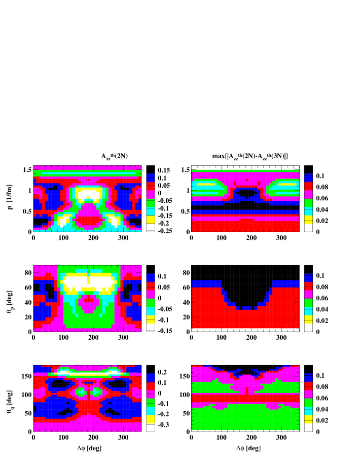
Figure 7: Two-dimensional projections of theoretical prediction for tensor analyzing power $A_{zz}^{th}$. Columns show the average value of $<A_{zz}^{th}(2N)>$ and the maximum of difference $|A_{zz}^{th}(2N)-A_{zz}^{th}(3N)|$. The three rows show projections onto the $\Delta\phi-p$, $\Delta\phi-\theta_{p}$ and $\Delta\phi-\theta_{q}$ planes, respectively.

Using graphs from the second column we can see which region of phase space exhibits a large 3NF effect. The figure shows, for example, that an interesting region would be $100^{\circ}\leq\theta_{q}\leq 180^{\circ}$ with the full range of $p$ and $\theta_{p}$ included. Fig. 8 shows the average value of $<A_{zz}^{th}>$ after integration over all values of $p$, $\theta_{p}$ and integration over part of $100^{\circ}\leq\theta_{q}\leq 180^{\circ}$. For this example the 3NF effects are quite large.

Studies such as this, together with earlier work published in  kuros03 , may be used to identify regions of enhanced sensitivity the the 3NF in order to plan future experiments.

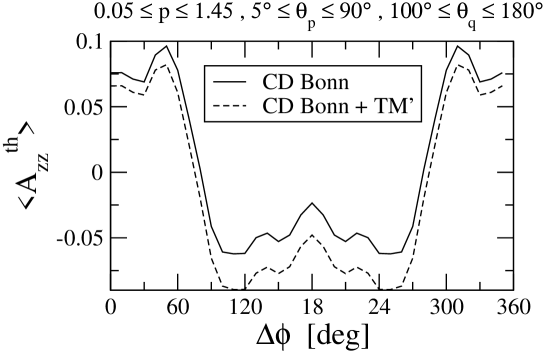
Figure 8: The average value of tensor analyzing power $A_{zz}$ as a function of $\Delta\phi$, in a region of phase space that is sensitive to the inclusion of a three-nucleon force ($0.05\leq p\leq 1.45,5^{\circ}\leq\theta_{p}\leq 90^{\circ},100^{\circ}\leq\theta_{q}\leq 180^{\circ}$). The solid and dashed lines are the CD Bonn and CD Bonn + TM’ 3NF predictions, respectively.

V SUMMARY

We have presented a simple, straight-forward method to integrate over regions of phase space the prediction from a theoretical model. The method reflects the true experimental acceptance, as well as variations of the detector efficiency. It is applicable to kinematically complete experiments with three bodies in the final state, and eliminates the need for a Monte-Carlo simulation of the detector setup.

We have applied this method to several observables of $dp$ break-up at 270 MeV, and studied the effect of including a three-nucleon force in the model.

Appendix A Multidimensional linear interpolation

The sampling method described in section II, requires that the theoretical value of a given observable is calculated for each of a large number of events, collected in an experiment. In order to achieve the necessary processing speed, precalculated theoretical values are stored in a four-dimensional matrix (the ’grid’) as explained in Sec. III.3. Multidimensional linear interpolation is then used to retrieve the corresponding value at any phase space point.

We denote the set of four continuous independent variables as $x=\{p,\theta_{p},\theta_{q},\Delta\phi\}\equiv\{x_{i}\}$; $(i=1..4)$. The corresponding discrete independent variables that constitute the grid are $x_{i,k_{i}}$, $k_{i}=1..n$, where $n$ is the size of the grid in the $i$th dimension. It is understood that $x_{i,k_{i}}\leq x_{i}\leq x_{i,k_{i}+1}$ for any value $x_{i}$ of the set $x$ at which a functional value is sought, i.e. the elements of the discrete grid $x_{i,k_{i}}$-variables are strictly increasing and the $x_{i}$ coordinate at which interpolation is performed lies always inside an interval of grid points. Applying linear interpolation bib:LinInt in four dimensions, means that the grid cell that contains the argument $x$ of interest has $2^{4}=16$ corners. We are using the FORTRAN routine FINT bib:FINT from the CERN program library. The interpolation is carried out as follows.

The interpolation weights, $w_{i}$, are defined as

$$w_{i}=\frac{x_{i}-x_{i,k_{i}}}{x_{i,k_{i}+1}-x_{i,k_{i}}}$$ (13)

For brevity we also define $u_{i}=1-w_{i}$. The functional values at the corners of the grid cell that contains $x$ are denoted by $y_{m}$; $m=1..16$, and defined as follows,

$$\begin{array}[]{l}y_{1}\equiv O(x_{1,k_{i}},x_{2,k_{i}},x_{3,k_{i}},x_{4,k_{i}})\\ y_{2}\equiv O(x_{1,k_{i}+1},x_{2,k_{i}},x_{3,k_{i}},x_{4,k_{i}})\\ y_{3}\equiv O(x_{1,k_{i}+1},x_{2,k_{i}+1},x_{3,k_{i}},x_{4,k_{i}})\\ y_{4}\equiv O(x_{1,k_{i}},x_{2,k_{i}+1},x_{3,k_{i}},x_{4,k_{i}})\\ y_{5}\equiv O(x_{1,k_{i}},x_{2,k_{i}},x_{3,k_{i}+1},x_{4,k_{i}})\\ y_{6}\equiv O(x_{1,k_{i}+1},x_{2,k_{i}},x_{3,k_{i}+1},x_{4,k_{i}})\\ y_{7}\equiv O(x_{1,k_{i}+1},x_{2,k_{i}+1},x_{3,k_{i}+1},x_{4,k_{i}})\\ y_{8}\equiv O(x_{1,k_{i}},x_{2,k_{i}+1},x_{3,k_{i}+1},x_{4,k_{i}})\\ ......\\ y_{16}\equiv O(x_{1,k_{i}},x_{2,k_{i}+1},x_{3,k_{i}+1},x_{4,k_{i}+1})\\ \end{array}$$ (14)

The observable at any point $x=(x_{1},x_{2},x_{3},x_{4},x_{5})$ is then given by

$$\begin{array}[]{l}O(x_{1},x_{2},x_{3},x_{4})=\\ u_{1}u_{2}u_{3}u_{4}\cdot y_{1}+w_{1}u_{2}u_{3}u_{4}\cdot y_{2}+w_{1}w_{2}u_{3}u_{4}\cdot y_{3}+u_{1}w_{2}u_{3}u_{4}\cdot y_{4}+\\ u_{1}u_{2}w_{3}u_{4}\cdot y_{5}+w_{1}u_{2}w_{3}u_{4}\cdot y_{6}+w_{1}w_{2}w_{3}u_{4}\cdot y_{7}+u_{1}w_{2}w_{3}u_{4}\cdot y_{8}+\\ u_{1}u_{2}u_{3}w_{4}\cdot y_{9}+w_{1}u_{2}u_{3}w_{4}\cdot y_{10}+w_{1}w_{2}u_{3}w_{4}\cdot y_{11}+u_{1}w_{2}u_{3}w_{4}\cdot y_{12}+\\ u_{1}u_{2}w_{3}w_{4}\cdot y_{13}+w_{1}u_{2}w_{3}w_{4}\cdot y_{14}+w_{1}w_{2}w_{3}w_{4}\cdot y_{15}+u_{1}w_{2}w_{3}w_{4}\cdot y_{16}\end{array}$$ (15)

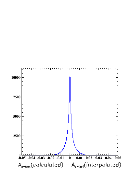
Figure 9: The difference between the interpolated and the exact test observable.

In order to investigate the accuracy of the interpolation routine, we construct a ’test’ grid that is analogous to the one described in Sec. III.3, but with function values that are given by the analytic expression

$$\begin{array}[]{l}O(x)=A_{z-test}(p,\theta_{p},\theta_{q},\phi_{p})=\\ 4{p}/{p_{max}}(1-{p}/{p_{max}})\cdot(\sin(\theta_{q})\sin(2\theta_{p})\sin(\phi_{p})+\sin 2(\theta_{q})\sin 2(\theta_{p})\sin(2\phi_{p}))\end{array}$$ (16)

where $p_{max}$ is the largest possible relative proton momentum. This function has been chosen to represent a possible, typical dependence of $A_{z}$ on the final-state kinematics.

For a large number of arguments $x$, corresponding to random, phase-space-distributed break-up events, the exact value of the function is compared to the value returned by the interpolation routine, acting on the grid values. The distribution of differences is shown in Fig. 9. The spread of values around zero arises because the interpolation assumes that the function is linear within a grid cell. This effect causes a systematic shift between the interpolated and the true values. For this reason, the FWHM of 0.003 observed in Fig. 9 should be compared to the value of the function. When averaging over regions of phase space this effect washes out further, becoming clearly insignificant indicating that the mesh size of the grid used here is sufficiently small.

References

- (1) C. R. Howell et al., Nucl. Phys. A631, 692 (1998); J. Strate et al., Nucl. Phys. A501, 51 (1989); H. Setze et al., Phys. Lett. B388, 299 (1996); G. Rauprich et al., Nucl. Phys. A535, 313 (1991); J. Zejma et al., Phys. Rev. C55, 42 (1997); K. Bodek et al., Few-Body Syst. 30, 65 (2001); M. Allet et al., Phys. Rev. C50, 602 (1996).
- (2) R. Machleidt, F. Sammarruca, and Y. Song, Phys. Rev. C53, R1483 (1996).
- (3) R. Machleidt, Phys. Rev. C63, 024001 (2001).
- (4) J. L. Friar, D. Hüber, U. van Kolck, Phys. Rev. C59, 53 (1999).
- (5) D. Hüber, J. L. Friar, A. Nogga, H. Witała, U. van Kolck, Few-Body Syst. 30, 95 (2001).
- (6) Polarization Observables in d+p Break-up at 270 MeV, T.J. Whitaker, Ph.D. thesis, IUCF, 2004.
- (7) W. Glöckle, H. Witała, D. Hüber, H. Kamada and J. Golak, Phys. Rep. 274, 107 (1996).
- (8) D. Hüber, H. Kamada H. Witała, W. Glöckle, Acta Phys. Pol. B 28, 1677 (1997).
- (9) G. O. Ohlsen, Rep. Prog. Phys. 35 (1972) 717.
- (10) W. H. Press, S. A. Teukolsky, W. T. Vetterling, B. P. Flannery, ’Numerical Recipes’, Cambridge Press, Cambridge, 1996.
- (11) J. Kuroś-Żołnierczuk et al., Phys. Rev. C66, 024003 (2002).
- (12) http://wwwinfo.cern.ch/asdoc/shortwrupsdir/e104/top.html