Nuclear halo and its scaling laws

Abstract

We have proposed a procedure to extract the probability for valence particle being out of the binding potential from the measured nuclear asymptotic normalization coefficients. With this procedure, available data regarding the nuclear halo candidates are systematically analyzed and a number of halo nuclei are comfirmed. Based on these results we have got a much relaxed condition for nuclear halo occurrence. Furthermore, we have presented the scaling laws for the dimensionless quantity $<r^{2}>/R^{2}$ of nuclear halo in terms of the analytical expressions of the expectation value for the operator $r^{2}$ in a finite square-well potential.

Date text]May 29, 2003

1. INTRODUCTION

Nuclear halo is a threshold phenomenonrefHa95 . As the binding energy becomes small, the wave function of valence particle extends more and more outward if the centrifugal barrier is small ($l\leq 1$). Eventually, this leads to the wave function penetrating substantially beyond the range of nuclear force as the binding energy approches zero, i.e., occurrence of nuclear halo.

The occurrence conditions for nuclear halo have already been discussed in detail in the literaturerefRi92 ; refFe93 ; refFe94 ; refJe00 . Jensen and RiisagerrefJe00 , recently, proposed the necessary conditions,

$$B_{p}<270\frac{A^{2}}{Z^{2}}\text{ keV \thinspace\thinspace\thinspace for s-states,}$$ (1)

$$Z<0.44A^{4/3}\text{ \thinspace\thinspace\thinspace\thinspace for p-states,}$$ (2)

$$B_{p}<2A^{-2/3}\text{ MeV \thinspace\thinspace\thinspace for both s- and p-states,}$$ (3)

where $B_{p}$ is the binding energy of valence particle. Eq.(3) overrules Eq.(1) and becomes decisive for all $A$ for s-states as they pointed out. Most of halo nuclei experimentally observerd as well as theoretically predicted are s-wave halo. Hence, Eq.(3) is the most important conditions for halo occurrence.

Among the nuclear halo candidates, however, only the well-known s-wave halos in ${}^{11}Li$, ${}^{11}Be$ and the p-wave halo in ${}^{11}Be$ with the $B_{p}A^{2/3}$ values of $1.48$ $MeV$, $2.49$ $MeV$ and $0.89$ $MeV$, respectively, are below or close to the limit set by Eq.(3). As will be seen , the others have binding energies much larger than this requirement. Therefore, it might be necessary to make a systematic inquiry concerning the occurrence conditions and scaling laws of nuclear halo. To this end, we have first to select, if possible, a proper experimental observable which can be employed to characterize the spatial extension of valence particle density. Direct measurements of the nucleonic density distribution should provide a visualized picture of nuclear skin and halo stuctures, therefore will be very interesting. Over the years a large variety of experimental methods have been developed, using leptonic probs (as electrons, muons, etc.) for investigating nuclear charge distributions, and hadronic probs (as protons, $\alpha-$particles, pions, etc.) for exploring the distributions of nuclear matter refEg02 . All these methods were applied successfully for many years for the study of stable nuclei. Nowadays, study on the structures of exotic nuclei with many possible methods has become a new and exciting field of research. Recently, proton-nucleus elastic scattering at intermediate energies was applied for obtaining accurate and detailed information on the size and radial shape of halo nuclei refAl97 . Instead of density distribution, the probability of a valence particle being out of the binding potential may be a suitable quantity to assess the degree of the spatial extension. In the following, we will present a procedure to extract the probability from experimental data in a more reliable way, and try to get the occurrence conditions and scaling laws of nuclear halo, which might be in line with experimental observations. In this paper, we will limit ourselves to an investigation on two-body nuclear halos.

2. PROBABILITY OF VALENCE PARTICLE BEING OUT OF THE BINDING POTENTIAL

The probability for valence particle being out of the binding potential radius $R$ can be evaluated by,

$$P(R,r_{0},a_{0})=\frac{\int_{R}^{\infty}r^{2}\phi_{nlj}^{2}(r)dr}{\int_{0}^{\infty}r^{2}\phi_{nlj}^{2}(r)dr}\text{,}$$ (4)

where $\phi_{nlj\text{ }}$represents the normalized sigle-particle radial wave function in the ($nlj$) bound state, $r_{0}$ and $a_{0}$ are the radius and diffuseness parameters of the potential,and the binding potential radius $R$ is a equivalent square-well potential radius which can be derived from the measured mean-square core radius by $R^{2}=\frac{5}{3}\left(<r^{2}>_{c}+4\right)$ $fm^{2}$ refFe93 ; refRi00 . We have explicitly indicated the dependence of the probability $P$ on $R$, $r_{0}$ and $a_{0}$. At the asymptotic distance $\phi_{nlj}$ behaves like,

$$\phi_{nlj}\simeq b_{lj}\frac{W_{-\eta,l+1/2}(2kr)}{r},$$ (5)

where $W_{-\eta,\text{ }l+1/2}(r)$ is the Whittaker function, $k=\sqrt{2\mu B_{p}/\hslash^{2}}$ is the wave number, and $\mu$ and $\eta$ are the reduced mass and the Coulomb parameter for system $\left(A_{c}+N\right)$. In the neutron case where $\eta=0$, Whittaker function is related to the modified Bessel function $K_{l+1/2}(kr)$ as $W_{0,l+1/2}(2kr)=\sqrt{kr/\pi}K$ ${}_{l+1/2}(kr)$refAb70 . In Eq. (5), $b_{lj}$ is the single-particle asymptotic normalization coefficient ($ANC$) defining the amplitude of the single-particle wave function in the asymptotic region. The single-particle $ANC$ and the single-particle spectoscopic factor $S_{lj}^{(sp)}$ are related to the nuclear $ANC,C_{A_{c}Nlj}^{A},$ byrefMu01 ,

$$C_{A_{c}Nlj}^{A}=b_{lj}(S_{lj}^{(sp)})^{1/2}\text{.}$$ (6)

for virtual process $A\rightleftarrows A_{c}+N$. Here $A,$ $A_{c}$ and $N$ stand for the nucleus, its core nucleus and the valence particle, respectively. Nuclear $ANC$ is an experimentally measurable and independent of parameters of the potential refMu01 ; refLiu01 .

The probability calculated with Eq.(4) is only theoretical value and potential-parameter dependent. Eq. (6) sets a restraint on the single-particle wave function $\phi_{nlj}(r).$The amplitude of $\phi_{nlj}(r)$ at the asymptotic distances, $b_{lj}$, is fixed as long as the values of $C_{A_{c}Nlj}^{A}$ and $S_{lj}^{(sp)}$ are given. However, the potential parameters $r_{0}$ and $a_{0},$ hence the single-particle wave functions are not determined uniquely. We search the potential parameters in such a way that the quantity,

$$\chi_{p}^{2}=\sum_{r_{i}=R_{N}}^{40fm}\left(S_{lj}^{1/2}\phi_{nlj}\left(r_{i}\right)-C_{A_{c}Nlj}^{A}\frac{W_{-\eta,l+1/2}\left(2kr_{i}\right)}{r_{i}}\right)^{2}$$ (7)

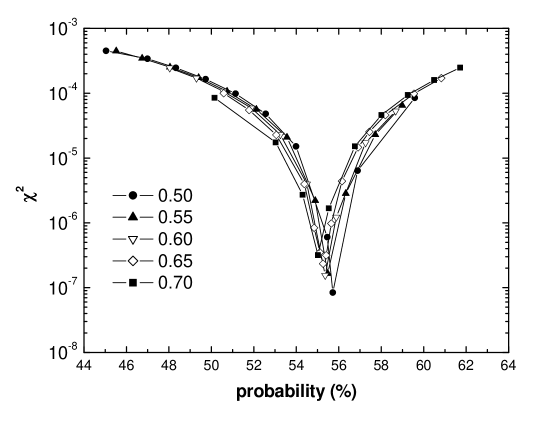
Figure 1: Dependence of the $\chi_{p}^{2}$ on the probability for valence particle being out of the binding potential $P$ for the $2s$ excited state in ${}^{13}C$. Symbols are connected by a line for each $a_{0}$ value to guide the eye.

becomes minimum. This is because $\phi_{nlj}(r)$ has the asymptotic behaviour specified by Eq. (5) and Eq. (6) when $\chi_{p}^{2}$ turns into minimum. We extract the probability from the experimental data of $C_{A_{c}Nlj}^{A}$ and $S_{lj}^{(sp)}$ as follows. First, single-particle wave function is calculated with the Woods-Saxon potential. The depth of the potential is adjusted to reproduce the binding energy $B_{p}$. The values of diffuseness parameter $a_{0}$ are choosen in the range of $0.50-0.70$ fm. For each fixed $a_{0}$ , the radius parameter $r_{0}$ is varied in a small step till the minimum in $\chi_{p}^{2}$ is reached. In the calculation of $\chi_{p}^{2}$, the summation runs from $r_{i}=6.0$ fm to 40 fm in step of 0.1 fm . We find that the value of $\chi_{p}^{2}$ does not change as long as $R_{N}\geq 6$ fm. Then, for each pair of $\left(r_{0},a_{0}\right)$ the probability for the valence particle being out of the binding potential radius R is calculated with Eq. (4). Alternatively, one may take the radius, $R_{ws}=r_{0}A_{c}^{1/3\,}[1+5/3(\pi a_{0}/(r_{0}A_{c}^{1/3\,}))^{2}]^{1/2\,}$refFe94 , as binding potential radius instead of $R$. We find that the value of $R$ and the values of $R_{ws}$ at the minima in $\chi_{p}^{2}$  are nearly the same. Hence, the probabilities calculated with Eq. (8) below are nearly identical whether $R$ or $R_{ws}$ is used. Besides, the results are the same within the experimental error when $S_{lj}^{(sp)}$ changes 10%. Because the relative uncertainty of the experimental $S_{lj}^{(sp)}$ is usually less than 10%, therefore, the results below are reliable within the accuracy of  $S_{lj}^{(sp)}$. Figure 1 shows the $\chi_{p}^{2}$ as a function of the probability $P$ for the $2s$ excited state in ${}^{13}C$. In this calculation, $C_{A_{c}Nlj}^{A}=1.84\pm 0.16fm^{-1/2}$ refLiu01 and  $S_{lj}^{(sp)}=0.95$ refJa83 are used. It can be seen from the figure that the minimum in $\chi_{p}^{2}$ is very deep with a very small dispersion in the probability $P$. This is actually due to the fact that $\chi_{p}^{2}$ reaches its minimum value when Eq. (6) is satisfied. Therefore, in terms of the experimentally measured nuclear asymptotic normalization coefficients $C_{A_{c}Nlj}^{A}$, we can calculate the average value of the probability $P$ by,

$$P=\sum w_{i}P(R,r_{0i},a_{0i})\text{,}$$ (8)

with

$$w_{i}=\frac{(\chi_{p}^{2}\left(r_{0i},a_{0i}\right))^{-1}}{\sum\left(\chi_{p}^{2}\left(r_{0i},a_{0i}\right)\right)^{-1}}\text{.}$$ (9)

The summation runs over the minimum points in $\chi_{p}^{2}$ for different $a_{0}$. It is worth to note that the probability obtained in this way is nearly parameter independent. This is an interesting and meaningful result within the reach of present experimental knowledge.

By means of the above procedure, the probability for the valence particle being out of the binding potential have been calculated for a number of nuclei. The values listed in Table 1 are the weighted average probability $P$ extracted from different experimental sources. The results are plotted in Figs. 2(a) and (b) as a function of $2\mu B_{p}R^{2}/\hbar^{2}$ and $B_{p}A^{2/3}$, respectively. Riisager et al.refRi94 ; refHa95 ; refJe00 suggest a criterion for quantitative assessment of halos, i.e., the valence particle has large probability, say ¿ 50%, of being out of the nuclear binding potential radius. According to this criterion, the nuclei under considerations are all s-wave halo in the ground state (solid points) or in the excited states (open circles). We find from Fig. 2(b) that halo may be able to occure for

$$B_{p}A^{2/3}<10\text{ }MeV$$ (10)

which is much relexed than the one given by Eq. (3).

We have calculated the probability for the valence neutron in 2s-state using Woods-Saxon potential with normal parameters $r_{0}=1.27$ $fm,$  $a_{0}=0.67$ $fm$, $U_{0}=\left(50-32\frac{N-Z}{A}\right)$ $MeV$ for the nuclei with $N=Z$ and $(N-Z)/A=1/3$, respectively. The binding potential radius $R$ used here is also calculated by $R^{2}=\frac{5}{3}\left(<r^{2}>_{c}+4\right)$ $fm^{2}$ and $<r^{2}>_{c}=(r_{0c}A^{1/3})^{2}$ ,the $r_{0c}$ is obtained by fitting to the experimental $rms$ radii of light nuclei.The calculated results are also plotted in Fig. 2 as the solid and dashed lines. Basically, they are in agreement with the experimental data. In order to examine the effects of larger diffuseness, we have plotted in Fig. 2(a) the probabilities for the Woods-Saxon potential with the same parameters as those used above except for doubling the diffuseness, $a_{0}=1.34$ $fm$. As shown by the dash-dotted and dotted lines, these calculations overpredict the experimental data. It means that using a very large diffuseness in potential may not correspond to the realistic situation for nuclei with weakly bound neutrons.

The probability of a valence particle being out of the square-well potential is,

$$P=\frac{1}{\chi+1}\left(1-\frac{\chi^{2}}{\xi_{0}^{2}}\right)\text{ \ \ }l=0,$$ (11)

$$P=\frac{\chi+2}{\chi^{2}+3\chi+3}\left(1-\frac{\chi^{2}}{\xi_{0}^{2}}\right)\text{ \ \ }l=1.$$ (12)

For $l$=$2$,

$$P=\frac{\chi^{3}+6\chi^{2}+12\chi+6}{(\chi+1)(\chi^{3}+6\chi^{2}+15\chi+15)}(1-\frac{\chi^{2}}{\xi_{0}^{2}})\rightarrow 0.4\text{ \thinspace\thinspace\thinspace\thinspace}(\chi\rightarrow 0),$$ (13)

where

$$\chi=R\sqrt{\frac{2\mu B_{p}}{\hbar^{2}}},$$ (14)

and

$$\xi_{0}=R\sqrt{\frac{2\mu U_{sq}}{\hbar^{2}}}.$$ (15)

In the above equations, $U_{sq}$ is the depth of the square-well potential. The dash-double-dotted line in Fig. 2(a) illustrats the square-well potential predictions for 2s-state. We see that it underpredicts the experimentally extracted data, implying the important roles of the potential diffuseness on the probability being out of the binding potential radius.

3. SCALING LAWS OF TWO-BODY NUCLEAR HALO

In terms of nuclear $ANC,$ we can extract the root-mean-square $\left(rms\right)$ radius of the probability distribution for valence particle in the orbit $\left(nlj\right)$. It can be written as the contributions from the interior and asymptotic regions refLiu01 ; refCa01 ,

$$<r^{2}>^{1/2}=\left[S_{lj}\int_{0}^{R}r^{4}\phi_{nlj}^{2}(r)dr+\left(C_{A_{c}Nlj}^{A}\right)^{2}\int_{R}^{\infty}r^{2}W_{-\eta,\text{ }l+1/2}^{2}\left(2kr\right)dr\right]^{1/2}.$$ (16)

The first term in the equation is somehow parameter dependent, while the second term is not. Moreover, in the case of weakly bound nuclei, the second term gives more than 90% contribution to the value of the $rms$ radius. Thus the error introduced by the parameters is small in the cases under consideration. The $rms$ radii of the valence particle have been calculated in this way for the nuclei ¹¹Be refOz01 ; refAj90 ; refFo99 ; refAu00 , ¹²B refLiu01 , ^13,14,15C refLiu01 ; refOz01 ; refLiu02 ; refAj91 , ${}^{19}C$ refOz01 ; refBa00 . They are listed in Table 1 along with other parameters. Based on the assumption of a core plus a valence neutron structure, recently, Ozawa et al. refOz01 applied a Glauber-model analysis for a few body system $\left(GMFB\right)$, and deduced spectroscopic factors $S_{lj}$ for some selected nuclei from the measured interaction cross sections $\sigma_{I}$. With their parameters of the binding potential, we calculate the single-particle wave function and obtain single-particle $ANC$ $b_{lj}$ in asymptotic region. Then, the nuclear $ANC$ can be obtained from the deduced $S$-factor and the single-particle $ANC$ $b_{lj}$ with Eq. (6). The $rms$ radii for ¹¹Be$,^{15,19}$C are evaluated by means of the $GMFB$ analysis, and the results are also listed in Table 1. In order to check the above results, the $rms$ radii of the valence particle wave functions in these three nuclei are extracted by subtracting the core contribution from the mean-square matter radius refRi00 :

$$<r^{2}>=\frac{A^{2}}{A_{c}A_{h}}<r^{2}>_{m}-\frac{A}{A_{h}}<r^{2}>_{c},$$ (17)

where $A$, $A_{c}$ and $A_{h}$ are the total, core and valence particle mass numbers of the system, respectively. These $rms$ radii are compared with the other data in Table 1. Except for ¹⁵C, the $rms$ radii of halo obtained with these three methods are in agreement within the experimental errors.

Hamamoto and ZhangrefHa98 have deduced the expressions for the expectation value of the operator $r^{2}$ in a finite square-well potential. The terms with $\xi_{0}^{4\text{ }}$in denominator in thier expressions are negligible in magnitude as compared to the other terms for the case of $\chi^{2}<2$ which we are interested in. After omitting them, we get the following scaling laws,

$$\frac{<r^{2}>}{R^{2}}=\frac{1}{\chi+1}\left[\left(1-\frac{\chi^{2}}{\xi_{0}^{2}}\right)(1+\frac{1}{\chi}+\frac{1}{2\chi^{2}})+\chi(\frac{1}{3}+\frac{1}{2\xi_{0}^{2}}+\frac{\chi}{\xi_{0}^{2}})\right]\text{ \ \ }l=0,$$ (18)

$$\frac{<r^{2}>}{R^{2}}=\frac{1}{\chi^{2}+3\chi+3}\left[\left(1-\frac{\chi^{2}}{\xi_{0}^{2}}\right)\left(\frac{(\chi+1)^{2}}{3}+\chi+3+\frac{5}{2\chi}\right)+\frac{(\chi+1)^{2}}{2\xi_{0}^{2}}\right]+\frac{\left(\chi^{2}+2\chi+2\right)}{3\xi_{0}^{2}}\text{ \ \ }l=1$$ (19)

Keeping the largest term of the above eqations in the limit $\chi\rightarrow 0$, we will arrive at the scaling laws in Ref.refFe93 . It should be kept in mind that the above laws depend on the quantum number $n$ through $\xi_{0}$. Here $n$ is the node number of the radial wave function of valence particle. If halo is defined in terms of the requirement that the experimental value of probability $P$ is greater than 50%, or approximatelly $\chi^{2}\leq 1.8$ (see Fig.2(a)) ,we get the following conditions from Eqs. (18) and (19) for nuclear halo occurrence,

$$\frac{<r^{2}>}{R^{2}}\geq 1.5\text{ \ \ for }2s\text{ states,}$$ (20)

$$\frac{<r^{2}>}{R^{2}}\geq 1.9\text{ \ \ for }1p\text{ states.}$$ (21)

Since the probability $P$ is less than 40% for $l=2$, we come to the same conclusion as Riisager et al refRi92 that halo is unlikely to occur for the particle in the $d$ states.

In Fig. 3, the experimental data of $<r^{2}>/R^{2}$ are compared with our scaling law as well as the predictions of the single-particle model for the valence particle in $2s$ state. In order to have a better statistics, we adopt the weighted average value of $<r^{2}>$ instead of the individual experimental results. For the data without error, we assigned them to 10% of uncertainty for evaluating the weighted average.We see from the figure that the scaling law Eq. (18) can account for the available experimental data of halo candidates,though it is derived in a finite square-well potential. Several authors refRi00 ; refFe93 ; refHa87 ; refJe01 have put forward their scaling laws. Being of their $l$ and/or $n$ independent, we  do not present them in the figure.

4. SUMARRY

In summary, we have proposed a procedure to extract the probability for valence particle being out of the binding potential from the measured nuclear asymptotic normalization coefficients. With this procedure, available data regarding the nuclear halo candidates are systematically analyzed and a number of halo nuclei are comfirmed. Based on these results we have got a much relaxed condition for nuclear halo formation as compared to Ref.refJe00 . The effect of potential deffuseness on the probability being out of the nuclear binding potential radius is also discussed. In terms of the analytical expressions of the expectation value for the operator $r^{2}$ in a finite square-well potential, we have presented the scaling laws for the dimensionless quantity $<r^{2}>/R^{2}$ of nuclear halo,which can account for the available experimental data of halo candidates.

Table 1: Deduced nuclear $ANC$, $probability$, $rms$ radii and $<r^{2}>/R^{2}$ for the nuclear halo candidates.

Nucleus	$J^{\pi}$	$B_{p}$	$C_{ANlj}^{B}$	$probability$	$<r^{2}>^{1/2}$	$<r^{2}>_{av}^{1/2}$	$<r^{2}>_{av}/R^{2}$	Ref.
		$\left(keV\right)$	$\left(fm^{-1/2}\right)$	$(\%)$	$\left(fm\right)$	$\left(fm\right)$
${}^{11}Be$	$1/2^{+}$	504	0.81$\pm$0.05	-	6.68$\pm$0.43a	-	-	refOz01
			-	-	6.65$\pm$0.31b	-	-	refOz01
			0.76$\pm$0.03	-	6.23$\pm$0.25	-	-	refAj90
			0.78	-	6.40	-	-	refAj90
			0.81	-	6.68	-	-	refFo99
			0.78	-	6.44	-	-	refAu00
			-	78.6$\pm$7.5	-	6.46$\pm$0.16	2.60$\pm$0.13
${}^{12}B$	$1^{-}$	749	0.94$\pm$0.08	68.5$\pm$11.7	5.64$\pm$0.90	5.64$\pm$0.90	1.86$\pm$0.60	refLiu01
	$2^{-}$	1696	1.34$\pm$0.12	54.2$\pm$4.0	4.01$\pm$0.61	4.01$\pm$0.61	1.10$\pm$0.31	refLiu01
${}^{13}C$	$1/2^{+}$	1857	1.84$\pm$0.16	55.5$\pm$9.6	5.04$\pm$0.75	5.04$\pm$0.75	1.55$\pm$0.47	refLiu01
${}^{14}C$	$0^{-}$	1274	1.54$\pm$0.09	64.0$\pm$7.5	5.78$\pm$0.36	5.78$\pm$0.36	1.97$\pm$0.26	refLiu02
	$1^{-}$	2083	1.84$\pm$0.11	56.1$\pm$6.7	4.57$\pm$0.30	4.57$\pm$0.30	1.34$\pm$0.18	refLiu02
${}^{15}C$	$1/2^{+}$	1218	1.05$\pm$0.22	-	3.65$\pm$0.82a	-	-	refOz01
			-	-	4.59$\pm$1.02b	-	-	refOz01
			1.40	-	5.40	-	-	refAj91
			1.49$\pm$0.15	-	5.86$\pm$0.60	-	-	refLiu02
			-	60.4$\pm$6.6	-	5.15$\pm$0.34	1.55$\pm$0.21
${}^{19}C$	-	240	0.57$\pm$0.19	-	7.87$\pm$1.49a	-	-	refOz01
			-	-	7.63$\pm$2.46b	-	-	refOz01
			0.55$\pm$0.07	-	7.07$\pm$0.50	-	-	refBa00
			-	80.8$\pm$19.9	-	7.17$\pm$0.47	2.58$\pm$0.34

^a Deduced with GMFB method.   ^b Calculated with Eq. 17.           

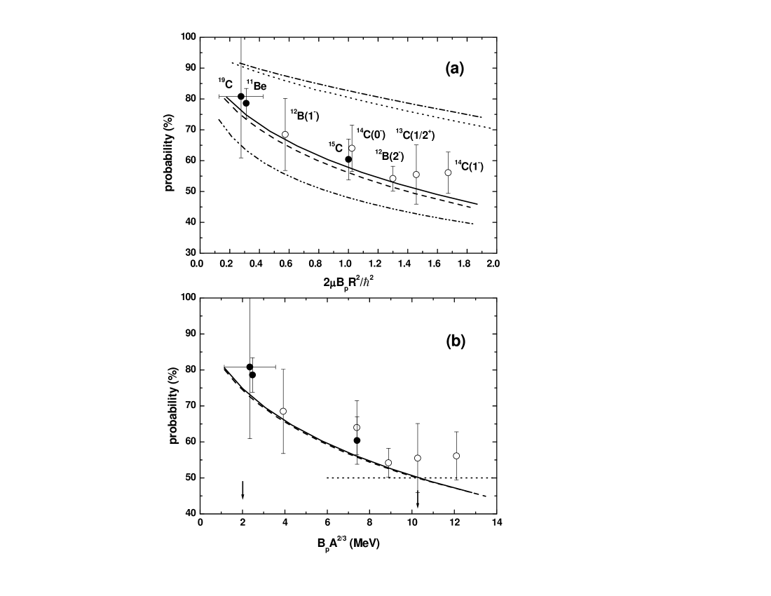
Figure 2: Probability for valence particle being out of the binding potential as a function of $2\mu B_{p}R^{2}/\hbar^{2}$ (a) and $B_{p}A^{2/3}$ (b). The solid points and open circles represent the $s$-wave halos in the ground state and in the excited states, respectively. The lines show the predictions of the single-particle models with Woods-Saxon potentials and the square-well potential. The arrows in the panel (b) illustrate the up-limits of $B_{p}A^{2/3}$ value set by Eq. (3), and Eq. (10).

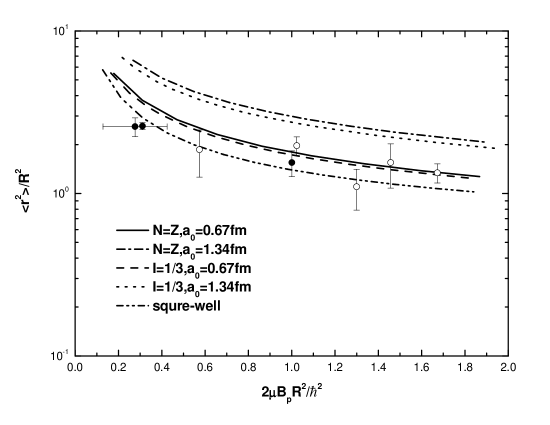
Figure 3: Experimental data of $<r^{2}>/R^{2}$ vs $2\mu B_{p}R^{2}/\hbar^{2}$ for the valence particle in the $2s$ state. The dash-double-dotted line is the scaling law of Eq. (18). The other lines show the results of the single-particle model calculations with Woods-Saxon potentials for the nuclei with N=Z and I=(N-Z)/A=1/3, respectively.