The Operator form of ³H (³He) and its Spin Structure

Abstract

An operator form of the 3N bound state is proposed. It consists of eight operators formed out of scalar products in relative momentum and spin vectors, which are applied on a pure 3N spin 1/2 state. Each of the operators is associated with a scalar function depending only on the magnitudes of the two relative momenta and the angle between them. The connection between the standard partial wave decomposition of the 3N bound state and the operator form is established, and the decomposition of these scalar function in terms of partial wave components and analytically known auxiliary functions is given. That newly established operator form of the 3N bound state exhibits the dominant angular and spin dependence analytically. The scalar functions are tabulated and can be downloaded. As an application the spin dependent nucleon momentum distribution in a polarized 3N bound state is calculated to illustrate the use of the new form of the 3N bound state.

I Introduction

Today it can be considered as standard to solve the Schrödinger equation for three nucleons numerically with high precision. This can be done either in the form of Faddeev equations Nogga et al. (2000, 2002), using hyperspherical expansion A. Kievsky et al. (1993); A. Kievsky (1997) or the Gaussian-basis method Kamimura (1988). Also the Greens-Function-Monte-Carlo (GFMC) and No-Core-Shell Model approaches have been applied to the three nucleon system Pieper and Wiringa (2001); P. Navrátil and B. R. Barrett (1998). These methods except for GFMC have always been based on standard partial wave expansions. Only recently for the study of three bound bosons the Faddeev equation has been solved directly in terms of relative momentum vectors Elster et al. (1999); Liu et al. (2002, 2003). Though any expectation value for a three-nucleon (3N) bound state can be determined numerically from wave functions obtained by any of the above mentioned methods, no analytic insight can be extracted for the spin and momentum (or configuration) dependence of the 3N bound state.

For the deuteron Rarita and Schwinger Rarita and Schwinger (1941a, b) introduced an operator form of the deuteron state in terms of spin operators and the relative position vector. This representation is ideal to exhibit the probabilities for finding any spin orientations in relation with the relative position (or momentum) vectors of the two nucleon in a polarized deuteron. In the case of a momentum representation of the deuteron derived from modern nucleon-nucleon (NN) forces this is illustrated in Ref. Fachruddin et al. (2001) and for a coordinate representation in Ref. Forest et al. (1996).

For three nucleons it is much more difficult to express the spin and momentum dependence of the bound state in an analytic form. Again, this analytic form has been worked out long time ago by Gerjuoy and Schwinger Gerjuoy and Schwinger (1942). For the 3N bound state, however, the functions multiplying the different scalars built from spin and position vectors depend on three variables, namely the magnitudes of the Jacobi vectors and the angle between them. In Ref. Gerjuoy and Schwinger (1942) the wave function is expanded in nine operators with nine corresponding scalar functions, which were numerically unknown in those days. It is the aim of this paper to establish an analytic link between these functions and the usual partial wave representation of the 3N bound state. This will lead to an alternative representation of the ³H (³He) bound states, which is more accessible to analytic insights into the spin structure of the 3N bound state. In our analysis we also find that the last term given in Ref. Gerjuoy and Schwinger (1942) is redundant, further simplifying this representation.

The paper is organized as follows. In Section II we start from the standard partial wave representation of the 3N bound state and reformulate it in terms of scalar operators acting on pure spin states with the correct spin quantum numbers of ³H (³He). This reformulation then leads at the same time to the scalar functions. Section III is devoted to the numerical investigation of the scalar functions. In Section IV we give an example for the application of the operator form of the ³He wave function and evaluate the probability to find a neutron with given momentum vector and polarized in the direction of the overall polarization of ³He. Several appendices include technical steps for the derivations. Finally we summarize in Section V.

II The Operator Form of the ³H (³He) Bound State

II.1 Derivation

The starting point for the derivation of an operator form is the standard partial wave representation of a 3N bound state. Here we do not use the isospin formalism and choose particles $1$ and $2$ to be neutrons(protons) and particle $3$ to be the proton(neutron). For the derivation we will assume a ³H bound state, but the generalization to ³He is obvious. In momentum space the 3N bound state with total angular momentum $1/2$ and magnetic quantum number $m$ can be written as

$$\Psi^{m}({\bf p},{\bf q}) \equiv \langle{\bf p}{\bf q}|\Psi^{m}\rangle$$ (1)

$$= \sum_{sSM_{S}}|(s\frac{1}{2})SM_{S}\rangle\langle(s\frac{1}{2})SM_{S}|\langle{\bf p}{\bf q}|\Psi^{m}\rangle$$

$$= \sum_{sSM_{S}}|(s\frac{1}{2})SM_{S}\rangle\sum_{l\lambda L}C(LS\frac{1}{2},m-M_{S}\>M_{S}){\mathcal{Y}}^{Lm-M_{S}}_{l\lambda}({\hat{\bf p}}{\hat{\bf q}})\>\Psi_{l\lambda LsS}(pq)$$

$$= \sum_{sS}\sum_{l\lambda L}\left[{\mathcal{Y}}^{L}_{l\lambda}({\hat{\bf p}}{\hat{\bf q}})|(s\frac{1}{2})S\rangle\right]^{\frac{1}{2}m}\>\Psi_{l\lambda LsS}(pq),$$

where ${\bf p}$ and ${\bf q}$ are the standard Jacobi momenta Glöckle (1983), and the ${\hat{\bf p}}$ and ${\hat{\bf q}}$ stand for the corresponding unit vectors. The 3N spin state $|(s\frac{1}{2})SM_{S}\rangle$ is constructed by coupling the spin state of the two neutrons with total spin $s$ and the spin of the proton $(\frac{1}{2})$ to the total spin $S$ and magnetic quantum number $M_{S}$ of the 3N system. Furthermore, $l$, $\lambda$, and $L$ are the relative orbital angular momenta of the two neutrons (related to ${\bf p}$), the orbital angular momentum of the proton (related to ${\bf q}$) and the total orbital angular momentum of the three nucleons. The bracket in the last equation is a convenient abbreviation for the LS-coupling employed here. The quantities $\Psi_{l\lambda LsS}(pq)$ represent the partial wave components of the 3N bound state. They are for example determined by the solution of the Faddeev equations Nogga et al. (2000, 2002). Typical numbers for a good representation of $\Psi^{m}({\bf p},{\bf q})$ are $l\leq 3$, $\lambda\leq 3$. The wave function is antisymmetric in the two neutrons, which constrains $l+s$ to be even. Note that we solve the Schrödinger equation using the isospin formalism. The particle basis wave functions, which enter in Eq. (1), are a combination of total isospin $T=1/2$ and $T=3/2$ wave functions, namely

$$\Psi_{l\lambda LsS}(pq)=\sqrt{3}\ \left(\ (-)^{M_{T}+3/2}\ \sqrt{2\over 3}\ \Psi_{l\lambda LsS}^{t=1\ T={1\over 2}}(pq)+\sqrt{1\over 3}\ \Psi_{l\lambda LsS}^{t=1\ T={3\over 2}}(pq)\right)$$ (2)

where $M_{T}$ is the third component of the isospin, namely $M_{T}=1/2$ for ³He and $-1/2$ for ³H. Note that the isospin of the neutron-neutron or proton-proton two-body subsystem is restricted to $t=1$. The overall factor $\sqrt{3}$ is a consequence of the identity of the nucleons in the isospin formalism and insures the correct normalization.

The right hand side of Eq. (1) naturally decomposes into four parts according to the total spin $S=1/2$ or $S=3/2$ and the total orbital angular momentum $L=0,1$, and $2$ as

$$\Psi^{m}({\bf p},{\bf q}) = \sum_{s}\sum_{l}\left[{\mathcal{Y}}^{0}_{ll}({\hat{\bf p}}{\hat{\bf q}})\mid(s\frac{1}{2})\frac{1}{2}\rangle\right]^{\frac{1}{2}m}\>\Psi_{ll0s\frac{1}{2}}(pq)$$ (3)

$$+\sum_{s}\sum_{l\lambda}\left[{\mathcal{Y}}^{1}_{l\lambda}({\hat{\bf p}}{\hat{\bf q}})\mid(s\frac{1}{2})\frac{1}{2}\rangle\right]^{\frac{1}{2}m}\>\Psi_{l\lambda 1s\frac{1}{2}}(pq)$$

$$+\sum_{l\lambda}\left[{\mathcal{Y}}^{1}_{l\lambda}({\hat{\bf p}}{\hat{\bf q}})\mid(1\frac{1}{2})\frac{3}{2}\rangle\right]^{\frac{1}{2}m}\>\Psi_{l\lambda 11\frac{3}{2}}(pq)$$

$$+\sum_{l\lambda}\left[{\mathcal{Y}}^{2}_{l\lambda}({\hat{\bf p}}{\hat{\bf q}})\mid(1\frac{1}{2})\frac{3}{2}\rangle\right]^{\frac{1}{2}m}\>\Psi_{l\lambda 21\frac{3}{2}}(pq)$$

$$\equiv {}^{2}S_{1/2}+^{2}P_{1/2}+^{4}P_{1/2}+^{4}D_{1/2}.$$

At first we consider the ${}^{2}S_{1/2}$ part which can be separated in even and odd terms with respect to $l$ as

$$\mid\,^{2}S_{1/2}\rangle = \sum_{l_{even}}\left[{\mathcal{Y}}^{0}_{ll}({\hat{\bf p}}{\hat{\bf q}})\mid(0\frac{1}{2})\frac{1}{2}\rangle\right]^{\frac{1}{2}m}\>\Psi_{ll00\frac{1}{2}}(pq)+\sum_{l_{odd}}\left[{\mathcal{Y}}^{0}_{ll}({\hat{\bf p}}{\hat{\bf q}})\mid(1\frac{1}{2})\frac{1}{2}\rangle\right]^{\frac{1}{2}m}\>\Psi_{ll01\frac{1}{2}}(pq).$$ (4)

The first spin state occurring in Eq. (4) will be denoted as $\mid\chi^{m}\rangle$. It carries the correct spin quantum numbers of the 3N bound state and is explicitly given as

$$\mid\chi^{m}\rangle\equiv\mid(0\frac{1}{2})\frac{1}{2}\rangle=\frac{1}{\sqrt{2}}\left(\chi^{+}_{1}\chi^{-}_{2}-\chi^{-}_{1}\chi^{+}_{2}\right)\chi^{m}_{3}.$$ (5)

By introducing the spin operator

$$\mbox{\boldmath$\sigma$}(12)\equiv\frac{1}{2}\left(\mbox{\boldmath$\sigma$}(1)-\mbox{\boldmath$\sigma$}(2)\right),$$ (6)

which is odd under the exchange for particles 1 and 2, one can verify by straightforward calculation that

$$\mbox{\boldmath$\sigma$}(12)\cdot\mbox{\boldmath$\sigma$}(3)\mid(0\frac{1}{2})\frac{1}{2}m\rangle=-\sqrt{3}\mid(1\frac{1}{2})\frac{1}{2}m\rangle.$$ (7)

This leads to the second spin state in Eq. (4). Thus, taking the antisymmetry with respect to nucleons 1 and 2 into account, Eq. (4) can be rewritten as

$$\mid\,^{2}S_{1/2}\rangle = \mid\chi^{m}\rangle\sum_{l_{even}}\frac{\sqrt{2l+1}}{4\pi}P_{l}({\hat{\bf p}}\cdot{\hat{\bf q}})\>\Psi_{ll00\frac{1}{2}}(pq)$$ (8)

$$+\frac{1}{\sqrt{3}}\mbox{\boldmath$\sigma$}(12)\cdot\mbox{\boldmath$\sigma$}(3)\mid\chi^{m}\rangle\sum_{l_{odd}}\frac{\sqrt{2l+1}}{4\pi}P_{l}({\hat{\bf p}}\cdot{\hat{\bf q}})\>\Psi_{ll01\frac{1}{2}}(pq).$$

Here the standard relation of ${\mathcal{Y}}^{0}_{ll}({\hat{\bf p}}{\hat{\bf q}})$ to the Legendre polynomial $P_{l}({\hat{\bf p}}\cdot{\hat{\bf q}})$ has been used. These are the first two examples for the operator form of the ³H bound state. The state $\mid\chi^{m}\rangle$ with its correct spin quantum numbers for ³H is multiplied by scalar functions and occurs either by itself or is acted upon by a rotational invariant expression formed out of spin operators. Below additional rotational invariant expressions will appear in the ³H wave function, which are formed out of spin operators and momentum vectors.

The second part of Eq. (3), ${}^{2}P_{1/2}$, has the following explicit form

$$\mid\,^{2}P_{1/2}\rangle \equiv \sum_{l\lambda}\left[{\mathcal{Y}}^{1}_{l\lambda}({\hat{\bf p}}{\hat{\bf q}})\mid(0\frac{1}{2})\frac{1}{2}\rangle\right]^{\frac{1}{2}m}\>\Psi_{l\lambda 10\frac{1}{2}}(pq)+\sum_{l\lambda}\left[{\mathcal{Y}}^{1}_{l\lambda}({\hat{\bf p}}{\hat{\bf q}})\mid(1\frac{1}{2})\frac{1}{2}\rangle\right]^{\frac{1}{2}m}\>\Psi_{l\lambda 11\frac{1}{2}}(pq)$$ (9)

$$\equiv \mid^{2}P_{1/2}^{m}\rangle\mid_{s=0}+\mid^{2}P_{1/2}^{m}\rangle\mid_{s=1}.$$

First let us consider $\mid^{2}P_{1/2}^{m}\rangle\mid_{s=0}$, insert the Clebsch-Gordon coefficients and use the standard descending spin operator, which is related to the spherical component $\sigma_{-}(3)$Rose (1957). Doing this one obtains

$$\mid\,^{2}P_{1/2}^{m=\frac{1}{2}}\rangle\mid_{s=0}=\frac{1}{\sqrt{3}}\sum_{l_{even\geq 2}}\left(-\sigma_{0}(3){\mathcal{Y}}^{10}_{ll}({\hat{\bf p}}{\hat{\bf q}})+\sigma_{-}(3){\mathcal{Y}}^{11}_{ll}({\hat{\bf p}}{\hat{\bf q}})\right)\mid\chi^{m=\frac{1}{2}}\rangle\>\Psi_{ll10\frac{1}{2}}(pq).$$ (10)

In the last equation we also used the fact that ³H has positive parity, which enforces $l=\lambda$. Next we need to face the problem of the infinite sum over $l$, which includes the angular dependence on ${\bf p}$ and ${\bf q}$. As shown in the Appendix A, the following relation holds

$${\mathcal{Y}}^{1m}_{ll}({\hat{\bf p}}{\hat{\bf q}})=c_{l}({\hat{\bf p}}\cdot{\hat{\bf q}}){\mathcal{Y}}^{1m}_{11}({\hat{\bf p}}{\hat{\bf q}}),$$ (11)

where the coefficients $c_{l}({\hat{\bf p}}\cdot{\hat{\bf q}})$ are analytically known functions. Thus, we obtain for Eq. (10) the expression

$$\mid\,^{2}P_{1/2}^{m=\frac{1}{2}}\rangle\mid_{s=0} = \frac{1}{\sqrt{3}}\left(-\sigma_{0}(3){\mathcal{Y}}^{10}_{11}({\hat{\bf p}}{\hat{\bf q}})+\sigma_{-}(3){\mathcal{Y}}^{11}_{11}({\hat{\bf p}}{\hat{\bf q}})\right)\mid\chi^{m=\frac{1}{2}}\rangle$$ (12)

$$\times\sum_{l_{even\geq 2}}c_{l}({\hat{\bf p}}\cdot{\hat{\bf q}})\>\Psi_{ll10\frac{1}{2}}(pq).$$

Further one recognizes that ${\mathcal{Y}}^{1m}_{11}({\hat{\bf p}}{\hat{\bf q}})$ can be expressed in terms of the spherical components of the cross product ${\bf p}\times{\bf q}$, which turns Eq. (12) into the operator form

$$\mid^{2}P_{1/2}^{m}\rangle\mid_{s=0}=\frac{1}{4\pi}\sqrt{\frac{3}{2}}\frac{1}{i}\frac{\mbox{\boldmath$\sigma$}(3)\cdot{\bf p}\times{\bf q}}{pq}\mid\chi^{m}\rangle\>\sum_{l_{even\geq 2}}c_{l}({\hat{\bf p}}\cdot{\hat{\bf q}})\>\Psi_{ll10\frac{1}{2}}(pq).$$ (13)

The other P-component of Eq. (9), $\mid\,^{2}P^{m}_{1/2}\rangle\mid_{s=1}$ is a little more complicated. Inserting the Clebsch-Gordon coefficients and making use of the relation in Eq. (7) gives

$$\mid\,^{2}P_{1/2}^{m=\frac{1}{2}}\rangle\mid_{s=1} = \frac{1}{3}\mbox{\boldmath$\sigma$}(12)\cdot\mbox{\boldmath$\sigma$}(3)$$ (14)

$$\times\sum_{l_{odd}}\Psi_{ll11\frac{1}{2}}(pq)\left(\sigma_{0}(3){\mathcal{Y}}^{10}_{ll}({\hat{\bf p}}{\hat{\bf q}})-\sigma_{-}(3){\mathcal{Y}}^{11}_{ll}({\hat{\bf p}}{\hat{\bf q}})\right)\mid\chi^{m=\frac{1}{2}}\rangle.$$

Using again the relation given in Eq. (11) and expressing the quantity ${\mathcal{Y}}^{1m}_{11}({\hat{\bf p}}{\hat{\bf q}})$ in terms of the spherical components of ${\bf p}\times{\bf q}$ leads to the intermediate result

$$\mid\,^{2}P_{1/2}^{m}\rangle\mid_{s=1}=\frac{1}{4\pi}\frac{1}{\sqrt{2}}\sum_{l_{odd}}c_{l}({\hat{\bf p}}\cdot{\hat{\bf q}})\>\Psi_{ll11\frac{1}{2}}(pq)i\mbox{\boldmath$\sigma$}(12)\cdot\mbox{\boldmath$\sigma$}(3)\frac{\mbox{\boldmath$\sigma$}(3)\cdot{\bf p}\times{\bf q}}{pq}\mid\chi^{m}\rangle,$$ (15)

and finally to

$$\mid\,^{2}P_{1/2}^{m}\rangle\mid_{s=1} = \frac{1}{4\pi}\frac{1}{\sqrt{2}}\sum_{l_{odd}}\Psi_{ll11\frac{1}{2}}(pq)c_{l}({\hat{\bf p}}\cdot{\hat{\bf q}})$$ (16)

$$\times\frac{1}{pq}\left(i\mbox{\boldmath$\sigma$}(12)\cdot{\bf p}\times{\bf q}-(\mbox{\boldmath$\sigma$}(3)\times\mbox{\boldmath$\sigma$}(12))\cdot({\bf p}\times{\bf q})\right)\mid\chi^{m}\rangle.$$

The next term to calculate from Eq. (3) is $\mid\,^{4}P_{1/2}^{m}\rangle$. Again we insert the Clebsch-Gordon coefficients and find

$$\mid\,^{4}P_{1/2}^{m=1/2}\rangle = \frac{1}{\sqrt{2}}\mid(1\frac{1}{2})\frac{3}{2}\frac{3}{2}\rangle\sum_{l_{odd}}{\mathcal{Y}}^{1-1}_{ll}({\hat{\bf p}}{\hat{\bf q}})\>\Psi_{ll11\frac{3}{2}}(pq)$$ (17)

$$-\frac{1}{\sqrt{3}}\mid(1\frac{1}{2})\frac{3}{2}\frac{1}{2}\rangle\sum_{l_{odd}}{\mathcal{Y}}^{10}_{ll}({\hat{\bf p}}{\hat{\bf q}})\>\Psi_{ll11\frac{3}{2}}(pq)$$

$$+\frac{1}{\sqrt{6}}\mid(1\frac{1}{2})\frac{3}{2}\frac{-1}{2}\rangle\sum_{l_{odd}}{\mathcal{Y}}^{11}_{ll}({\hat{\bf p}}{\hat{\bf q}})\>\Psi_{ll11\frac{3}{2}}(pq).$$

For the sake of a simpler notation we used $m=1/2$. As shown in Appendix B, this can be cast into the form

$$\mid\,^{4}P_{1/2}^{m=1/2}\rangle = \frac{1}{i}\sum_{l_{odd}}c_{l}({\hat{\bf p}}\cdot{\hat{\bf q}})\>\Psi_{ll11\frac{3}{2}}(pq)$$ (18)

$$\times\frac{1}{4\pi}\left(\left[\mbox{\boldmath$\sigma$}(12)-\frac{i}{2}(\mbox{\boldmath$\sigma$}(3)\times\mbox{\boldmath$\sigma$}(12))\right]\cdot\frac{{\bf p}\times{\bf q}}{pq}\right)\mid\chi^{m=1/2}\rangle.$$

Of course, this relation is also valid for $m=-1/2$.

Finally, we turn to the last part of Eq. (3), the expression for ${}^{4}D_{1/2}^{m=1/2}$. Again inserting the Clebsch-Gordon coefficients yields

$$\mid\,^{4}D_{1/2}^{m=1/2}\rangle = -\frac{1}{\sqrt{10}}\mid(1\frac{1}{2})\frac{3}{2}\frac{3}{2}\rangle\sum_{l\lambda}{\mathcal{Y}}^{2-1}_{l\lambda}({\hat{\bf p}}{\hat{\bf q}})\>\Psi_{l\lambda 21\frac{3}{2}}(pq)$$ (19)

$$+\frac{1}{\sqrt{5}}\mid(1\frac{1}{2})\frac{3}{2}\frac{1}{2}\rangle\sum_{l\lambda}{\mathcal{Y}}^{20}_{l\lambda}({\hat{\bf p}}{\hat{\bf q}})\>\Psi_{l\lambda 21\frac{3}{2}}(pq)$$

$$-\sqrt{\frac{3}{10}}\mid(1\frac{1}{2})\frac{3}{2}-\frac{1}{2}\rangle\sum_{l\lambda}{\mathcal{Y}}^{21}_{l\lambda}({\hat{\bf p}}{\hat{\bf q}})\>\Psi_{l\lambda 21\frac{3}{2}}(pq)$$

$$+\sqrt{\frac{2}{5}}\mid(1\frac{1}{2})\frac{3}{2}-\frac{3}{2}\rangle\sum_{l\lambda}{\mathcal{Y}}^{22}_{l\lambda}({\hat{\bf p}}{\hat{\bf q}})\>\Psi_{l\lambda 21\frac{3}{2}}(pq).$$

Due to the overall positive parity and the antisymmetry of the state with respect to the two neutrons the sum over $l$ and $\lambda$ splits as

$$\sum_{l\lambda}{\mathcal{Y}}^{2\mu}_{l\lambda}\>\Psi_{l\lambda 21\frac{3}{2}}=\sum_{l_{odd}}{\mathcal{Y}}^{2\mu}_{ll}\>\Psi_{ll21\frac{3}{2}}+\sum_{l_{odd}}{\mathcal{Y}}^{2\mu}_{l\,l+2}\>\Psi_{l\,l+2\,21\frac{3}{2}}+\sum_{l_{odd}}{\mathcal{Y}}^{2\mu}_{l+2\,l}\>\Psi_{l+2\,l\,21\frac{3}{2}}.$$ (20)

Now, however, the different types of coupled spherical harmonics are more difficult to split into simple second order expressions and scalar functions. This is elaborated in the Appendix C with the result

$${\mathcal{Y}}^{2\mu}_{ll}({\hat{\bf p}}{\hat{\bf q}}) = {\mathcal{Y}}^{2\mu}_{11}({\hat{\bf p}}{\hat{\bf q}})\>A_{l}+B_{l}\left(Y_{2\mu}({\hat{\bf p}})+Y_{2\mu}({\hat{\bf q}})\right)$$

$${\mathcal{Y}}^{2\mu}_{l\,l+2}({\hat{\bf p}}{\hat{\bf q}}) = {\mathcal{Y}}^{2\mu}_{11}({\hat{\bf p}}{\hat{\bf q}})C_{l}+D_{l}\>Y_{2\mu}({\hat{\bf q}})+E_{l}Y_{2\mu}({\hat{\bf p}})$$

$${\mathcal{Y}}^{2\mu}_{l+2\,l}({\hat{\bf p}}{\hat{\bf q}}) = {\mathcal{Y}}^{2\mu}_{11}({\hat{\bf p}}{\hat{\bf q}})C_{l}+D_{l}Y_{2\mu}({\hat{\bf p}})+E_{l}Y_{2\mu}({\hat{\bf q}}).$$ (21)

The quantities $A_{l},\>\ldots,\>E_{l}$ are analytically known scalar functions depending on the momenta ${\bf p}$ and ${\bf q}$. They can be inferred from Appendix C and the first relevant ones are given below in Eqs.(27) and (28). Using the decompositions of Eq. (21) in Eq. (20) leads to

$$\sum_{l\lambda}{\mathcal{Y}}^{2\mu}_{l\lambda}\>\Psi_{l\lambda 21\frac{3}{2}}={\mathcal{Y}}^{2\mu}_{11}({\hat{\bf p}}{\hat{\bf q}})\sum_{l_{odd}}X_{l}+Y_{2\mu}({\hat{\bf p}})\sum_{l_{odd}}V_{l}+Y_{2\mu}({\hat{\bf q}})\sum_{l_{odd}}W_{l},$$ (22)

with

$$X_{l} = A_{l}\Psi_{ll\,21\frac{3}{2}}+C_{l}\left(\Psi_{l\,l+2\,21\frac{3}{2}}+\Psi_{l+2\,l\,21\frac{3}{2}}\right)$$ (23)

$$V_{l} = B_{l}\Psi_{ll\,21\frac{3}{2}}+E_{l}\Psi_{l\,l+2\,21\frac{3}{2}}+D_{l}\Psi_{l+2\,l\,21\frac{3}{2}}$$ (24)

$$W_{l} = B_{l}\Psi_{ll\,21\frac{3}{2}}+D_{l}\Psi_{l\,l+2\,21\frac{3}{2}}+E_{l}\Psi_{l+2\,l\,21\frac{3}{2}}.$$ (25)

For the representation of the spin states $\mid(1\frac{1}{2})\frac{3}{2}M_{S}\rangle$ of Eq. (19) in terms of the spin state $\mid\chi^{m}\rangle$ we use an equivalent but modified form as shown above. The details are shown in Appendix D. After some algebra we arrive at

$$\mid\,^{4}D_{1/2}^{m=1/2}\rangle = \frac{1}{2}\sqrt{\frac{3}{2\pi}}\left[\frac{\mbox{\boldmath$\sigma$}(12)\cdot{\bf p}\>\mbox{\boldmath$\sigma$}(3)\cdot{\bf p}}{p^{2}}-\frac{1}{3}\mbox{\boldmath$\sigma$}(12)\cdot\mbox{\boldmath$\sigma$}(3)\right]\mid\chi^{m}\rangle\>\sum_{l_{odd}}V_{l}$$ (26)

$$+\frac{1}{2}\sqrt{\frac{3}{2\pi}}\left[\frac{\mbox{\boldmath$\sigma$}(12)\cdot{\bf q}\>\mbox{\boldmath$\sigma$}(3)\cdot{\bf q}}{q^{2}}-\frac{1}{3}\mbox{\boldmath$\sigma$}(12)\cdot\mbox{\boldmath$\sigma$}(3)\right]\mid\chi^{m}\rangle\>\sum_{l_{odd}}W_{l}$$

$$+\frac{1}{2}\frac{3}{4\pi}\frac{1}{\sqrt{5}}\frac{1}{pq}\Bigl{[}\mbox{\boldmath$\sigma$}(12)\cdot{\bf q}\>\mbox{\boldmath$\sigma$}(3)\cdot{\bf p}+\mbox{\boldmath$\sigma$}(12)\cdot{\bf p}\>\mbox{\boldmath$\sigma$}(3)\cdot{\bf q}$$

$$\qquad\qquad\qquad-\frac{2}{3}{\bf p}\cdot{\bf q}\mbox{\boldmath$\sigma$}(12)\cdot\mbox{\boldmath$\sigma$}(3)\Bigr{]}\mid\chi^{m}\rangle\>\sum_{l_{odd}}X_{l}.$$

It is now the time to compare our results to the scalar expressions given in Gerjuoy and Schwinger (1942). We see that the first eight terms of Eqs. (2)-(7) in Gerjuoy and Schwinger (1942) are identical to the ones derived here (see Eqs. (8),(13), (16), (18), and (26)). While in Gerjuoy and Schwinger (1942) the scalar functions multiplying the scalar operators are unknown, here they are explicitly provided in terms of the partial wave function components calculated e.g. in a Faddeev approach. We want to point out that the last expression in Eq. (7) of Ref. Gerjuoy and Schwinger (1942) is redundant. By itself it is not antisymmetric under the exchange of particles $1$ and $2$ (the two neutrons). It has to be multiplied by a scalar function which is formed from odd orbital angular momenta $l$. Doing this, one arrives after some algebra at the following result: The $L=2$ piece is already contained in the previous three terms of $\mid\,^{4}D_{1/2}^{m}\rangle$. The $L=1$ piece is identically zero, and the $L=0$ part cancels among the two terms given in the last expression in Eq. (7) of Gerjuoy and Schwinger (1942).

II.2 Normalization

In the previous subsection we started from a partial wave decomposition of the 3N wave function $\Psi^{m}({\bf p},{\bf q})$ (Eq. (3)). By the very construction the individual terms are manifestly orthogonal. In their new forms, as derived in the previous subsection, this is no longer obvious. However, since the new forms are identical reformulations of the original terms, it is simplest to go back to Eq. (3) to verify orthogonality and normalization. Then one sees immediately that ${}^{2}S_{\frac{1}{2}}$, ${}^{2}P_{\frac{1}{2}}$, and ${}^{4}P_{\frac{1}{2}}$ given in Eqs. (8), (13), (16) and (18) are orthogonal to each other. The normalization for those three pieces is given as

$$\langle\,^{2}S_{1/2}+\,^{2}P_{1/2}+\,^{4}P_{1/2}\mid\,^{2}S_{1/2}+\,^{2}P_{1/2}+\,^{4}P_{1/2}\rangle=\sum_{sSl\lambda}\sum_{L=0,1}\int dp\,p^{2}\int dq\,q^{2}\Psi^{2}_{l\lambda LsS}(pq).$$ (27)

The last term in Eq. (3), $\mid\,^{4}D_{1/2}\rangle$, is more intricate in the form of Eq. (26). Of course one can also go back to Eq. (3). However, instead of doing this, we go back half way to Eq. (19) and insert the decomposition given in Eq. (22). This leads to the three terms

$$\mid\,^{4}D^{m}_{1/2}\rangle = \left[Y_{2}({\hat{\bf p}})\mid(1\frac{1}{2})\frac{3}{2}\rangle\right]^{\frac{1}{2}m}\sum_{l_{odd}}V_{l}$$ (28)

$$+\left[Y_{2}({\hat{\bf q}})\mid(1\frac{1}{2})\frac{3}{2}\rangle\right]^{\frac{1}{2}m}\sum_{l_{odd}}W_{l}$$

$$+\left[{\mathcal{Y}}^{2}_{11}({\hat{\bf p}}{\hat{\bf q}})\mid(1\frac{1}{2})\frac{3}{2}\rangle\right]^{\frac{1}{2}m}\sum_{l_{odd}}X_{l},$$

which are in unique correspondence to the three terms in Eq. (26). The question of normalization and orthogonality requires knowledge of the analytically known coefficients $A_{l},\>\ldots,\>E_{l}$ inside $V_{l}$, $W_{l}$ and $X_{l}$.

As shown in Appendix C, they are given as follows. If we keep only $l=\lambda=1$, then

$$A_{1} = 1$$

$$B_{1} = 0$$ (29)

and the coefficients C, D, and E do not occur. If we allow in addition $l=3$ and $\lambda=3$, but no higher values, then

$$A_{3} = \frac{1}{9}\sqrt{\frac{7}{2}}\left(25P_{2}({\hat{\bf p}}\cdot{\hat{\bf q}})+11\right)$$

$$B_{3} = -\sqrt{\frac{35}{12\pi}}P_{1}({\hat{\bf p}}\cdot{\hat{\bf q}})$$

$$C_{1} = \sqrt{\frac{2}{3}}$$

$$D_{1} = -\sqrt{\frac{5}{4\pi}}P_{1}({\hat{\bf p}}\cdot{\hat{\bf q}})$$

$$E_{1} = 0$$ (30)

Note that the coefficients $C_{1}$, $D_{1}$, and $E_{1}$ occur together with $l=3$. The evaluation of the terms $l=5$ and higher can be found from the general formula given in Appendix C.

If one keeps only the $l=1$ partial wave function component, then $\mid\,^{4}D^{m}_{1/2}\rangle$ reduces to the simple expression

$$\mid\,^{4}D^{m}_{1/2}\rangle\mid_{l=1}=\left[{\mathcal{Y}}^{2}_{11}({\hat{\bf p}}{\hat{\bf q}})\mid(1\frac{1}{2})\frac{3}{2}\rangle\right]^{\frac{1}{2}m}\Psi_{1121\frac{3}{2}}(pq),$$ (31)

which is orthogonal to the previous states and normalized as

$$\langle\,^{4}D^{m}_{1/2}\mid\,^{4}D^{m}_{1/2}\rangle\Big{|}_{l=1}=\int dp\,p^{2}\int dq\,q^{2}\,\Psi^{2}_{1121\frac{3}{2}}(pq).$$ (32)

If one includes the $l=3$ or $\lambda=3$ partial wave function components, which are in fact tiny contributions, one arrives at

$$\mid\,^{4}D_{1/2}\rangle\Big{|}_{l=1,3} = \left[Y_{2}({\hat{\bf p}})\mid(1\frac{1}{2})\frac{3}{2}\rangle\right]^{\frac{1}{2}m}\left(-\frac{1}{\sqrt{4\pi}}\sqrt{5}\right)\left(\sqrt{\frac{7}{3}}\Psi_{3321\frac{3}{2}}(pq)+\Psi_{1321\frac{3}{2}}(pq)\right)P_{1}({\hat{\bf p}}\cdot{\hat{\bf q}})$$ (33)

$$+\left[Y_{2}({\hat{\bf q}})\mid(1\frac{1}{2})\frac{3}{2}\rangle\right]^{\frac{1}{2}m}\left(-\frac{1}{\sqrt{4\pi}}\sqrt{5}\right)\left(\sqrt{\frac{7}{3}}\Psi_{3321\frac{3}{2}}(pq)+\Psi_{3121\frac{3}{2}}(pq)\right)P_{1}({\hat{\bf p}}\cdot{\hat{\bf q}})$$

$$+\left[{\mathcal{Y}}^{2}_{11}({\hat{\bf p}}{\hat{\bf q}})\mid(1\frac{1}{2})\frac{3}{2}\rangle\right]^{\frac{1}{2}m}\Bigg{(}\Psi_{1121\frac{3}{2}}(pq)+\frac{11}{9}\sqrt{\frac{7}{2}}\Psi_{3321\frac{3}{2}}(pq)$$

$$+\sqrt{\frac{2}{3}}\left(\Psi_{1321\frac{1}{3}}(pq)+\Psi_{3121\frac{3}{2}}(pq)\right)+\frac{25}{9}\sqrt{\frac{7}{2}}\Psi_{33121\frac{1}{3}}(pq)P_{2}({\hat{\bf p}}\cdot{\hat{\bf q}})\Bigg{)}.$$

Now the three terms are no longer orthogonal to each other, but of course an identical reformulation of

$$\mid\,^{4}D^{m}_{1/2}\rangle\Big{|}_{l=1,3} = \left[{\mathcal{Y}}^{2}_{11}({\hat{\bf p}}{\hat{\bf q}})\mid(1\frac{1}{2})\frac{3}{2}\rangle\right]^{\frac{1}{2}m}\Psi_{1121\frac{3}{2}}(pq)$$ (34)

$$+\left[{\mathcal{Y}}^{2}_{33}({\hat{\bf p}}{\hat{\bf q}})\mid(1\frac{1}{2})\frac{3}{2}\rangle\right]^{\frac{1}{2}m}\Psi_{3321\frac{3}{2}}(pq)+\left[{\mathcal{Y}}^{2}_{13}({\hat{\bf p}}{\hat{\bf q}})\mid(1\frac{1}{2})\frac{3}{2}\rangle\right]^{\frac{1}{2}m}\Psi_{1321\frac{3}{2}}(pq)$$

$$+\left[{\mathcal{Y}}^{2}_{31}({\hat{\bf p}}{\hat{\bf q}})\mid(1\frac{1}{2})\frac{3}{2}\rangle\right]^{\frac{1}{2}m}\Psi_{3121\frac{3}{2}}(pq).$$

as given in Eq. (3). Consequently, the state $\mid\,^{4}D^{m}_{1/2}\rangle$ is normalized as

$$\langle\,^{4}D^{m}_{1/2}\mid\,^{4}D^{m}_{1/2}\rangle\Big{|}_{l=1,3} = \int dp\,p^{2}\int dq\,q^{2}\Bigg{(}\Psi^{2}_{1121\frac{3}{2}}(pq)+\Psi^{2}_{3321\frac{3}{2}}(pq)$$ (35)

$$\qquad\qquad\qquad\quad+\Psi^{2}_{1321\frac{3}{2}}(pq)+\Psi^{2}_{3121\frac{3}{2}}(pq)\Bigg{)}.$$

The direct verification of this result in form of Eq. (26) is straightforward but tedious.

Summarizing this section, the sum of the expressions in Eqs. (8), (13), (16), (18), and (26) is the operator form of the 3N bound state in momentum space we were looking for. It has the form

$$\Psi^{m}({\bf p},{\bf q})=\sum_{i=1}^{8}\phi_{i}({\bf p},{\bf q})|\chi_{i}\rangle,$$ (36)

where the $|\chi_{i}\rangle$ are composed out of 8 scalar operators acting on the special 3N spin state $|\chi^{m}\rangle$, introduced in Eq. (5). For the convenience of the reader, we list the states $|\chi_{i}\rangle$ again.

$$|\chi_{1}\rangle = |\chi^{m}\rangle$$

$$|\chi_{2}\rangle = \frac{1}{\sqrt{3}}\mbox{\boldmath$\sigma$}(12)\cdot\mbox{\boldmath$\sigma$}(3)\mid\chi^{m}\rangle$$

$$|\chi_{3}\rangle = \sqrt{\frac{3}{2}}\frac{1}{i}\frac{\mbox{\boldmath$\sigma$}(3)\cdot{\bf p}\times{\bf q}}{pq}\mid\chi^{m}\rangle$$

$$|\chi_{4}\rangle = \frac{1}{\sqrt{2}}\frac{1}{pq}\left(i\mbox{\boldmath$\sigma$}(12)\cdot{\bf p}\times{\bf q}-(\mbox{\boldmath$\sigma$}(3)\times\mbox{\boldmath$\sigma$}(12))\cdot({\bf p}\times{\bf q})\right)\mid\chi^{m}\rangle$$

$$|\chi_{5}\rangle = \frac{1}{i}\left(\left[\mbox{\boldmath$\sigma$}(12)-\frac{i}{2}(\mbox{\boldmath$\sigma$}(3)\times\mbox{\boldmath$\sigma$}(12))\right]\cdot\frac{{\bf p}\times{\bf q}}{pq}\right)\mid\chi^{m}\rangle$$

$$|\chi_{6}\rangle = \sqrt{\frac{3}{2}}\left[\frac{\mbox{\boldmath$\sigma$}(12)\cdot{\bf p}\>\mbox{\boldmath$\sigma$}(3)\cdot{\bf p}}{p^{2}}-\frac{1}{3}\mbox{\boldmath$\sigma$}(12)\cdot\mbox{\boldmath$\sigma$}(3)\right]\mid\chi^{m}\rangle$$

$$|\chi_{7}\rangle = \sqrt{\frac{3}{2}}\left[\frac{\mbox{\boldmath$\sigma$}(12)\cdot{\bf q}\>\mbox{\boldmath$\sigma$}(3)\cdot{\bf q}}{q^{2}}-\frac{1}{3}\mbox{\boldmath$\sigma$}(12)\cdot\mbox{\boldmath$\sigma$}(3)\right]\mid\chi^{m}\rangle$$

$$|\chi_{8}\rangle = \frac{3}{2}\frac{1}{\sqrt{5}}\frac{1}{pq}\left[\mbox{\boldmath$\sigma$}(12)\cdot{\bf q}\>\mbox{\boldmath$\sigma$}(3)\cdot{\bf p}+\mbox{\boldmath$\sigma$}(12)\cdot{\bf p}\>\mbox{\boldmath$\sigma$}(3)\cdot{\bf q}-\frac{2}{3}{\bf p}\cdot{\bf q}\mbox{\boldmath$\sigma$}(12)\cdot\mbox{\boldmath$\sigma$}(3)\right]\mid\chi^{m}\rangle$$ (37)

Each term is composed of scalar operators consisting of spin operators and momentum vectors, applied on the pure spin state $\mid\chi^{m}\rangle$, which carries the overall quantum number $J=1/2$. Furthermore, each of those terms in Eq. (36) includes scalar functions $\phi_{i}$ formed out of the two Jacobi momenta ${\bf p}$ and ${\bf q}$. Their dependence on the standard partial wave function components has been explicitly worked out and will be investigated in the following Section III. Of course, exactly the same forms are valid in configuration space. In this case the Jacobi momenta ${\bf p}$ and ${\bf q}$ would have to be replaced by the corresponding conjugate configuration space Jacobi vectors.

III The Scalar Functions

The operator form of the 3N bound state as given in Eq. (36) contains the scalar functions $\phi_{i}$. They will be investigated now and are given according to Eqs. (8), (13), (16), (18), and (26) by

$$\phi_{1}({\bf p},{\bf q}) = \frac{1}{4\pi}\sum_{l_{even}}\sqrt{2l+1}\>P_{l}({\hat{\bf p}}{\hat{\bf q}})\>\Psi_{ll00\frac{1}{2}}(pq)$$

$$\phi_{2}({\bf p},{\bf q}) = \frac{1}{4\pi}\sum_{l_{odd}}\sqrt{2l+1}\>P_{l}({\hat{\bf p}}{\hat{\bf q}})\>\Psi_{ll01\frac{1}{2}}(pq)$$

$$\phi_{3}({\bf p},{\bf q}) = \frac{1}{4\pi}\sum_{l_{even,l\geq 2}}c_{l}({\hat{\bf p}}\cdot{\hat{\bf q}})\>\Psi_{ll10\frac{1}{2}}(pq)$$

$$\phi_{4}({\bf p},{\bf q}) = \frac{1}{4\pi}\sum_{l_{odd}}c_{l}({\hat{\bf p}}\cdot{\hat{\bf q}})\>\Psi_{ll11\frac{1}{2}}(pq)$$

$$\phi_{5}({\bf p},{\bf q}) = \frac{1}{4\pi}\sum_{l_{odd}}c_{l}({\hat{\bf p}}\cdot{\hat{\bf q}})\>\Psi_{ll11\frac{3}{2}}(pq)$$

$$\phi_{6}({\bf p},{\bf q}) = \frac{1}{2\sqrt{\pi}}\sum_{l_{odd}}\left(B_{l}\>\Psi_{ll21\frac{3}{2}}(pq)+E_{l}\>\Psi_{l\,l+2\,21\frac{3}{2}}(pq)+D_{l}\>\Psi_{l+2\,l\,21\frac{3}{2}}(pq)\right)$$

$$\phi_{7}({\bf p},{\bf q}) = \frac{1}{2\sqrt{\pi}}\sum_{l_{odd}}\left(B_{l}\>\Psi_{ll21\frac{3}{2}}(pq)+D_{l}\>\Psi_{l\,l+2\,21\frac{3}{2}}(pq)+E_{l}\>\Psi_{l+2\,l\,21\frac{3}{2}}(pq)\right)$$

$$\phi_{8}({\bf p},{\bf q}) = \frac{1}{4\pi}\sum_{l_{odd}}\left(A_{l}\>\Psi_{ll21\frac{3}{2}}(pq)+C_{l}\left(\Psi_{l\,l+2\,21\frac{3}{2}}(pq)+\Psi_{l+2\,l\,21\frac{3}{2}}(pq)\right)\right)$$ (38)

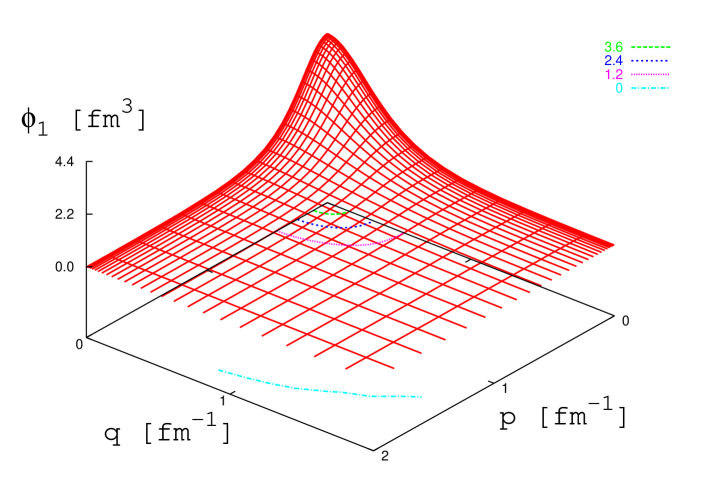
Figure 1: The dependence of the function $\phi_{1}(p,q,x=1)$ on $p$ and $q$. For better visibility also contour lines are given.

These functions $\phi_{i}({\bf p},{\bf q})$ depend on three variables, $p$, $q$, and ${\bf{\hat{p}}}\cdot{\bf{\hat{q}}}$. They are determined by the partial wave components of the 3N bound state and analytically known coefficient functions. In Figs. 1 through 4 we display $\phi_{1}(p,q,\cos\theta)$, $\phi_{8}(p,q,\cos\theta)$, $\phi_{7}(p,q,\cos\theta)$,and $\phi_{2}(p,q,\cos\theta)$ for a fixed angle $\theta=0$. We see that the numerically largest function is $\phi_{1}(p,q,\cos\theta)$, the other three ones shown are at least an order of magnitude smaller. While $\phi_{1}(p,q,\cos\theta)$ has a simple, bell-like shape with the maximum at $p=0$ and $q=0$, for $\phi_{8}(p,q,\cos\theta)$ the maximum is shifted to $p\approx 0.2$ and $q\approx 0.4$ fm^-1. The reason for this is that $\phi_{8}(p,q,\cos\theta)$ does not contain s-wave contributions but instead includes tensor force couplings. The function $\phi_{7}(p,q,\cos\theta)$ is similar in shape to $\phi_{8}(p,q,\cos\theta)$. Finally, $\phi_{2}(p,q,\cos\theta)$ also has its minimum shifted away from the origin.

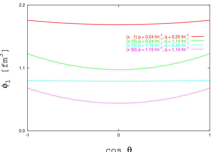
Figure 5: The angle dependence of $\phi_{1}(p,q,\cos\theta)$ for different pairs of momenta $p$ and $p$ as indicated in the figure. Note the multiplicative factors in three cases.

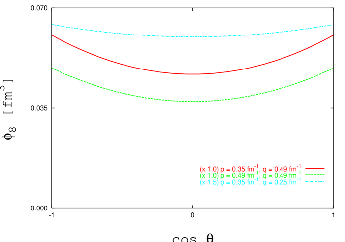
Figure 6: The angle dependence of $\phi_{8}(p,q,\cos\theta)$ for different pairs of momenta $p$ and $p$ as indicated in the figure. Note the multiplicative factors in two cases.

The dependence on the angle ${\bf{\hat{p}}}\cdot{\bf{\hat{q}}}$ is generally rather weak. In order to show the angular dependence explicitly, the function $\phi_{1}(p,q,\cos\theta)$ is displayed in Fig. 5 for some fixed values of $p$ and $q$ as function of $\cos\theta$. Similarly, we show in Fig. 6 the angular dependence of $\phi_{8}(p,q,\cos\theta)$. The angular dependence of $\phi_{7}(p,q,\cos\theta)$ and $\phi_{2}(p,q,\cos\theta)$ is dominantly given by $P_{1}(\cos\theta)$, and thus not displayed.

For the calculations presented in the following, we used a wave function based on the NN force AV18 R. B. Wiringa et al. (1995) in conjunction with the Urbana-IX three-nucleon force B. S. Pudliner et al. (1997). We show results for the ³He. The $\phi_{i}$ functions for other interactions are qualitatively similar, especially, their relative importance is not changed. Tabulated functions for several force combinations are provided by the authors url .

In order to quantify the relative importance of the eight functions $\phi_{i}({\bf p},{\bf q})$ we consider the normalization of the 3N bound state

$$\langle\Psi^{m=\frac{1}{2}}|\Psi^{m=\frac{1}{2}}\rangle=\sum_{i}\int d{\bf p}\;d{\bf q}\;\langle\chi_{i}|\chi_{i}\rangle\phi_{i}^{2}+2Re\sum_{i<j}\int d{\bf p}\;d{\bf q}\;\langle\chi_{i}|\chi_{j}\rangle\phi_{i}\phi_{j}$$ (39)

using the representation given in Eq. (36). The numerical evaluation is straightforward, and the contributions of the different products of the $\phi_{i}({\bf p},{\bf q})$ (denoted as $N_{ij}$) to the norm are listed in Table I. Clearly, the major contribution to the norm (91.42 %) is given by $\phi_{1}^{2}({\bf p},{\bf q})$. The second largest contribution is already more than one order of magnitude smaller and is given by $\phi_{8}^{2}({\bf p},{\bf q})$. All other contributions are even smaller.

IV Application

As example for the application of the above derived operator form of the 3N bound state we consider the spin dependent momentum distribution of a neutron inside a polarized ³He nucleus. This quantity is defined as

$$N({\bf q})=\langle\Psi^{m=\frac{1}{2}}|\delta({\bf q}-{\bf q}_{op})\frac{1}{2}(1+\sigma_{0}(3))|\Psi^{m=\frac{1}{2}}\rangle$$ (40)

It should be noted that in the 3N c.m. system the Jacobi momentum ${\bf q}$ is the momentum of one nucleon, here nucleon 3. Regarding the eight operator structures displayed in Eq. (37) one recognizes that only the following five different terms occur

$$O_{1} \equiv 1$$

$$O_{2} \equiv {\mbox{\boldmath$\sigma$}}(12)\cdot{\mbox{\boldmath$\sigma$}}(3)$$

$$O_{3} \equiv {\mbox{\boldmath$\sigma$}}(3)\cdot{\bf A}\equiv O_{3}({\bf A})$$

$$O_{4} \equiv {\mbox{\boldmath$\sigma$}}(12)\cdot{\bf B}\equiv O_{4}({\bf B})$$

$$O_{5} \equiv {\mbox{\boldmath$\sigma$}}(12)\cdot{\bf C}\;{\mbox{\boldmath$\sigma$}}(3)\cdot{\bf D}\equiv O_{5}({\bf C},{\bf D}).$$ (41)

Here the vectors A, B, C, and D represent different momentum vectors. It is a straightforward exercise to evaluate once and for all the matrix elements

$$\langle O_{i}^{\prime}O_{j}\rangle\equiv\langle\chi^{m}|O_{i}^{\prime}O_{j}|\chi^{m}\rangle.$$ (42)

The nonvanishing ones are listed below:

$$\langle O_{1}O_{1}\rangle = 1$$

$$\langle O_{1}O_{3}\rangle = A_{0}$$

$$\langle O_{2}O_{2}\rangle = 3$$

$$\langle O_{2}O_{4}\rangle = B_{0}$$

$$\langle O_{2}O_{5}\rangle = {\bf C}\cdot{\bf D}+i({\bf C}\times{\bf D})_{0}$$

$$\langle O_{3}^{\prime}O_{1}\rangle = A_{0}^{\prime}$$

$$\langle O_{3}^{\prime}O_{3}\rangle = {\bf A}^{\prime}\cdot{\bf A}+i({\bf A}^{\prime}\times{\bf A})_{0}$$

$$\langle O_{4}^{\prime}O_{2}\rangle = B_{0}^{\prime}$$

$$\langle O_{4}^{\prime}O_{4}\rangle = {\bf B}^{\prime}\cdot{\bf B}$$

$$\langle O_{4}^{\prime}O_{5}\rangle = ({\bf B}^{\prime}\cdot{\bf C})D_{0}$$

$$\langle O_{5}^{\prime}O_{2}\rangle = {\bf C}^{\prime}\cdot{\bf D}^{\prime}-i({\bf C}^{\prime}\times{\bf D}^{\prime})_{0}$$

$$\langle O_{5}^{\prime}O_{4}\rangle = ({\bf B}\cdot{\bf C}^{\prime})D_{0}^{\prime}$$

$$\langle O_{5}^{\prime}O_{5}\rangle = ({\bf C}^{\prime}\cdot{\bf C})[{\bf D}^{\prime}\cdot{\bf D}+i({\bf D}^{\prime}\times{\bf D})_{0}].$$ (43)

For the evaluation of the specific expectation value $N({\bf q})$ considered in Eq. (40) we need in addition matrix elements of the form

$$\langle O_{i}^{\prime}\sigma_{0}(3)O_{j}\rangle\equiv\langle\chi^{m}|O_{i}^{\prime}\sigma_{0}(3)O_{j}|\chi^{m}\rangle.$$ (44)

The resulting, nonvanishing matrix elements are listed in Appendix E. With this, the specific operator $\hat{O}$ for evaluating $N({\bf q})$ from Eq. (40) has spin matrix elements given as

$$\langle O_{i}^{\prime}\hat{O}O_{j}\rangle\equiv\langle O_{i}^{\prime}\frac{1}{2}(1+\sigma_{0}(3))O_{j}\rangle,$$ (45)

and the nonvanishing matrix elements are also listed in Appendix E. Next one expresses the states $|\chi_{i}\rangle$ in terms of the 5 operators $O_{i}$,

$$|\chi_{i}\rangle=\sum_{j}A_{ij}O_{j}(\Omega_{ij})|\chi^{m}\rangle,$$ (46)

where $\Omega_{ij}$ denotes the arguments of the operators $O_{j}$ which varies with $|\chi_{i}\rangle$. One explicitly obtains

$$|\chi_{1}\rangle = O_{1}|\chi^{m}\rangle$$

$$|\chi_{2}\rangle = \frac{1}{\sqrt{3}}O_{2}\mid\chi^{m}\rangle$$

$$|\chi_{3}\rangle = \sqrt{\frac{3}{2}}\frac{1}{i}\frac{O_{3}({\bf p}\times{\bf q})}{pq}\mid\chi^{m}\rangle$$

$$|\chi_{4}\rangle = \frac{1}{\sqrt{2}}\frac{1}{pq}\left(iO_{4}({\bf p}\times{\bf q})-O_{5}({\bf q},{\bf p})+O_{5}({\bf p},{\bf q})\right)\mid\chi^{m}\rangle$$

$$|\chi_{5}\rangle = \frac{1}{i}\left(\frac{O_{4}({\bf p}\times{\bf q})}{pq}-\frac{i}{2}\frac{O_{5}({\bf q},{\bf p})-O_{5}({\bf p},{\bf q})}{pq}\right)\mid\chi^{m}\rangle$$

$$|\chi_{6}\rangle = \sqrt{\frac{3}{2}}\left[\frac{O_{5}({\bf p},{\bf p})}{p^{2}}-\frac{1}{3}O_{2}\right]\mid\chi^{m}\rangle$$

$$|\chi_{7}\rangle = \sqrt{\frac{3}{2}}\left[\frac{O_{5}({\bf q},{\bf q})}{q^{2}}-\frac{1}{3}O_{2}\right]\mid\chi^{m}\rangle$$

$$|\chi_{8}\rangle = \frac{3}{2}\frac{1}{\sqrt{5}}\frac{1}{pq}\left[O_{5}({\bf q},{\bf p})+O_{5}({\bf p},{\bf q})-\frac{2}{3}{\bf p}\cdot{\bf q}O_{2}\right]\mid\chi^{m}\rangle.$$ (47)

Using the expectation values listed in Appendix E, one can determine the matrix elements $\langle\chi_{i}|\hat{O}|\chi_{j}\rangle$ in a straightforward fashion. As example we give

$$\langle\chi_{4}|\hat{O}|\chi_{6}\rangle=\frac{\sqrt{3}}{2}\frac{1}{pq}(\frac{i}{3}({\bf p}\times{\bf q})_{0}-\frac{p_{0}^{2}}{p^{2}}{\bf p}\cdot{\bf q}+p_{0}q_{0}).$$ (48)

Here the index 0 denotes a spherical component. The above expression nicely exhibits the analytic angular dependence. The final step in obtaining the momentum distribution $N({\bf q})$ is then to write

$$N({\bf q}) = \int d{\bf p}\;\langle\Psi^{m=\frac{1}{2}}(\hat{{\bf p}}\hat{{\bf q}})|\hat{O}|\Psi^{m=\frac{1}{2}}(\hat{{\bf p}}\hat{{\bf q}})\rangle$$ (49)

$$= \int d{\bf p}\;\Bigl{(}\sum_{i}\phi_{i}^{2}\langle\chi_{i}|\hat{O}|\chi_{i}\rangle+2\sum_{i<j}\phi_{i}\phi_{j}Re\langle\chi_{i}|\hat{O}|\chi_{j}\rangle\Bigr{)}.$$

An inspection of all analytically given spin matrix elements reveals that only four types of angular integrations occur. These are

$$\int d\hat{{\bf p}}\;f(\hat{{\bf p}}\cdot\hat{{\bf q}})\left\{\begin{array}[]{l}1\\ p_{0}\\ p_{0}^{2}\\ ({\bf p}\times{\bf q})_{0}^{2}\end{array}\right.$$ . (54)

Because of the rotational invariance around the quantization axis (z-axis) one can choose the vector ${\bf q}$ to be in the x-z plane. Then it is most convenient to rotate the z-axis into the direction of ${\bf q}$ by the angle $\theta\equiv\theta_{q}$. The result is

$$\int d\hat{{\bf p}}\;f(\hat{{\bf p}}\cdot\hat{{\bf q}})\left\{\begin{array}[]{l}1\\ p_{0}\\ p_{0}^{2}\\ ({\bf p}\times{\bf q})_{0}^{2}\end{array}\right. = 2\pi\int_{-1}^{1}dxf(x)\left\{\begin{array}[]{l}1\\ p\cos{\theta}x\\ p^{2}\left(\cos^{2}{\theta}x^{2}+\frac{1}{2}\sin^{2}{\theta}(1-x^{2})\right)\\ \frac{1}{2}p^{2}(1-x^{2})\end{array}\right..$$ (63)

Collecting all the results one ends with the final expression for $N({\bf q})\equiv N(q,\theta)$ given by

$$N(q,\theta) = 2\pi\int_{0}^{\infty}dp\;p^{2}\int_{-1}^{1}dx$$ (64)

$$\times\Bigl{\{}\phi_{1}^{2}(p,q,x)+\frac{1}{3}\phi_{2}^{2}(p,q,x)$$

$$+\phi_{2}(p,q,x)\phi_{6}(p,q,x)\frac{1}{3\sqrt{2}}(3\cos^{2}{\theta}-1)(3x^{2}-1)$$

$$+\phi_{2}(p,q,x)\phi_{7}(p,q,x)\frac{\sqrt{2}}{3}(3\cos^{2}{\theta}-1)$$

$$+\phi_{2}(p,q,x)\phi_{8}(p,q,x)\frac{2}{\sqrt{15}}(3\cos^{2}{\theta}-1)x$$

$$+\phi_{3}^{2}(p,q,x)\frac{3}{4}(1-\cos^{2}{\theta})(1-x^{2})$$

$$+\phi_{4}^{2}(p,q,x)\frac{1}{4}(3+\cos^{2}{\theta})(1-x^{2})$$

$$+\phi_{4}(p,q,x)\phi_{5}(p,q,x)\frac{1}{2\sqrt{2}}(\cos^{2}{\theta}-3)(1-x^{2})$$

$$+\phi_{4}(p,q,x)\phi_{6}(p,q,x)\frac{\sqrt{3}}{2}(3\cos^{2}{\theta}-1)(1-x^{2})x$$

$$+\phi_{4}(p,q,x)\phi_{8}(p,q,x)\frac{3}{2\sqrt{10}}(3\cos^{2}{\theta}-1)(1-x^{2})$$

$$+\phi_{5}^{2}(p,q,x)\frac{1}{8}(\cos^{2}{\theta}+9)(1-x^{2})$$

$$+\phi_{5}(p,q,x)\phi_{6}(p,q,x)\frac{1}{2}\sqrt{\frac{3}{2}}(3\cos^{2}{\theta}-1)(1-x^{2})x$$

$$+\phi_{5}(p,q,x)\phi_{8}(p,q,x)\frac{3}{4\sqrt{5}}(3\cos^{2}{\theta}-1)(1-x^{2})$$

$$+\phi_{6}^{2}(p,q,x)\frac{1}{12}[4+(3\cos^{2}{\theta}-1)(3x^{2}-1)]$$

$$+\phi_{6}(p,q,x)\phi_{7}(p,q,x)\frac{1}{6}(3\cos^{2}{\theta}+1)(3x^{2}-1)$$

$$+\phi_{6}(p,q,x)\phi_{8}(p,q,x)\frac{1}{2\sqrt{30}}[8+(3\cos^{2}{\theta}-1)(3x^{2}+1)]x$$

$$+\phi_{7}^{2}(p,q,x)\frac{1}{6}(3\cos^{2}{\theta}+1)$$

$$+\phi_{7}(p,q,x)\phi_{8}(p,q,x)\sqrt{\frac{2}{15}}(3\cos^{2}{\theta}+1)x$$

$$+\phi_{8}^{2}(p,q,x)\frac{1}{200}[48+(15\cos^{2}{\theta}-1)(5x^{2}+3)]\Bigr{\}}.$$

Though the angular dependence for the direction of the nucleon momentum ${\bf q}$ in relation to the quantization axis is analytically given, the full expression is quite lengthy. However the dependence on the angle $\theta$ is quite simple, namely $N(q,\theta)\equiv a(q)+b(q)\cos^{2}\theta$. Moreover most of the contributions are numerically insignificant, as illustrated in the previous section. Therefore, we only keep $\phi_{1}$, $\phi_{8}$, $\phi_{7}$, $\phi_{2}$. It turns out that for the specific quantity $N(q,\theta)$ only these components visibly contribute. Therefore, in this case the lengthy expression of Eq. (64) shrinks to the few leading terms

$$N(q,\theta) = 2\pi\int_{0}^{\infty}dp\;p^{2}\int_{-1}^{1}dx$$ (65)

$$\times\Bigl{\{}\phi_{1}^{2}(p,q,x)+\frac{1}{3}\phi_{2}^{2}(p,q,x).$$

$$+\phi_{2}(p,q,x)\phi_{7}(p,q,x)\frac{\sqrt{2}}{3}(3\cos^{2}{\theta}-1)$$

$$+\phi_{2}(p,q,x)\phi_{8}(p,q,x)\frac{2}{\sqrt{15}}(3\cos^{2}{\theta}-1)x$$

$$+\phi_{7}^{2}(p,q,x)\frac{1}{6}(3\cos^{2}{\theta}+1)$$

$$+\phi_{7}(p,q,x)\phi_{8}(p,q,x)\sqrt{\frac{2}{15}}(3\cos^{2}{\theta}+1)x$$

$$+\phi_{8}^{2}(p,q,x)\frac{1}{200}[48+(15\cos^{2}{\theta}-1)(5x^{2}+3)]\Bigr{\}}$$

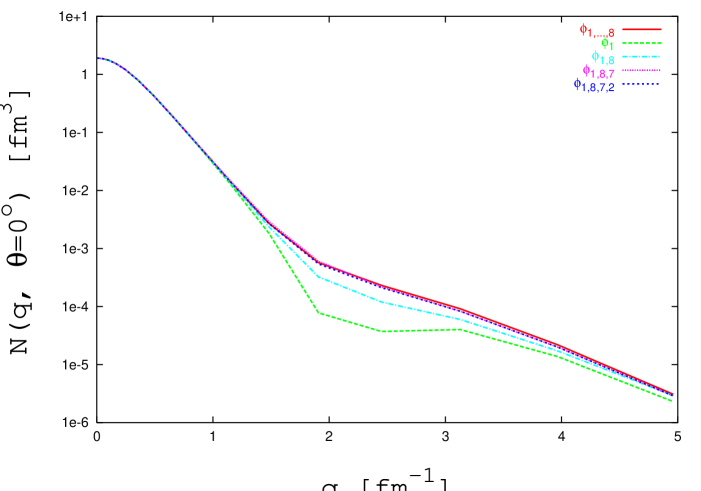
Figure 7: The momentum distribution $N(q,\theta=0)$. The solid line represents the calculation containing all terms in Eq. (64). The dashed line displays the result based on the first term only, the dash-dotted the one containing in addition the contribution of $\phi_{8}$. For the dotted line contributions containing $\phi_{7}$ are added. The long dashed-line contains in addition contributions including $\phi_{2}$ and corresponds to Eq. (65).

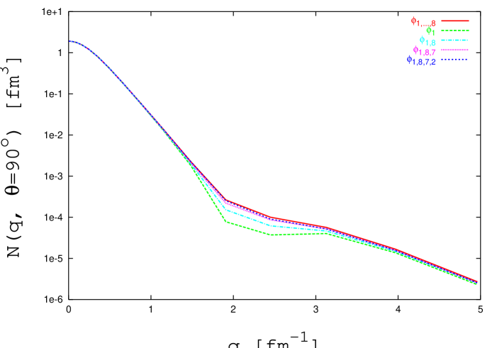
Figure 8: Same as Fig. 7, but for $N(q,\theta=90)$.

The numerical results for $N({\bf q})$ are displayed as function of $q$ in Fig. 7 for the fixed angle $\theta=0$ (i.e. the nucleon momentum is parallel to the quantization axis) and in Fig. 8 for $\theta=90^{o}$. We compare the full result given in Eq. (64) to various truncated sums. The solid line in Figs. 7 and 8 corresponds to the full calculation using Eq. (64). The most simple approximation would be to consider only the first term in Eq. (64) or Eq. (65), namely $\phi_{1}^{2}$, given by the dashed line. We see that this simple term alone already gives a good representation of $N(q,\theta)$ up to about $q\approx 1$ fm^-1. The dip around 2 fm^-1 is mostly filled in by adding the term containing $\phi_{8}^{2}$, shown as dash-dotted line. When adding terms containing $\phi_{7}$, represented by the dotted line, one is very close to the full result. Adding the terms containing $\phi_{2}$, i.e. calculating the expression given in Eq. (65), shows that all other terms in Eq. (64) are insignificant.

We expect that also for other observables the operator form of the 3N bound state will be useful. It should provide an easy access to the wave function without the need of having access to a modern triton code.

V Summary

An old idea by Gerjuoy and Schwinger Gerjuoy and Schwinger (1942) has been revived to present the 3N bound state in operator form. This form analytically exhibits the dominant angular and spin dependence of the wave function in form of scalar operators formed out of momentum and spin vectors, which are applied on a pure spin 1/2 state. Each such operator is accompanied by a scalar function depending on the magnitudes of the two Jacobi momenta and the angle between them. We established the connection of this form with the standard partial wave decomposition. This connection provided the explicit form of the scalar functions in terms of partial wave function components. The key point in the derivation was, to extract from an infinite sum of partial wave expressions the operator form and the accompanying scalar functions. The presented operator form of the 3N wave function is independent of the applied NN and 3N force.

We illustrated the application of this new form of the 3N bound state wave function by calculating the spin dependent single nucleon momentum distribution in a polarized 3N bound state. It turned out that for this quantity only 4 parts out of the total number of 8 parts forming the 3N bound state were needed to achieve a sufficiently accurate representation. Several sets of spin matrix elements depending on the Jacobi momentum vectors, which have to be calculated only once, have been evaluated. They will also be needed in other applications.

We expect that this operator form allows an easy access to the 3N bound state. The 8 scalar functions carrying the specific dynamical information have been tabulated on a sufficiently fine grid and can be downloaded from url . There are sets of scalar functions for various modern NN and 3N force combinations.

Appendix A Relation for the coupled spherical harmonics

Here the relation of Eq. (11) for the coupled spherical harmonics ${\mathcal{Y}}^{1\mu}_{ll}({\hat{\bf p}}{\hat{\bf q}})$ will be verified. We consider ${\mathcal{Y}}^{00}_{ll}({\hat{\bf p}}{\hat{\bf q}}){\mathcal{Y}}^{1\mu}_{11}({\hat{\bf p}}{\hat{\bf q}})$, which can be rewritten by standard techniques (see e.g. Glöckle (1983)) as

$${\mathcal{Y}}^{00}_{ll}({\hat{\bf p}}{\hat{\bf q}}){\mathcal{Y}}^{1\mu}_{11}({\hat{\bf p}}{\hat{\bf q}})=\frac{3}{4\pi}\sqrt{2l+1}\sum_{ab}(-)^{a+l}C(l1a,00)\>C(l1b,00)\left\{\begin{array}[]{ccc}b\>a\>1\\ 1\>1\>l\end{array}\right\}{\mathcal{Y}}^{1\mu}_{ab}({\hat{\bf p}}{\hat{\bf q}}).$$ (66)

The sum over $a$ and $b$ will give four terms. After inserting the explicit expression for the Clebsch-Gordon coefficients and the 6-j symbol, one arrives at

$${\mathcal{Y}}^{00}_{ll}({\hat{\bf p}}{\hat{\bf q}}){\mathcal{Y}}^{1\mu}_{11}({\hat{\bf p}}{\hat{\bf q}})=-\frac{3}{4\pi}\frac{1}{\sqrt{2l+1}}\frac{1}{\sqrt{6}}\left(-\sqrt{\frac{(l+1)(l+2)}{2l+3}}{\mathcal{Y}}^{1\mu}_{l+1\,l+1}+\sqrt{\frac{l(l+1)}{2l-1}}{\mathcal{Y}}^{1\mu}_{l-1\,l-1}\right).$$ (67)

Using the relation

$${\mathcal{Y}}^{00}_{ll}({\hat{\bf p}}{\hat{\bf q}})=(-)^{l}\frac{\sqrt{2l+1}}{4\pi}P_{l}({\hat{\bf p}}\cdot{\hat{\bf q}})$$ (68)

the previous Eq. (67) can be rewritten as

$${\mathcal{Y}}^{1\mu}_{ll}({\hat{\bf p}}{\hat{\bf q}}) = \sqrt{\frac{2l+1}{l(l+1)}}$$ (69)

$$\times\left((-)^{l+1}\sqrt{\frac{2}{3}}(2l-1)P_{l-1}({\hat{\bf p}}\cdot{\hat{\bf q}}){\mathcal{Y}}^{1\mu}_{11}({\hat{\bf p}}{\hat{\bf q}})+\sqrt{\frac{(l-1)(l-2)}{2l-3}}{\mathcal{Y}}^{1\mu}_{l-2\,l-2}({\hat{\bf p}}{\hat{\bf q}})\right).$$

This is a recursive formula and leads to the relation given in Eq. (11). In practice only low orbital angular momenta occur and one easily works out the lowest terms as

$$c_{1}({\hat{\bf p}}{\hat{\bf q}}) = 1$$

$$c_{2}({\hat{\bf p}}{\hat{\bf q}}) = -\sqrt{5}P_{1}({\hat{\bf p}}\cdot{\hat{\bf q}})$$

$$c_{3}({\hat{\bf p}}{\hat{\bf q}}) = \frac{1}{3}\sqrt{\frac{7}{2}}\left(5P_{2}({\hat{\bf p}}\cdot{\hat{\bf q}})+1\right).$$ (70)

Appendix B Verification of the relation given in Eq. (18)

The first step is to generate the spin states of Eq. (17) from the states $\mid\chi^{m}\rangle$ given in Eq. (5). It is easy to see that

$$\mid(1\frac{1}{2})\frac{3}{2}\frac{3}{2}\rangle=\sigma(12)_{+}\mid\chi^{m=\frac{1}{2}}\rangle,$$ (71)

where $\sigma_{+}(12)$ is the spherical component of the spin operator given in Eq. (6).

This form can be rewritten as

$$\mid(1\frac{1}{2})\frac{3}{2}\frac{3}{2}\rangle = \Big{(}\frac{2}{3}\sigma_{+}(12)+\frac{1}{3}\sigma_{(+)}(12)\Big{)}\mid\chi^{m=\frac{1}{2}}\rangle$$ (72)

$$= \frac{2}{3}\Big{(}\sigma_{+}(12)-\frac{i}{2}\Big{(}{\vec{\sigma}}(3)\times{\vec{\sigma}}(12)\Big{)}_{+}\Big{)}\mid\chi^{m=\frac{1}{2}}\rangle$$

using the spherical component of the vector product.

Next, we express the second spin state in Eq. (17) with the help of the lowering operator as

$$\mid(1\frac{1}{2})\frac{3}{2}\frac{1}{2}\rangle = ({\mathcal{S}}_{x}-i{\mathcal{S}}_{y})\mid(1\frac{1}{2})\frac{3}{2}\frac{3}{2}\rangle{1\over\sqrt{3}}$$ (73)

$$= {1\over\sqrt{6}}\Big{(}\sigma_{-}(1)+\sigma_{-}(2)+\sigma_{-}(3)\Big{)}\frac{1}{2}\Big{(}\sigma_{+}(1)-\sigma_{+}(2)\Big{)}\mid\chi^{m=\frac{1}{2}}\rangle$$

$$= {1\over\sqrt{6}}\frac{1}{2}\Big{(}2(\sigma_{0}(1)-\sigma_{0}(2)+\sigma_{-}(3)\Big{(}\sigma_{+}(1)-\sigma_{+}(2)\Big{)}\Big{)}\mid\chi^{m=\frac{1}{2}}\rangle$$

$$= {1\over\sqrt{6}}\frac{1}{2}\Big{(}2(\sigma_{0}(1)-\sigma_{0}(2))+i\Big{(}({\vec{\sigma}}(1)-{\vec{\sigma}}(2))\times{\vec{\sigma}}(3)\Big{)}_{0}\Big{)}\mid\chi^{m=\frac{1}{2}}\rangle$$

$$= {2\over\sqrt{6}}\Big{(}\sigma_{0}(12)-\frac{i}{2}({\vec{\sigma}}(3)\times{\vec{\sigma}}(12))_{0}\Big{)}\mid\chi^{m=\frac{1}{2}}\rangle.$$

Finally, starting from

$$\mid(1\frac{1}{2})\frac{3}{2}-\frac{1}{2}\;\rangle\;=\;\frac{1}{2}({\mathcal{S}}_{x}-i{\mathcal{S}}_{y})\mid(1\frac{1}{2})\frac{3}{2}\frac{1}{2}\;\rangle$$ (74)

inserting the form (B.3) and reshuffling leads to

$$\mid(1\frac{1}{2})\frac{3}{2}-\frac{1}{2}\;\rangle\;=\;\frac{2}{\sqrt{3}}\Big{(}{\vec{\sigma}}(12)_{-}-\frac{i}{2}({\vec{\sigma}}(3)\times{\vec{\sigma}}(12))_{-}\;\Big{)}\;\mid\chi^{m=\frac{1}{2}}\rangle$$ (75)

Now we use the relation (2.10) and the property

$${\mathcal{Y}}^{1\mu}_{11}({\hat{\bf p}}{\hat{\bf q}})=i\frac{3}{4\pi}\frac{1}{\sqrt{2}}{({\vec{p}}\times{\vec{q}})_{\mu}\over\mid{\vec{p}}\mid\mid{\vec{q}}\mid}.$$ (76)

With this one arrives directly at Eq. (18).

Appendix C Verification of the relation given in Eq. (21)

With standard recoupling techniques one finds

$${\mathcal{Y}}^{00}_{ll}({\hat{\bf p}}{\hat{\bf q}}){\mathcal{Y}}^{2m}_{11}({\hat{\bf p}}{\hat{\bf q}}) = {3\over 4\pi}{1\over 2l+1}\Bigg{(}\sqrt{{(l+1)(l+2)(2l+5)\over 30(2l+3)}}\>{\mathcal{Y}}^{2m}_{l+1l+1}$$ (77)

$$-\sqrt{{l(l+1)\over 5}}({\mathcal{Y}}^{2m}_{l+1,l-1}+{\mathcal{Y}}^{2-}_{l-1l+1})+\sqrt{{l(l-1)(2l-3)\over(2l-1)\cdot 30}}\>{\mathcal{Y}}^{2m}_{l-1,l-1}\Bigg{)},$$

which leads to the recursive relation

$${\mathcal{Y}}^{2m}_{ll} = \sqrt{{30(2l+1)\over l(l+1)(2l+3)}}\>\Bigg{\{}{4\pi\over 3}(2l-1){\mathcal{Y}}^{00}_{l-1l-1}{\mathcal{Y}}^{2m}_{11}$$ (78)

$$+\sqrt{{(l-1)l\over 5}}\>({\mathcal{Y}}^{2m}_{ll-2}+{\mathcal{Y}}^{2m}_{l-2l})-\sqrt{{(l-1)(l-2)(2l-5)\over(2l-3)30}}\>{\mathcal{Y}}^{2m}_{l-2l-2}\Bigg{\}}.$$

Similarly, starting from

$${\mathcal{Y}}^{00}_{ll}({\hat{\bf p}}{\hat{\bf q}})Y_{2m}({\hat{\bf p}}) = {1\over\sqrt{4\pi}}\Bigg{(}\sqrt{3\over 2}\>\sqrt{{(l+1)(l+2)\over(2l+1)(2l+3)}}\>{\mathcal{Y}}^{2m}_{l+2l}$$ (79)

$$-\sqrt{{l(l+1)\over(2l-1)(2l+3)}}\>{\mathcal{Y}}^{2m}_{ll}+\sqrt{3\over 2}\>\sqrt{{l(l-1)\over(2l-1)(2l+1)}}\>{\mathcal{Y}}^{2m}_{l-2l}\Bigg{)},$$

one finds the additional recursive relations

$${\mathcal{Y}}^{2m}_{l+2l}(\hat{{\bf p}}\hat{{\bf q}}) = \sqrt{2\over 3}\>\sqrt{{(2l+1)(2l+3)\over(l+1)(l+2)}}\>\Bigg{\{}\sqrt{4\pi}\>{\mathcal{Y}}^{00}_{ll}Y_{2m}({\hat{\bf p}})$$ (80)

$$+\sqrt{{l(l+1)\over(2l-1)(2l+3)}}\>{\mathcal{Y}}^{2m}_{ll}-\sqrt{3\over 2}\>\sqrt{{l(l-1)\over(2l-1)(2l+1)}}\>{\mathcal{Y}}^{2m}_{l-2,l}\Bigg{\}}$$

and similarly

$${\mathcal{Y}}^{2m}_{l,l+2}(\hat{{\bf p}}\hat{{\bf q}}) = \sqrt{2\over 3}\>\sqrt{{(2l+1)(2l+3)\over(l+1)(l+2)}}\>\Bigg{\{}\sqrt{4\pi}\>{\mathcal{Y}}^{00}_{ll}Y_{2m}({\hat{\bf q}})$$ (81)

$$+\sqrt{{l(l+1)\over(2l-1)(2l+3)}}\>{\mathcal{Y}}^{2m}_{ll}-\sqrt{3\over 2}\>\sqrt{{l(l-1)\over(2l-1)(2l+1)}}\>{\mathcal{Y}}^{2m}_{l,l-2}\Bigg{\}}.$$

Inserting these equations into each other yields the relations given in Eqs. (21). For the calculation of a 3N bound state, the scalar functions $A_{l}$ to $E_{l}$ are in practice only needed for small values of $l$. In our context we only need odd values of $l$. The two lowest cases are given here.

If only $l=1$ is kept, then one trivially has $A_{1}=1$ and $B_{1}=0$, and all other terms are absent. If only $l=1$ and $l=3$ are kept, then one obtains from Eqs. (C.4) and (C.5)

$${\mathcal{Y}}^{2m}_{31}({\hat{\bf p}}{\hat{\bf q}}) = \sqrt{2\over 3}\>{\mathcal{Y}}^{2m}_{11}-\sqrt{5\over 4\pi}P_{1}Y_{2m}({\hat{\bf p}})$$

$${\mathcal{Y}}^{2m}_{13}({\hat{\bf p}}{\hat{\bf q}}) = \sqrt{2\over 3}\>{\mathcal{Y}}^{2m}_{11}-\sqrt{5\over 4\pi}P_{1}Y_{2m}({\hat{\bf q}}).$$ (82)

Furthermore, Eq. (C.2) yields

$${\mathcal{Y}}^{2m}_{33}({\hat{\bf p}}{\hat{\bf q}})=\sqrt{35\over 18}\Bigg{\{}{\mathcal{Y}}^{2m}_{11}({\hat{\bf p}}{\hat{\bf q}})({5\sqrt{5}\over 3}P_{2}-\sqrt{1\over 45})+\sqrt{6\over 5}({\mathcal{Y}}^{2m}_{13}+{\mathcal{Y}}^{2m}_{31})\Bigg{\}}$$ (83)

and after insertion of the results (C.6) we get

$${\mathcal{Y}}^{2m}_{33}({\hat{\bf p}}{\hat{\bf q}})={\mathcal{Y}}^{2m}_{11}\sqrt{7\over 2}{1\over 9}(25P_{2}({\hat{\bf p}}{\hat{\bf q}})+11)-\sqrt{35\over 12\pi}P_{1}({\hat{\bf p}}{\hat{\bf q}})\Big{(}Y_{2m}({\hat{\bf p}})+Y_{2m}({\hat{\bf q}})\Big{)}.$$ (84)

Thus, one obtains in the end the coefficients given in Eq. (30).

Appendix D The Operators of Eq. (26)

The starting points for the derivation are Eqs. (19) and (22). According to Eqs. (72), (73), and (75) these lead to

$$\mid\,^{4}D^{m=\frac{1}{2}}_{\frac{1}{2}}\rangle = -{2\over 3}\sqrt{1\over 10}\Big{(}\sigma(12)-{i\over 2}(\sigma(3)\times\sigma(12))\Big{)}_{+}\mid\,\chi^{m=\frac{1}{2}}\rangle$$ (85)

$$\times\sum_{lodd}\Big{(}{\mathcal{Y}}^{2-1}_{11}({\hat{\bf p}}{\hat{\bf q}})X_{l}+Y_{2-1}({\hat{\bf p}})V_{l}+Y_{2-1}({\hat{\bf q}})W_{l}\Big{)}$$

$$+\sqrt{1\over 5}{2\over\sqrt{6}}\Big{(}\sigma(12)-{i\over 2}\sigma(3)\times\sigma(12)\Big{)}_{0}\mid\,\chi^{m=\frac{1}{2}}\rangle$$

$$\times\sum_{lodd}\Big{(}{\mathcal{Y}}^{20}_{11}({\hat{\bf p}}{\hat{\bf q}})X_{l}+Y_{20}({\hat{\bf p}})V_{l}+Y_{20}({\hat{\bf q}})W_{l}\Big{)}$$

$$-\sqrt{3\over 10}{2\over\sqrt{3}}\Big{(}\sigma(12)-{i\over 2}(\sigma(3)\times\sigma(12))_{-}\mid\chi^{m=\frac{1}{2}}\rangle$$

$$\times\sum_{lodd}\Big{(}{\mathcal{Y}}^{21}_{11}({\hat{\bf p}}{\hat{\bf q}})X_{l}+Y_{21}({\hat{\bf p}})V_{l}+Y_{21}({\hat{\bf q}})W_{l}\Big{)}$$

$$+\sqrt{2\over 5}\sqrt{1\over 2}\sigma_{-}(3)\sigma_{-}(12)\mid\chi^{m=\frac{1}{2}}\rangle\sum_{lodd}\Big{(}{\mathcal{Y}}^{22}_{11}({\hat{\bf p}}{\hat{\bf q}})X_{l}+Y_{22}({\hat{\bf p}})V_{l}+Y_{22}({\hat{\bf q}})W_{l}\Big{)}.$$

As an example let us regard the terms in $Y_{2\mu}({\hat{\bf p}})$, which have the well known representation in terms of spherical components of ${\bf p}$:

$$Y_{2-1}({\hat{\bf p}}) = {1\over 2{\bf p}^{2}}\sqrt{15\over\pi}p_{0}p_{-}$$

$$Y_{20}({\hat{\bf p}}) = {1\over 2{\bf p}^{2}}\sqrt{5\over\pi}\left(p_{0}^{2}+p_{+}p_{-}\right)$$

$$Y_{21}({\hat{\bf p}}) = {1\over 2{\bf p}^{2}}\sqrt{15\over\pi}p_{0}p_{+}$$

$$Y_{22}({\hat{\bf p}}) = {1\over 2{\bf p}^{2}}\sqrt{15\over 2\pi}(p_{+})^{2}.$$ (86)

For the convenience of the reader we also provide the relations

$${\mathcal{Y}}^{2-1}_{11}({\hat{\bf p}}{\hat{\bf q}}) = {1\over\sqrt{2}}{3\over 4\pi}{1\over\mid{\bf p}\mid\mid{\bf q}\mid}\left(p_{0}q_{-}+p_{-}q_{0}\right)$$

$${\mathcal{Y}}^{20}_{11}({\hat{\bf p}}{\hat{\bf q}}) = {3\over 4\pi}{1\over\mid{\bf p}\mid\mid{\bf q}\mid}\left({1\over\sqrt{6}}(p_{+}q_{-}+p_{-}q_{+})+\sqrt{{2\over 3}}p_{0}q_{0}\right)$$

$${\mathcal{Y}}^{21}_{11}({\hat{\bf p}}{\hat{\bf q}}) = {1\over\sqrt{2}}{3\over 4\pi}{1\over\mid{\bf p}\mid\mid{\bf q}\mid}\left(p_{+}q_{0}+p_{0}q_{+}\right)$$

$${\mathcal{Y}}^{22}_{11}({\hat{\bf p}}{\hat{\bf q}}) = {3\over 4\pi}{p_{+}q_{+}\over\mid{\bf p}\mid\mid{\bf q}\mid}.$$ (87)

If one now inserts (D.2) into (D.1) and looks only into the terms with $V_{l}$, one can easily combine the expressions to

$$\mid\,4D^{m}_{\frac{1}{2}}\rangle\Big{|}_{V_{l}}=\frac{1}{2}{\sqrt{3\over 2\pi}}\sum_{lodd}V_{l}\left[{{\bf\sigma}(12)\cdot{\bf p}\;{\bf\sigma}(3)\cdot{\bf p}\over{\bf p}^{2}}-\frac{1}{3}{\bf\sigma}(12)\cdot{\bf\sigma}(3)\right]\mid\chi^{m}\rangle$$ (88)

The term in $X_{l}$ is somewhat more tedious.

Appendix E The Nonvanishing Matrixelements of Eqs. (44) and (45)

The nonvanishing matrix elements of Eq. (44) are given by

$$\langle O_{1}\sigma_{0}(3)O_{1}\rangle = 1$$

$$\langle O_{1}\sigma_{0}(3)O_{3}\rangle = A_{0}$$

$$\langle O_{2}\sigma_{0}(3)O_{2}\rangle = -1$$

$$\langle O_{2}\sigma_{0}(3)O_{4}\rangle = B_{0}$$

$$\langle O_{2}\sigma_{0}(3)O_{5}\rangle = 2C_{0}D_{0}-{\bf C}\cdot{\bf D}-i({\bf C}\times{\bf D})_{0}$$

$$\langle O_{3}^{\prime}\sigma_{0}(3)O_{1}\rangle = A_{0}^{\prime}$$

$$\langle O_{3}^{\prime}\sigma_{0}(3)O_{3}\rangle = 2A_{0}^{\prime}A_{0}-{\bf A}^{\prime}\cdot{\bf A}-i({\bf A}^{\prime}\times{\bf A})_{0}$$

$$\langle O_{4}^{\prime}\sigma_{0}(3)O_{2}\rangle = B_{0}^{\prime}$$

$$\langle O_{4}^{\prime}\sigma_{0}(3)O_{4}\rangle = {\bf B}^{\prime}\cdot{\bf B}$$

$$\langle O_{4}^{\prime}\sigma_{0}(3)O_{5}\rangle = ({\bf B}^{\prime}\cdot{\bf C})D_{0}$$

$$\langle O_{5}^{\prime}\sigma_{0}(3)O_{2}\rangle = 2C_{0}^{\prime}D_{0}^{\prime}-{\bf C}^{\prime}\cdot{\bf D}^{\prime}+i({\bf C}^{\prime}\times{\bf D}^{\prime})_{0}$$

$$\langle O_{5}^{\prime}\sigma_{0}(3)O_{4}\rangle = ({\bf B}\cdot{\bf C}^{\prime})D_{0}^{\prime}$$

$$\langle O_{5}^{\prime}\sigma_{0}(3)O_{5}\rangle = ({\bf C}^{\prime}\cdot{\bf C})[2D_{0}^{\prime}D_{0}-{\bf D}^{\prime}\cdot{\bf D}-i({\bf D}^{\prime}\times{\bf D})_{0}].$$ (89)

The nonvanishing matrix elements of Eq. (45) are given by

$$\langle O_{1}\hat{O}O_{1}\rangle = 1$$

$$\langle O_{1}\hat{O}O_{3}\rangle = A_{0}$$

$$\langle O_{2}\hat{O}O_{2}\rangle = 1$$

$$\langle O_{2}\hat{O}O_{4}\rangle = B_{0}$$

$$\langle O_{2}\hat{O}O_{5}\rangle = C_{0}D_{0}$$

$$\langle O_{3}^{\prime}\hat{O}O_{1}\rangle = A_{0}^{\prime}$$

$$\langle O_{3}^{\prime}\hat{O}O_{3}\rangle = A_{0}^{\prime}A_{0}$$

$$\langle O_{4}^{\prime}\hat{O}O_{2}\rangle = B_{0}^{\prime}$$

$$\langle O_{4}^{\prime}\hat{O}O_{4}\rangle = {\bf B}^{\prime}\cdot{\bf B}$$

$$\langle O_{4}^{\prime}\hat{O}O_{5}\rangle = ({\bf B}^{\prime}\cdot{\bf C})D_{0}$$

$$\langle O_{5}^{\prime}\hat{O}O_{2}\rangle = C_{0}^{\prime}D_{0}^{\prime}$$

$$\langle O_{5}^{\prime}\hat{O}O_{4}\rangle = ({\bf B}\cdot{\bf C}^{\prime})D_{0}^{\prime}$$

$$\langle O_{5}^{\prime}\hat{O}O_{5}\rangle = ({\bf C}^{\prime}\cdot{\bf C})D_{0}^{\prime}D_{0}.$$ (90)

Table 1: The contributions $N_{ij}$ from $\phi_{i}({\bf p},{\bf q})\phi_{j}({\bf p},{\bf q})$ to the total normalization of the 3N state.

$ij$	$11$	$22$	$33$	$44$	$55$	$66$	$67$	$68$	$77$	$78$	$88$
$N_{ij}$ [%]	91.42	0.76	0.02	0.02	0.02	0.13	0.11	0.25	0.98	2.44	4.35

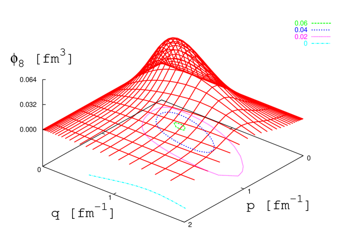
Figure 2: The dependence of the function $\phi_{8}(p,q,x=1)$ on $p$ and $q$. For better visibility also contour lines are given.

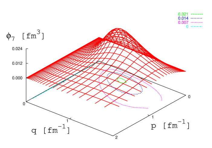
Figure 3: The dependence of the function $\phi_{7}(p,q,x=1)$ on $p$ and $q$. For better visibility also contour lines are given.

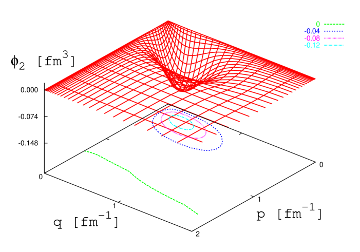
Figure 4: The dependence of the function $\phi_{2}(p,q,x=1)$ on $p$ and $q$. For better visibility also contour lines are given.

References

- Nogga et al. (2000) A. Nogga, H. Kamada, and W. Glöckle, Phys. Rev. Lett. 85, 944 (2000).
- Nogga et al. (2002) A. Nogga, H. Kamada, W. Glöckle, and B. R. Barrett, Phys. Rev. C 65, 054003 (2002).
- A. Kievsky et al. (1993) A. Kievsky, M. Viviani, and S. Rosati, Nucl. Phys. A551, 241 (1993).
- A. Kievsky (1997) A. Kievsky, Nucl. Phys. A624, 125 (1997).
- Kamimura (1988) M. Kamimura, Phys. Rev. A 38, 621 (1988).
- Pieper and Wiringa (2001) S. C. Pieper and R. B. Wiringa, Ann. Rev. Nucl. Part. Sci. 51, 53 (2001).
- P. Navrátil and B. R. Barrett (1998) P. Navrátil and B. R. Barrett, Phys. Rev. C 57, 562 (1998).
- Elster et al. (1999) C. Elster, W. Schadow, A. Nogga, and W. Glöckle, Few Body Syst. 27, 83 (1999).
- Liu et al. (2002) H. Liu, C. Elster, and W. Glöckle, Comput. Phys. Commun. 147, 170 (2002).
- Liu et al. (2003) H. Liu, C. Elster, and W. Glöckle, Few-Body Systems 33, 241 (2003).
- Rarita and Schwinger (1941a) W. Rarita and J. Schwinger, Phys. Rev. 59, 436 (1941a).
- Rarita and Schwinger (1941b) W. Rarita and J. Schwinger, Phys. Rev. 59, 556 (1941b).
- Fachruddin et al. (2001) I. Fachruddin, C. Elster, and W. Glöckle, Phys. Rev. C 63, 054003 (2001).
- Forest et al. (1996) J. L. Forest, V. R. Pandharipande, S. C. Pieper, R. B. Wiringa, R. Schiavilla, and A. Arriaga, Phys. Rev. C 54, 646 (1996).
- Gerjuoy and Schwinger (1942) E. Gerjuoy and J. Schwinger, Phys. Rev. 61, 138 (1942).
- Glöckle (1983) W. Glöckle, The Quantum Mechanical Few-Body Problem (Springer-Verlag, Berlin, 1983).
- Rose (1957) M. E. Rose, Elementary Theory of Angular Momentum (Wiley, New York, 1957).
- R. B. Wiringa et al. (1995) R. B. Wiringa, V. G. J. Stoks, and R. Schiavilla, Phys. Rev. C 51, 38 (1995).
- B. S. Pudliner et al. (1997) B. S. Pudliner, V. R. Pandharipande, J. Carlson, Steven C. Pieper, and R. B. Wiringa, Phys. Rev. C 56, 1720 (1997).
- (20) The scalar functions are available at http://www.phy.ohiou.edu/~elster/h3wave.