Weak non-mesonic decay of Hypernuclei

Abstract

We review the mechanism of weak decay of hypernuclei, with emphasis on the non-mesonic decay channels. Various theoretical approaches are discussed and the results are compared with the available experimental data.

PACS: 21.80.+a; 13.75.Ev; 25.40.-h

1 Introduction

The main decay modes of $\Lambda$-hypernuclei are the so-called mesonic and non-mesonic decays(for a recent review on the argument see ref. [1]): the former also occurs for free $\Lambda$-hyperons:

$$\Lambda\rightarrow\left\{\begin{array}[]{l l }\pi^{-}p&(\Gamma^{\rm free}_{\pi^{-}}/\Gamma^{\rm free}_{\Lambda}=0.639)\\ \pi^{0}n&(\Gamma^{\rm free}_{\pi^{0}}/\Gamma^{\rm free}_{\Lambda}=0.358),\end{array}\right.$$ (1)

The experimental ratio of the relevant widths, $\Gamma^{\rm free}_{\pi^{-}}/\Gamma^{\rm free}_{\pi^{0}}\simeq 1.78$, together with the measurements of $\Lambda$ polarization observables lead to the formulation of the $\Delta I=1/2$ rule on the isospin change of the system [from simple Clebsch-Gordon coefficient analysis, the latter would predict $\Gamma^{\rm free}_{\pi^{-}}/\Gamma^{\rm free}_{\pi^{0}}=2$]. This rule is based on experimental observations, but its dynamical origin is not yet understood on theoretical grounds. The Standard Model does not support it and many non-perturbative effects could be responsible for the measured enhancement of the $\Delta I=1/2$ transition amplitude.

The mesonic decay can also take place in $\Lambda$-hypernuclei, however the Pauli principle tends to disfavour the produced final state, with an emitted nucleon of momentum $p_{N}\simeq 100$ MeV/c (from a $\Lambda$ at rest), well below the maximum level of occupied states in the nucleus. Of course this argument is only a qualitative one: indeed the mesonic decay is an important fraction of the total decay rate in light-medium $\Lambda$-hypernuclei. This outcome stems from several facts: i) the hyperon momentum distribution in the nucleus, ii) the medium attraction on the emitted pion, which lowers its mass at fixed momentum and distorts the pionic outgoing wave, iii) the strong reduction of the local Fermi momentum at the nuclear surface.[2]

Notably the mesonic decay can be used to extract information on the pion–nucleus optical potential (in a complementary way with respect to pionic atoms and low energy $\pi$-nucleus scattering experiments).

The $\Lambda$-hypernuclei non-mesonic decay occurs via the weak interaction of the $\Lambda$ with one nucleon:

$$\Lambda N\to NN\qquad\qquad\mbox{ {(one-body induced decay)}}$$

or with a pair of correlated nucleons:

$$\Lambda NN\to NNN\qquad\qquad\mbox{ {(two-body induced decay)}}.$$

These processes are mediated by the exchange of a meson (including the $K$, $K^{*}$ strange mesons), as illustrated in Fig. 1

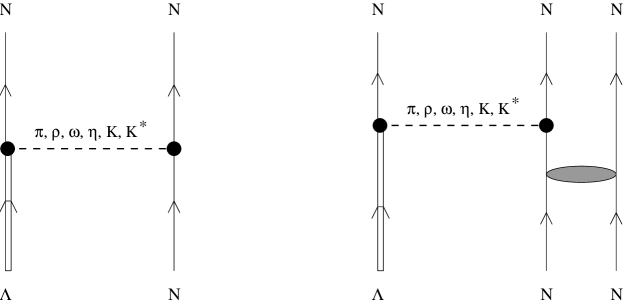
Figure 1: One–nucleon and two–nucleon induced $\Lambda$ decay in nuclei

The decay width associated to the various non-mesonic processes can be denoted as follows ($n$ indicates a neutron, $p$ a proton):

$$\Gamma_{n}:\hskip 11.38109pt\Lambda n \rightarrow nn$$ (2)

$$\Gamma_{p}:\hskip 11.38109pt\Lambda p \rightarrow np$$ (3)

$$\Gamma_{2}:\hskip 8.53581pt\Lambda NN \rightarrow NNN$$ (4)

whence the total non-mesonic width is $\Gamma_{\rm NM}=\Gamma_{1}+\Gamma_{2}\equiv\Gamma_{n}+\Gamma_{p}+\Gamma_{2}$. The total hypernuclear decay width is then:

$$\Gamma_{\rm T}=\Gamma_{\rm M}+\Gamma_{\rm NM}$$ (5)

where $\Gamma_{\rm M}=\Gamma_{\pi^{-}}+\Gamma_{\pi^{0}}$ is the mesonic width.

The non-mesonic mode can occur only in nuclei, and therefore it is the only source of information on the ${\Lambda}N\rightarrow NN$ weak interaction.

Concerning the kinematics of the process, it is worth noticing that if one assumes the $\Lambda$ at rest ($Q$-value of about 176 MeV$\simeq m_{\Lambda}-m_{N}$) and an equal share of the available energy between the two (respectively, three) final nucleons, the momenta of the emitted nucleons are expected of the order of $p_{N}\simeq 420$ MeV/c for the one-body induced decay (respectively, $p_{N}\simeq 340$ MeV/c for the two-body induced decay). Hence we do not expect a significative influence of the Pauli principle on these decay channels.

An interesting feature of the experimental decay widths of $\Lambda$-hypernuclei is the approximate stability of this quantity in passing from medium-light to very heavy systems: the mesonic ($\Gamma_{\rm M}$) and non-mesonic ($\Gamma_{\rm NM}$) partial widths depend upon the mass number in such a way as to compensate each other. This saturation property is clearly related to the short range of the ${\Lambda}N$ weak interaction.[3, 4]

2 Theoretical models for $\Lambda$-hypernuclear decay

The starting point for all methods described below is the weak effective hamiltonian for ${\Lambda}\to\pi N$ decay:

$${\mathcal{H}}^{W}_{{\Lambda}\pi N}=iGm_{\pi}^{2}\overline{\psi}_{N}(A+B\gamma_{5}){\vec{\tau}}\cdot{\vec{\phi}}_{\pi}{\psi}_{\Lambda},$$ (6)

the parameters of which are fixed on the free $\Lambda$ decay: $G=2.211\cdot 10^{-7}/m_{\pi}^{2}$, $A=1.06$ (PV amplitude) and $B=-7.10$ (PC amplitude). To enforce the $\Delta I=1/2$ rule the hyperon is assumed to be an isospin spurion with $I=1/2$, $I_{z}=-1/2$.

In the non-relativistic limit, one can then express the free $\Lambda$ decay width as follows:

$$\Gamma^{\rm free}_{\alpha}=c_{\alpha}(Gm^{2}_{\pi})^{2}\int\frac{d\vec{q}}{(2\pi)^{3}\,2\omega({\vec{q}})}\,2\pi\,$$

$$\,\quad\qquad\times\delta[E_{\Lambda}-\omega({\vec{q}})-E_{N}]\left(S^{2}+\frac{P^{2}}{m^{2}_{\pi}}{\vec{q}}^{2}\right),$$ (7)

where $c_{\alpha}=1(2)$ for $\Gamma_{\pi^{0}}$ ($\Gamma_{\pi^{-}}$, respectively) and the decay occurs both through parity violating (the s-wave amplitude, $S=A$) and parity conserving (the p-wave amplitude, $P=m_{\pi}B/(2m_{N})$) terms.

2.1 The wave function method

An expression similar to (7) for the mesonic width of hypernuclei can be obtained by explicitly taking into account the hyperon ($\phi_{\Lambda}$), pion ($\phi_{\pi}$) and nucleon ($\phi_{N}$) wave functions inside the nucleus [2, 5, 6]:

$$\!\!\!\!\!\!\Gamma_{\alpha}=c_{\alpha}(Gm^{2}_{\pi})^{2}\sum_{N\neq F}\int\frac{d\vec{q}}{(2\pi)^{3}\,2\omega({\vec{q}})}\,2\pi\,\delta[E_{\Lambda}-\omega({\vec{q}})-E_{N}]\times$$ (8)

$$\times\left\{S^{2}\left|\int d{\vec{r}}\phi_{\Lambda}(\vec{r})\phi_{\pi}({\vec{q}},{\vec{r}})\phi^{*}_{N}(\vec{r})\right|^{2}+\frac{P^{2}}{m^{2}_{\pi}}\left|\int d{\vec{r}}\phi_{\Lambda}(\vec{r}){\vec{\nabla}}\phi_{\pi}({\vec{q}},{\vec{r}})\phi^{*}_{N}(\vec{r})\right|^{2}\right\}$$

The pion wave function corresponds to an outgoing wave solution of the Klein–Gordon equation in the presence of a suitable $\pi$-nucleus optical potential, $V_{\rm opt}$, while the $\Lambda$ wave function can be derived within a variety of hypernuclear shell models, whose parameters are typically determined by comparison with the available spectroscopic data.

Turning now to the evaluation of the non-mesonic width, one needs an explitic model for the $\Lambda N\to NN$ weak transition: the latter is usually described in terms of the exchange of virtual mesons belonging to the pseudoscalar ($\pi,\eta$ and $K$) or to the vector ($\rho,\omega$ and $K^{*}$) octets. The most important (from an heuristic point of view) component of the $\Lambda N\to NN$ transition potential is associated to the exchange of a pion:

$$V_{\pi}({\vec{q}})=-Gm_{\pi}^{2}\frac{g_{NN\pi}}{2m_{N}}\left(A+\frac{B}{2\bar{m}}{\vec{\sigma}_{1}}\cdot{\vec{q}}\right)\frac{{\vec{\sigma}_{2}}\cdot{\vec{q}}}{{\vec{q}}^{2}+m_{\pi}^{2}}{\vec{\tau}_{1}}\cdot{\vec{\tau}_{2}}$$ (9)

with $\bar{m}=(m_{\Lambda}+m_{N})/2$.

This is the only component of the $\Lambda N\to NN$ meson exchange potential, for which the couplings of both the weak and strong vertices are well constrained by the existing phenomenology and experimental data. The exchange of heavier mesons, which cannot be produced in the free-$\Lambda$ weak decay, is subject to theoretical uncertainties and to a somewhat large indetermination of the model parameters (typically couplings and masses), in spite of the existence of various theoretical schemes which, in principle, should allow to fix them on a firm basis. Nevertheless the influence of $\Lambda N\to NN$ processes mediated by heavier mesons on the calculated non-mesonic decay widths appears to be important in order to reproduce the available experimental data.

A sort of “minimal model”, which has been often employed in the literature [7], accounts for the exchange of pions and $\rho$-mesons, together with phenomenological, $q$-dependent short range correlations, usually parameterized in the Landau-Migdal form (see, for details, ref. [1]).

In the framework of the wavefunction method, the one-body induced non-mesonic decay width takes the form:

$$\Gamma_{1}=\int\frac{d{\vec{p}}_{1}}{(2\pi)^{3}}\int\frac{d{\vec{p}}_{2}}{(2\pi)^{3}}\,2\pi\,\delta({\rm E.C.})\overline{{\sum}}\left|{\mathcal{M}}({\vec{p}}_{1},{\vec{p}}_{2})\right|^{2},$$ (10)

where

$${\mathcal{M}}({\vec{p}}_{1},{\vec{p}}_{2})\equiv\langle\Psi_{R};N({\vec{p}}_{1})N({\vec{p}}_{2})|\hat{T}_{\Lambda N\to NN}|\Psi_{H}\rangle$$ (11)

is the transition matrix element between the initial hypernuclear state $|\Psi_{H}\rangle$ and the final state with two outgoing nucleons, while $\delta({\rm E.C.})$ guarantees energy conservation. Besides the above mentioned uncertainties in the OME (One-Meson-Exchange) transition potential, one faces here also the complications associated with a strongly interacting many-body system.

We will not consider here further details of this method, however it is worth recalling that the wave function approach is considered to be the most appropriate one for the calculation of light $\Lambda$-hypernuclei mesonic widths; it is, instead, less accurate for the non-mesonic widths and certainly less practical for the heavier systems.

2.2 The polarization propagator method

This method obtains the hypernuclear decay width through the evaluation of the $\Lambda$ self-energy inside the nuclear medium [8, 9, 7, 10, 11]:

$${\Gamma}_{\Lambda}=-2\;{\rm Im}\,{\Sigma}_{\Lambda}\,.$$ (12)

The starting point is again the weak effective Hamiltonian (6), which provides the relevant vertices already in the simplest process illustrated in diagram (a) of Fig. 2, which corresponds to the free $\Lambda$ decay. More generally, a few contributions to the $\Lambda$ self-energy in the medium are illustrated in diagrams (b)–(h) of Fig. 2, where the pion propagator is typically dressed by the strong interaction with particle-hole (ph), $\Delta$-hole ($\Delta$h) and two particles-two holes (2p2h) intermediate states. Further contributions arise from the medium modifications on the nucleon propagator, which has origin in the $\Lambda\pi N$ weak vertex.

Figure 2: Lowest order terms for the ${\Lambda}$ self–energy in nuclear matter.

Formally the $\Lambda$ self-energy can be written as:

$${\Sigma}_{\Lambda}(k)=3i(Gm_{\pi}^{2})^{2}\int\frac{d^{4}q}{(2\pi)^{4}}\left(S^{2}+\frac{P^{2}}{m_{\pi}^{2}}\vec{q}\,^{2}\right)F_{\pi}^{2}(q)G_{N}(k-q)G_{\pi}(q)\,,$$ (13)

where $k$ is the $\Lambda$ momentum inside the nucleus, $G_{N}(p)$ and $G_{\pi}(q)$ are the nucleon and pion propagators (in nuclear matter):

$$G_{N}(p)=\frac{{\theta}(\mid\vec{p}\mid-k_{F})}{p_{0}-E_{N}(\vec{p})-V_{N}+i{\epsilon}}+\frac{{\theta}(k_{F}-\mid\vec{p}\mid)}{p_{0}-E_{N}(\vec{p})-V_{N}-i{\epsilon}}\,,$$ (14)

and

$$G_{\pi}(q)=\frac{1}{q_{0}^{2}-\vec{q}\,^{2}-m_{\pi}^{2}-{\Sigma}_{\pi}^{*}(q)}\,.$$ (15)

In equation (14) the medium effects on the nucleon propagation are phenomenologically embodied in the nuclear binding potential $V_{N}$, while in (15) the analogous effects on the pion appear in the pion self-energy, illustrated above.

More explicitly, by inserting (13) into (12), one can express the $\Lambda$-hypernuclear decay width as:

$${\Gamma}_{\Lambda}(\vec{k},\rho)=-6(Gm_{\pi}^{2})^{2}\int\frac{d\vec{q}}{(2\pi)^{3}}{\theta}(\mid\vec{k}-\vec{q}\mid-k_{F})$$

$$\,\quad\times{\theta}(k_{0}-E_{N}(\vec{k}-\vec{q})-V_{N}){\rm Im}\left[{\alpha}(q)\right]_{q_{0}=k_{0}-E_{N}(\vec{k}-\vec{q})-V_{N}}$$ (16)

where:

$${\alpha}(q)=\left(S^{2}+\frac{P^{2}}{m_{\pi}^{2}}\vec{q}\,^{2}\right)F_{\pi}^{2}(q)G_{\pi}^{0}(q)+\frac{\tilde{S}^{2}(q)U_{L}(q)}{1-V_{L}(q)U_{L}(q)}+$$

$$\,\,\quad+\frac{\tilde{P}_{L}^{2}(q)U_{L}(q)}{1-V_{L}(q)U_{L}(q)}+2\frac{\tilde{P}_{T}^{2}(q)U_{T}(q)}{1-V_{T}(q)U_{T}(q)}$$ (17)

In the above, to perform a realistic calculation, the effective interactions $\tilde{S}$, $\tilde{P}_{L}$, $\tilde{P}_{T}$,$V_{L}$, $V_{T}$ include $\pi$- and $\rho$-exchange plus short range repulsive correlations. Specifically: $V_{L}$, $V_{T}$ are the (strong) p-h interaction and include a Landau parameter $g^{\prime}(q)$, which embodies the NN short range repulsion. $\tilde{S}$, $\tilde{P}_{L}$ and $\tilde{P}_{T}$ correspond to the lines connecting the weak and strong hadronic vertices and contain another Landau parameter, $g^{\prime}_{\Lambda}(q)$ [a priori different from $g^{\prime}$], which is intended to parameterize the strong $\Lambda N$ short range correlations.

Besides the interaction lines, the other key-ingredient of (17) are the longitudinal and transverse (with respect to the pion momentum ${\vec{q}}$) polarization propagators, $U_{L}$ and $U_{T}$. They contain the Lindhard functions for p-h and ${\Delta}$-h excitations and the irreducible 2p-2h polarization propagator:

$$U_{L,T}(q)=U^{ph}(q)+U^{\Delta h}(q)+U^{2p2h}_{L,T}(q)$$ (18)

The imaginary part of $\alpha(q)$, needed to evaluate ${\Gamma}_{\Lambda}$, develops various contributions, namely:

$${\rm Im}\,\frac{U_{L,T}(q)}{1-V_{L,T}(q)U_{L,T}(q)}=\frac{{\rm Im}\,U^{ph}(q)+{\rm Im}\,U^{\Delta h}(q)+{\rm Im}\,U^{2p2h}_{L,T}(q)}{\mid 1-V_{L,T}(q)U_{L,T}(q)\mid^{2}}\,.$$ (19)

Indeed the three terms represent different decay mechanisms of the hypernucleus:

$$\Gamma_{M}\propto{\rm Im}\,U^{\Delta h}\qquad$$ (part of mesonic width)

$$\Gamma_{1}\,\propto{\rm Im}\,U^{ph}\qquad$$ (non-mesonic, one-body induced decay width)

$$\Gamma_{2}\propto{\rm Im}\,U^{2p2h}\qquad$$ (non-mesonic, two-body induced decay width

and additional part of mesonic width)

While the p-h and ${\Delta}$-h polarization propagators are well known and can be analytically evaluated [12], the 2p-2h polarization propagator, even in the non-relativistic limit considered here, demands quite a computing effort to be fully determined. On the other hand, according to the above relations, it is needed for estimating the two-body induced decay width.

In this context two approaches have been utilized till now for the evaluation of $U^{2p2h}_{L,T}(q)$:

A. Phenomenological model.
In this case one takes into account mainly the phase space available to 2p-2h excitations in nuclear matter and determines the relevant entity of the 2p-2h propagator through its connection with the phenomenological $\pi$-nucleus optical potential. The relation with specific hypernuclei is then obtained by implementing the local density approximation.

B. Microscopic calculation.
This approach proceeds through the path-integral formulation and provides the 2p-2h propagator within the so-called One Boson Loop (OBL) approximation, which embodies a rich variety of perturbative contributions to $U^{2p2h}_{L,T}(q)$.

In the following we will consider only the phenomenological approach and we refer the reader to refs. [11, 1] for the details and the results of the microscopic approach.

2.3 The phenomenological $2p2h$ propagator

In the $(q_{0},\vec{q})$ region where the p-h and $\Delta$-h excitations are off–shell, the following relation between $U^{2p2h}_{L}$ and the $p$–wave pion–nucleus optical potential $V_{\rm opt}$ holds:

$$\frac{\displaystyle\vec{q}\,^{2}\frac{f^{2}_{\pi}}{m^{2}_{\pi}}F^{2}_{\pi}(q)U^{2p2h}_{L}(q)}{\displaystyle 1-\frac{f^{2}_{\pi}}{m^{2}_{\pi}}g_{L}(q)U_{L}(q)}=2q_{0}V_{\rm opt}(q)\,.$$ (20)

At pion threshold the latter can be parameterized as:

$$2q_{0}V_{\rm opt}(q_{0}\simeq m_{\pi},\vec{q}\simeq\vec{0};\rho)=-4\pi\vec{q}\,^{2}\rho^{2}C_{0}$$ (21)

where $C_{0}$ is a complex number extracted from the experimental data on pionic atoms [13]; its “proper part” (using $g^{\prime}\equiv g_{L}(0)=0.615$) turns out to be:

$$C^{*}_{0}=(0.105+i0.096)/m^{6}_{\pi}\,.$$

Hence one obtains the following parameterization of the proper 2p-2h polarization propagator in the spin–longitudinal channel at pion threshold:

$$\vec{q}\,^{2}\frac{f^{2}_{\pi}}{m^{2}_{\pi}}F^{2}_{\pi}U^{2p2h}_{L}(q_{0}\simeq m_{\pi},\vec{q}\simeq\vec{0};\rho)=-4\pi\vec{q}\,^{2}\rho^{2}C^{*}_{0}\,.$$ (22)

Further, to obtain the general dependence of $U^{2p2h}_{L,T}$ upon $(q_{0},\vec{q})$, one considers the phase space available for the real 2p-2h excitations:

$$P(q_{0},\vec{q};\rho)\propto\int\frac{d^{4}k}{(2\pi)^{4}}\,{\rm Im}\,U^{ph}\left(\frac{q}{2}+k;\rho\right)$$

$$\quad\times{\rm Im}\,U^{ph}\left(\frac{q}{2}-k;\rho\right)\theta\left(\frac{q_{0}}{2}+k_{0}\right)\theta\left(\frac{q_{0}}{2}-k_{0}\right)\,,$$ (23)

which amounts to neglect the energy and momentum dependence of the p-h interaction. Finally the imaginary part of $U^{2p2h}_{L,T}$ will be written as:

$${\rm Im}\,U^{2p2h}_{L,T}(q_{0},\vec{q};\rho)=\frac{P(q_{0},\vec{q};\rho)}{P(m_{\pi},\vec{0};\rho_{\rm eff})}{\rm Im}\,U^{2p2h}_{L,T}(m_{\pi},\vec{0};\rho_{\rm eff})$$ (24)

with $\rho_{\rm eff}=0.75\rho$.

The above formulas refer to homogeneous nuclear matter and provide, through equations (16) and (17), the hypernuclear decay width for a $\Lambda$ with momenum $k$ embedded in a constant nuclear density $\rho$. The corresponding decay width in finite hypernuclei can be obtained by applying the local density approximation (LDA).

The latter amounts to consider a local Fermi momentum

$$k_{F}(\vec{r})=\left\{\frac{3}{2}{\pi}^{2}\rho(\vec{r})\right\}^{1/3}\,,$$ (25)

which is defined in the Thomas-Fermi approximation, as follows:

$$\epsilon_{F}(\vec{r})+V_{N}(\vec{r})\equiv\frac{k_{F}^{2}(\vec{r})}{2m_{N}}+V_{N}(\vec{r})=0.$$ (26)

The decay width in finite nuclei is then obtained by:

$${\Gamma}_{\Lambda}=\int d\vec{k}\,|\tilde{\psi}_{\Lambda}(\vec{k})|^{2}{\Gamma}_{\Lambda}(\vec{k})$$ (27)

where:

$${\Gamma}_{\Lambda}(\vec{k})=\int d\vec{r}\,|{\psi}_{\Lambda}(\vec{r})|^{2}{\Gamma}_{\Lambda}\left[\vec{k},\rho(\vec{r})\right]$$ (28)

and $|\tilde{\psi}_{\Lambda}(\vec{k})|^{2}$ is the ${\Lambda}$ momentum distribution.

3 Theory versus experiment

In the phenomenological approach for the polarization propagator we have employed the customary Fermi distribution of the nuclear density:

$$\rho_{A}(r)=\frac{\rho_{0}}{\left\{\displaystyle 1+\exp\left[\frac{r-R(A)}{a}\right]\right\}}$$ (29)

with $R(A)=1.12A^{1/3}-0.86A^{-1/3}$ fm and $a=0.52$ fm.

The ${\Lambda}$ wave function is obtained from a Woods–Saxon $\Lambda$–nucleus potential, which exactly reproduces the first two single particle eigenvalues ($s$ and $p$ $\Lambda$ levels) of the hypernucleus under analysis [10].

Short range correlations ($g^{\prime}$, $g^{\prime}_{\Lambda}$) are fixed to get agreement with experimental data: indeed the Landau parameter $g^{\prime}$ has been widely used in the literature, in connection with spin-isospin nuclear responses as measured in charge exchange reactions and inelastic electron scattering. In this context the customary value, used within the RPA framework and appropriate to fit the data is $g^{\prime}=0.6\div 0.7$.

The available data from $\Lambda$-hypernuclei decay seem to require a somewhat larger value of $g^{\prime}$ (0.8), together with $g^{\prime}_{\Lambda}\simeq 0.4$. This is not necessarily in contrast with previous phenomenology, since the RPA-type correlations are now applied to a richer polarization propagator, which also includes the 2p-2h excitations.

Figure 3: Partial ${\Lambda}$ decay widths in finite nuclei as a function of the nuclear mass number $A$. The experimental data are taken from Refs. [14, 15, 16]

In Fig. 3 we illustrate the results obtained [10] with the polarization propagator method (together with LDA) for the decay widths of various $\Lambda$-hypernuclei. In addition to the total decay rates, the mesonic and non-mesonic partial rates are shown, the latter being separated into the one-body induced ($\Gamma_{1}$) and two-body induced ($\Gamma_{2}$) decay rates. The total decay rate appears to be rather constant with the mass number, at least for $A>10$ (saturation property), as a result of a compensation between the mesonic decay and the non-mesonic one.

Altogether the results of the theoretical calculation appear to be in good agreement with the available experimental data, both on the total rates and, when available, with the non-mesonic rates. Similar outcomes, though not reported here, were obtained with the microscopic calculation of the 2p-2h polarization propagator, a fact which demonstrates how the theoretical description of these processes is well founded.

4 The $\Gamma_{n}/\Gamma_{p}$ puzzle

The main problem concerning the weak decay rates is to reproduce the experimental value for the ratio ${\Gamma}_{n}/{\Gamma}_{p}$ between the neutron– and the proton–induced widths:

$${\Lambda}n\rightarrow nn\qquad{\mathrm{and}}\qquad{\Lambda}p\rightarrow np$$ (30)

Theoretical calculations underestimate the central data for all considered hypernuclei:

$$\left\{\frac{{\Gamma}_{n}}{{\Gamma}_{p}}\right\}^{\rm Th}\ll\left\{\frac{{\Gamma}_{n}}{{\Gamma}_{p}}\right\}^{\rm Exp},\hskip 14.45377pt0.5\mathrel{\mathop{\kern 0.0pt\hbox to0.0pt{\raise 0.86108pt\hbox{$<$}\hss}}\lower 3.87495pt\hbox{\kern-1.90002pt$\sim$}}\left\{\frac{{\Gamma}_{n}}{{\Gamma}_{p}}\right\}^{\rm Exp}\mathrel{\mathop{\kern 0.0pt\hbox to0.0pt{\raise 0.86108pt\hbox{$<$}\hss}}\lower 3.87495pt\hbox{\kern-1.90002pt$\sim$}}2$$ (31)

One should keep in mind that, up to now, the data on the separate rates are limited and not precise enough, due to the difficulty in detecting the products of the non–mesonic decays, especially neutrons. The present experimental energy resolution does not allow to identify the final state of the residual nuclei in ${}^{A}_{\Lambda}{\rm Z}\rightarrow{{}^{A-2}{\rm Z}}+nn$ and ${}^{A}_{\Lambda}{\rm Z}\rightarrow{{}^{A-2}({\rm Z-1})}+np$.

In the OPE approximation, by assuming the $\Delta I=1/2$ rule in the $\Lambda\rightarrow\pi^{-}p$ and $\Lambda\rightarrow\pi^{0}n$ free couplings, many different calculations give small ratios, in the range $0.05\div 0.20$.

$$\left[\frac{\Gamma_{n}}{\Gamma_{p}}\right]^{\rm OPE}\simeq 0.05\div 0.20$$ (32)

for all the considered systems.

For pure $\Delta I=3/2$ transitions the OPE ratio can increase up to about $0.5$. However, this assuption would be inconsistent with the fact that the OPE model with $\Delta I=1/2$ couplings well reproduces the one–body stimulated non–mesonic rates $\Gamma_{1}=\Gamma_{n}+\Gamma_{p}$ for light and medium hypernuclei.

Other ingredients beyond the OPE might be responsible for the large experimental ratios:

1. Calculations with $\Lambda N\rightarrow NN$ transition potentials including heavy–meson–exchange (e.g. $K$) or direct quark contributions have improved the situation.[6, 17]

2. The analysis of the ratio ${\Gamma}_{n}/{\Gamma}_{p}$ is influenced by the two–nucleon induced process ${\Lambda}NN\rightarrow NNN$: by assuming the quasi–deuteron approximation for the absorption of the meson emitted in the $\Lambda$ decay, the three–body process are mainly ${\Lambda}np\rightarrow nnp$ and a considerable fraction of neutrons could come from this channel in addition to $\Lambda n\rightarrow nn$ and $\Lambda p\rightarrow np$. However the inclusion of the new channel would bring to extract from the experiment even larger values for the ${\Gamma}_{n}/{\Gamma}_{p}$ ratios.[9, 7]

3. The effect of the final state interaction (FSI) on the spectra of the emitted nucleons: the nucleon energy/momentum distributions have been calculated [18] by using a Monte Carlo simulation to describe the nucleon rescattering inside the nucleus. The main effects thus obtained indicate that the nuclear collisions remove nucleons from the high to the low energy part of the spectrum, moreover the numbers of emitted protons and neutrons tend to become similar (due to charge exchange processes.

A recent upgrading of the calculations quoted above shows that the experimental proton spectra are compatible with values of the ${\Gamma}_{n}/{\Gamma}_{p}$ ratio between 0.5 and 1.0, still leaving some discrepancy with the direct theoretical estimates.

5 Conclusions

It is by now well understood that beyond the mesonic channel, hypernuclear decay proceeds through non–mesonic processes, induced by one nucleon or by a pair of correlated nucleons. This channel is dominant in medium–heavy hypernuclei, where the Pauli principle strongly suppresses the mesonic decay.

The mesonic rates have been reproduced quite well by calculations performed in different frameworks. The non–mesonic rates have been considered within several phenomenological and microscopic models, most of them based on the pion exchange. More complex meson exchange potentials and direct quark models have also been used for the evaluation of non–mesonic decay rates. The obtained rates appear to be in agreement with the experimental data.

Although several calculations reproduce the total non–mesonic width, $\Gamma_{NM}=\Gamma_{n}+\Gamma_{p}(+\Gamma_{2})$, the obtained $\Gamma_{n}/\Gamma_{p}$ are often in strong disagreement with the measured central data. Hence further efforts (especially on the experimental side) must be invested in order to understand the detailed dynamics of the non–mesonic decay.

Recent experiments at KEK [19] have considerably reduced the error bars on ${\Gamma}_{n}/{\Gamma}_{p}$, by means of single nucleon spectra measurements. Good statistics coincidence measurements of $nn$ and $np$ emitted pairs are required. The angular correlation measurements, as expected from the forthcoming FINUDA [20] experiment, will also allow for the identification of nucleons coming out from the one– and two–nucleon induced processes.

References

- [1] W.M. Alberico, G. Garbarino, Phys. Rep. 369, 1 (2002).
- [2] J. Nieves, E. Oset, Phys. Rev. C 47, 1478 (1993).
- [3] J. Cohen, Prog. Part. Nucl. Phys. 25, 139 (1990).
- [4] E. Oset, A. Ramos, Prog. Part. Nucl. Phys. 41, 191 (1998).
- [5] T. Motoba, K. Itonaga, Prog. Theor. Phys. Suppl. 117, 477 (1994).
- [6] A. Parreno, A. Ramos, Phys. Rev. C 65, 015204 (2002).
- [7] A. Ramos, E. Oset, L.L. Salcedo, Phys. Rev. C 50, 2314 (1994).
- [8] E. Oset, L.L. Salcedo, Nucl. Phys. A 443, 704 (1985).
- [9] W.M. Alberico, A. De Pace, M. Ericson, A. Molinari, Phys. Lett. B 256, 134 (1991).
- [10] W.M. Alberico, A. De Pace, G. Garbarino, A. Ramos, Phys. Rev. C 61, 044314 (2000).
- [11] W.M. Alberico, A. De Pace, G. Garbarino, R. Cenni, Nucl. Phys. A 668, 113 (2000).
- [12] A.L. Fetter and J.D. Walecka, Quantum Theory of Many-particle systems, McGraw–Hill (1971).
- [13] C. Garcia-Recio, J. Nieves, E. Oset, Nucl. Phys. A 547, 473 (1992).
- [14] J.J. Szymanski, et al., Phys. Rev. C 43, 849 (1991).
- [15] T.A. Armstrong, et al., Phys. Rev. C 47, 1957 (1993).
- [16] H.C. Bhang, et al., Phys. Rev. Lett. 81, 4321 (1998).
- [17] K. Sasaki, T. Inoue, M. Oka, Nucl. Phys. A 669, 331 (2000).
- [18] A. Ramos, M.J. Vicente-Vacas, E. Oset, Phys. Rev. C 55, 735 (1997).
- [19] H.C. Bhang, et al., Nucl. Phys. A 691, 156c (2001).
- [20] T. Bressani, these Proceedings.