Super-Symmetry transformation for excitation processes

Abstract

Quantum Mechanics SUper-SYmmetry (QM-SUSY) provides a general framework for studies using phenomenological potentials for nucleons (or clusters) interacting with a core. The SUSY potentials result from the transformation of the mean field potential in order to account for the Pauli blocking of the core orbitals. In this article, we discuss how other potentials (like external probes or residual interactions between the valence nucleons) are affected by the SUSY transformation. We illustrate how the SUSY transformations induce off-diagonal terms in coordinate space that play the essential role on the induced transition probabilities on two examples: the electric operators and Gaussian external fields. We show that excitation operators, doorway states, strength and sum rules are modified.

I Introduction

Almost all branches of many-body physics have developed methods to simplify a many-body self-interacting system into a local “effective” mean potential affecting the pertinent degrees of freedom. It often provides an adequate starting point for more sophisticated approaches. For example, phenomenological potentials replacing the Schrödinger equation of N self-interacting particles by a one body potential whose orbits simulate the experimentally known structure have been widely used in nuclear physics. Of particular interest are the halo systems which are often described in terms of valence nucleons interacting with a core. An elegant way to justify the effective core-nucleon phenomenological interaction is to invoke a super-symmetric (SUSY) transformation of the mean-field potential of a N-body system Wit81 ; And84 ; Suk85 ; Bay87 ; Coo95 . Indeed, since the core is made of nucleons occupying the lowest orbitals of the mean-field potential, the halo nucleons cannot fill in these occupied states because of the Pauli exclusion principle. SUSY transformations including the forbidden states removal (States Removal Potential, SRP) and the restoration of phase shifts (Phase Equivalent Potential, PEP) provide an exact way to remove the states occupied by the core without altering the remaining states properties. Hence, SUSY transformation which can be fully analytical for some classes of potentials Coo95 , provides an equivalent effective interaction between composite systems and thus can be safely used to describe nuclear structure and reaction of nuclei presenting a high degree of clusterization.

SUSY transformations have been applied to breakup mechanisms involving halo nuclei Rid96 ; Cap03 . Indeed, the phenomenological treatment of halo nuclei in terms of nucleons in interaction with a core should take into account the fact that some intrinsic bound states of the nucleon-core potential are Pauli blocked. For instance, the $1s$ orbital is generally occupied by the core nucleons. In the case of a one neutron halo, like ¹¹Be or ¹⁹C, SUSY-PEP potentials have been used to calculate $B$(E1) matrix elements Rid96 , Coulomb breakup Cap03 , transfer reactions Gon00 . In the case of two neutrons halo, like ⁶He, ¹¹Li, or ¹⁴Be, it has been applied to remove the forbidden states and to analyze binding energies and radii of these nuclei Hes99 ; Tho00 ; Can01 ; Des03 . Finally, it has also been included in coupled-channel calculations Lee00 ; Shi00 ; Sam03 . In all these calculations, SUSY transformation has been applied considering the following approximation: only the internal part of the Hamiltonian (the core-halo potential) is SUSY transformed while the additional fields (external potentials, two-body correlations in the halo) remain unmodified. This approximation will be called the internal SUSY approximation because it concerns only the core-halo potential. In the framework of this approximation, the SUSY transformation is not equivalent to the exact treatment in which the Pauli blocked states are projected out. In this article, we discuss a consistent SUSY framework which is always equivalent to the full projection-method.

The accuracy of the internal SUSY transformation has been discussed in several papers. For instance, Ridikas et al. Rid96 have analyzed the radii of several halo nuclei as well as $B$(E1) matrix elements before and after the SUSY transformation. Thompson et al. Tho00 and Descouvemont et al. Des03 have performed a comparison of the full projector-method with the internal SUSY. As the consistent SUSY framework we discuss is totally equivalent to the full projection-method, the comparison between the internal approximation and the consistent SUSY treatment is thus an alternative method to estimate the accuracy of the internal approximation. From the theoretical point of view, the consistent SUSY approach provides a unique and exact framework to compute excitation processes or to take into account residual interaction between valence nuclei. Such a consistent framework is essential to interpret the results of inverse problems in scattering theory Cha77 .

This article is organized in the following way. In section II, we develop a consistent formalism to map the original Hamiltonian into the SUSY partner Hamiltonian. In the case of a static problem, this mapping is the usual one, but we will show in section III that in the case of an Hamiltonian modified by either an external field or a two-body interaction (for instance 2 neutrons in the halo), one should transform these fields into the new space. In section IV, we will illustrate the SUSY transformation showing both analytical results and numerical implementations for two potentials which are important in nuclear physics. We will then discuss the transformation of external field: in section V, the response to an electric excitation of the general form ${\hat{r}}^{\lambda}\hat{Y}_{LM}$, and the response to a Gaussian potential in section VI.

II SUSY transformation for one body Hamiltonian

The application of supersymmetry to Schrödinger quantum mechanics Wit81 ; And84 ; Suk85 ; Bay87 ; Coo95 has shed new light on the problem of constructing phase-equivalent potentials. In this section, we review the SUSY transformations which remove a state (SRP) and impose that the phase shifts are conserved (PEP) Bay87b ; Anc92 . We will introduce mapping operators which change the Hamiltonian as well as the bound states. Finally we will present effects on the external potential and residual interaction of composite systems described through effective Hamiltonians.

II.1 Initial Hamiltonian: $\hat{h}_{0}$

Quantum mechanics SUSY has been extensively studied for one dimensional systems. There are two ways to perform the multi-dimensional generalization depending on the choice of space coordinates. In three dimensions, one can choose the Cartesian coordinates, $(x,y,z)$ And84 or the spherical coordinates, $(r,\Omega)$ Suk85 . We choose the latter which is often used for excitation processes. Hence, the representation of the one particle Hilbert space $\mathcal{H}$ is given by a sum over the sub-spaces $\mathcal{H}^{l}$ associated to the angular momentum $l$: $\mathcal{H}=\mathcal{H}^{0}+\mathcal{H}^{1}+\mathcal{H}^{2}+\dots$

Let us introduce the initial Hamiltonian $\hat{h}_{0}$:

$$\hat{h}_{0}=\frac{\mathbf{\hat{p}}^{2}}{2m}+\mathrm{\hat{v}}_{0},$$ (1)

where $\mathbf{\hat{p}}$ is the momentum operator and where the potential operator $\mathrm{\hat{v}}_{0}$ is assumed to be local. Since $\hat{h}_{0}$ is rotationally invariant we can introduce angular momentum as good quantum number and thus the wave functions associated to an energy $E$ can be written as $\left|\phi_{0}(E)\right\rangle=\frac{1}{\hat{r}}\left|\varphi_{0}^{l}(E)\right\rangle\otimes\left|Y_{lm}\right\rangle$. In the sub-space $\mathcal{H}^{l}$, the radial static Schrödinger equation associated to the $l$th partial wave is

$$\hat{h}_{0}^{l}\left|\varphi_{0}^{l}(E)\right\rangle\equiv\left(\frac{\hat{p}^{2}}{2m}+\hat{v}_{0}^{l}\right)\left|\varphi_{0}^{l}(E)\right\rangle=E\left|\varphi_{0}^{l}(E)\right\rangle,$$ (2)

where $\hat{p}=i\hbar\;\hat{\nabla}_{r}$ is the radial momentum operator. The effective radial potential $\hat{v}_{0}^{l}$ includes the centrifugal force

$$\hat{v}_{0}^{l}=\frac{\hbar^{2}}{2m}\frac{l(l+1)}{\hat{r}^{2}}+\mathrm{\hat{v}}_{0}.$$ (3)

In order to simplify the discussion, we do not include the spin-orbit potential. Nevertheless, the generalization of this framework to include spin-orbit potential is not difficult.

In order to simplify the notations when there is no ambiguity we will drop the label $l$ since the SUSY transformations considered are defined in a subspace of angular momentum $l$ (and $m)$ $i.e.$ they are block-diagonal in the complete space. Thus, they affect differently the potential $\hat{v}^{l}$ associated with different $l$.

II.2 Hamiltonian after $k$ SUSY transformations: $\hat{h}_{k}$

The elementary SUSY transformations remove a single state with or without restoring the phase shifts. In order to remove several states we will iterate the SUSY transformation. Therefore, let us assume that after $k$ transformations the radial static Schrödinger equation associated to the $l$th partial wave can be written as

$$\hat{h}_{k}^{l}\left|\varphi_{k}^{l}(E)\right\rangle\equiv\left(\frac{\hat{p}^{2}}{2m}+\hat{v}_{k}^{l}\right)\left|\varphi_{k}^{l}(E)\right\rangle=E\left|\varphi_{k}^{l}(E)\right\rangle.$$ (4)

It should be noticed that, since the SUSY transformations are block-diagonal and different in each subspace of angular momentum $l,$ the different radial potentials do not correspond to the same potential $i.e.$ the various $\mathrm{\hat{v}}_{k}^{l}$ are different

$$\mathrm{\hat{v}}_{k}^{l}=\hat{v}_{k}^{l}-\frac{\hbar^{2}}{2m}\frac{l(l+1)}{\hat{r}^{2}}$$ (5)

for different angular momenta $l$. We call $E_{k}^{(i)}$ ($i=n,l$) the energy of the $i$th bound state of $\hat{h}_{k}^{l}$ which is thus $(2l+1)$-fold degenerate.

The bound states correspond to the square integrable solutions of the differential equation (Eq. 4). However, we will not restrict the solution of Eq. 4 to bound states but rather consider all solutions $\left|\varphi_{k}(E)\right\rangle$. Given a particular solution $\left|\widetilde{\varphi}_{k}(E)\right\rangle$ of Eq. 4 whose inverse is square integrable, the general solution of Eq. 4 can be recast as Suk85

$$\varphi_{k}(E,\alpha;r)=\widetilde{\varphi}_{k}(E;r)\left(1+\alpha\int_{r}^{\infty}\frac{dr^{\prime}}{\left(\widetilde{\varphi}_{k}(E;r^{\prime})\right)^{2}}\right),$$ (6)

where the parameter $\alpha$ can vary freely to construct all the possible solutions of the second-order differential equation (Eq. 4). In Eq. 6, we use the r-representation and the Dirac notations: $\widetilde{\varphi}_{k}(E;r)=\left\langle r\left|\widetilde{\varphi}_{k}(E)\right.\right\rangle$. For future use let us define the constant $\beta=\Big{(}\int_{0}^{\infty}dr/[\widetilde{\varphi}_{k}(E;r)]^{2}\Big{)}^{-1}$.

The Hamiltonians $\hat{h}_{k}$ can always be factorized

$$\hat{h}_{k}={\hat{a}}_{k}^{+}{\hat{a}}_{k}^{-}+\mathcal{E}_{k},$$ (7)

where $\mathcal{E}_{k}$ is the factorization energy and the first-order differential operators ${\hat{a}}{{}_{k}^{\pm}}$ (${\hat{a}}{{}_{k}^{-}}=\left({\hat{a}}{{}_{k}^{+}}\right)^{\dagger}$) are of the following form:

$${\hat{a}}{{}_{k}^{\pm}}=\frac{1}{\sqrt{2m}}\left(\hbar\hat{w}_{k}\mp i\hat{p}\right).$$ (8)

where $\hat{w}_{k}\equiv w_{k}(\hat{r})$ is the super-potential. Notice that in the literature, capital letters are usually used for the differential operators $\hat{a}_{k}^{\pm}$. Here, we dedicate capital letters for many-body operators while lower case letters are used for one-body operator. It is possible to show that the general solution $\left|\varphi_{k}(\mathcal{E}_{k},\alpha)\right\rangle$ of Eq. 4 with $E=\mathcal{E}_{k}$ is equivalently the solution of the first order differential equation

$${\hat{a}}_{k}^{-}\left|\varphi_{k}(E=\mathcal{E}_{k},\alpha)\right\rangle=0.$$ (9)

As a consequence, the super-potential is the local operator defined by

$$w_{k}(E=\mathcal{E}_{k},\alpha;r)=\frac{d}{dr}\ln\varphi_{k}(E=\mathcal{E}_{k},\alpha;r).$$ (10)

For a given factorization energy $\mathcal{E}_{k}$, there is a family of solutions which depends on the parameter $\alpha$ generating the super-potential $\hat{w}_{k}(E=\mathcal{E}_{k},\alpha)$. Note that $\varphi_{k}(E=\mathcal{E}_{k},\alpha;r)$ must be nodeless in order $\hat{a}_{k}^{\pm}$ to be bound. Hence $\mathcal{E}_{k}$ must be less than or equal to the ground state energy $E_{k}$ of $\hat{h}_{k}$ and this requires also that $\alpha>-\beta$. The choice of the factorization energy $\mathcal{E}_{k}$ and the selection of a member from the family of solutions $w_{k}$ must clearly be physically motivated.

In this section we have defined the notations used in the following. In the next section we will present a 2 step method which removes the lowest-energy state and preserves the phase shifts.

II.3 State Removal Potential (SRP): $\hat{v}_{k+1}$

The SRP transformation is defined so that it removes the lowest-energy state of a given sub-space $\mathcal{H}^{l}$. For the given angular momentum $l$, we choose $\mathcal{E}_{k}=E_{k}^{0}$, the energy of the lowest energy state of the Hamiltonian $\hat{h}_{k}$. It follows that the inverse of the particular solution is not square integrable and it imposes $\alpha$=0. With these definitions, we associate to $\hat{h}_{k}$ a supersymmetric partner $\hat{h}_{k+1}$ defined by

$$\hat{h}_{k+1} = {\hat{a}}_{k}^{-}{\hat{a}}_{k}^{+}+\mathcal{E}_{k}=\frac{\hat{p}^{2}}{2m}+\hat{v}_{k+1},$$ (11)

$$\hat{v}_{k+1} = \hat{v}_{k}-\frac{\hbar^{2}}{m}\left(\partial_{r}\;\hat{w}_{k}(\mathcal{E}_{k},\alpha=0)\right).$$ (12)

The Hamiltonians $\hat{h}_{k}$ and $\hat{h}_{k+1}$ share the same spectrum except for the lowest-energy state of $\hat{h}_{k}$ which has been suppressed in $\hat{h}_{k+1}$. The states ($\left|\varphi_{k+1}(E)\right\rangle$) of $\hat{h}_{k+1}$ can be obtained from those ($\left|\varphi_{k}(E)\right\rangle$) of $\hat{h}_{k}$ according to

$$\left|\varphi_{k+1}(E)\right\rangle=\frac{1}{\sqrt{\hat{h}_{k+1}-\mathcal{E}_{k}}}{\hat{a}}{{}_{k}^{-}}\left|\varphi_{k}(E)\right\rangle\equiv{\mathrm{\hat{u}}}_{k}^{-}\left|\varphi_{k}(E)\right\rangle.$$ (13)

Conversely, except for the ground state, the states of $\hat{h}_{k}$ can be obtained from those of $\hat{h}_{k+1}$ by

$$\left|\varphi_{k}(E)\right\rangle=\frac{1}{\sqrt{\hat{h}_{k}-\mathcal{E}_{k}}}{\hat{a}}{{}_{k}^{+}}\left|\varphi_{k+1}(E)\right\rangle={\mathrm{\hat{u}}}_{k}^{+}\left|\varphi_{k+1}(E)\right\rangle.$$

In these equations, we have introduced the pseudo unitary SRP-operators $\hat{\mathrm{u}}{{}_{k}^{-}}$ and $\hat{\mathrm{u}}{{}_{k}^{+}}$ which are defined as (the products ${\hat{a}}{{}_{k}^{+}}{\hat{a}}{{}_{k}^{-}}$ and ${\hat{a}}{{}_{k}^{-}}{\hat{a}}{{}_{k}^{+}}$ being definite positive)

$$\mathrm{\ }\hat{\mathrm{u}}{{}_{k}^{+}} = {\hat{a}}{{}_{k}^{+}}\frac{1}{\sqrt{{\hat{a}}{{}_{k}^{-}}{\hat{a}}{{}_{k}^{+}}}}=\frac{1}{\sqrt{{\hat{a}}{{}_{k}^{+}}{\hat{a}}{{}_{k}^{-}}}}{\hat{a}}{{}_{k}^{+}},$$ (14)

$$\mathrm{\ }\hat{\mathrm{u}}{{}_{k}^{-}} = {\hat{a}}{{}_{k}^{-}}\frac{1}{\sqrt{{\hat{a}}{{}_{k}^{+}}{\hat{a}}{{}_{k}^{-}}}}=\frac{1}{\sqrt{{\hat{a}}{{}_{k}^{-}}{\hat{a}}{{}_{k}^{+}}}}{\hat{a}}{{}_{k}^{-}}.$$ (15)

These operators are pseudo-unitary since $\hat{\mathrm{u}}{{}_{k}^{-}=(\hat{\mathrm{u}}{{}_{k}^{+}})}^{\dagger}$, $\hat{\mathrm{u}}{{}_{k}^{-}}\hat{\mathrm{u}}{{}_{k}^{+}}=\hat{1}$ and $\hat{\mathrm{u}}{{}_{k}^{+}}\hat{\mathrm{u}}{{}_{k}^{-}}=\hat{p}$, where the projector $\hat{p}$ suppresses the lowest-energy state $|\varphi_{k}^{0}\rangle$ of the Hamiltonian $\hat{h}_{k}$ from the sub-space $\mathcal{H}^{l}$ and can be written as $\hat{p}=1-|\varphi_{k}^{0}\rangle\langle\varphi_{k}^{0}|$.

The relation between $\hat{h}_{k}$ and $\hat{h}_{k+1}$ is

$$\hat{h}_{k+1}=\frac{\hat{p}^{2}}{2m}+\hat{v}_{k+1}=\hat{\mathrm{u}}_{k}^{+}\,\left(\frac{\hat{p}^{2}}{2m}+\hat{v}_{k}\right)\,\hat{\mathrm{u}}_{k}^{-}=\hat{\mathrm{u}}_{k}^{+}\,\hat{h}_{k}\,\hat{\mathrm{u}}_{k}^{-}$$ (16)

However, it is important to remark that $\hat{v}_{k+1}\neq\hat{\mathrm{u}}_{k}^{+}\hat{v}_{k}\hat{\mathrm{u}}_{k}^{-}$ and $\hat{p}^{2}\neq\hat{\mathrm{u}}_{k}^{+}\hat{p}^{2}\hat{\mathrm{u}}_{k}^{-}$. In fact the SUSY transformation of a local potential is not local. The simple diagonal form of the potential Eq. 12 is recovered because, by construction, the modifications of the kinetic part just cancel the off-diagonal terms in the transformed potential. Then, the kinetic and the potential parts of the Hamiltonian should be transformed together in order to get the relation (16) with a simple potential (local in the $r$-space) and kinetic (diagonal in the $p$-representation) terms.

II.4 Phase Equivalent Potential (PEP): ${\underline{v}}_{k+1}$

It can be shown that SRP transformations change the phase shifts. To solve this problem, Baye Bay87 has proposed to perform a second SUSY transformation and associate to $\hat{h}_{k+1}$ a new supersymmetric partner $\hat{{\underline{h}}}_{k+1}$ so that

$$\hat{{\underline{h}}}_{k+1}=\hat{{\underline{a}}}_{k}^{-}\hat{\underline{a}}_{k}^{+}+{\underline{{\cal E}}}_{k}=\frac{\hat{p}^{2}}{2m}+\hat{\underline{v}}_{k+1},\\ ,$$ (17)

with ${\underline{{\cal E}}}_{k}=E_{k}^{0}$, the ground state energy of $\hat{h}_{k}$, and $\alpha=-\beta$. In this case, the solution $\underline{\varphi}_{k+1}$ of $\hat{h}_{k+1}$ and its inverse are not square integrable. The second SUSY transformation does not suppress nor add any state to the spectrum of $\hat{h}_{k+1}$, but it restores the phase shifts so that the Hamiltonian $\hat{{\underline{h}}}_{k+1}$ is equivalent to $\hat{h}_{k}$ as far as the scattering properties are concerned. Note that the energy ${\underline{{\cal E}}}_{k}=E_{k}^{0}$ is now below the ground state energy $E_{k+1}^{0}$ of $\hat{h}_{k+1}$.

The corresponding super-potential $\hat{{\underline{w}}}_{k}({\underline{{\cal E}}}_{k})$ is deduced from the ground state wave function $|\varphi_{k}^{0}\rangle$ of $\hat{h}_{k+1}$ according to Eq. 10. It can also be deduced from the ground state of $\hat{h}_{k}$ according to Bay87b :

$${\underline{w}}_{k}({\underline{{\cal E}}}_{k};r) = \frac{d}{dr}\ln\frac{1}{\varphi_{k}^{0}(r)}\int_{0}^{r}dr^{\prime}\,\left(\varphi_{k}^{0}(r^{\prime})\right)^{2}$$ (18)

$$= \underline{\underline{w}}_{k}({\underline{{\cal E}}}_{k};r)-w_{k}({\mathcal{E}}_{k};r),$$

where we have used the relation $\underline{\cal E}_{k}=\mathcal{E}_{k}$ and introduced the modified-super-potential $\underline{{\underline{w}}}_{k}({\underline{{\cal E}}}_{k};r)$ as

$$\underline{\underline{w}}_{k}({\underline{{\cal E}}}_{k};r)=\frac{d}{dr}\ln\int_{0}^{r}dr^{\prime}\,\left(\varphi_{k}^{0}(r^{\prime})\right)^{2}.$$ (19)

The corresponding potential $\hat{{\underline{v}}}_{k+1}$ is

$$\hat{{\underline{v}}}_{k+1} = \hat{v}_{k+1}-\frac{\hbar^{2}}{m}\left(\partial_{r}\;\hat{\underline{w}}_{k}({\underline{{\cal E}}}_{k})\right)$$ (20)

$$= \hat{v}_{k}-\frac{\hbar^{2}}{m}\left(\partial_{r}\;\hat{\underline{\underline{w}}}_{k}({\underline{{\cal E}}}_{k})\right).$$

According to the above discussion, the spectra of $\hat{h}_{k+1}$ and $\hat{{\underline{h}}}_{k+1}$ are identical. All the states of $\hat{h}_{k}$, except its lowest-energy state, are mapped onto the states of $\hat{{\underline{h}}}_{k+1}$ with the same phase shifts. This mapping is simply:

$$\left|\underline{\varphi}_{k+1}(E)\right\rangle\!\! = \!\!\frac{1}{E_{k}^{0}-\hat{{\underline{h}}}_{k+1}}{\hat{\underline{a}}}{{}_{k}^{-}}{\hat{a}}{{}_{k}^{-}}\left|\varphi_{k}(E)\right\rangle\equiv\hat{\mathrm{\underline{u}}}{{}_{k}^{-}}\left|\varphi_{k}^{l}(E)\right\rangle,$$

$$\left|\varphi_{k}(E)\right\rangle\!\! = \!\!\frac{1}{E_{k}^{0}-\hat{h}_{k}}\hat{a}{{}_{k}^{+}}{\hat{\underline{a}}}{{}_{k}^{+}}\left|\underline{\varphi}_{k+1}(E)\right\rangle=\hat{\mathrm{\underline{u}}}{{}_{k}^{+}}\left|\underline{\varphi}_{k+1}(E)\right\rangle,$$

with the pseudo-unitary PEP-operators

$$\hat{\mathrm{\underline{u}}}_{k}^{+} = -\hat{a}_{k}^{+}\hat{\underline{a}}_{k}^{+}\frac{1}{\hat{\underline{a}}_{k}^{-}\hat{\underline{a}}_{k}^{+}}=-\frac{1}{\hat{a}_{k}^{+}\hat{a}_{k}^{-}}\hat{a}_{k}^{+}\hat{\underline{a}}_{k}^{+},$$

$$\hat{\mathrm{\underline{u}}}_{k}^{-} = -\frac{1}{\hat{\underline{a}}_{k}^{-}\hat{\underline{a}}_{k}^{+}}\hat{\underline{a}}_{k}^{-}\hat{a}_{k}^{-}=-\hat{\underline{a}}_{k}^{-}\hat{a}_{k}^{-}\frac{1}{\hat{a}_{k}^{-}\hat{a}_{k}^{+}},$$

The relation between $\hat{h}_{k}$ and $\hat{\underline{h}}_{k+1}$ is

$$\hat{\underline{h}}_{k+1}=\hat{\mathrm{\underline{u}}}_{k}^{+}\,\hat{h}_{k}\,\,\hat{\mathrm{\underline{u}}}_{k}^{-}.$$ (25)

The advantage of using the operators $\hat{u}_{k}^{\pm}$ and $\hat{\underline{u}}_{k}^{\pm}$ is that all the relations we will deduce hereafter will be algebraically equivalent for SRP and PEP transformations. In the following, as long as no confusion is possible, we will write the relations fulfilled by the general operator $\hat{u}_{k}^{\pm}$, which can be replaced either by the operator $\hat{u}_{k}^{\pm}$ for the SRP transformation or $\hat{\underline{u}}_{k}^{\pm}$ for the PEP one.

III SUSY transformation for general Hamiltonians

In nuclear physics, we are often interested in the description of $\mathrm{A}$ interacting nucleons assuming that these nucleons can be separated into a frozen core containing $\mathrm{A}_{\mathrm{c}}$ nucleons and a valence space containing $\mathrm{A}_{\mathrm{v}}$ nucleons. Hence, the wave function of this system is assumed to factorize into a core and a valence part, $\left|\Phi(\mathrm{A}_{\mathrm{c}}+\mathrm{A}_{\mathrm{v}})\right\rangle=\left|\Phi_{\mathrm{c}}(\mathrm{A}_{\mathrm{c}})\right\rangle\otimes\left|\Phi_{\mathrm{v}}(\mathrm{A}_{\mathrm{v}})\right\rangle$. The core state is described at the mean field level as a Slater determinant of $\mathrm{A}_{\mathrm{c}}$ single particle states $\left|\phi_{\mathrm{c}}(n)\right\rangle$ occupying the $\mathrm{A}_{\mathrm{c}}$ lowest-energy eigenstates of the mean field potential $\hat{h}_{0}$: $\left|\Phi_{\mathrm{c}}(\mathrm{A}_{\mathrm{c}})\right\rangle=\widetilde{\prod_{n=1}^{\mathrm{A}_{\mathrm{c}}}\left|\phi_{c}(n)\right\rangle}$ where $\widetilde{...}$ stands for the antisymmetrization sign. As a consequence of the Pauli principle, the valence nucleons cannot occupy the lowest orbitals of the core-valence potential which are already occupied by the core nucleons. The evolution of $\left|\Phi_{\mathrm{v}}(\mathrm{A}_{\mathrm{v}})\right\rangle$ is thus ruled by the Hamiltonian $\hat{H}_{\mathrm{v}}$ which contains a projection out of the occupied space $\hat{\mathrm{P}}_{\mathrm{v}}=\prod_{n=1}^{\mathrm{A}_{\mathrm{c}}}\hat{c}_{n}$ $\hat{c}_{n}^{+}$ where $\hat{c}_{n}^{+}$ ($\hat{c}_{n}$) is the creation (annihilation) operator of a nucleon in the occupied orbital $\left|\phi_{\mathrm{c}}(n)\right\rangle$. $\hat{H}_{\mathrm{v}}$ is assumed to contain the confining effect of the mean field $\hat{h}_{0}$. For cases with several nucleons in the valence space, the residual interaction among valence nucleons, $\hat{V}_{0}$ should be taken into account when the problem of correlations is addressed. Finally, an external field, $\hat{f}_{0}$, should be introduced in order to compute excitation properties. Then the Hamiltonian reads

$$\hat{H}_{\mathrm{v}}=\hat{\mathrm{P}}_{\mathrm{v}}\hat{H}\hat{\mathrm{P}}_{\mathrm{v}}$$ (26)

with

$$\hat{H}=\sum_{i=1}^{\mathrm{A}_{\mathrm{v}}}\hat{h}_{0}(i)+\frac{1}{2}\sum_{i,j=1}^{\mathrm{A}_{\mathrm{v}}}\hat{V}_{0}(i,j)+\sum_{i=1}^{\mathrm{A}_{\mathrm{v}}}\hat{f}_{0}(i).$$ (27)

In the following, we propose to generalize the SUSY transformation so that it remains totally equivalent to the projector method for every kind of additional potentials. The first step of this method is to remove the $k$ orbitals occupied by the core nucleons. We introduce the full operator $\hat{\mathrm{U}}_{k-1}^{\pm}$ which is the product of the different transformations $\hat{\mathrm{u}}_{k-1}^{\pm}$ (c.f. Eq. 14 and Eq. LABEL:eq40)

$$\hat{\mathrm{U}}_{k-1}^{{}^{\pm}}=\prod_{i=1}^{\mathrm{A}_{\mathrm{v}}}\hat{\mathrm{u}}_{k-1}^{{}^{\pm}}(i)$$ (28)

applying to each single particle wave function $(i)$ of the valence state. Since those different transformations affects only a given single-particle angular-momentum subspace, the total operator $\hat{\mathrm{U}}_{k}^{{}^{\pm}}$ is block diagonal in spin representation. Being the product of pseudo-unitary transformations, $\hat{\mathrm{U}}_{k}^{{}^{\pm}}$ is also pseudo-unitary since $\hat{\mathrm{U}}_{k}^{-}=\left(\hat{\mathrm{U}}_{k}^{+}\right)^{\dagger}$, $\hat{\mathrm{U}}_{k}^{-}\hat{\mathrm{U}}_{k}^{+}=\hat{1}$ and $\hat{\mathrm{U}}_{k}^{+}\hat{\mathrm{U}}_{k}^{-}=\hat{\mathrm{P}}_{\mathrm{v}}$. Using $\hat{\mathrm{U}}_{k}^{+}\hat{\mathrm{U}}_{k}^{-}=\mathrm{\hat{P}}_{\mathrm{v}}$, we can thus write $\hat{H}_{\mathrm{v}}=\mathrm{\hat{P}}_{\mathrm{v}}\hat{H}\mathrm{\hat{P}}_{\mathrm{v}}$ and explicitly

$$\hat{H}_{\mathrm{v}}=\hat{\mathrm{U}}_{k-1}^{+}\hat{\mathrm{U}}_{k-1}^{-}H\hat{\mathrm{U}}_{k-1}^{+}\hat{\mathrm{U}}_{k-1}^{-}=\hat{\mathrm{U}}_{k-1}^{+}\hat{H}_{\mathrm{v},k}\hat{\mathrm{U}}_{k-1}^{-}$$ (29)

where we have introduced the transformed Hamiltonian

$$\hat{H}_{\mathrm{v},k} = \hat{\mathrm{U}}_{k-1}^{-}\hat{H}\hat{\mathrm{U}}_{k-1}^{+}$$ (30)

$$= \sum_{i=1}^{\mathrm{A}_{\mathrm{v}}}\hat{h}_{k}(i)+\frac{1}{2}\sum_{i,j=1}^{\mathrm{A}_{\mathrm{v}}}\hat{V}_{k}(i,j)+\sum_{i=1}^{\mathrm{A}_{\mathrm{v}}}\hat{f}_{k}(i).$$

It is clear from this relation that not only $\hat{h}_{0}$ is transformed but also the two body interaction is changed into $\hat{V}_{k}(i,j)$. Using Eq. 28 and $\hat{\mathrm{u}}_{k}^{-}\left(i\right)\hat{\mathrm{u}}_{k}^{+}\left(i\right)=\hat{1}\left(i\right)$ we get

$$\hat{V}_{k}(i,j) = \hat{\mathrm{U}}_{k-1}^{-}\hat{V}_{0}(i,j)\hat{\mathrm{U}}_{k-1}^{+}$$

$$= \hat{\mathrm{u}}_{k-1}^{-}(i)\hat{\mathrm{u}}_{k-1}^{-}(j)\hat{V}_{0}(i,j)\hat{\mathrm{u}}_{k-1}^{+}(i)\hat{\mathrm{u}}_{k-1}^{+}(j)$$

and the external potential $\hat{f}_{0}$ is mapped into

$$\hat{f}_{k}(i)=\hat{\mathrm{U}}_{k-1}^{-}\hat{f}_{0}(i)\hat{\mathrm{U}}_{k-1}^{+}=\hat{\mathrm{u}}_{k-1}^{-}(i)\hat{f}_{0}(i)\hat{\mathrm{u}}_{k-1}^{+}(i).$$ (33)

Note that when $\hat{f}_{0}$ is not a scalar operator, the mapping operator $\hat{\mathrm{u}}_{k-1}^{\pm}$ on the right and on the left of Eq. 33 may not correspond to the same angular momentum $l$.

It should also be noticed that not only the Hamiltonian is changed but also the wave functions since the state of the valence nucleons is transformed into

$$\left|\Phi_{\mathrm{v},k}\left(t\right)\right\rangle=\hat{\mathrm{U}}_{k-1}^{-}\left|\Phi_{\mathrm{v}}\left(t\right)\right\rangle.$$ (34)

The evolution of a state $|\Phi_{\mathrm{v}}(t)\rangle$ is driven by the time dependent Schrödinger equation

$$i\hbar\frac{d}{dt}\left|\Phi_{\mathrm{v}}(t)\right\rangle=\hat{H}_{\mathrm{v}}\left|\Phi_{\mathrm{v}}(t)\right\rangle,$$

which can be mapped into the new Hilbert space where the Pauli-blocked states have been removed within SUSY transformations:

$$i\hbar\frac{d}{dt}\left|\Phi_{\mathrm{v},k}(t)\right\rangle=\hat{H}_{\mathrm{v},k}\left|\Phi_{\mathrm{v},k}(t)\right\rangle.$$

It is important to remark that the projectors $\hat{P}_{\mathrm{v}}$ involved in the definition of the valence Hamiltonian (cf Eq. 27) have been removed in the mapped Hamiltonian $\hat{H}_{\mathrm{v},k}$ (cf Eq. 30). Hence, the time dependent Schrödinger equation in the SUSY space is simpler than the original Schrödinger equation which involves projection operators. Nevertheless, the two Schrödinger equations written in the original space or in the SUSY transformed Hilbert space contain strictly the same physical ingredients and are mathematically equivalent.

In the literature, the transformation of both the excitation operators and the wave functions are usually neglected i.e. $\hat{f}_{0}$ is often used instead of $\hat{f}_{k}$ and the wave functions are not transformed back when evaluating observables Rid96 ; Cap03 ; Gon00 ; Hes99 ; Tho00 ; Can01 ; Lee00 ; Shi00 ; Sam03 . In the following, we will study a particularly important application which is the evaluation of the response of the nucleus to an external (one body) perturbation (time dependent or not). The use of a SUSY transformed two body residual-interaction in the calculation of correlations and reactions will be the subject of forthcoming studies.

IV Examples of SUSY transformations

In this section, we illustrate the formalism developed above with two important physical examples: i) the harmonic oscillator potential which is mostly analytical, it allows a deeper insight into the formalism and provides numerical tests, and ii) the halo nuclei potential which are of important physical interest but can be treated only numerically since only asymptotic relations can be deduced analytically.

IV.1 The harmonic oscillator potential

The harmonic oscillator potential is a textbook example Law80 . We set the local potential to be $V_{0}(r)=-V_{0}+\frac{\hbar^{2}}{2m}(r/b)^{2}$ with $b^{2}=\hbar/m\omega$. In the following, we introduce a reduced coordinate $q=r/b.$

The eigenstates are labeled with the quantum numbers $(n,l)$ and are associated with a set of energies $E_{nl}=-V_{0}+(2n+l+3/2)\hbar\omega$. For each $l$ the lowest energy state is

$$\varphi_{0}^{0l}(q)=c_{l}\,q^{l+1}\,\exp\{-\frac{1}{2}q^{2}\},$$

with $c_{l}=b^{l-1/2}/\pi^{3/4}$.

We deduce the super-potentials for SRP and PEP transformations:

$$w_{0}^{l}(q) = \frac{1}{b}\left(\frac{l+1}{q}-q\right),$$ (35)

$$\underline{\underline{w}}_{0}^{l}(q) = \frac{1}{b}\frac{q^{2l+2}\,{\hbox{e}}^{-q^{2}}}{\mathrm{erf}(q,2l+2)},$$ (36)

with the unnormalized error function defined by $\mathrm{erf(z,l)=\int_{0}^{z}t^{l}\hbox{e}^{-t^{2}}dt}$. The differential operators $\hat{a}_{k}^{l^{\pm}}$ are

$$\langle r|\hat{a}_{0}^{l^{\pm}}|r^{\prime}\rangle = -\langle r|\frac{1}{\sqrt{2}}\left(\hat{\mathrm{r}}\pm i\hat{\mathrm{p}}-\hbar\omega\frac{l+1}{\hat{\mathrm{r}}}\right)|r^{\prime}\rangle,$$ (37)

$$\langle r|\hat{\underline{a}}_{0}^{l^{\pm}}|r^{\prime}\rangle \stackrel{{\scriptstyle\infty}}{{\sim}} -\langle r|\frac{1}{\sqrt{2}}\left(-\hat{\mathrm{r}}\pm i\hat{\mathrm{p}}\right)|r^{\prime}\rangle,$$ (38)

where $\hat{\mathrm{r}}=\sqrt{m}\omega\hat{r}$ and $\hat{\mathrm{p}}=\hat{p}/\sqrt{m}$. Notice that PEP transformation is not physical in this case because there are no phase for the harmonic oscillator potential. Nevertheless, it remains interesting for the discussion.

From the expressions of the super-potentials removing only one state, we deduce the transformed potentials:

$$v_{1}^{l}(r) = v_{0}^{l}(r)+\hbar\omega+\frac{\hbar^{2}(l+1)}{mr^{2}}=v_{0}^{l+1}(r)+\hbar\omega,$$ (39)

$${\underline{v}}_{1}^{l}(r) = v_{0}^{l}(r)+\frac{\hbar^{2}}{mb^{2}}\frac{q^{2l+1}{\hbox{e}}^{-q^{2}}}{\left({\mathrm{erf}}(q,2l+2)\right)^{2}}\times$$ (40)

$$\left((2l+2-2q^{2}){\mathrm{erf}}(q,2l+2)+q^{2l+3}\right).$$

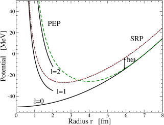
Figure 1: (color online) Radial part of the Harmonic Oscillator potential (H-O) for l=0,1,2 (thick lines) compared with its SRP (dotted line) and PEP (dashed line) transformation of the l=0 potential. The thin solid line stands for $v_{\mathrm{H-O}}(l=1)+\hbar\omega$.

These potentials are represented in Fig. 1. In the graphical illustrations we will use nuclear physics scales by taking the following parameters: $V_{0}$=50 MeV and $\hbar\omega$=10 MeV. The lowest energy state is at -35 MeV. The r.h.s. of Eq. 39 demonstrates that the SRP transformations removing only one state have mapped the original potential $v_{0}^{l}$ into a new potential which is simply $v_{0}^{l^{\prime}}+\hbar\omega$ where the effective angular momentum is $l^{\prime}=l+1$. This is illustrated in Fig. 1 where we have represented the original potential with $l=0$, $l=1$ and $l=2$ (thick lines) and the SRP potential obtained numerically (dotted line). These numerical results have been obtained on a mesh containing 400 points, ranging from 0 fm to 20 fm and with a vanishing boundary condition. The thin solid line is the analytical result given by Eq. 39. The slight difference between the thin solid line and the dotted line gives an estimate of the error of the numerical algorithm which appears to be very small.

Generalizing this result to the removal of several core states we remark that, in the new radial Hilbert space, up to a translation of $n_{c}\,\hbar\omega,$ where $n_{c}$ is the number of removed core orbitals with the angular momentum $l,$ the Pauli principle maps the original potential with angular momentum $l$ to a new potential analogous to the radial potential with an effective angular momentum $l^{\prime}=l+n_{c}$. However, only the radial wave function is affected by the effective angular momentum, the angular part of the wave function is unchanged by the SUSY mapping.

As we have already mentioned, this SRP transformation changes the phases. The restoration of the phases is ensured by the PEP transformation. From the analytic expression of ${\underline{v}}_{1}^{l}$ (Eq. 40), we see that near $r\sim 0$ , ${\underline{v}}_{1}^{l}(r)\stackrel{{\scriptstyle 0}}{{\sim}}v_{0}^{l+2}(r)$, and asymptotically, ${\underline{v}}_{1}^{l}(r)\stackrel{{\scriptstyle\infty}}{{\sim}}v_{0}^{l}(r)$. The potential ${\underline{v}}_{1}^{l}(r)$ is represented in Fig. 1 (dashed line). The restoration of the phases imposes a non trivial transformation of the potential: near zero, the potential ${\underline{v}}_{1}$ is mapped to a new potential analogous to $v_{0}^{l^{\prime}}$ with a centrifugal force analogous to an effective angular momentum $l^{\prime}=l+2n_{c}$, and asymptotically, the potential stays unchanged as required by the phase conservation. This behavior is the consequence of the Pauli principle and phase restoration.

The mapping operators, $\hat{\mathrm{u}}_{0}^{l\,\pm}$, can also be analytically derived, and we will discuss the properties of these operators from their asymptotic (all radii going to infinity) expressions:

$$\langle r|\mathrm{u}_{0}^{l+}|r^{\prime}\rangle \stackrel{{\scriptstyle\infty}}{{\sim}} -\langle r|\frac{1/\sqrt{2}}{\sqrt{\hat{p}^{2}/2m-E_{0}^{0}}}\left(i\hat{\mathrm{p}}+\hat{\mathrm{r}}\right)|r^{\prime}\rangle$$ (41)

$$\langle r|\mathrm{\underline{u}}_{0}^{l\,\pm}|r^{\prime}\rangle \stackrel{{\scriptstyle\infty}}{{\sim}} \delta(r-r^{\prime})$$ (42)

Hence, while the operator $\hat{\mathrm{u}}_{0}^{l\,\pm}$ is never trivial even at large distances the operator $\hat{\mathrm{\underline{u}}}_{0}^{l\,\pm}$ is simply the unity operator for large r. This is a consequence of the phase restoration. As a consequence, the PEP transformations do not modify observables which are only sensitive to the asymptotic part of the wave functions. These asymptotic properties are also valid for other potentials as illustrated for halo nuclei potential in the next paragraph.

IV.2 Halo nuclei potentials

The study of the properties of weakly bound systems has found a renewed interest after the discovery of halo nuclei tan85 . These systems have very large mean square radii and small separation energies. In fact, the separation energy of the nucleons forming the halo is so small that their degrees of freedom can be separated from those of the nucleons constituents of the core. Up to now, this property has been observed in light nuclei close to the nucleon drip-lines like ⁶He, ¹¹Be or ¹⁹C. In reference Gre97 , the proposed core-halo potential for ¹¹Be is the sum of a Wood-Saxon potential and a surface potential

$$v_{0}^{l=0}(r)=v_{0}f(r)+16a^{2}\alpha\left(\frac{df(r)}{dr}\right)^{2},$$

where $f(r)$ is a Wood-Saxon potential and the parameters are: $v_{0}=-44.1$ MeV, $\alpha=-10.15$ MeV, $r_{0}^{1}=1.27$ fm and $a_{0}=0.75$ fm. The bound states of this potential are $2$ $s$-states at -25.0 MeV and -0.5 MeV and 1 p-state at -11 MeV. For simplicity we omit the spin-orbit coupling and consider a model case where the 1s and 1p orbitals are occupied by the core neutrons. Thus, these two orbitals are Pauli blocked and cannot be filled in by the neutron of the halo. In its ground state the latter occupies the $2s$ state.

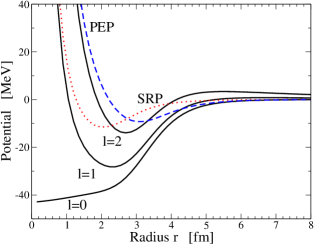
Figure 2: (color online) Radial part of the core-halo potentials $v_{0}^{l}$ (solid lines) for $l=0,$ $1$ and $2$ and the SUSY transformed $v_{1}^{l=0}$ (dashed line) and ${\underline{v}}_{1}^{l=0}$ (dotted line).

We work on a constant step mesh containing 400 points and ranging from 0 fm to 50 fm. We show in Fig. 12 the original potential $v_{0}^{l}$ for $l=0$, $l=1$ and $l=2$ (solid lines), the SRP $v_{1}^{l=0}$ (dashed line) and the PEP ${\underline{v}}_{1}^{l=0}$ (dotted line).

We can obtain analytical expressions near $r=0$ and for large $r$. Indeed, near zero, the lowest energy state behaves like $r^{l+1}$ and asymptotically, it behaves like $\exp(-\gamma_{0}r)$ with $\gamma_{0}=\sqrt{-2mE_{0}^{0l}}/\hbar$. These asymptotics and therefore the following expressions are very general for all potentials which are regular at the origin and vanish for large $r$. We find that the super-potentials behave like ($r\rightarrow 0$)

$$w_{0}^{l}(r) \stackrel{{\scriptstyle 0}}{{\sim}} \frac{l+1}{r}\hbox{ and }w_{0}^{l}(r)\stackrel{{\scriptstyle\infty}}{{\sim}}-\gamma_{0},$$ (43)

$$\underline{\underline{w}}_{0}^{l}(r) \stackrel{{\scriptstyle 0}}{{\sim}} \frac{2l+3}{r}\hbox{ and }\underline{\underline{w}}_{0}^{l}(r)\stackrel{{\scriptstyle\infty}}{{\sim}}0,$$ (44)

and the potentials are for $r\rightarrow 0$

$$v_{1}^{l}(r) \stackrel{{\scriptstyle 0}}{{\sim}} v_{0}^{l}(r)+\frac{\hbar^{2}}{m}\frac{l+1}{r^{2}}=v_{0}^{l+1}(r),$$ (45)

$${\underline{v}}_{1}^{l}(r) \stackrel{{\scriptstyle 0}}{{\sim}} v_{0}^{l}(r)+\frac{\hbar^{2}}{m}\frac{2l+3}{r^{2}}=v_{0}^{l+2}(r),$$ (46)

and for $r\rightarrow\infty$

$$v_{1}^{l}(r) \stackrel{{\scriptstyle\infty}}{{\sim}} v_{0}^{l}(r),$$ (47)

$${\underline{v}}_{1}^{l}(r) \stackrel{{\scriptstyle\infty}}{{\sim}} v_{0}^{l}(r).$$ (48)

The creation/annihilation operators become

$$\hat{a}_{0}^{\pm} \stackrel{{\scriptstyle\infty}}{{\sim}} \mp\frac{i\hat{p}}{\sqrt{2m}}-\gamma_{0},$$ (49)

$$\hat{\underline{a}}_{0}^{\pm} \stackrel{{\scriptstyle\infty}}{{\sim}} \mp\frac{i\hat{p}}{\sqrt{2m}}+\gamma_{0}.$$ (50)

Using these asymptotic expressions, one find the following properties of the mapping operators:

$$\langle r|\hat{\mathrm{u}}_{0}^{\pm}|r^{\prime}\rangle \stackrel{{\scriptstyle\infty}}{{\sim}} \langle r|\frac{\mp i\hat{p}/\sqrt{2m}-\gamma_{0}}{\sqrt{\hat{p}^{2}/2m+\gamma_{0}^{2}}}|r^{\prime}\rangle,$$ (51)

$$\langle r|\hat{\mathrm{\underline{u}}}_{0}^{\pm}|r^{\prime}\rangle \stackrel{{\scriptstyle\infty}}{{\sim}} \delta(r-r^{\prime}).$$ (52)

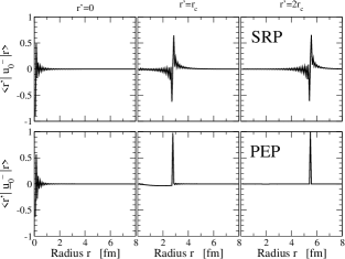
Figure 3: Matrix elements of $\mathrm{u}_{0}^{-}(r,r^{\prime})$ (top, SRP) and $\mathrm{\underline{u}}_{0}^{-}(r,r^{\prime})$ (bottom, PEP) for several values of $r^{\prime}$ ($r^{\prime}=0$, $r_{c}$, $2r_{c}$) calculated for the angular momentum $l=0$ inside the core-halo potential. We remind that $r_{c}$ is the radius of the ¹⁰Be core.

We present in Fig. 3 the matrix elements of $\langle r|\hat{\mathrm{u}}_{0}^{-}|r^{\prime}\rangle$ and $\langle r|\hat{\mathrm{\underline{u}}}_{0}^{-}|r^{\prime}\rangle$ as a function of $r$ for several values of $r^{\prime}$: $0,r_{c}$ and $2r_{c}$ where $r_{c}$ is the radius of the ¹⁰Be core. The peaks identifies the diagonal terms. We remark that the operator $\hat{\mathrm{u}}_{0}^{-}$ has important off-diagonal terms (for small and large values of $r^{\prime}$) while the operator $\hat{\mathrm{\underline{u}}}_{0}^{-}$ converges towards a delta function when $r^{\prime}$ increases. Hence, the restoration of the phase shift imposes $\hat{\mathrm{\underline{u}}}_{0}^{\pm}\sim\hat{1}$ for large values of $r^{\prime}$, however this relation breaks down close to the core where the off-diagonal terms become important.

V Electric excitation

In this section, we shall consider dynamical properties of nuclei within the consistent SUSY transformation we have developed in the previous sections and discuss how it may be approximated. We will discuss the modifications of the excitation operators, the doorway sensitivity, and finally, we will compute some transition elements and strength associated to monopole (E0), dipole (E1) and quadrupole (E2) electromagnetic excitations and the associated sum rules.

We assume that, prior to any SUSY transformation, the excitation operator takes the standard multipolar form

$$\hat{f}_{0}(\lambda,L,M)=\hat{f}_{0}^{\mathrm{rad}}(\lambda)\hat{Y}_{L,M},$$ (53)

with the radial excitation operator $\hat{f}_{0}^{\mathrm{rad}}(\lambda)=\hat{r}^{\lambda}$. We drop the coupling constant because we are only interested in the transformation of the radial excitation operator and the relative difference between the consistent SUSY transformation and its approximations. The E0 transition is induced by $\hat{f}_{0}(2,0,0)$ and the electromagnetic transitions E$\lambda$ are induced by $\hat{f}_{0}(\lambda,\lambda,M)$ ($\lambda\geq 1$). The SUSY transformation of the excitation operator is

$$\hat{f}_{k}(\lambda,L,M)=\hat{\mathrm{u}}_{k-1}^{+}\,\hat{f}_{0}(\lambda,L,M)\,\hat{\mathrm{u}}_{k-1}^{-}.$$

Introducing explicitly the angular momentum quantum numbers, the radial excitation operator is thus given by

$$\hat{f}_{k}^{l^{\prime}l}(\lambda)=\hat{\mathrm{u}}_{k-1}^{l^{\prime}+}\,\hat{f}_{0}^{\mathrm{rad}}(\lambda)\,\hat{\mathrm{u}}_{k-1}^{l-},$$ (54)

where $\hat{\mathrm{u}}_{k-1}^{l\,\pm}$ is the mapping operators $\hat{\mathrm{u}}_{k-1}^{\pm}$ in a subspace associated with the angular momentum $l$ (and $m$). The external operator $\hat{f}_{k}^{l^{\prime}l}(\lambda)$ allows transitions between different angular momentum space according to the selection rules deduced from the relation

$$\langle l^{\prime}m^{\prime}|\hat{f}_{k}(\lambda,L,M)|lm\rangle=\hat{f}_{k}^{l^{\prime}l}(\lambda)\langle l^{\prime}m^{\prime}|\hat{Y}_{L,M}|lm\rangle.$$ (55)

It should be noticed that, in Eq. 54 the mapping operator $\hat{\mathrm{u}}_{k-1}^{l\,\pm}$ on the right and on the left side of $\hat{f}_{0}^{\mathrm{rad}}(\lambda)$ may not correspond to the same angular momentum $l$. Moreover, while the original radial excitation operator $\hat{f}_{0}^{\mathrm{rad}}(\lambda)$ is diagonal (in the coordinate space), $\hat{f}_{k}^{l^{\prime}l}(\lambda)$ is no longer diagonal because the transformation operators $\hat{\mathrm{u}}_{k-1}^{l\,\pm}$ are non local.

V.1 Consistent excitation operator and its approximations

In the following, we shall perform the calculation of the excitation operator and some of the observables it induces. In the literature, the SUSY transformation is in general not applied to the excitation operator. Hence, instead of calculating the matrix elements induced by the consistent excitation operator $\hat{f}_{k}^{l^{\prime}l}(\lambda)$, the authors have evaluated the matrix elements of $\hat{f}_{0}^{\mathrm{rad}}(\lambda)$ with the SUSY transformed wave functions. We will refer to this approximation as the internal approximation. We introduce a second approximation called the diagonal approximation which consists simply of neglecting the off-diagonal terms in coordinate space of the consistent excitation operator.

As a first example we will study the $E0$ excitation of the halo neutron in the $s$-subspace. In this subspace the core blocks one orbital (1s) so that we have to perform a SRP or a PEP transformation to remove this occupied state from the halo Hilbert space and restore the phase shift. Of course, to be complete we have also to remove the occupied $p$-state but since the SUSY transformation is block-diagonal for the angular momentum quantum numbers this does not modify the dynamics in the $s$-subspace.

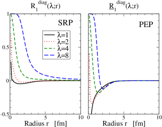
Figure 4: (color online) The normalized difference of diagonal matrix elements ($R_{k}^{\mathrm{diag}}(\lambda;r)$ for SRP transformation and ${\underline{R}}_{k}^{\mathrm{diag}}(\lambda;r)$ for PEP one) are represented for several values of $\lambda$ (1,2,4,8) for the electric excitation $E\lambda$ inside the s-space.

In order to evaluate the difference between the consistent SUSY transformation and its approximations, we define two quantities

$$R_{k}^{\mathrm{diag}}(\lambda;r) = \frac{\langle r|\Delta\hat{f}_{k}^{00}(\lambda)|r\rangle}{\langle r|\hat{f}_{k}^{00}(\lambda)|r\rangle},$$ (56)

$$R_{k}^{\mathrm{off}}(\lambda;r,r^{\prime}) = \frac{\langle r|\hat{f}_{k}^{00}(\lambda)|r^{\prime}\rangle}{\langle r|\hat{f}_{k}^{00}(\lambda)|r\rangle},$$ (57)

where

$$\Delta\hat{f}_{k}^{l^{\prime}l}(\lambda)=\hat{f}_{k}^{l^{\prime}l}(\lambda)-\hat{f}_{0}^{\mathrm{rad}}(\lambda)$$

is the difference between the excitation operator consistently transformed $\hat{f}_{k}^{l^{\prime}l}(\lambda)$ and the original excitation operator $\hat{f}_{0}^{\mathrm{rad}}(\lambda)$. The ratio $R_{k}^{\mathrm{diag}}(\lambda;r)$ evaluates the difference between the diagonal part of the consistent excitation operator and the original operator, normalized to the value of the diagonal part of the consistent operator. It gives an evaluation of the approximation for the diagonal part of the excitation operator. Fig. 4 shows the ratio $R_{k}^{\mathrm{diag}}(\lambda;r)$ and $\underline{R}_{k}^{\mathrm{diag}}(\lambda;r)$ for $\lambda$=1, 2, 4, 8 in the case of the 1s SRP and PEP transformation respectively. We remark that for large radii $r$, the diagonal part of the excitation operator is close to the original one ($R_{k}^{\mathrm{diag}}(\lambda;r)\sim 0$). This is a consequence of the asymptotic properties of the mapping operator as it has been discussed in the section IV.2. For small radii $r$, the diagonal part of the excitation operator is strongly modified, the ratio $R_{k}^{\mathrm{diag}}(\lambda;r)\sim 1$ revealing that $\langle r|\hat{f}_{k}^{\mathrm{rad}}|r\rangle\gg\langle r|\hat{f}_{0}^{\mathrm{rad}}|r\rangle$. This difference persists through a large range of radial coordinates. This range increases with $\lambda$, it is wider for SRP transformation compared with PEP transformations.

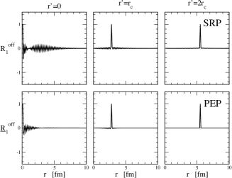
Figure 5: The normalized off-diagonal matrix elements ($R_{k}^{\mathrm{off}}(\lambda=4;r,r^{\prime})$ and ${\underline{R}}_{k}^{\mathrm{off}}(\lambda=4;r,r^{\prime})$) are represented as a function of $r$ for several values of r’ (0, $r_{c}$, $2r_{c}$) for the electric excitation $E\lambda$ inside the s-space.

On the other hand, the ratio $R_{k}^{\mathrm{off}}(\lambda;r,r^{\prime})$ evaluates the amplitude of the off-diagonal terms in coordinate space normalized to the diagonal term of the consistent excitation operator. In Fig. 5, we represent the ratio $R_{k}^{\mathrm{off}}(\lambda=4;r,r^{\prime})$ and $\underline{R}_{k}^{\mathrm{off}}(\lambda=4;r,r^{\prime})$ for the SRP and PEP transformation respectively, and for three values of $r^{\prime}$: 0, $r_{c}$ and $2r_{c}$. For SRP transformation, off diagonal terms are important for small $r^{\prime}$ and decrease in relative magnitude while $r^{\prime}$ increases. Off-diagonal terms are non zero in a wide range and we will show in the next paragraphs that they can have a more important effect on observables than the diagonal terms. For the PEP transformation the off diagonal terms are smaller and become negligible for intermediate and large $r^{\prime}$ ($\geq r_{c}$) as required by the restoration of the asymptotic behavior.

In all the cases presented here, the consistent excitation operator is different from the original one in the space region inside the core potential. Hence, from this observation, we can expect that there will be important effects induced by the consistent calculation if and only if the calculated observable is sensitive to the space region inside the core potential.

V.2 Transformation of the doorway state

We want now to evaluate both contributions of the diagonal and off-diagonal excitation operators on the matrix elements. For that, we introduce the doorway state defined as

$$|\delta\varphi_{k}(\lambda,l\rightarrow l^{\prime})\rangle=\hat{f}_{k}^{l^{\prime}l}(\lambda)|\varphi_{k}^{l}\rangle.$$

In the following, we have chosen for $|\varphi_{k}^{l}\rangle$ the ground state of $\hat{h}_{k}^{l}$.

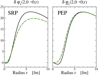
Figure 6: (color online) The doorway state $\delta\varphi_{1}(\lambda=2,0\rightarrow 0;r)$ and $\delta\underline{\varphi}_{1}(\lambda=2,0\rightarrow 0;r)$ of electric excitations for SRP and PEP transformations respectively. The solid line stands for the consistent excitation operator, dotted line for the internal approximation and dashed line for the diagonal approximation.

We represent in Fig. 6 the doorway state $\delta\varphi_{1}(\lambda=2,0\rightarrow 0;r)$ and $\delta\underline{\varphi}_{1}(\lambda=2,0\rightarrow 0;r)$ for the SRP and PEP transformations respectively. The solid line stands for the consistent excitation operator, dotted line for the internal approximation and dashed line for the diagonal approximation. We remark that the internal approximation and the diagonal approximation are indistinguishable. This shows that off-diagonal terms are the most important sources of modification of the excitation operator.

Moreover, the consistent doorway state changes sign while the two approximations remains positive. This affects the node structure of the wave function and may induce strong modifications for forbidden transition as we will see in the next paragraph.

V.3 Single particle reduced transition probability

The single-particle reduced transition probabilities are defined as Bor69

$$B_{k}(E0,i\rightarrow f)=\langle\varphi_{k}^{f}|\hat{f}_{k}^{l_{f}\,l_{i}}(2)|\varphi_{k}^{i}\rangle$$ (58)

with $l_{f}=l_{i}$ and as

$$B_{k}(E\lambda,i\rightarrow f) = \langle\varphi_{k}^{f}|\hat{f}_{k}^{l_{f}\,l_{i}}(\lambda)|\varphi_{k}^{i}\rangle$$ (59)

with $\left|l_{i}-\lambda\right|\leq l_{f}\leq l_{i}+\lambda$ and for $\lambda\geq 1$. In order to simplify the notations, the states $i$ and $j$ are labeled according to the original space prior to any transformation. In the halo case, developed above, all the final states are in the continuum so it will not be possible to use directly these definitions. In the next section we will introduce the strength function, a more general way to look at transition probabilities which is suitable for the case of excitation towards continuum and which can thus be used in the halo case. To get results for the transition probabilities between discreet states, in the present section, we will restrict the discussion to the harmonic oscillator model (see section IV.1). To simplify the discussion, we will consider that the nucleons of the core only occupy the $1s$ orbital and we will study the excitation of an additional neutron in the $2s$ orbital. We have computed numerically the reduced matrix elements ${\underline{B}}_{1}$(E0) and ${\underline{B}}_{1}$(E1) for the PEP transformation. The results are presented respectively in the tables 1 and 2. In the harmonic oscillator, due to selection rules, from the 2s the monopole operator $\hat{r}^{2}$ can induce transition only towards the 3s. In table 1, the first line shows the result of the matrix elements ($B$) induced by the consistent excitation operator. As expected, the forbidden transition are zero within the numerical uncertainty indicated in parenthesis.

The matrix elements, $\widetilde{B}$, induced by the internal excitation operator are showed in the second line of table 1. For allowed transitions, the internal approximation modifies by about 20% the exact matrix element, but the main effect of this approximation is that it induces forbidden transitions from 2s to 4s-7s states.

On the other hand, in the case of E1 electromagnetic transition, the selection rules of dipole transitions in the harmonic oscillator allow transition from 2s states to 1p and 2p states. The same phenomenon is observed in table 1 and table 2: the internal approximation produces spurious excitation of forbidden states. Moreover, for the allowed transition the error goes up to more then a factor $2$.

f	3s	4s	5s	6s	7s
${\underline{B}}_{1}$(E0)	1.1$\times$104	o(10-4)	o(10-8)	o(10-7)	o(10-7)
$\widetilde{{\underline{B}}}_{1}$(E0)	9.2$\times$103	1.5$\times$101	1.3	7.1$\times$10-2	1.4$\times$10-4

Table 1: ${\underline{B}}_{1}$(E0, 2s$\rightarrow$ f) for the PEP transformed harmonic oscillator potential. $\widetilde{\underline{B}}_{1}$(E0, 2s$\rightarrow$ f) is the matrix element induced by the internal approximation of the excitation operator.

f	1p	2p	3p	4p	5p
${\underline{B}}_{1}$(E1)	5.0$\times$102	1.2$\times$103	o(10-6)	o(10-7)	o(10-6)
$\widetilde{{\underline{B}}}_{1}$(E1)	1.2$\times$103	8.0$\times$102	9.5	1.2	7.8$\times$10-2

Table 2: $\underline{B}_{1}$(E1, 2s$\rightarrow$ f) for the PEP transformed harmonic oscillator potential. $\widetilde{\underline{B}}_{1}$(E1, 2s$\rightarrow$ f) is the matrix element induced by the internal approximation of the excitation operator.

V.4 Strength

The very important discrepancy between the internal and the complete SUSY observed in the case of the harmonic oscillator might be a peculiarity due to the symmetry of this model. Let us thus come back to the physical case of the ¹¹Be halo nuclei for which transitions between orbitals belonging to the same l-space are all allowed. Now we should remove the $1s$ (-25 MeV) and $1p$ (-12 MeV) orbitals occupied by the core neutrons so that only one bound state ($2s$) is available for the halo neutron. The excitations can only promote the halo neutron to the continuum. Hereafter, the eigenstates and the continuum states will be obtained from the diagonalization of the Hamiltonian inside a box going up to 50 fm with 400 points.

In order to discuss transition towards the continuum, we introduce the strength:

$$S_{k}(\mathrm{E}\lambda,i,\omega) = \sum_{f}|B_{k}(\mathrm{E}\lambda,i\rightarrow f)|^{2}\delta(\omega-E_{f}+E_{i}),$$

where $i$ is the initial state, here the $2s$ orbital, and the final states $f$ are the continuum states of the box. The single particle energies are $E_{i}$ and $E_{f}$ respectively. Since we perform the calculation in a box the continuum is discreetized. In order to obtain a smooth strength function one often smoothes the obtained results with a Gaussian or a Lorentzian function. In this paper we will do both.

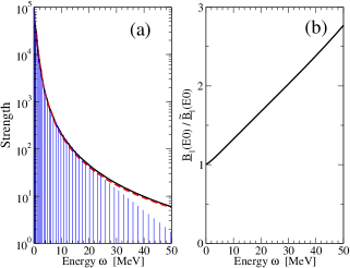
Figure 7: (color online) For monopole excitation: Left (a) the bars are the reduced transition probabilities ${\underline{B}}_{1}$(E0) for the continuum states discreetized in the considered box, the solid line is the strength function resulting from a Lorentzian smoothing ($\Gamma$=500 keV) and the dashed line is the result of the internal approximation. In part (b), we show the ratio ${\underline{B}}_{1}$(E0)/$\widetilde{\underline{B}}_{1}$(E0).

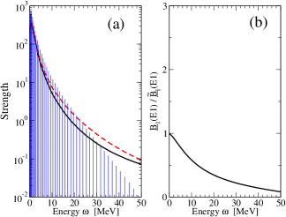
Figure 8: (color online) Same as Fig. 7 for dipole transitions.

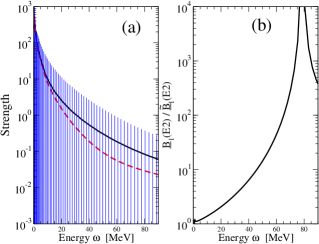
Figure 9: (color online) Same as Fig. 7 for quadrupole transitions.

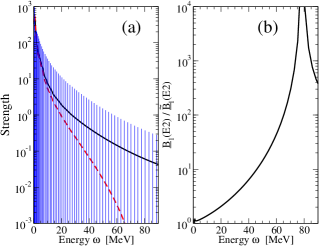
Figure 10: (color online) Same as Fig. 9 with Gaussian smoothing.

Strengths for PEP transformations for E0, E1 and E2 transitions are presented in the parts (a) of Fig. 7-8-9 with a Lorentzian smoothing ($\Gamma=500$ keV) and Fig. 10 with a Gaussian smoothing. The part (b) of each figure gives directly the ratio ${\underline{B}}_{1}$(E$\lambda$ )/$\widetilde{\underline{B}}_{1}$(E$\lambda$ ) computed for individual states.

For the monopole mode, using a Lorentzian smoothing the consistent strength and the internal strength appears to be very similar (see Fig. 7-a) even if the ratio ${\underline{B}}_{1}$(E0)/$\widetilde{\underline{B}}_{1}$(E0) computed for individual states (see part (b) of the figure) is very different from $1$ for large values of the final excitation energy $E_{f}$.

The dipole excitations connect the states of two different l-subspace. On the smoothed ${\underline{S}}_{1}$(E1) strength (see Fig. 8-a) we only observe a small over estimation of the strength for large values of $E_{f}$ but again the effect seems much larger on the ratio ${\underline{B}}_{1}$(E1)/$\widetilde{\underline{B}}_{1}$(E1). In Fig. 9, we represent the strength ${\underline{S}}_{1}$(E2). In the l=2 subspace, there are no core states and consequently, the SUSY transformation is in fact the unity. The smoothed strength appears to be only slightly under-estimated by the internal approximation again in contradiction with the ratio ${\underline{B}}_{1}$(E2)/$\widetilde{\underline{B}}_{1}$(E2) which exhibits a strong discrepancy.

In order to solve the contradiction we have first studied the role of the smoothing. We have found that the situation is different with a Gaussian smoothing as illustrated in Fig. 10. This difference is due to the difference in the tails of the two smoothing functions: the long tails of the Lorentzian function associated with the low energy states which have a large ${\underline{B}}_{1}$(E0) dominate even at large energy when a Lorentzian form factor is used. Indeed, since the difference between the two calculations is small for these dominating states the final Lorentzian-smoothed strengths for the two calculations are rather close in contradiction with the direct ratio of individual excitation probabilities or the results of the Gaussian smoothing.

To avoid the ambiguity of the smoothing method we have studied the continuum limit by a direct scaling of the numerical box size (we have also tested the role of the mesh size). We have observed that the ratio ${\underline{B}}_{1}$/$\widetilde{\underline{B}}_{1}$ computed for each individual state does not change shape going to the continuum limit while the smoothed strengths vary and exhibit a strong dependence into the smoothing functional and parameters. Therefore, the ratio ${\underline{B}}_{1}$(E0)/$\widetilde{\underline{B}}_{1}$(E0) provides in fact the correct continuum limit and the large observed discrepancy at high energy between the internal and the complete SUSY transformation is the physical one. This is even better illustrated by considering integrated effects like effects on the sum rules.

V.5 Sum rules

By integrating the strength over the energy, we can define different sum rules $m_{t}$

$$m_{t}(E\lambda)\equiv\int\!\!\!d\omega\,\,\omega^{t}S(E\lambda,i=0,\omega),$$ (61)

where $t$ is the weight of the energy. In the frozen core approximation, the sum rules $m_{0}$ and $m_{1}$ can be obtained from the halo wave function according to

$$m_{0} = \langle\Phi_{\mathrm{v}}|\hat{f}_{0}\hat{P}_{\mathrm{v}}\hat{f}_{0}|\Phi_{\mathrm{v}}\rangle-\left(\langle\Phi_{\mathrm{v}}|\hat{f}_{0}|\Phi_{\mathrm{v}}\rangle\right)^{2},$$ (62)

$$m_{1} = \frac{1}{2}\langle\Phi_{\mathrm{v}}|[\hat{f}_{0}\hat{P}_{\mathrm{v}},[\hat{h}_{0}^{l}\hat{P}_{\mathrm{v}},\hat{f}_{0}\hat{P}_{\mathrm{v}}]]|\Phi_{\mathrm{v}}\rangle.$$ (63)

where $\hat{f}_{0}$ is the excitation operator defined by Eq. 53. We define the internal approximation for the sum rule as $\widetilde{m}_{t}$ for which the projector $P_{\mathrm{v}}$ have been removed. The Pauli principle is no longer respected. In order to estimate the error induced in the calculation of $\widetilde{m}_{t}$ compared to $m_{t}$, we have estimated the ratios $(m_{t}-\widetilde{m}_{t})/m_{t}$ and we have found the results presented in Table 3. The relative error induced by the internal approximation increases with the weight. This result is compatible with the results presented in Fig. 7 and Fig. 8: when the weight increases, the contribution of large energy increases and the discrepancies between the consistent SUSY and its internal approximation increase also.

	$(\underline{m}_{0}-\widetilde{pep{m}}_{0})/\underline{m}_{0}$	$(\underline{m}_{1}-\widetilde{\underline{m}}_{1})/\underline{m}_{1}$	$({\underline{m}}_{2}-\widetilde{\underline{m}}_{2})/{\underline{m}}_{2}$
$E0$	1.4%	3.9%	17.4%
$E1$	-6.8%	-33.3%	-93.1%

Table 3: This table presents the relative error induced in the calculation of the energy weighted sum rules by the internal approximation of PEP transformations.

VI Response to a Gaussian excitation

In the previous section, we have shown that the PEP transformation modifies essentially the external excitation operator in the space region located inside the core potential. The electric operators $\hat{r}^{\lambda}\hat{Y}_{LM}$ studied in the previous section which can be seen as a multiple expansion of a Coulomb field far from the nucleus or as the low momentum transfer limit of a plane wave scattering are strong far from the nucleus. Hence, the effect of the PEP transformation on the excitation process has been found to not be too large. However, this is not always the case and in particular nuclear scattering and/or large momentum transfer reaction correspond to much shorter distances. In order to study the effect of the PEP transformation on such kind of scattering, in this section, we study the response to a Gaussian excitation which can strongly overlap with the core potential. Gaussian potential can be induced by an external nuclear potential as well as a residual two-body interaction between particle in the halo. In a similar spirit of the previous section, we will not study a specific process but the response to a one body Gaussian potential centered around $\mathbf{r}_{0}$ defined as

$$g_{0}(\mathbf{r})=-\frac{g_{0}}{\left(\sqrt{\pi}\mu\right)^{3}}\exp\left(-\frac{(\mathbf{r}-\mathbf{r}_{0})^{2}}{\mu^{2}}\right),$$

where the norm of the interaction is $g_{0}$=450 MeV.fm³ and its range is $\mu$=2 fm. The SUSY transformation of this potential is

$$\hat{g}_{k}^{l^{\prime}l}=\hat{\mathrm{u}}_{k-1}^{l^{\prime}\,-}\,\hat{g}_{0}\,\hat{\mathrm{u}}_{k-1}^{l\,+}.$$

Similarly to the previous section, we define two quantities that measure the modification of the SUSY transformation on the diagonal and off-diagonal terms of the Gaussian potential:

$$Q_{k}^{\mathrm{diag}}(r) = \frac{\langle r|\hat{g}_{k}^{00}-\hat{g}_{0}^{00}|r\rangle}{\langle r|\hat{g}_{k}|r\rangle},$$ (64)

$$Q_{k}^{\mathrm{off}}(r,r^{\prime}) = \frac{\langle r|\hat{g}_{k}^{00}|r^{\prime}\rangle}{\langle r|\hat{g}_{k}^{00}|r\rangle}.$$ (65)

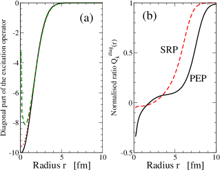
Figure 11: (color online) Left (a) the initial Gaussian potential($l=0$) (solid line), SRP (dotted line) and PEP (dashed line) potentials. In part(b), we show the ratio $Q_{1}^{\mathrm{diag}}(r)$ for SRP (dashed) and PEP (dotted) potentials.

In Fig. 11, we fix $r_{0}=0$ and we represent (a) the diagonal part of $g_{1}$ (dotted line) and ${\underline{g}}_{1}$ (dashed line) compared to the original potential $g_{0}$ (solid line), and (b) the ratio $Q_{k}^{\mathrm{diag}}(r)$ for the SRP transformation (dashed line) and PEP transformation (solid line). In the very central region, the PEP transformations modify the potential by a factor 30%. At large distance $r$, because of the Gaussian shape centered on zero of $g_{0}(r^{\prime})$, an important relative weight is given to small radii in the summation $\langle r|\hat{g}_{k}|r\rangle=\int dr^{\prime}\langle r|\mathrm{\hat{u}}^{-}|r^{\prime}\rangle g_{0}(r^{\prime})\langle r^{\prime}|\mathrm{\hat{u}}|r\rangle$. The result of this effect is that the range of $\langle r|\hat{g}_{k}|r\rangle$ is slightly increased compared to $g_{0}(r^{\prime})$ and because of the exponential behavior of the excitation operator this is enough to make the ratio $Q_{k}^{\mathrm{diag}}(r)\sim 1$.

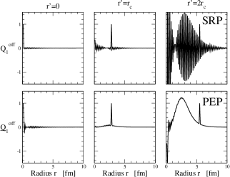
Figure 12: The ratios $Q_{1}^{\mathrm{off}}(r,r^{\prime})$ in the $l=0$ channel as a function of $r$ for several values of $r^{\prime}$ ($0$, $r_{c}$ and $2r_{c}$) in the case of a Gaussian potential.

In Fig. 12, we show the ratio $Q_{1}^{\mathrm{off}}(r,r^{\prime})$ for the SRP transformation (upper panel) and the PEP transformation (lower panel) and for three different values of $r^{\prime}$: 0, $r_{c}$ and $2r_{c}$. For values of $r^{\prime}$ inside the potential, off-diagonal terms are small compared to the diagonal term but they are spread over a large range of coordinates, and their integrated effect can counter balance their small values. Outside the potential, the off-diagonal terms become very important and even larger than the diagonal term for both SRP and PEP transformations.

Both diagonal and off-diagonal terms have an effect on the particle wave function that can be estimated with the doorway state

$$|\delta\varphi_{k}(l\rightarrow l^{\prime})\rangle=\hat{g}_{k}^{l^{\prime}l}|\varphi_{k}^{l}\rangle.$$

In the following, we have chosen for $|\varphi_{k}^{l}\rangle$ the ground state of $\hat{h}_{k}^{l}$.

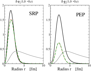
Figure 13: (color online) The doorway state in the $l=0$ channel $\delta\varphi_{1}(0\rightarrow 0;r)$ produced by a Gaussian excitation for SRP and PEP transformations. The solid line stands for the consistent excitation operator, dotted line for the internal approximation and dashed line for the diagonal approximation. The thin line stands for the initial wave function $\varphi_{1}^{0}(r)$.

In Fig. 13, we represent $\delta\varphi_{1}(0\rightarrow 0;r)$ for SRP and PEP transformations. The solid line stands for the consistent transformation of the Gaussian interaction, the dotted line for its internal approximation and the dashed line for the diagonal approximation. The internal approximation and the diagonal approximation give about the same results but are both very different from the consistent calculation. These two figures illustrate the importance of the off-diagonal terms which induce very different doorway states.

Summarizing our results, we can assert that the Gaussian interaction is considerably modified by the SUSY transformations and the internal approximation is certainly a bad approximation as it is illustrated in Fig. 13. Hence, calculations of structure properties and reaction mechanism which involve SUSY transformations should never neglect the transformation of the excitation operator (or residual interaction) for radii inside the core potential.

VII Conclusion

In this article, we discussed a consistent framework to perform quantum mechanics SUSY transformation to take into account the internal degrees of freedom in a core approximation. This method is totally equivalent to the full projector-method and is formally very interesting since it provides justifications for effective core-nucleon interactions and nucleon-nucleon residual interaction. In this study, we have considered several kinds of external fields and performed a consistent SUSY transformation. The consistent SUSY transformation provides equivalent effective interactions between composite particle systems and thus can be safely used to describe nuclear structure and reaction of nuclei. The consistent transformation of additional fields as well as the transformation of the wave functions (or the observables) is usually neglected in the literature (internal approximation)and we have shown that it is not always justified.

Our conclusions are the following: in the case of electromagnetic induced transitions, consistent SUSY transformation conserves all selection rules while the internal approximation violates it. Performing different comparisons we have shown that the discrepancies might be large, affecting the node structure of the doorway states and changing the transition probabilities by sizeable factors. Even the sum rules can be affected by a large percentage, e.g. 33% for the energy weighted sum rule of the dipole excitation. Hence, the use of the internal approximation for external excitation operator might be dangerous and the results obtained should be carefully discussed. But the main discrepancies between the consistent calculation and its internal approximation appear for external fields which have a strong overlap with the core potential. For instance, it is the case of the Gaussian interaction centered at small distance ($r_{0}<r_{c}$).

In all the cases, we have shown that due to the SUSY transformation, the off-diagonal terms of the external fields are often more important than the diagonal ones. This forbids an approximation which would be to take into account only the SUSY modification of the diagonal term. Hence, the SUSY transformation has to be fully implemented in order to preserve the symmetry of the original Hamiltonian.

All the discussion related to the excitation operator is valid for the observables. Since the wave functions are transformed either they should be transformed back before evaluating average values or the observables should be also transformed before being applied on a transformed state.

In conclusion, in this article, we have stressed the importance to keep the consistency of the QM-SUSY framework if there is an overlap between the core potential and the additional interactions (excitation operator or observables). For instance, in a recent article Hesse et al. Hes99 have performed the internal SUSY approximation and they have shown that in order to reproduce the known binding energies and radii of ⁶He, ¹¹Li and ¹¹Be halo nuclei, a readjustment of the core-neutron interaction is required. This effect might be induced by the internal SUSY approximation which treats improperly the $r^{2}$ observable for the halo neutrons and the residual interaction between them. The consistent SUSY framework would be a way to extract informations concerning the neutron-neutron interaction in the halo because there is a unique mapping between the original known interaction and the effective one which includes consistent removal of core orbits.

- (1) E. Witten, Nucl. Phys. B 188 (1981) 513.
- (2) A.A. Andrianov, N.V. Borisov & M.V. Ioffe, Phys. Lett. 105 A (1984) 19.
- (3) C.V. Sukumar, J. Phys. A 18 (1985) 2917.
- (4) D. Baye, Phys. Rev. Lett. 58 (1987) 2738.
- (5) F. Cooper, A. Khare & U. Sukhatme, Phys. Rep. 251 (1995) 277.
- (6) D. Ridikas et al., Nucl. Phys. A 609 (1996) 21.
- (7) P. Capel et al., Phys. Lett. B 552 (2003) 145.
- (8) B. Gönül et al., Eur. Phys. J. A 9 (2000) 19.
- (9) M. Hesse et al., Phys. Lett. B 455 (1999) 1.
- (10) I.J. Thompson et al., Phys. Rev. C 61 (2000) 24318.
- (11) F. Cannata and M. Ioffe, J. Phys. A: Math. Gen. 34 (2001) 1129.
- (12) P. Descouvemont, C. Daniel & D. Baye, Phys. Rev. C 67 (2003) 44309.
- (13) H. Leeb et al., Phys. Rev. C 62 (2000) 64003.
- (14) A.M. Shirokov and V.N. Sidorenko, Phys. Atom. Nucl. 63 (2000) 1993-1998; Yad. Fiz. 63 (2000) 2085-2090.
- (15) B.F. Samsonov and Fl. Stancu, Phys. Rev. C 67 (2003) 054005.
- (16) K. Chadan and P.C. Sabatier, Inverse Problems in Quantum Scattering Theory, 1977 (Berlin, Springer).
- (17) D. Baye, J. Phys. A: Math. Gen. 20 (1987) 5529.
- (18) L.U. Ancarani and D. Baye, Phys. Rev. A 46 (1992) 206.
- (19) R.D. Lawson, Theory of the nuclear shell model, Clarendon Press Oxford (1980).
- (20) I. Tanihata et al. Phys. Rev. Lett. 55 (1985) 2676.
- (21) S. Grévy, O. Sorlin and N. Vinh Mau, Phys. Rev. C 56 (1997) 2885.
- (22) A. Bohr and B. Mottelson, Volume 1-2, Nuclear Structure (Benjamin, Reading, 1969).