Boundary Conditions of the Hydro-Cascade Model and Relativistic Kinetic Equations for Finite Domains

Abstract

A detailed analysis of the coupled relativistic kinetic equations for two domains separated by a hypersurface having both space- and time-like parts is presented. Integrating the derived set of transport equations, we obtain the correct system of the hydro+cascade equations to model the relativistic nuclear collision process. Remarkably, the conservation laws on the boundary between domains conserve separately both the incoming and outgoing components of energy, momentum and baryonic charge. Thus, the relativistic kinetic theory generates twice the number of conservation laws compared to traditional hydrodynamics. Our analysis shows that these boundary conditions between domains, the three flux discontinuity, can be satisfied only by a special superposition of two cut-off distribution functions for the “out” domain. All these results are applied to the case of the phase transition between quark gluon plasma and hadronic matter. The possible consequences for an improved hydro+cascade description of the relativistic nuclear collisions are discussed. The unique properties of the three flux discontinuity and their effect on the space-time evolution of the transverse expansion are also analyzed. The possible modifications of both transversal radii from pion correlations generated by a correct hydro+cascade approach are discussed.

PACS numbers: 25.75.Ld

Key words: kinetic equations with source terms, hydro+cascade equations, conservation laws, three flux discontinuity

I Introduction

The modern history of relativistic hydrodynamics started more than fifty years ago when L. D. Landau suggested [1] its use to describe the expansion of the strongly interacting matter that is formed in high energy hadronic collisions. Since that time there arose a fundamental problem of relativistic hydrodynamics known as the freeze-out problem. In other words, one has to know how to stop solving the hydrodynamical equations and convert the matter into free streaming particles. There were several ways suggested to handle it, but only recently a new approach to solve the freeze-out problem in relativistic hydrodynamics has been invented by Bass and Dumitru (BD model) [2] and further developed by Teaney, Lauret and Shuryak (TLS model) [3]. These hydro + cascade models assume that the nucleus-nucleus collisions proceed in three stages: hydrodynamic expansion (hydro) of the quark gluon plasma (QGP), phase transition from the QGP to the hadron gas (HG) and the stage of hadronic rescattering and resonance decays (cascade). The switch from hydro to cascade modeling takes place at the boundary between the mixed and hadronic phases. The spectrum of hadrons leaving this hypersurface of the QGP–HG transition is taken as input for the cascade.

This approach incorporates the best features of both the hydrodynamical and cascade descriptions. It allows for, on one hand, the calculation of the phase transition between the quark gluon plasma and hadron gas using hydrodynamics and, on the other hand, the freeze-out of hadron spectra using the cascade description. This approach allows one to overcome the usual difficulty of transport models in modeling phase transition phenomenon. For this reason, this approach has been rather successful in explaining a variety of collective phenomena that has been observed at the CERN Super Proton Collider (SPS) and Brookhaven Relativistic Heavy Ion Collider (RHIC) energies. However, both the BD and TLS models face some fundamental difficulties which cannot be ignored (see a detailed discussion in [4]). Thus, within the BD approach the initial distribution for the cascade is found using the Cooper-Frye  formula [5], which takes into account particles with all possible velocities, whereas in the TLS model the initial cascade distribution is given by the cut-off  formula [6, 7], which accounts for only those particles that can leave the phase boundary. As shown in Ref. [4] the Cooper-Frye  formula leads to causal and mathematical problems in the present version of the BD model because the QGP–HG phase boundary inevitably has time-like parts. On the other hand, the TLS model does not conserve energy, momentum and number of charges and this, as will be demonstrated later, is due to the fact that the equations of motion used in [3] are incomplete and, hence, should be modified.

These difficulties are likely in part responsible for the fact that the existing hydro+cascade models, like the more simplified ones, fail to explain the HBT puzzle [8], i.e. the fact that the experimental HBT radii at RHIC are very similar to those found at SPS, even though the centre of mass energy is larger by an order of magnitude. Therefore, it turns out that the hydro+cascade approach successfully parameterizes the one-particle momentum spectra and their moments, but does not describe the space-time picture of the nuclear collision as probed by two-particle interferometry.

The main difficulty of the hydro + cascade approach looks similar to the traditional problem of freeze-out in relativistic hydrodynamics [6, 7]. In both cases the domains (subsystems) have time-like boundaries through which the exchange of particles occurs and this fact should be taken into account. In relativistic hydrodynamics this problem was solved by the constraints which appear on the freeze-out hypersurface and provide the global energy-momentum and charge conservation [6, 7, 9]. A generalization of the usual Boltzmann equation which accounts for the exchange of particles on the time-like boundary between domains in the relativistic kinetic theory was given recently in Ref. [4]. It was shown that the kinetic equations describing the exchange of particles on the time-like boundary between subsystems should necessarily contain the $\delta$-like source terms. From these kinetic equations the correct system of hydro+cascade equations to model the relativistic nuclear collision process was derived without specifying the properties of the separating hypersurface. However, both an explicit switch off criterion from the hydro equation to the cascade one and the boundary conditions between them were not considered in [4]. The present work is devoted to the analysis of the boundary conditions for the system of hydro+cascade equations. This is necessary to formulate the numerical algorithm for solving the hydro+cascade equations.

The paper is organized as follows. In Sect. 2 a brief derivation of the set of kinetic equations is given and source terms are obtained. In Sect. 3 the analog of the collision integrals is discussed and a fully covariant formulation of the system of coupled kinetic equations is found. The relation between the system obtained and the relativistic Boltzmann equation is also considered. The correct equations of motion for the hydro + cascade approach and their boundary conditions are analyzed in Sect. 4. There it is also shown that the existence of strong discontinuities across the space-like boundary, the time-like shocks, is in contradiction with the basic assumptions of a transport approach. The solutions of boundary conditions between the hydro and cascade domains for a single degree of freedom and for many degrees of freedom are discussed in Sect. 5 and 6, respectively. The conclusions are given in Sect. 7.

II Drift Term for Semi-Infinite Domain

Let us consider two semi-infinite domains, “in” and “out”, separated by the hypersurface $\Sigma^{*}$ which, for the purpose of presenting the idea, we assume to be given in (3+1) dimensions by a single valued function $t=t^{*}(\bar{x})=x_{0}^{*}(\bar{x})$. The latter is assumed to be a unique solution of the equation ${\cal F}^{*}(t,\bar{x})=0$ (a switch off criterion) which has a positive time derivative $\partial_{0}{\cal F}^{*}(t^{*},\bar{x})>0$ on the hypersurface $\Sigma^{*}$. The distribution function $\phi_{in}(x,p)$ for $t\leq t^{*}(\bar{x})$ is assumed to belong to the “in” domain, whereas $\phi_{out}(x,p)$ denotes the distribution function of the “out” domain for $t\geq t^{*}(\bar{x})$(see Fig.1). In this work it is assumed that the initial conditions for $\phi_{in}(x,p)$ are given, whereas on $\Sigma^{*}$ the function $\phi_{out}(x,p)$ is allowed to differ from $\phi_{in}(x,p)$ and this will modify the kinetic equations for both functions. For simplicity we consider a classical gas of point-like Boltzmann particles.

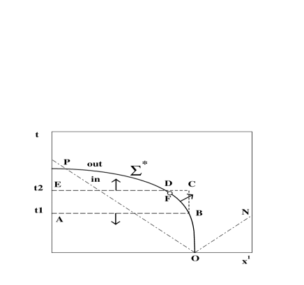
FIG. 1.: Schematic two dimensional picture of the boundary hypersurface $\Sigma^{*}$ (solid curve). Arrows show the external normal vectors. The light cone $NOP$ is shown by the dash-dotted line. The point $F$ divides $\Sigma^{*}$ into the time-like ($OF$) and space-like ($FP$) parts.

Similar to Ref. [10] we derive the kinetic equations for $\phi_{in}(x,p)$ and $\phi_{out}(x,p)$ from the requirement of particle number conservation. Therefore, the particles leaving one domain and crossing the hypersurface $\Sigma^{*}$ should be subtracted from the corresponding distribution function and added to the other. Now consider the closed hypersurface of the “in” domain, $\Delta x^{3}$ (shown as the contour $ABDE$ in Fig.1), which consists of two semi-planes $\sigma_{t1}$ and $\sigma_{t2}$ of constant time $t1$ and $t2$, respectively, that are connected from $t1$ to $t2>t1$ by the arc $BD$ of the boundary $\Sigma^{*}(t1,t2)$ in Fig.1. The original number of particles on the hypersurface $\sigma_{t1}$ is given by the standard expression [10]

$$N_{1}=-\int\limits_{\sigma_{t1}}d\Sigma_{\mu}\frac{d^{3}p}{p^{0}}~{}p^{\mu}~{}\phi_{in}(x,p)\,,$$ (1)

where $d\Sigma_{\mu}$ is the external normal vector to $\sigma_{t1}$ and, hence, the product $p^{\mu}d\Sigma_{\mu}\leq 0$ is non-positive. It is clear that these particles can cross either hypersurface $\sigma_{t2}$ or $\Sigma^{*}(t1,t2)$. The corresponding numbers of particles are as follows

$$N_{2}=\int\limits_{\sigma_{t2}} d\Sigma_{\mu}\frac{d^{3}p}{p^{0}}~{}p^{\mu}~{}\phi_{in}(x,p)\,,$$ (2)

$$N_{loss}^{*}=\int\limits_{\Sigma^{*}(t1,t2)} d\Sigma_{\mu}\frac{d^{3}p}{p^{0}}~{}p^{\mu}~{}\phi_{in}(x,p)~{}\Theta(p^{\nu}d\Sigma_{\nu})\,.$$ (3)

The $\Theta$-function in the loss term (3) is very important because it accounts for the particles leaving the “in” domain (see also discussion in [6, 9]). For the space-like parts of the hypersurface $\Sigma^{*}(t1,t2)$ which are defined by negative sign $ds^{2}<0$ of the squared line element, $ds^{2}=dt^{*}(\bar{x})^{2}-d\bar{x}^{2}$, the product $p^{\nu}d\Sigma_{\nu}>0$ is always positive and, therefore, particles with all possible momenta can leave the “in” domain through the $\Sigma^{*}(t1,t2)$. For the time-like parts of $\Sigma^{*}(t1,t2)$ (with sign $ds^{2}>0$) the product $p^{\nu}d\Sigma_{\nu}$ can have either sign, and the $\Theta$-function cuts off those particles which return to the “in” domain.

Similar one has to consider the particles coming to the “in” domain from outside. This is possible through the time-like parts of the hypersurface $\Sigma^{*}(t1,t2)$, if the particle momentum satisfies the inequality $-p^{\nu}d\Sigma_{\nu}>0$. In terms of the external normal $d\Sigma_{\mu}$ with respect to the “in” domain (this normal vector is shown as an arrow on the arc $BD$ in Fig.1 and will be used hereafter for all integrals over the hypersurface $\Sigma^{*}(t1,t2)$) the number of gained particles

$$N_{gain}^{*}=-\int\limits_{\Sigma^{*}(t1,t2)}d\Sigma_{\mu}\frac{d^{3}p}{p^{0}}~{}p^{\mu}~{}\phi_{out}(x,p)~{}\Theta(-p^{\nu}d\Sigma_{\nu})\,$$ (4)

is, evidently, non-negative. Since the total number of particles is conserved, i.e. $N_{2}=N_{1}-N_{loss}^{*}+N_{gain}^{*}$, one can use the Gauss theorem to rewrite the obtained integral over the closed hypersurface $\Delta x^{3}$ as an integral over the $4$-volume $\Delta x^{4}$ (area inside the contour $ABDE$ in Fig.1) surrounded by $\Delta x^{3}$

$$\int\limits_{\Delta x^{4}}d^{4}x\frac{d^{3}p}{p^{0}}~{}p^{\mu}~{}{\partial}_{\mu}~{}\phi_{in}(x,p)=\int\limits_{\Sigma^{*}(t1,t2)}d\Sigma_{\mu}\frac{d^{3}p}{p^{0}}~{}p^{\mu}\times$$ (5)

$$\vspace*{-0.2cm}[\phi_{in}(x,p)-\phi_{out}(x,p)]\Theta(-p^{\nu}d\Sigma_{\nu})\,.$$ (6)

Note that in contrast to the usual case [10], i.e. in the absence of a boundary $\Sigma^{*}$, the right-hand side (rhs) of Eq. (6) does not vanish identically.

The rhs of Eq. (6) can be transformed further to a $4$-volume integral in the following sequence of steps. First we express the integration element $d\Sigma_{\mu}$ via the normal vector $n^{*}_{\mu}$ as follows $(dx^{j}>0,$ for $j=1,2,3)$

$$d\Sigma_{\mu}=n^{*}_{\mu}dx^{1}dx^{2}dx^{3};\quad n^{*}_{\mu}\equiv\delta_{\mu 0}-\frac{\partial t^{*}(\bar{x})}{\partial x^{\mu}}(1-\delta_{\mu 0})\,,$$ (7)

where $\delta_{\mu\nu}$ denotes the Kronecker symbol. Then, using the identity $\int\limits_{t1}^{t2}dt\,\delta(t-t3)=1$ for the Dirac $\delta$-function with $t1\leq t3\leq t2$, we rewrite the rhs integral in (6) as

$$\int\limits_{\Sigma^{*}(t1,t2)}d\Sigma_{\mu}\cdots\equiv\int\limits_{V^{4}_{\Sigma}}d^{4}x~{}\delta(t-t^{*}(\bar{x}))~{}n^{*}_{\mu}\cdots\,,$$ (8)

where the $4$-dimensional volume $V^{4}_{\Sigma}$ is a direct product of the $3$- and $1$-dimensional volumes $\Sigma^{*}(t1,t2)$ and $(t2-t1)$, respectively. Evidently, the Dirac $\delta$-function allows us to extend integration in (8) to the unified $4$-volume $V^{4}_{U}=\Delta x^{4}\cup V^{4}_{\Sigma}$ of $\Delta x^{4}$ and $V^{4}_{\Sigma}$ (the volume $V^{4}_{U}$ is shown as the area $ABCE$ in Fig.1). Finally, with the help of notations

$$\Theta_{out}\equiv\Theta(t-t^{*}(\bar{x}));\quad\Theta_{in}\equiv 1-\Theta_{out}$$ (9)

it is possible to extend the left hand side (lhs) integral in Eq. (6) from $\Delta x^{4}$ to $V^{4}_{U}$. Collecting all the above results, from Eq. (6) one obtains

$$\int\limits_{V^{4}_{U}}d^{4}x\frac{d^{3}p}{p^{0}}~{}\Theta_{in}~{}p^{\mu}~{}{\partial}_{\mu}~{}\phi_{in}=\int\limits_{V^{4}_{U}}d^{4}x\frac{d^{3}p}{p^{0}}~{}p^{\mu}n^{*}_{\mu}\times$$ (10)

$$[\phi_{in}-\phi_{out}]~{}\Theta(-p^{\nu}n^{*}_{\nu})~{}\delta(t-t^{*}(\bar{x}))\,.$$ (11)

Since the volumes $\Delta x^{4}$ and $V^{4}_{U}$ are arbitrary, one obtains the kinetic equation for the distribution function of the “in” domain

$$\Theta_{in}~{}p^{\mu}~{}{\partial}_{\mu}~{}\phi_{in}(x,p)=C_{in}(x,p)+$$ (12)

$$p^{\mu}n^{*}_{\mu}[\phi_{in}(x,p)-\phi_{out}(x,p)]~{}\Theta(-p^{\nu}n^{*}_{\nu})~{}\delta(t-t^{*}(\bar{x}))\,.$$ (13)

Note that the general solution of Eq. (11) contains an arbitrary function $C_{in}(x,p)$ (the first term in the rhs of (13)) which identically vanishes while being integrated over the invariant momentum measure $d^{3}p/p_{0}$. Such a property is typical for a collision integral [10], and we shall discuss its derivation in the subsequent section.

Similar one can obtain the equation for the distribution function of the “out” domain

$$\Theta_{out}~{}p^{\mu}~{}{\partial}_{\mu}~{}\phi_{out}(x,p)=C_{out}(x,p)+$$ (14)

$$p^{\mu}n^{*}_{\mu}[\phi_{in}(x,p)-\phi_{out}(x,p)]~{}\Theta(p^{\nu}n^{*}_{\nu})~{}\delta(t-t^{*}(\bar{x}))\,,$$ (15)

where the normal vector $n^{*}_{\nu}$ is given by (7). Note the asymmetry between the rhs of Eqs. (13) and (15): for the space-like parts of hypersurface $\Sigma^{*}$ the source term with $\Theta(-p^{\nu}n^{*}_{\nu})$ vanishes identically because $p^{\nu}n^{*}_{\nu}>0$. This reflects the causal properties of the equations above: propagation of particles faster than light is forbidden, and hence no particle can (re)enter the “in” domain.

III Collision Term for Semi-Infinite Domain.

Since in the general case $\phi_{in}(x,p)\neq\phi_{out}(x,p)$ on $\Sigma^{*}$, the $\delta$-like terms in the rhs of Eqs. (13) and (15) cannot vanish simultaneously on this hypersurface. Therefore, the functions $\Theta_{in}^{*}\equiv\Theta_{in}|_{\Sigma^{*}}\neq 0$ and $\Theta_{out}^{*}\equiv\Theta_{out}|_{\Sigma^{*}}\neq 0$ do not vanish simultaneously on $\Sigma^{*}$ as well. Since there is no preference between “in” and “out” domains it is assumed that

$$\Theta_{in}^{*}=\Theta_{out}^{*}=\Theta(0)=\frac{1}{2}\,,$$ (16)

but the final results are independent of this choice.

Now the collision terms for Eqs. (13) and (15) can be readily obtained. Adopting the usual assumptions for the distribution functions [11, 10, 12], one can repeat the standard derivation of the collision terms [10, 12] and get the desired expressions. We shall not recapitulate this standard part, but only discuss how to modify the derivation for our purpose. First of all, one has to start the derivation in the $\Delta x^{4}$ volume of the “in” domain and then extend it to the unified $4$-volume $V^{4}_{U}=\Delta x^{4}\cup V^{4}_{\Sigma}$ similarly to the preceding section. Then the first part of the collision term for Eq. (13) reads

$$C_{in}^{I}(x,p) = \Theta_{in}^{2}\left(I_{G}[\phi_{in},\phi_{in}]-I_{L}[\phi_{in},\phi_{in}]\right)\,,$$ (17)

$$I_{G}[\phi_{A},\phi_{B}] \equiv \frac{1}{2}\int D^{9}P~{}\phi_{A}(p^{\prime})~{}\phi_{B}(p_{1}^{\prime})~{}W_{p\,p_{1}|p^{\prime}p_{1}^{\prime}}\,,$$ (18)

$$I_{L}[\phi_{A},\phi_{B}] \equiv \frac{1}{2}\int D^{9}P~{}\phi_{A}(p)~{}\phi_{B}(p_{1})~{}W_{p\,p_{1}|p^{\prime}p^{\prime}_{1}}\,,$$ (19)

where the invariant measure of integration is denoted by $D^{9}P\equiv\frac{d^{3}p_{1}}{p^{0}_{1}}\frac{d^{3}p^{\prime}}{p^{\prime 0}}\frac{d^{3}p^{\prime}_{1}}{p^{\prime 0}_{1}}$ and $W_{p\,p_{1}|p^{\prime}p^{\prime}_{1}}$ is the transition rate in the elementary reaction with energy-momentum conservation given in the form $p^{\mu}+p_{1}^{\mu}=p^{\prime\mu}+p^{\prime\mu}_{1}$. The rhs of (17) contains the square of the $\Theta_{in}$-function because the additional $\Theta_{in}$ accounts for the fact that on the boundary hypersurface $\Sigma^{*}$ one has to take only one half of the traditional collision term (due to Eq. (16) only one half of $\Sigma^{*}$ belongs to the “in” domain). It is easy to understand that on $\Sigma^{*}$ the second part of the collision term (according to Eq. (16)) is defined by the collisions between particles of “in” and “out” domains

$$C_{in}^{II}(x,p)=\Theta_{in}\Theta_{out}\left(I_{G}[\phi_{in},\phi_{out}]-I_{L}[\phi_{in},\phi_{out}]\right).$$ (20)

Combining (13), (17) and (20), one gets the kinetic equation for the “in” domain

$$\Theta_{in}~{}p^{\mu}~{}{\partial}_{\mu}\phi_{in}(x,p)=C_{in}^{I}(x,p)+C_{in}^{II}(x,p)+p^{\mu}n^{*}_{\mu}\times$$ (21)

$$[\phi_{in}(x,p)-\phi_{out}(x,p)]~{}\Theta(-p^{\nu}n^{*}_{\nu})~{}\delta(t-t^{*}(\bar{x}))\,.$$ (22)

The kinetic equation for the “out” domain can be derived similarly and then it can be represented in the form

$$\Theta_{out}~{}p^{\mu}~{}{\partial}_{\mu}\phi_{out}(x,p)=C_{out}^{I}(x,p)+C_{out}^{II}(x,p)+p^{\mu}n^{*}_{\mu}\times$$ (23)

$$[\phi_{in}(x,p)-\phi_{out}(x,p)]~{}\Theta(p^{\nu}n^{*}_{\nu})~{}\delta(t-t^{*}(\bar{x}))\,,$$ (24)

where the evident notations for the collision terms $C_{out}^{I}\equiv\Theta_{out}^{2}\left(I_{G}[\phi_{out},\phi_{out}]-I_{L}[\phi_{out},\phi_{out}]\right)$ and $C_{out}^{II}\equiv\Theta_{in}\Theta_{out}\left(I_{G}[\phi_{out},\phi_{in}]-I_{L}[\phi_{out},\phi_{in}]\right)$ are used.

The equations (22) and (24) can be represented also in a covariant form with the help of the function ${\cal F}^{*}(t,\bar{x})$. Indeed, applying the definition of the derivative of the implicit function to $\partial_{\mu}t^{*}(\bar{x})$, one can rewrite the external normal vector (7) as $n^{*}_{\mu}\equiv\partial_{\mu}{\cal F}^{*}(t,\bar{x})/\partial_{0}{\cal F}^{*}(t,\bar{x})$. Now using the inequality $\partial_{0}{\cal F}^{*}(t^{*},\bar{x})>0$ and the following identities $\delta({\cal F}^{*}(t,\bar{x}))=\delta(t-t^{*}(\bar{x}))/\partial_{0}{\cal F}^{*}(t^{*},\bar{x})$, $\Theta_{A}\equiv\Theta(S_{A}~{}{\cal F}^{*}(t,\bar{x}))$ one can write Eqs. (22) and (24) in a fully covariant way

$$\Theta_{A}~{}p^{\mu}~{}{\partial}_{\mu}~{}\phi_{A}(x,p)=C_{A}^{I}(x,p)+C_{A}^{II}(x,p)+p^{\mu}\partial_{\mu}{\cal F}^{*}\times$$ (25)

$$[\phi_{in}(x,p)-\phi_{out}(x,p)]~{}\Theta(S_{A}~{}p^{\nu}\partial_{\nu}{\cal F}^{*})~{}\delta({\cal F}^{*}(t,\bar{x}))\,,$$ (26)

where the notations $A\in in$, $S_{in}=-1$ ($A\in out$, $S_{out}=1$) are introduced for “in” (“out”) domain.

For the continuous distribution functions on $\Sigma^{*}$, i.e. $\phi_{out}|_{\Sigma^{*}}=\phi_{in}|_{\Sigma^{*}}$, the source terms on rhs of Eqs. (22) and (24) vanish and one recovers the Boltzmann equations. Moreover, with the help of the evident relations

$$-{\partial}_{\mu}~{}\Theta_{in}={\partial}_{\mu}~{}\Theta_{out}=~{}\delta({\cal F}^{*}(t,\bar{x}))~{}\partial_{\mu}{\cal F}^{*}(t,\bar{x})\,,$$ (27)

$$C_{in}^{I}+C_{in}^{II}+C_{out}^{I}+C_{out}^{II}=I_{G}[\Phi,\Phi]-I_{L}[\Phi,\Phi]\,,$$ (28)

where $\Phi(x,p)\equiv\Theta_{in}~{}\phi_{in}(x,p)+\Theta_{out}~{}\phi_{out}(x,p)$, one can get the following result summing up Eq. (22) and (24)

$$p^{\mu}~{}{\partial}_{\mu}~{}\Phi(x,p)=I_{G}[\Phi,\Phi]-I_{L}[\Phi,\Phi]\,.$$ (29)

In other words, the usual Boltzmann equation follows from the system (26) automatically without any assumption about the behavior of $\phi_{in}$ and $\phi_{out}$ on the boundary hypersurface $\Sigma^{*}$. Also Eq. (29) is valid not only under condition (16), but for any choice $0<\Theta_{A}^{*}<1$ obeying Eq. (9).

In fact the system (26) generalizes the relativistic kinetic equation to the case of the strong temporal and spatial inhomogeneity, i.e., for $\phi_{in}(x,p)\neq\phi_{out}(x,p)$ on $\Sigma^{*}$. Of course, one has to be extremely careful while discussing the strong temporal inhomogeneity (or discontinuity on the space-like parts of $\Sigma^{*}$) such as the so called time-like shocks [13, 14] because, as shown in the subsequent section, their existence contradicts the usual assumptions [11, 10, 12] adopted for distribution functions.

From the system (26) it is possible to derive the macroscopic equations of motion for the energy-momentum tensor by multiplying the corresponding equation with $p^{\nu}$ and integrating it over the invariant measure. Thus, Eq. (26) generates the following expression ($T^{\mu\nu}_{A}\equiv\int\frac{d^{3}p}{p^{0}}~{}p^{\mu}p^{\nu}\phi_{A}(x,p)$)

$$\Theta_{A}~{}{\partial}_{\mu}~{}T^{\mu\nu}_{A}=\int\frac{d^{3}p}{p^{0}}~{}p^{\nu}C_{A}^{II}(x,p)+\int\frac{d^{3}p}{p^{0}}~{}p^{\nu}p^{\mu}\partial_{\mu}{\cal F}^{*}\times$$ (30)

$$[\phi_{in}(x,p)-\phi_{out}(x,p)]~{}\Theta(S_{A}~{}p^{\rho}\partial_{\rho}{\cal F}^{*})~{}\delta({\cal F}^{*}(t,\bar{x})).$$ (31)

Similar to the usual Boltzmann equation the momentum integral of the collision term $C_{in}^{I}$ vanishes due to its symmetries [10], but it can be shown that the integral of the second collision term $C_{in}^{II}$ does not vanish because it involves two different distribution functions.

The corresponding system of equations for the conserved current $N^{\mu}_{A}\equiv\int\frac{d^{3}p}{p^{0}}~{}p^{\mu}\phi_{A}(x,p)$ can be obtained by direct integration of the system (26) with the invariant measure

$$\Theta_{A}~{}{\partial}_{\mu}~{}N^{\mu}_{A} = \int\frac{d^{3}p}{p^{0}}~{}p^{\mu}\partial_{\mu}{\cal F}^{*}[\phi_{in}(t,\bar{x})-\phi_{out}(t,\bar{x})]\times$$ (33)

$$\Theta(S_{A}~{}p^{\rho}\partial_{\rho}{\cal F}^{*})~{}\delta({\cal F}^{*}(t,\bar{x})).$$

The above equation does not contain the contribution from antiparticles (just for simplicity), but the latter can be easily recovered. Note that in contrast to (31) the momentum integral of both collision terms vanish in Eq. (33) due to symmetries.

IV Conservation Laws at $\Sigma^{*}$

It is clear that Eqs. (26), (31) and (33) remain valid both for finite domains and for a multiple valued function $t=t^{*}(\bar{x})$ as well. To derive the whole system of these equations in the latter case, one has to divide the function $t^{*}(\bar{x})$ into the single valued parts, but this discussion is beyond the scope of this paper. Using Eqs. (26), (31) and (33) we are ready to analyze the boundary conditions on the hypersurface $\Sigma^{*}$. The simplest way to get the boundary conditions is to integrate Eqs. (31) and (33). Indeed, integrating (31) over the 4-volume $V^{4}_{p\Sigma}$ (shown as the area ABCD in Fig. 2) containing part $p\Sigma^{*}$ of the hypersurface $\Sigma^{*}$, one obtains the energy-momentum conservation. Before applying the Gauss theorem to the lhs of (31), we note that the corresponding $\Theta_{A}$-function reduces the 4-volume $V^{4}_{p\Sigma}$ to its part which belongs to the $A$-domain. The latter is shown as area $ALMD$ ($BCML$) for $A\in in$ ($A\in out$) in Fig. 2. Then in the limit of a vanishing maximal distance $\Delta\rightarrow 0$ between the hypersurfaces $AD$ and $BC$ in Fig. 2, the volume integral of the lhs of Eq. (31) can be rewritten as the two integrals $\int d\sigma_{\mu}T^{\mu\nu}_{A}$ : the first integral is performed over the hypersurface $p\Sigma$ shown as an arc $LM$ in Fig. 2, and the second integral reduces to the same hypersurface but taken in the opposite direction, i.e. the $ML$ arc in Fig. 2. Thus, the volume integral of the lhs of Eq. (31) vanishes in this limit, and we obtain

$$0=\int\limits_{V^{4}_{p\Sigma}}d^{4}x~{}\Theta_{A}{\partial}_{\mu}\left(T^{\mu\nu}_{A}(x,p)\right)\equiv\int\limits_{V^{4}_{p\Sigma}}d^{4}x~{}\frac{d^{3}p}{p^{0}}~{}p^{\nu}C_{A}^{II}(x,p)+$$ (35)

$$\int\limits_{V^{4}_{p\Sigma}}d^{4}x~{}\frac{d^{3}p}{p^{0}}~{}\delta({\cal F}^{*}(t,\bar{x}))~{}p^{\nu}p^{\mu}\partial_{\mu}{\cal F}^{*}~{}\times$$

$$[\phi_{in}(x,p)-\phi_{out}(x,p)]~{}\Theta(S_{A}~{}p^{\rho}\partial_{\rho}{\cal F}^{*})\,.$$ (36)

Similarly to Sect. II, in the limit $\Delta\rightarrow 0$ the second integral on the rhs of (36) can be reexpressed as an integral over the closed hypersurface. Since the latter is arbitrary, then Eq. (36) can be satisfied, if and only if the energy-momentum conservation occurs for every point of the hypersurface $\Sigma^{*}$

$$T^{\mu\nu}_{in\pm}~{}\partial_{\mu}{\cal F}^{*}(t^{*},\bar{x})=T^{\mu\nu}_{out\pm}~{}\partial_{\mu}{\cal F}^{*}(t^{*},\bar{x})\,,$$ (37)

$$T^{\mu\nu}_{A\pm}\equiv\int\frac{d^{3}p}{p^{0}}~{}p^{\mu}p^{\nu}\phi_{A}(x,p)~{}\Theta(\pm~{}p^{\rho}\partial_{\rho}{\cal F}^{*})\,.$$ (38)

In deriving (37) from (36) we used the fact that the 4-volume integral of the second collision term $C_{A}^{II}$ vanishes for finite values of distribution functions because of the Kronecker symbols. The results for the conserved current follows similarly from Eq. (33) after integrating it over the 4-volume $V^{4}_{p\Sigma}$ and taking the limit $\Delta\rightarrow 0$

$$N^{\mu}_{in\pm}~{}\partial_{\mu}{\cal F}^{*}(t^{*},\bar{x})=N^{\mu}_{out\pm}~{}\partial_{\mu}{\cal F}^{*}(t^{*},\bar{x})\,,$$ (40)

$$N^{\mu}_{A\pm}\equiv\int\frac{d^{3}p}{p^{0}}~{}p^{\mu}\phi_{A}(x,p)~{}\Theta(\pm~{}p^{\rho}\partial_{\rho}{\cal F}^{*})\,.$$

The fundamental difference between the conservation laws (37), (40) and the ones of usual hydrodynamics is that the systems (37) and (40) conserve the quantities of the outgoing from ($S_{A}=1$) and incoming to ($S_{A}=-1$) “in” domain particles separately, whereas in usual hydrodynamics only the sum of these contributions is conserved.

FIG. 2.: Schematic two dimensional picture of the integration contour to derive the boundary conditions (25) - (27) between the “in” and “out” domains. In the limit of a vanishing maximal distance $\Delta\rightarrow 0$ between the hypersurfaces $AD$ and $BC$, both of these hypersurfaces are reduced to the part $p\Sigma^{*}$ (an arc $LM$) of the boundary $\Sigma^{*}$ between domains.

The trivial solution of Eqs. (37) and (40) corresponds to a continuous transition between “in” and “out” domains

$$\phi_{out}(x,p)\Bigl{|}_{\Sigma^{*}}=\phi_{in}(x,p)\Bigr{|}_{\Sigma^{*}}\,.$$ (41)

This choice corresponds to the BD model [2]. The BD model gives a correct result for an oversimplified kinetics considered here. However, in the case of the first order phase transition (or a strong cross-over) which was a prime target of the hydro+cascade models [2, 3] the situation is different. In the latter case the speed of sound either vanishes (or becomes very small) [15, 16] and, hence, the rarefaction shock waves become possible [17, 18, 19]. The reason why the rarefaction shocks may exist lies in the anomalous thermodynamic properties [19] of the media near the phase transition region. In other words, on the boundary between the mixed and hadronic phases the rarefaction shocks are mechanically stable [19], whereas the compression shocks are mechanically unstable. This is also valid for the vicinity of the generalized mixed phase of a strong cross-over.

One important consequence of the shock mechanical stability criterion is that the stable shocks necessarily are supersonic in the media where they propagate. The latter means that the continuous rarefaction flow in the region of phase transition is mechanically unstable as well, since a rarefaction shock, if it appears, propagates inside the fluid faster than the sound wave and, hence, it should change the fluid’s state. Due to this reason the unstable hydrodynamic solutions simply do not appear [20, 21].

Applying these arguments to the BD model, one concludes: for the first order phase transition or strong cross-over the sound wave in the (generalized) mixed phase may be unstable and the strong discontinuities of the thermodynamic quantities are possible [17, 18, 19]. The latter corresponds to the non-trivial solution of the conservation laws (37) and (40), which allows a discontinuity of the distribution function on two sides of the hypersurface $\Sigma^{*}$. Since there is twice the number of conservation laws compared to the usual hydrodynamics, it is impossible, as shown below, to build up the nontrivial solution of Eqs. (37) and (40), if the distribution functions on both sides of the hypersurface $\Sigma^{*}$, i.e. $\phi_{in}$ and $\phi_{out}$, are taken to be the equilibrium ones.

Consider first the space-like parts of the hypersurface $\Sigma^{*}$. Then Eqs. (37) and (40) for $S_{A}=-1$ vanish identically because of the inequality $p^{\mu}\partial_{\mu}{\cal F}^{*}(t^{*},\bar{x})>0$, whereas for $S_{A}=1$ Eqs. (37) and (40) recover the usual hydrodynamical conservation laws at the discontinuity. However, it can be shown that the existence of strong discontinuities across the space-like hypersurfaces, the time-like shocks [13, 14], is rather problematic because it leads to a contradiction of the basic assumptions adopted for the distribution function, even though the conservation laws (37) and (40) are formally fulfilled.

Indeed, according to the Bogolyubov’s classification [11], a one-particle treatment can be established for a typical time $\Delta t$ which, on one hand, should be much larger than the collision time $\tau_{Coll}$, and, on the other hand, it should be much smaller than the relaxation time $\tau_{Relax}$

$$\tau_{Coll}<<\Delta t<<\tau_{Relax}\,.$$ (42)

Similar to the usual Boltzmann equation (see also discussions in [11, 12]), in deriving the collision terms of Eq. (26) we implicitly adopted the requirement that the distribution function does not change substantially for times $\Delta t$ less than the relaxation time $\tau_{Relax}$. However, at the discontinuities on the space-like parts of $\Sigma^{*}$, suggested in [13, 14], the distribution function changes suddenly, i.e. $\Delta t=0$, and the left inequality (42) cannot be fulfilled at the time-like shock. Therefore, according to the Bogolyubov’s classification [11], such a process, which is shorter than the typical collision time, belongs to a prekinetic or chaotic stage and, hence, cannot be studied at the level of a one-particle distribution function. It would instead require the analysis of a hierarchy of $N$-particle distribution functions, where $N$ is the number of particles in the system. Thus, the existence of time-like shocks contradicts the adopted assumptions for a one-particle distribution. Their existence should be demonstrated first within the higher order distributions. This statement applies to several papers published by the Bergen group during the last few years where time-like shocks were attenuated in time using a phenomenological quasi-kinetic approach [22]. For the same reason, the use of equilibrium values for temperature and chemical potential in an attenuated time-shock is rather problematic for time scales shorter than $\tau_{Coll}$. Note, however, that the discontinuities at the time-like parts of $\Sigma^{*}$ (usual shocks) have no such restrictions and, hence, in what follows we shall analyze only these discontinuities.

V Boundary Conditions at $\Sigma^{*}$ for a Single Degree of Freedom

Now we have to find out whether it is principally possible to obtain the nontrivial solution of systems (37) and (40) using the parts of equilibrium distributions on the time-like segments of the hypersurface $\Sigma^{*}$. To simplify the presentation, first we consider the same kind of particles in both domains. As usual in relativistic hydrodynamics it is convenient to transform the coordinate system $(t^{*}(\bar{x});\bar{x})$ into the special local frame $(t^{*}_{L}(\bar{x}_{L});\bar{x}_{L})$ being, for definiteness, the rest-frame of discontinuity between the distributions $\phi_{in}$ and $\phi_{out}$ and defined as follows: the $x$-axis should coincide with the local external normal vector to the hypersurface $\Sigma^{*}$, whereas $y$- and $z$-axes should belong to the tangent hyperplane to $\Sigma^{*}$. In this case the external normal vector to the time-like parts of $\Sigma^{*}$ has a simplest form: $n^{*}_{\mu}=(~{}0;~{}\partial_{1}{\cal F}^{*}_{L};~{}0;~{}0)$, and one can readily check that the value of the derivative $\partial_{1}{\cal F}^{*}_{L}$ plays an important role in the conservation laws (37) and (40) only through the the cut-off $\Theta$ function. Then, like in the theory of usual relativistic shocks [20, 19, 21], it can be shown that equations for $y$- and $z$-components of system (37) degenerate to the identities because of the symmetries of the energy-momentum tensor. Therefore, the number of independent equations at the discontinuity is 7: a switch off criterion and six independent equations out of systems (37) and (40) ($t$- and $x$-equations (37) and one equation (40) for two choices of $S_{A}=\{-1;+1\}$).

On the other hand the number of unknowns is 6 only: temperature $T^{*}_{in}$ and baryonic chemical potential $\mu^{*}_{in}$ of the “in” domain, temperature $T^{*}_{out}$ and baryonic chemical potential $\mu^{*}_{out}$ of the “out” domain, the collective velocity $v^{*}_{in}$ of the “in” domain particles, and the collective velocity $v^{*}_{out}$ of the particles of “out” domain, which, evidently, should be collinear to the normal vector $n^{*}_{\mu}$ in the rest-frame of the discontinuity. Thus, a formal counting of equations and unknown shows that it is impossible to satisfy the conservation laws (37) and (40), if the distribution functions on both sides are the equilibrium ones.

The last result means that instead of a traditional discontinuity we have to search for a principally new boundary conditions on the hypersurface $\Sigma^{*}$. The analysis shows that there are two of such possibilities with the equilibrium distribution function in the “in” domain and a special superposition of two cut-off equilibrium distributions for the “out” domain. The first possibility is to choose $\phi_{out}$ as follows:

$$\phi_{out}\Bigl{|}_{\Sigma^{*}} = \phi_{in}~{}(~{}T_{in}^{*},~{}\mu_{in}^{*},~{}v^{*}_{in})~{}~{}\Theta(~{}~{}p^{1}\partial_{1}{\cal F}^{*}_{L})+$$ (44)

$$\phi_{out}(T_{out}^{*},\mu_{out}^{*},v_{out}^{*})~{}\Theta(-p^{1}\partial_{1}{\cal F}^{*}_{L})\,,$$

i.e. the distribution of outgoing particles from the “in” domain (the first term in the rhs of Eq. (44)) is continuous on the hypersurface $\Sigma^{*}$, whereas the distribution of the incoming to “in” domain particles (the second term in the rhs of Eq. (44)) has a discontinuity on $\Sigma^{*}$ which, however, conserves the energy, momentum and baryonic charge because of the following boundary conditions ($\nu=\{0;~{}1\}$)

$$T^{1\nu}_{in-}~{}\,(T_{in}^{*},\mu_{in}^{*},v_{in}^{*})~{}=~{}T^{1\nu}_{out-}~{}(T_{out}^{*},\mu_{out}^{*},v_{out}^{*})\,,$$ (45)

$$N^{1}_{in-}~{}(T_{in}^{*},\mu_{in}^{*},v_{in}^{*})~{}=~{}N^{1}_{out-}~{}(T_{out}^{*},\mu_{out}^{*},v_{out}^{*})\,.$$ (46)

The above choice of boundary conditions at $\Sigma^{*}$ allows to reduce the systems (37) and (40) for $S_{A}=1$ to the identities, and, hence, from the systems (37) and (40) there remain only three independent equations (45), (46) for $S_{A}=-1$. Alone with a switch off criterion, these four equations can be solved now for six independent variables, and, consequently, the two variables can be chosen free for a moment. Thus, we showed that both the outgoing and incoming parts of the distribution function (44) can be chosen as the equilibrium ones, but with different temperatures, chemical potentials and non-zero relative velocity $v^{*}_{rel}\equiv(v^{*}_{out}-v^{*}_{in})/(1-v^{*}_{out}v^{*}_{in})$ with respect to the distribution function $\phi_{in}$.

Note a principal difference between this discontinuity and all ones known before: the “out” domain state consists, in general, of two different subsystems (fluxes) that have their individual hydrodynamic parameters. It is clear that it is impossible to reduce three of those hydrodynamical parameters of one flux to those three of other flux because there are only two free variables out of six. Thus, together with the “in” domain flux there are in total three fluxes involved in this discontinuity, and, therefore, it is appropriate to name it a three flux discontinuity in order to distinguish it from the ordinary shocks that are defined maximum by two fluxes.

The outgoing component of the distribution (44) coincides with the choice of the boundary conditions suggested in the TLS model [3], whereas the equations (45) and (46) are missing in this model. This is the reason why the TLS model suffers from the energy, momentum and charge non-conservation. It is also necessary to note that the lower values of the temperature $T_{out}^{*}\leq T_{in}^{*}$ and baryonic chemical potential $\mu_{out}^{*}\leq\mu_{in}^{*}$, which are typical for the rarefaction process considered in [3], should be compensated by an extra flow from the incoming particles to the “in” domain, i.e. $v_{rel}^{*}$ should be opposite to the external normal vector $n_{\mu}^{*}$ in the rest-frame of the three flux discontinuity. Therefore, such a discontinuity is analogous to the compression shock wave in relativistic hydrodynamics, and, hence, it cannot appear in the rarefaction process for any of the hadronic species considered in Ref. [3].

Similarly, one can find another non-trivial solution of the systems (37) and (40) which corresponds to opposite choice to Eq. (44)

$$\phi_{out}\Bigl{|}_{\Sigma^{*}} = \phi_{in}~{}(~{}T_{in}^{*},~{}\mu_{in}^{*},~{}v^{*}_{in})~{}~{}\Theta(-p^{1}\partial_{1}{\cal F}^{*}_{L})+$$ (48)

$$\phi_{out}(T_{out}^{*},\mu_{out}^{*},v_{out}^{*})~{}\Theta(~{}~{}p^{1}\partial_{1}{\cal F}^{*}_{L})\,,$$

i.e., the incoming to the “in” domain component of the distribution above (the first term in the rhs of Eq. (48)) is continuous on hypersurface $\Sigma^{*}$, but the outgoing from the “in” domain component has a discontinuity on $\Sigma^{*}$ which obeys the following conservation laws ($\nu=\{0;~{}1\}$):

$$T^{1\nu}_{in+}~{}\,(T_{in}^{*},\mu_{in}^{*},v_{in}^{*})~{}=~{}T^{1\nu}_{out+}~{}(T_{out}^{*},\mu_{out}^{*},v_{out}^{*})\,,$$ (49)

$$N^{1}_{in+}~{}(T_{in}^{*},\mu_{in}^{*},v_{in}^{*})~{}=~{}N^{1}_{out+}~{}(T_{out}^{*},\mu_{out}^{*},v_{out}^{*})\,.$$ (50)

It is clear that both the outgoing and incoming components of the distribution (48) can be chosen as the equilibrium distribution functions. A simple analysis of the system (49), (50) shows that for $T_{out}^{*}\leq T_{in}^{*}$ and $\mu_{out}^{*}\leq\mu_{in}^{*}$ the relative velocity $v_{rel}$ in the local frame should be collinear to the external normal vector $n_{\mu}^{*}$, and, hence, such a discontinuity is analogous to the rarefaction shock wave in the relativistic hydrodynamics. Thus, in contrast to the TLS choice, Eq. (48) should be used as the initial conditions for the “out” domain while studying the rarefaction process of matter with anomalous thermodynamic properties.

Now we are ready to discuss the question how the non-trivial solutions (44) and (48) will modify the system of the hydro+cascade equations (26), (31) and (33). In what follows we shall assign the hydrodynamic equations to the “in” domain and the cascade ones to the “out” domain (the opposite case can be considered similarly). Applying Eqs. (44), (45) and (46) to the “in” Eqs. (31) and (33) and to the “out” Eq. (26), one obtains the following system:

$$\Theta_{in}~{}{\partial}_{\mu}~{}T^{\mu\nu}_{in}=\int\frac{d^{3}p}{p^{0}}~{}p^{\nu}C_{in}^{II}(x,p)\,,$$ (51)

$$\Theta_{in}~{}{\partial}_{\mu}~{}N^{\mu}_{in}=0\,,$$ (53)

$$\Theta_{out}~{}p^{\mu}~{}{\partial}_{\mu}~{}\phi_{out}(x,p)=C_{out}^{I}(x,p)+C_{out}^{II}(x,p)\,,$$

i.e., due to the boundary conditions (44) – (46) the $\delta$-like terms have disappeared from the original system of equations. Also it is clear that the source term in the rhs of Eq. (51) does not play any role because it is finite on the hypersurface $\Sigma^{*}$ and it vanishes everywhere outside of $\Sigma^{*}$.

In order to obtain the system of hydro+cascade equations (51) – (53) for the non-trivial solution defined by Eqs. (48) – (50), the hydrodynamic description has to be extended to the outer $\varepsilon$-vicinity ($\varepsilon\rightarrow 0$) of the hypersurface $\Sigma^{*}$

$$\Theta_{out}~{}{\partial}_{\mu}~{}T^{\mu\nu}_{out}=\int\frac{d^{3}p}{p^{0}}~{}p^{\nu}C_{out}^{II}(x,p)\,,$$ (54)

$$\Theta_{out}~{}{\partial}_{\mu}~{}N^{\mu}_{out}=0\,,$$ (55)

which in practice means that for Eqs. (48) – (50) one has to start solving the cascade equation (53) just bit inside of the “out” domain in order to get rid of the $\delta$-like term in (53) and move this term to the discontinuity on the hypersurface $\Sigma^{*}$.

The remarkable feature of the system of hydro+cascade equations (51) – (55) is that each equation automatically vanishes outside of the domain where it is specified. Also, by the construction, it is free of the principal difficulties of the BD and TLS models discussed above. The question how to conjugate the three flux discontinuity with the solution of the hydro equations (51), (53), (54) and (55) will be discussed in the next section.

VI Boundary Conditions at $\Sigma^{*}$ for Many Degrees of Freedom

In order to apply the above results to the description of the QGP-HG phase transition that occurs in relativistic nuclear collisions it is necessary to take into account the fact that the real situation differs from the previous consideration in two respects. The first one is that in the realistic case inside the “in ” domain there should exist the QGP, whereas it should not appear in the “out” domain. Of course, the discussion of the QGP kinetic theory is much more complicated problem and it lies far beyond the subject of this work. For our purpose it is sufficient to generalize the equations of motion (51) - (55) inside domains and the conservation laws (37) and (40) between these domains to the realistic case. Such a generalization can be made because in the case of the QGP-HG phase transition there will be also an exchange of particles between the “in” and “out” domains which has to be accounted by the $\delta$-like source terms in the transport equations. The only important difference from the formalism developed in the preceding sections is that QGP must hadronize while entering the “out” domain, whereas the hadrons should melt while entering the “in” domain. Note, however, that in relativistic hydrodynamics one has to assume that all reaction, i.e. the QGP hadronization and melting of hadrons in this case, occur instantaneously. Under this assumption one can justify the validity of the equations of motion (51) - (55) and the conservation laws between QGP and HG on the boundary $\Sigma^{*}$.

The second important fact to be taken into account is that some hadrons have the large scattering cross-sections with other particles and some hadrons have the small cross-sections, and because of that the hadrons of both kinds participate in the collective flow differently. A recent effort [23, 24] to classify the inverse slopes of the hadrons at SPS lab energy 158 GeV$\cdot$A led to the conclusion that the most abundant hadrons like pions, kaons, (anti)nucleons, $\Lambda$ hyperons e.t.c. participate in the hadron rescattering and resonance decay till the very late time of expansion, whereas $\Omega$ hyperons, $J/\psi$ and $\psi^{\prime}$ mesons practically do not interact with the hadronic media and, hence, the freeze-out of their transverse momentum spectra (kinetic freeze-out) may occur just at hadronization temperature $T_{H}$. Therefore, the inverse slopes of the $\Omega$, $J/\psi$ and $\psi^{\prime}$ particles is a combination of the thermal motion and the transversal expansion of the media from which those particles are formed.

These results for the $\Omega$ baryons and $\phi$ mesons were obtained within the BD and TLS models, whereas for the $J/\psi$ and $\psi^{\prime}$ mesons it was suggested in Refs. [23, 24] for the first time. Later on these results were refined further in Ref. [25] by the simultaneous fit with the only one free parameter (the maximal value of transversal velocity) of the measured $\Omega$ [26, 27], $J/\psi$ and $\psi^{\prime}$ [28] transverse momentum spectra in Pb+Pb collisions at 158 GeV$\cdot$A that are frozen-out at hadronization temperature $T_{H}$. The experimental situation with the $\phi$ mesons at SPS is, unfortunately, not clarified yet because the results of the NA49 [29] and NA50 [30] Collaborations are not in agreement. The analysis of the transverse momentum spectra of $\Omega$ hyperons [31, 32] and $\phi$ mesons [31] reported by the STAR Collaboration for energies $\sqrt{s}=130$ A$\cdot$GeV in Refs. [33] and [34], respectively, and for $\sqrt{s}=200$ A$\cdot$GeV in Ref. [32] shows that this picture remains valid for RHIC energies as well.

It is easy to find out that for such particles like $\phi$, $\Omega$, $J/\psi$ and $\psi^{\prime}$ which are weakly interacting with other hadrons the distribution function $\phi_{out}$ should coincide with $\phi_{in}$

$$\phi_{out}\Bigl{|}_{\Sigma^{*}}=\phi_{in}~{}(~{}T_{in}^{*},~{}\mu_{in}^{*},v^{*}_{in})~{}~{}\Theta(~{}~{}p^{1}\partial_{1}{\cal F}^{*}_{L})\,,$$ (56)

where, in contrast to (44), there is no incoming component of the distribution because the non-interacting particles cannot rescatter and, hence, change their velocity. Note also that a small modification of the incoming part of $J/\psi$ momentum distribution due to decay of heavier charmonia in the “out” domain can be safely neglected. Remarkably, the cascade initial condition (56) exactly coincides with the one used in the TLS model. Therefore, the main TLS conclusions [3] on the $\phi$ mesons and $\Omega$ hyperons remain unchanged, whereas for hadrons with large scattering cross-sections the TLS conclusions may change significantly.

Omitting the contributions of weakly interacting hadrons from the components of the energy-momentum tensor and baryonic 4-current, one can generalize the boundary conditions (37) and (40) on the hypersurface $\Sigma^{*}$ between the domains, and formulate the energy-momentum and charge conservation laws in terms of the cut-off distribution functions. For definiteness we shall consider the first order phase transition between QGP and hadronic matter through out the rest of this work. The case of second order phase transition can be analyzed similarly. Thus, in terms of the local coordinates $(t^{*}_{L}(\bar{x}_{L});\bar{x}_{L})$, introduced in Sect. 5, the conservation laws (37) and (40) can be generalized as follows ($\nu=\{0;~{}1\}$)

$$\alpha_{q}\sum_{Q=q,\bar{q},\ldots}T^{1\nu}_{Q\pm}~{}(~{}T_{in}^{*},~{}Z_{Q}\cdot\mu_{in}^{*},~{}v^{*}_{in})+$$ (57)

$$(1-\alpha_{q})\sum_{H=\pi,K,\ldots}T^{1\nu}_{H\pm}(~{}T_{in}^{*},~{}Z_{H}\cdot\mu_{in}^{*},~{}v^{*}_{in})=$$ (58)

$$\sum_{H=\pi,K,\ldots}T^{1\nu}_{H\pm}(T_{out}^{\pm},Z_{H}\cdot\mu_{out}^{\pm},v^{\pm}_{out})\,,$$ (59)

$$\alpha_{q}\sum_{Q=q,\bar{q},\ldots}N^{1}_{Q\pm}~{}(~{}T_{in}^{*},~{}Z_{Q}\cdot\mu_{in}^{*},~{}v^{*}_{in})+$$ (60)

$$(1-\alpha_{q})\sum_{H=\pi,K,\ldots}N^{1}_{H\pm}(~{}T_{in}^{*},~{}Z_{H}\cdot\mu_{in}^{*},~{}v^{*}_{in})=$$ (61)

$$\sum_{H=\pi,K,\ldots}N^{1}_{H\pm}(T_{out}^{\pm},Z_{H}\cdot\mu_{out}^{\pm},v_{out}^{\pm})$$ (62)

where $\alpha_{q}$ is the volume fraction of the QGP in a mixed phase, the $Q$-sums of the energy-momentum tensor and baryonic 4-current components, denoted as

$$T^{\mu\nu}_{Q\pm}\equiv\int\frac{d^{3}p}{p^{0}}~{}p^{\mu}p^{\nu}~{}\phi_{Q}(x,p)~{}\Theta(\pm~{}p^{\rho}\partial_{\rho}{\cal F}^{*})\,,$$ (63)

$$N^{\mu}_{Q\pm}\equiv\int\frac{d^{3}p}{p^{0}}~{}p^{\mu}~{}Z_{Q}\phi_{Q}(x,p)~{}\Theta(\pm~{}p^{\rho}\partial_{\rho}{\cal F}^{*})\,,$$ (64)

run over all corresponding degrees of freedom of QGP. Similarly, the $H$-sums run over all hadronic degrees of freedom. In Eqs. (59) and (62) $Z_{Q}$ and $Z_{H}$ denote the baryonic charge of the corresponding particle species.

Now from Eqs. (63) and (64) it is clearly seen that the correct hydro+cascade approach requires the knowledge of a more detailed information on the microscopic properties of QGP than it is usually provided by the traditional equations of state. To proceed further we, however, shall assume that those components are known. The general approach to calculate the angular and momentum integrals in Eqs. (63) and (64) was developed in Ref. [7] and was applied to the massive Boltzmann gas description in [35, 7].

The important difference between conservation laws (59), (62) and (37), (40) is that in the “out” domain the temperature $T_{out}^{-}$, chemical potential $\mu_{out}^{-}$ and relative velocity $v_{out}^{-}$ of the incoming to $\Sigma^{*}$ hadrons should differ from the corresponding quantities $T_{out}^{+}$, $\mu_{out}^{+}$ and $v_{out}^{+}$ of the outgoing from $\Sigma^{*}$ particles, and both sets should differ from the quantities $T^{*}_{in}$, $\mu_{in}^{*}$ and $v^{*}_{in}$ of the “in” domain. In order to prove this statement it is necessary to compare the number of equations and number of unknowns for the two distinct cases, namely, (i) if the initial state is in the mixed QGP - HG phase, and (ii) if the initial state belongs to the QGP.

In case (i) there are 10 equations and 10 unknowns:

$\bullet$ The equations are as follows: 6 conservation laws from Eqs. (59) and (62); value of the initial energy; value of the initial baryonic density; the relation between initial temperature $T^{*}_{in}$ and the baryonic chemical potential $\mu^{*}_{in}$ taken at the phase boundary; and the switch off criterion.

$\bullet$ The unknowns are as follows: three temperatures $T^{*}_{in}$, $T_{out}^{-}$, $T_{out}^{+}$; three chemical potentials $\mu_{in}^{*}$, $\mu_{out}^{-}$, $\mu_{out}^{+}$; three velocities $v^{*}_{in}$, $v_{out}^{-}$, $v_{out}^{+}$ defined in the rest frame of a discontinuity; and the QGP fraction volume $\alpha_{q}$. Thus, in this case one can find a desired solution of the system of ten transcendental equations, which is the most general form of the three flux discontinuity introduced by Eqs. (44 ) - (46).

To complete the solution of hydro equations (51), (53), (54) and (55) one has to find out the value of velocity $v^{*}_{in}$ from the system of ten transcendental equations discussed above. Then this velocity defines an ordinary differential equation $dx^{1}_{L}/dt^{*}_{L}=-v^{*}_{in}$ for the hypersurface $\Sigma^{*}$ in the rest frame of matter of the “in” domain, which has to be solved simultaneously with the hydro equations.

If initial state belongs to the interior of the QGP phase, case (ii), then the usual hydro solution will be valid till the system reaches the boundary with the mixed phase, from which the non-trivial discontinuity described by Eqs. (59) and (62) will start on. Now it is clear what are the distinctive features from the previously considered case: in contrast to case (i) on the boundary with the mixed phase the volume fraction of QGP is fixed to unit $\alpha_{q}=1$; the energy and baryonic charge densities are not independent anymore, but are completely defined by the temperature and baryonic chemical potential, which, in addition, are connected by the entropy conservation for the continuous hydro solution in QGP.

Therefore, in case (ii) there are 9 equations and 9 unknowns, which are as follows:

$\bullet$ The equations are: 6 conservation laws from Eqs. (59) and (62); temperature dependence of the baryonic chemical potential $\mu^{*}_{in}=\mu^{*}_{in}(T^{*}_{in})$ due to the entropy conservation; the relation connecting temperature $T^{*}_{in}$ and baryonic chemical potential $\mu^{*}_{in}$, since they belong to the phase boundary; and the switch off criterion.

$\bullet$ On the other hand the unknowns, except for the fixed volume fraction $\alpha_{q}=1$, are the same as in case (i). Thus, again the number of unknowns matches the number of equations, and the procedure to solve the system of hydro equations (51), (53), (54) and (55) simultaneously with the boundary conditions (59) and (62) is the same as in case (i).

Now it is appropriate to discuss the switch off criterion ${\cal F}^{*}(t,\bar{x})=0$ in more details. By the construction of the hydro+cascade approach, the cascade treatment should be applied since the very moment, where the hydrodynamics starts to lose its applicability: according to the original assumption the hydro equations (51), (53), (54) and (55) work well inside of the 4-volume surrounded by the hypersurface $\Sigma^{*}$ and in the outer $\varepsilon$-vicinity ($\varepsilon\rightarrow 0$) of $\Sigma^{*}$ [see also a discussion after Eq. (53)], whereas just outside of this domain the thermal equilibrium dismantles and, hence, one has no right to use the cut-off equilibrium distributions interior of the “out” domain. Consequently, a switch off criterion should be formulated solely for some quantity defined in the outer $\varepsilon$-vicinity of hypersurface $\Sigma^{*}$, and it has to define the bounds of applicability of thermal equilibration and/or hydrodynamic description. Note that in the BD and TLS models this did not matter because both groups kept the cascade initial conditions as close as possible to the output of hydro. However, in the case of the three flux discontinuity on the time-like parts of hypersurface $\Sigma^{*}$ the proper use of the switch off criterion plays a decisive role in the construction of the mathematically correct hydro+cascade solution (see also a discussion of the freeze-out criterion in Refs. [6, 7]). It is clear that, in contrast to the BD and TLS formulations, the switch off criterion may generate a very sizable effect while applied to interior of hadronic phase. It is so, since even a small difference (just a few MeV) between the temperature $T^{*}_{in}$, which belongs to the phase transition region, and temperatures $T_{out}^{-}$ and $T_{out}^{+}$ of the “out” domain may lead to a tremendous flow of outgoing hadrons because of the enormous latent heat of the QGP.

VII Concluding Remarks

In the preceding sections we have derived the system of relativistic kinetic equations which describe the particle exchange between two domains separated by the hypersurface of arbitrary properties. We showed that the usual Boltzmann equation for the following sum of two distributions $\Phi(x,p)\equiv\Theta_{in}~{}\phi_{in}(x,p)+\Theta_{out}~{}\phi_{out}(x,p)$ automatically follows from the derived system, but not vice versa. Integrating the kinetic equations we derived the system of the hydro+cascade equations for a single degree of freedom. Remarkably, the conservation laws on the boundary between two domains conserve the incoming and outgoing components of the energy, momentum and baryonic charge separately, and, hence, there is twice the number of conservation laws on the separating hypersurface compared to the usual relativistic hydrodynamics. Then we showed that for a single degree of freedom these boundary conditions between domains can be satisfied only by a special superposition of two cut-off equilibrium distributions for the “out” domain. Since the obtained discontinuity, in contrast to usual shocks defined by two fluxes, has three irreducible fluxes, hence, it is named a three flux discontinuity. It was also shown that the TLS-like choice of the boundary conditions, in contrast to expectation of [3], corresponds to an analog of the compression shock in traditional hydrodynamics, and, therefore, it cannot be used to model the rarefaction process.

Then we showed that existence of the time-like shocks [13, 14], formally rederived by this formalism, contradicts, nevertheless, to the usual assumptions adopted for the one-particle distributions and, hence, the solution of this problem requires the analysis of higher order distribution functions. Therefore, in the rest of the paper we concentrated on a detailed analysis of the discontinuities at the time-like hypersurfaces, i.e. the space-like shocks in terms of Refs. [13, 14]. These results were then generalized to a more realistic case, namely, if the mixed QGP-HG phase is assigned to the “in” domain and hadrons exist in the “out” domain. Such a generalization also required the exclusion of the hadrons with the small scattering cross-section (like $\Omega$, $J/\psi$ and $\psi^{\prime}$ particles) from the boundary conditions between domains. As we showed in the preceding section, the presence of the first order phase transition makes the resulting system of transcendental equations more complicated than in the case of a single degree of freedom.

It turns out, that a minimal number of variables in this discontinuity is either 9 or 10, depending on the location of the initial state on the phase diagram, and, therefore, on the hadronic side the three flux discontinuity should have two different flows with their own temperatures, chemical potentials and collective velocities. The found solution has a number of unique features in comparison with usual shocks:

• this discontinuity may generate a very strong, explosive like, flow of outgoing particles from the “in” domain, first, because a huge latent heat of QGP is involved, and, second, due to an extra momentum associated with the cut-off distribution. Indeed, considering the outgoing component of the distribution $\phi_{out}~{}\Theta(p^{1}\partial_{1}{\cal F}^{*}_{L})$ for massless pions in the frame where this function maximally resembles the non-cut Boltzmann distribution, i.e. in the rest-frame of the latter, one finds a nonvanishing collective velocity $v_{\pi}=\frac{(1+v_{\sigma})}{2}$. Here $v_{\sigma}\equiv\frac{dR_{\perp}}{dt}~{}(|v_{\sigma}|\leq 1$ for time-like parts of $\Sigma^{*}$) denotes the transversal radius velocity in this frame.

• the strong explosive flow of outgoing particles is localized at the time-like parts of the hypersurface $\Sigma^{*}$, whereas at the space-like parts of $\Sigma^{*}$ there will be a continuous flow. It is even possible that for some choice of parameters the space-like boundary may be absent.

• the particle density of outgoing pions will strongly depend on the speed of the transversal radius expansion. Thus, for massless pions the particle density found according to the Eckart definition [10] is $\rho_{\pi}=\frac{\rho_{\pi}(T^{+}_{out})}{4}\sqrt{(1-v_{\sigma})^{3}(3+v_{\sigma})}$, i.e. it is smaller for all $v_{\sigma}>-1$ than the thermal particle density $\rho_{\pi}(T^{+}_{out})$. Therefore, the two particle correlations off the low particle density regions should be reduced. Since, the situation $v_{\sigma}>>-1$ is typical for the beginning of the transversal expansion [3], then the main contribution to the transversal pion correlations will come from the later times of expansion. Thus, it is possible that the space-time region which defines the side and out pion correlation radii will be essentially more localized both in space and time than in traditional hydrodynamic solutions.

• since there are two fluxes in the “out” domain, they will interact with each other. The resulting distribution should be, of course, found by the cascade simulations, but it is clear that the fastest of them will decelerate and the cold one will reheat. Besides the possibility to accelerate or decelerate the outgoing transversal flow more rapidly than in the BD and TLS models, the three flux discontinuity may naturally generate some turbulence patterns in the “out” domain.

Taking into account all these features alone with the fact that neither the BD nor TLS boundary conditions have such a strong discontinuity, we conclude that the three flux discontinuity opens a principally new possibility not only to resolve the HBT puzzle [8], but to study some new phenomena, like a turbulence pattern, associated with a new kind of shock, a three flux discontinuity, in relativistic hydro+cascade approach.

Despite the reasonably good description of the one-particle spectra of the most abundant hadrons, even such sophisticated model as the TLS one badly overestimates both of the transverse radii measured by pion interferometry like other hydrodynamic models. This is a strong indication that the hydro part of all existing hydro+cascade and hydrodynamic models requires an essential revision. How this revision will affect the present BD and TLS results is unclear at the moment, but the solution of the HBT puzzle [8] should serve as a good test for the correct picture of the space-time evolution during the post-hadronization stage. The additional tests for the correct hydro+cascade equations should be the reproduction of three recently established signals of the deconfinement phase transition, i.e. the pion kink [36, 37] seen at lab energy of $\sim 30$ GeV$\cdot$A , the $K^{+}/\pi^{+}$ peak at the same lab energy [36] (the strangeness horn) and the plateau [38] in the inverse slope of the $K^{\pm}$ transverse momentum spectra at the whole range of the SPS energies (the step in caloric curves) measured by the NA49 Collaboration [39, 40]. Also it is necessary to check other predictions of the Statistical Model of the Early Stage [36], namely the anomalies in the entropy to energy fluctuations [41] (the “ fink”) and in strangeness to energy fluctuations [42] (the “tooth”), because both the “fink” and “tooth” may be sensitive to the turbulence behavior due to energy dissipation.

Note, however, that the completion of this task requires an additional research of the hydro+cascade approach. First, it is necessary to develop further the microscopic models of the QGP equation of state in order to find out the required by Eqs. (59) - (64) components of the cut-off energy-momentum tensor and baryonic 4-current. This can be done, for example, within the phenomenological extensions [43, 44, 45] of the Hagedorn model. Second, a similar problem for hadrons should be solved as well, otherwise, as we discussed in preceding section, the switch off criterion from the hydro to cascade cannot be formulated correctly within the hydro+cascade approach. And, finally, for practical modeling it is necessary to formulate a mathematical algorithm to solve simultaneously the system of hydro+cascade equations (51) - (55) with the boundary conditions (59) and (62) between the hydro and cascade domains. These problems, however, should be considered elsewhere.

Acknowledgments. The author is thankful to D. Blaschke, W. Cassing and L. W. Phair for valuable comments, and to P. Huovinen and B. R. Schlei for stimulating discussions. Also I appreciate very interesting discussions on this subject with L. P.  Csernai, E. V.  Shuryak and D.  Teaney. The author thanks the Institute for Nuclear Theory at the University of Washington for its warm hospitality and the Department of Energy for the partial support during the completion of this work. Also the partial financial support of the DFG grant No. 436 UKR 17/13/03 is greatly acknowledged.

REFERENCES

- [1] L. D. Landau, Izv. Akad. Nauk Ser. Fiz., 51 (1953).
- [2] S. Bass and A. Dumitru, Phys. Rev. C61, 064909 (2000);
- [3] D. Teaney, J. Lauret and E. V. Shuryak, Phys. Rev. Lett. 86, 4783 (2001); and nucl–th/0110037 (2001).
- [4] K. A. Bugaev, Phys. Rev. Lett. 90, 252301 (2003).
- [5] F. Cooper and G. Frye, Phys. Rev. D10, 186 (1974).
- [6] K. A. Bugaev, Nucl. Phys. A606, 559 (1996).
- [7] K. A. Bugaev and M. I. Gorenstein, nucl-th/9903072.
- [8] M. Gyulassy, Lect. Notes Phys. 583, 37 (2002).
- [9] K. A. Bugaev, M. I. Gorenstein and W. Greiner, J. of Phys. G25, 2147 (1999); Heavy Ion Phys. 10, 333 (1999).
- [10] S. R. de Groot, W. A. van Leeuwen and Ch. G. van Weert, Relativistic Kinetic Theory (North-Holland Publishing, Amsterdam 1980).
- [11] N. N. Bogolyubov, Problems of Dynamic Theory in Statistical Physics (Gostekhizdat, Moscow 1946) (in Russian). [Reprinted in Studies in Statistical Mechanics, vol. 1 (J. de Boer and G. E. Uhlenbeck, eds., North-Holland Publishing, Amsterdam 1962).]
- [12] R. Balescu, Equilibrium and Nonequilibrium Statistical Mechanics (Kriger Publishing, Malabar, Florida 1991).
- [13] L. P. Csernai, Zh. Eksp. Teor. Fiz. (Russ.) 92, 379 (1987).
- [14] L. P. Csernai, Sov. Phys. JETP 65, 216 (1987).
- [15] C. M. Hung, E. V. Shuryak, Phys. Rev. Lett. 75, 4003 (1995).
- [16] C. M. Hung, E. V. Shuryak, Phys. Rev. C57, 1891 (1998) and references therein.
- [17] L. van Hove, Z. Phys. C21, 93 (1983).
- [18] M. Gyulassy et. al., Nucl. Phys. B237, 477 (1984).
- [19] K. A. Bugaev, M. I. Gorenstein and V. I. Zhdanov, Z. Phys. C39, 365 (1988); K. A. Bugaev and M. I. Gorenstein, J. of Phys. G13, 1231 (1986) and Z. Phys. C43, 261 (1989).
- [20] L. D. Landau and E. M. Lifshitz, Fluid Mechanics (Pergamon, New York, 1979); Hydrodynamics (Nauka, Moscow, 1986) (in Russian).
- [21] for more details and references see K. A. Bugaev et al., Phys. Rev. D40 (1989) 2903.
- [22] the whole list of references can be found in L. P. Csernai et al., hep-ph/0401005.
- [23] K. A. Bugaev, M. Gazdzicki and M. I. Gorenstein, Phys. Lett. B523, 255 (2001).
- [24] K. A. Bugaev, J. of Phys. G28, 1981 (2002).
- [25] M. I. Gorenstein, K. A. Bugaev and M. Gazdzicki, Phys. Rev. Lett. 88, 132301 (2002).
- [26] E. Anderson et al. (WA97 Collab.), Phys. Lett. B433, 209 (1998).
- [27] F. Antinori et al. (WA97 Collab.), J. of Phys. G27, 375 (2001).
- [28] M. C. Abreu et al. (NA50 Collab.), Phys. Lett. B499, 85 (2001).
- [29] S. V. Afanasev et al. (NA49 Collab.), Phys. Lett. B491, 59 (2000).
- [30] M. C. Abreu et al. (NA50 Collab.), Nucl. Phys. A661, 534c (1999).
- [31] K. A. Bugaev, M. Gazdzicki, M.I. Gorenstein, Phys. Lett. B544, 127 (2002); and Phys. Rev. C69, 017901 (2003).
- [32] C. Suire et al. (STAR Collab.), Nucl. Phys. A715, 470 (2003).
- [33] G. van Buren (STAR Collab.), talk given at QM2002 (2002); and J. Adams et al. (STAR Collab.), nucl-ex/0307024.
- [34] C. Adler et al., (STAR Collab.), Phys. Rev. C65, 041901(R) (2002).
- [35] L. P. Csernai, Z. Lazar and D. Molnar, Heavy Ion Phys. 5, 467 (1997).
- [36] M. Gazdzicki and M. I. Gorenstein, Acta Phys. Polon. 30, 2705 (1999).
- [37] M. Gazdzicki, Z. Phys. C66, 659 (1995) and J. of Phys. G23, 1881 (1997).
- [38] M.I. Gorenstein, M. Gazdzicki and K.A. Bugaev, Phys. Lett. B567, 175 (2003).
- [39] S. V. Afanasiev et al. (NA49 Collab.), Phys. Rev. C66 054902 (2002).
- [40] C. Alt et al. (NA49 Collab.), J. Phys. G30, S119 (2004).
- [41] M. Gazdzicki, M. I. Gorenstein and St. Mrowczynski, hep-ph/0304052.
- [42] M.I. Gorenstein, M. Gazdzicki and O. S. Zozulya, hep-ph/0309142.
- [43] M.I. Gorenstein, V. K. Petrov and G. M. Zinovjev, Phys. Lett. B106, 327 (1981).
- [44] J. Letessier, J. Rafelski and A. Tounsi, Phys. Lett. B328, 499 (1994).
- [45] D. B. Blaschke and K. A. Bugaev, nucl-th/0311021.