Vacuum creation of quarks at the time scale of QGP thermalization and strangeness enhancement in heavy-ion collisions

Abstract

The vacuum parton creation in quickly varying external fields is studied at the time scale of order 1 fm/$c$ typical for the quark-gluon plasma formation and thermalization. To describe the pre-equilibrium evolution of the system the transport kinetic equation is employed. It is shown that the dynamics of production process at times comparable with particle inverse masses can deviate considerably from that based on classical Schwinger-like estimates for homogeneous and constant fields. One of the effects caused by non-stationary chromoelectric fields is the enhancement of the yield of $s\bar{s}$ quark pairs. Dependence of this effect on the shape and duration of the field pulse is studied together with the influence of string fusion and reduction of quark masses. Key words: Quark pair production in non-stationary chromoelectric fields, Schwinger mechanism, kinetic transport equation, ultrarelativistic heavy-ion collisions, strangeness enhancement

I Introduction

Multiple particle production in relativistic heavy-ion collisions is not fully understood yet. One of the most popular microscopic approaches to this phenomenon is formulated within the chromoelectric flux tube (or rather string) model CNN79 . The flux tubes are assumed to be initially stretched between the constituents (quarks and diquarks) of the nucleons of colliding nuclei. As the constituents are flying away, the energy of a color tube increases making it unstable against the production of $q\bar{q}$ or $d\bar{d}$ pairs from the vacuum. New hadrons, created in the course of the color tube fragmentation, can also interact within hot and dense nuclear matter, and the in-medium cascade develops.

The formation and subsequent break-up of color tubes/strings is a common feature adapted by all microscopic string models (see, e.g., lund ; Kaid99 ; qgsm ; venus ; urqmd and references therein), which are intended to describe dynamics of heavy-ion collisions at relativistic energies. For a uniform chromoelectric field $E$ the probability to create a pair of quarks with mass $m$, effective charge $e$, and transverse momentum $p_{t}$ per unit time and per unit volume reads CNN79

$$P(p_{t})d^{2}p_{t}=-\frac{|eE|}{4\pi^{3}}\ln\left\{1-\exp\left[-\frac{\pi(m^{2}+p_{t}^{2})}{|eE|}\right]\right\}d^{2}p_{t}.$$ (1)

The integrated probability is given by series expansion

$$P_{m}=\frac{(eE)^{2}}{4\pi^{3}}\sum\limits_{n=1}^{\infty}\frac{1}{n^{2}}\exp\left(-\frac{\pi m^{2}n}{|eE|}\right),$$ (2)

which reproduces the classical Schwinger result schw derived in spinor quantum electrodynamics (QED) for $e^{+}e^{-}$ production rate in the constant electric field. Usually, only the leading term in Eq. (2) is taken into account. According to this formula, the ratio of production rates of strange to nonstrange quark pairs, widely known as strangeness suppression factor $\gamma_{s}$, is

$$\gamma_{s}=\frac{P(s\bar{s})}{P(q\bar{q})}=\exp\left[-\frac{\pi(m_{s}^{2}-m_{q}^{2})}{\kappa}\right],$$ (3)

where $\kappa=|eE|$ is the so-called string tension. It appears that microscopic models underestimate the yield of strangeness in ultrarelativistic heavy-ion collisions low_str . This issue is very important, because the abundant yield of strange particles was predicted raf91 as one of the signals of quark-gluon plasma (QGP) creation. According to Eq. (3), the strangeness production can be enhanced either by taking into account string-string interaction, which leads to fusion of strings and formation of color ropes with larger effective string tension bnk84 ; sor92 ; am93 ; soff99 , or by dropping the quark masses blei00 , e.g., due to chiral symmetry restoration. Also, the effects related to the finiteness of the strings can modify the production rates WW88 ; fbs .

In the present Letter we explore another possibility: The real fields emerging in heavy-ion collisions act at the time interval comparable with the Compton scale. Since the dynamics of particle creation in time-dependent homogeneous fields differs from that of stationary fields grib , it is essential to properly modify the system description at early stage of nuclear collisions. The kinetic equation (KE) is a convenient tool to study the nonequilibrium evolution processes. The source term describing the vacuum pair creation process can be incorporated into the KE either in a phenomenological manner gatoff ; asakawa on the basis of Schwinger-like formula, or derived in a more sophisticated manner from the microscopic equations of motion smol . Although it is believed that the phenomenological source term correctly reproduces qualitative features of the quantum mean field theory kluger98 , such approximation has yet to be verified for, e.g., time dependent fields or multicomponent systems. Compared to the phenomenological treatment, the approach within the framework of a transport equation smol contains several new dynamical aspects, such as longitudinal momentum dependence of the distribution functions and non-Markovian character of the time evolution. It takes into account effects of the field switching and statistics, as well. Therefore, the abundances of newly produced particles may considerably deviate from the values obtained for the constant and infinite field. The appearance of the non-Schwinger regime in a creation of electron-positron pairs in periodic laser field has been discussed in gan ; pop ; rob . Another noteworthy feature of the modified source term is the suppression of zero momentum bosons smol1 . This circumstance causes the “fermion dominance” effect at the short time scales skok1 and can lead to the abundant production of heavy fermions at expense of light bosons.

In case of the QGP creation the characteristic time of the field variation is estimated to be of order of few fm/$c$ heinz and, therefore, the assumption of the space-time unvarying field is too crude. Hence, it is necessary to elaborate on the dynamics of particle vacuum production at short time scales, which are compatible with the particle inverse masses. Particularly, the dependence of the production rates on the shape and duration of the field pulse should be investigated.

The paper is organized as follows. Kinetic equation with the source term, describing the vacuum production of fermions, is derived in the collisionless limit in Sec. II. Section III presents study of the influence of the field pulse characteristics on the time-dependent vacuum production rates for the energies of RHIC and LHC. Comparison with the production rates, obtained for the infinite and constant chromoelectric field by the classical Schwinger-like formula, is also performed. Finally, conclusions are drawn in Sec. IV.

II Kinetic equation

As was mentioned above, the kinetic equation is a standard tool to describe the non-equilibrium evolution of a many body system. The general form of the KE for the distribution function $f({\mathbf{p}},t)$ in a strong spatially homogeneous time-dependent field is gatoff

$$\frac{\partial f({\mathbf{p}},t)}{\partial t}+e\mathbf{E}(t)\frac{\partial f({\mathbf{p}},t)}{\partial{\mathbf{p}}}=S({\mathbf{p}},t)+C({\mathbf{p}},t),$$ (4)

where $S({\mathbf{p}},t)$ and $C({\mathbf{p}},t)$ are the source term and the collision integral, respectively. The source term describes the vacuum production of particle-antiparticle pairs in the external field, while the collision term governs their rescattering dynamics, which drives the system toward thermal equilibrium. For the sake of clarity, it is relevant to consider the collisionless approximation, where the collision term in the r.h.s. of Eq. (4) is omitted.

The kinetic description of quarks in framework of the Wigner function formalism oh ; qcd leads to a very complicated system of partial differential equations hard to solve both numerically and analytically. Therefore, following the approach of grib ; smol , we employ the canonical Bogoliubov transformation method within the QED approximation. To derive the source term for the system of fermions in an external electric field, we start from the Dirac equation

$$(i\gamma^{\mu}\partial_{\mu}-e\gamma^{\mu}A_{\mu}-m)\psi(x)=0\,.$$ (5)

Using the simple field configuration with vector potential in the Hamilton gauge $A^{\mu}=(0,0,0,A(t))$ and homogeneous electric field $\mathbf{E}(t)=(0,0,E(t))$, $E(t)=-\dot{A}(t)$, one looks for the solutions of the Eq. (5) in the form

$$\psi^{(\pm)}_{{\mathbf{k}}r}(x)=\left[i\gamma^{0}\partial_{0}-\mathbf{\gamma k}+e\gamma^{3}A(t)+m\right]\ \chi^{(\pm)}({\mathbf{k}},t)\ R_{r}\ {\rm e}^{i{\mathbf{k}}\bar{x}},$$ (6)

where the superscript $(\pm)$ denotes eigenstates with the positive and negative frequencies. Herein the spinors $R_{r}$ $(r=1,2)$ are eigenvectors of the matrix $\gamma^{0}\gamma^{3}$ satisfying the condition $R^{+}_{r}R_{s}=2\delta_{rs}\,.$ The functions $\chi^{(\pm)}({\mathbf{k}},t)$ obey the oscillator-type equation

$${\ddot{\chi}}^{(\pm)}({\mathbf{k}},t)+\big{[}\omega^{2}({\mathbf{k}},t)-ie{\dot{A}}(t)\big{]}\ \chi^{(\pm)}({\mathbf{k}},t)=0\,\,,$$ (7)

where we define the total energy $\omega^{2}({\mathbf{k}},t)=\varepsilon_{\mbox{\tiny$\bot$}}^{2}+p_{\mbox{\tiny$\|$}}^{2}(t)$, the transverse energy $\varepsilon_{\mbox{\tiny$\bot$}}^{2}=m^{2}+{\mathbf{k}}^{2}_{\mbox{\tiny$\bot$}}$, and the longitudinal momentum $p_{\mbox{\tiny$\|$}}(t)=k_{\mbox{\tiny$\|$}}-eA(t)$. The solutions $\chi^{(\pm)}({\mathbf{k}},t)$ of Eq. (7) for positive and negative frequencies are fixed by their asymptotic behavior at $t_{0}=t\rightarrow-\infty$, where $\dot{A}(t_{0})=0$. In this limit, the field operators $\psi(x)$ and ${\bar{\psi}}(x)$ can be decomposed by the complete and orthonormalized set of spinor functions (6) as follows:

$$\psi(x)=\sum\limits_{r,{\mathbf{k}}}\left[\psi^{(-)}_{{\mathbf{k}}r}(x)\ b_{{\mathbf{k}}r}(t_{0})+\psi^{(+)}_{{\mathbf{k}}r}(x)\ d^{+}_{-{\mathbf{k}}r}(t_{0})\right]\,\,.$$ (8)

The operators $b_{{\mathbf{k}}r}(t_{0}),b^{+}_{{\mathbf{k}}r}(t_{0})$ and $d_{{\mathbf{k}}r}(t_{0}),d^{+}_{{\mathbf{k}}r}(t_{0})$ describe the annihilation and creation of particles and antiparticles in the in-state $|0_{in}\rangle$ and obey the standard anticommutation rules. The time evolution leads to the mixing of states with positive and negative energies and, therefore, non-diagonal terms in the Hamiltonian corresponding to Eq. (5) emerge. The diagonalization of the Hamiltonian, which is equivalent to the transition to quasiparticle representation, is performed by the time-dependent Bogoliubov transformation

$$\displaystyle\begin{array}[]{lcccl}b_{{\mathbf{k}}r}(t)&=&\alpha_{\mathbf{k}}(t)\ b_{{\mathbf{k}}r}(t_{0})&+&\beta_{\mathbf{k}}(t)\ d^{+}_{-{\mathbf{k}}r}(t_{0})\ ,\\ d_{{\mathbf{k}}r}(t)&=&\alpha_{-{\mathbf{k}}}(t)\ d_{{\mathbf{k}}r}(t_{0})&-&\beta_{-{\mathbf{k}}}(t)\ b^{+}_{-{\mathbf{k}}r}(t_{0})\ ,\end{array}$$ (11)

with the imposed condition $|\alpha_{\mathbf{k}}(t)|^{2}+|\beta_{\mathbf{k}}(t)|^{2}=1\,.$ The new operators $b_{{\mathbf{k}}r}(t)$ and $d_{{\mathbf{k}}r}(t)$ describe the processes of quasiparticle creation and annihilation. By virtue of the Lagrange multipliers, one can find from the equations of motion (7) that the coefficients in the Bogoliubov transformation (11) are connected via the relations grib

$$\displaystyle\begin{array}[]{lcl}{\dot{\alpha}}_{\mathbf{k}}(t)&=&\quad{\displaystyle\frac{eE(t)\varepsilon_{\mbox{\tiny$\bot$}}}{2\omega^{2}({\mathbf{k}},t)}}\ \beta^{*}_{\mathbf{k}}(t)\ {\rm e}^{2i\theta({\mathbf{k}},t_{0},t)}\,\,,\\ {\dot{\beta}}^{*}_{\mathbf{k}}(t)&=&-{\displaystyle\frac{eE(t)\varepsilon_{\mbox{\tiny$\bot$}}}{2\omega^{2}({\mathbf{k}},t)}}\ \alpha_{\mathbf{k}}(t)\ {\rm e}^{-2i\theta({\mathbf{k}},t_{0},t)}\,\,,\end{array}$$ (14)

where the dynamical phase is defined as

$$\theta({\mathbf{k}},t_{0},t)=\int^{t}_{t_{0}}dt^{\prime}\omega({\mathbf{k}},t^{\prime})\,\,.$$ (15)

To absorb the dynamical phase it is convenient to introduce new operators

$$\begin{array}[]{lcl}B_{{\mathbf{k}}r}(t)&=&b_{{\mathbf{k}}r}(t)\ e^{-i\theta({\mathbf{k}},t_{0},t)}\,,\\ D_{{\mathbf{k}}r}(t)&=&d_{{\mathbf{k}}r}(t)\ e^{-i\theta({\mathbf{k}},t_{0},t)},\end{array}$$ (16)

which obey the anti-commutation relations:

$$\{B_{{\mathbf{k}}r}(t),B^{+}_{{\mathbf{k}}^{\prime}r^{\prime}}(t)\}=\{D_{{\mathbf{k}}r}(t),D^{+}_{{\mathbf{k}}^{\prime}r^{\prime}}(t)\}=\delta_{rr^{\prime}}\ \delta_{{\mathbf{k}}{\mathbf{k}}^{\prime}}\,.$$ (17)

These operators satisfy the Heisenberg-type equations of motion

$$\displaystyle\begin{array}[]{lcl}{\displaystyle\frac{dB_{{\mathbf{k}}r}(t)}{dt}=-\frac{eE(t)\varepsilon_{\mbox{\tiny$\bot$}}}{2\omega^{2}({\mathbf{k}},t)}}\ D^{+}_{-{\mathbf{k}}r}(t)+i\ [H(t),\ B_{{\mathbf{k}}r}(t)]\,\,,\\ {\displaystyle\frac{dD_{-{\mathbf{k}}r}(t)}{dt}=\phantom{-}\frac{eE(t)\varepsilon_{\mbox{\tiny$\bot$}}}{2\omega^{2}({\mathbf{k}},t)}}\ B^{+}_{{\mathbf{k}}r}(t)+i\ [H(t),\ D_{-{\mathbf{k}}r}(t)]\ ,\end{array}$$ (20)

where $H(t)$ is the Hamiltonian of the system of quasiparticles

$$H(t)=\sum_{r,{\mathbf{k}}}\omega({\mathbf{k}},t)\left[B^{+}_{{\mathbf{k}}r}(t)\ B_{{\mathbf{k}}r}(t)-D_{-{\mathbf{k}}r}(t)\ D^{+}_{-{\mathbf{k}}r}(t)\right]\,\,.$$ (21)

The first term in the r.h.s. of Eqs. (20) arises because of the unitary non-equivalence of the transition from the representation (8) to the quasiparticle one.

Next consider the evolution of the distribution function of quasiparticles with the momentum ${\mathbf{k}}$ and spin $r$ defined as

$$f_{r}({\mathbf{k}},t)=\,\langle 0_{in}|b^{+}_{{\mathbf{k}}r}(t)\ b_{{\mathbf{k}}r}(t)|0_{in}\rangle\,=\,\langle 0_{in}|B^{+}_{{\mathbf{k}}r}(t)\ B_{{\mathbf{k}}r}(t)|0_{in}\rangle\ .$$ (22)

According to the charge conservation the distribution functions for particles and anti-particles are related as $f_{r}({\mathbf{k}},t)={\bar{f}}_{r}(-{\mathbf{k}},t)$. Taking derivative in Eq. (22) with respect to time $t$ we have

$$\frac{df_{r}({\mathbf{k}},t)}{dt}=-\frac{eE(t)\,\varepsilon_{\mbox{\tiny$\bot$}}}{\omega^{2}({\mathbf{k}},t)}\ {\rm Re}\{\Phi_{r}({\mathbf{k}},t)\}\ .$$ (23)

Here the function $\Phi_{r}({\mathbf{k}},t)=\langle 0_{in}|D_{-{\mathbf{k}}r}(t)\ B_{{\mathbf{k}}r}(t)|0_{in}\rangle$ describes the vacuum production of pairs in external electric field $E(t)$. Applying the equations of motion (20), one finds

$$\frac{d\Phi_{r}({\mathbf{k}},t)}{dt}=\frac{eE(t)\,\varepsilon_{\mbox{\tiny$\bot$}}}{2\omega^{2}({\mathbf{k}},t)}\left[2f_{r}({\mathbf{k}},t)-1\right]-2i\omega({\mathbf{k}},t)\ \Phi_{r}({\mathbf{k}},t)\ .$$ (24)

The solution of Eq. (24) with the initial condition $\Phi_{r}({\mathbf{k}},t_{0})=0$ may be written in the following integral form

$$\Phi_{r}({\mathbf{k}},t)=\frac{\varepsilon_{\mbox{\tiny$\bot$}}}{2}\int\limits_{t_{0}}^{t}dt^{\prime}\frac{eE(t^{\prime})}{\omega^{2}({\mathbf{k}},t^{\prime})}\left[2f_{r}({\mathbf{k}},t^{\prime})-1\right]\exp{[2i\theta({\mathbf{k}},t^{\prime},t)]}\,\,.$$ (25)

Inserting this result into the r.h.s. of Eq. (23) we obtain the anticipated kinetic equation

$$\frac{df_{r}({\mathbf{k}},t)}{dt}=\frac{eE(t)\varepsilon_{\mbox{\tiny$\bot$}}}{2\omega^{2}({\mathbf{k}},t)}\int\limits_{t_{0}}^{t}\!dt^{\prime}\,\frac{eE(t^{\prime})\varepsilon_{\mbox{\tiny$\bot$}}}{\omega^{2}({\mathbf{k}},t^{\prime})}\left[1-2f_{r}({\mathbf{k}},t^{\prime})\right]\cos{[2\,\theta({\mathbf{k}},t^{\prime},t)]}\ .$$ (26)

Since the distribution function does not depend on spin, the subscript $r$ can be dropped: $f_{r}\equiv f$. Substitution ${\mathbf{p}}={\mathbf{k}}-e\mathbf{A}(t)$, where the 3-momentum is decomposed onto the transverse and longitudinal components ${\mathbf{p}}={\mathbf{p}}(p_{\mbox{\tiny$\bot$}},p_{\mbox{\tiny$\|$}}(t))$, yields to the reduction of the KE (26) to Eq. (4) with the source term

$$S({\mathbf{p}},t)=\frac{e^{2}}{2}E(t)\mathrm{w}({\mathbf{p}})\!\int\limits_{t_{0}}^{t}\!dt_{1}\ E(t_{1})\mathrm{w}({\mathbf{p}}(t,t_{1}))\left[1-2f({\mathbf{p}}(t,t_{1}),t_{1})\right]\cos\left(2\!\int\limits^{t}_{t_{1}}dt_{2}\ \omega(t,t_{2})\right),$$ (27)

where $\mathrm{w}({\mathbf{p}})=\varepsilon_{{\mbox{\tiny$\bot$}}}/\omega({\mathbf{p}})$ and

$$\omega(t,t_{1}) = \sqrt{\varepsilon_{{\mbox{\tiny$\bot$}}}^{2}+p_{\mbox{\tiny$\|$}}^{2}(t,t_{1})},$$

$${\mathbf{p}}(t,t_{1}) = {\mathbf{p}}-e\int_{t_{1}}^{t}\!\mathbf{E}(t_{2})dt_{2}\ .$$ (28)

The source term (27) demonstrates several interesting features, such as the dependence on particle longitudinal and transverse momentum, the account for spin and statistics, and the non-Markovian character of the time evolution. The memory effects are caused by the time integration over the statistical factor $(1-2f)$ and the non-local cosine function smol1 , while the structure of the coefficient $\mathrm{w}({\mathbf{p}})$ defines the shape of the momentum distribution of created particles.

In the collisionless approximation the kinetic equation (4) with the source term given by Eq. (27) can be transformed into the system of three ordinary differential equations mam

$$\displaystyle 2\dot{f} = eE\mathrm{w}v_{1}\ ,$$

$$\dot{v}_{1} = eE\mathrm{w}(1-2f)-2\omega v_{2}\ ,$$ (29)

$$\dot{v}_{2} = 2\omega v_{1}\ ,$$

where the dot denotes the full time derivative, and the auxiliary functions $v_{1},v_{2}$ defined as

$$v_{1}=-2\,{Re}\Phi_{r}({\mathbf{k}},t),\qquad v_{2}=-2\,{Im}\Phi_{r}({\mathbf{k}},t).$$ (30)

If the field strength is of order of the critical value, then it is necessary to take into account the back reaction of produced particles on primary field gatoff ; KES . The newly created particles polarize the vacuum and are accelerated by the external field. Their motion generates an internal field that in its turn modifies the initial background field. For the description of this phenomenon, the background field $E(t)$ in (27) should be replaced by the sum $E(t)=E_{ex}(t)+E_{in}(t)$, where the generated internal field $E_{in}$ can be found from the Maxwell equation smol

$$\dot{E}_{in}=-\frac{eg_{f}}{(2\pi)^{3}}\int\frac{d^{3}p}{\omega}\left[2\,p_{\mbox{\tiny$\|$}}\,f+p_{{\mbox{\tiny$\bot$}}}v_{1}\right]\ ,$$ (31)

with $g_{f}=2N_{c}$ being the degeneracy factor and $N_{c}$ the number of color degrees of freedom ($N_{c}=3$). The total current density in the r.h.s. of Eq. (31) is the sum of conductivity and vacuum polarization currents, respectively. The integrand in (31) contains the logarithmic divergence which should be removed somehow by means of a regularization procedure mam . We use here the simple ultraviolet cut-off of momentum integration on the border of a grid. The Eqs. (II) and (31) represent the closed system of equations for the numerical analysis of the back reaction problem.

III Vacuum creation of quarks with different masses

The derived formalism can be applied to study the vacuum creation of quark-antiquark pairs in heavy ion collisions. Of special interest is the analysis of effects caused by the fast change of (chromo)electrical field at the time scale compatible with the inverse quark masses. To investigate a role of the field switching on/off effects, we approximate the time dependence of the flux-tube field by a short pulse oriented along the collision axis of primordial nuclei

$$E(t)=E_{m}\exp{[-(2t/\tau)^{n}]}\ ,$$ (32)

where $E_{m}$ is the field magnitude and $\tau$ is the effective pulse width. The integer exponent $n$ governs the steepness of the pulse: for $n\gg 1$ (we restrict ourselves to $n_{max}=6$), the pulse (32) becomes close to the rectangular one. The case with $n=2$ reproduces well the soliton-like pulse

$$\begin{array}[]{lcl}E(t)&=&E_{m}\cosh^{-2}(2t/\tau)\ ,\\ A(t)&=&-E_{m}(\tau/2)\tanh(2t/\tau)\ ,\end{array}$$ (33)

for which the Dirac equation allows exact analytical solution grib ; nar .

It is convenient to define the time dependent strangeness suppression factor $f_{s}$ as the ratio of densities of strange $(s)$ to nonstrange $(q)$ quarks

$$f_{s}(t)=\frac{n(m_{s},t)}{n(m_{q},t)}\ ,$$ (34)

where in the case of axial symmetry

$$n(m_{f},t)=g_{f}\int\frac{d^{3}p}{(2\pi)^{3}}f(m_{f},p_{\mbox{\tiny$\bot$}},p_{\mbox{\tiny$\|$}})\ .$$ (35)

The system (II) is integrated by the Runge-Kutta method with the zero initial conditions $f({\mathbf{p}},t_{0})=v_{1}({\mathbf{p}},t_{0})=v_{2}({\mathbf{p}},t_{0})=0$. The momentum dependence of the distribution function $f(p_{\mbox{\tiny$\|$}},p_{\mbox{\tiny$\bot$}},t)$ is determined by coarse-graining of the momentum space to a 2-dimensional grid; in each of its node the system of equations (II) is solved. The parameters of the grid depend on the field strength, the typical values are $\Delta p\approx 0.1m$ (step of the grid) and $p_{max}\approx 15-20m$ (boundary of the grid), so the total number of the solved equations is about $10^{6}$.

Effect of the field pulse duration. To study the influence of the field pulse duration on the ratio of strange and nonstrange quark pairs we compare results, obtained for the time-dependent ratio (34) with the soliton-like pulse (33), with those yielded for the constant chromoelectric field by Eq. (3). Input parameters, such as quark masses and string tension, are chosen according to amel , namely

$$m_{s} = 350\,{\rm MeV}\ ,$$

$$m_{u,d} = 230\,{\rm MeV}\ ,$$

$$\kappa = |eE|=0.9\,{\rm GeV/fm}\ .$$ (36)

Since the critical field is defined as $eE_{cr}=m^{2}$, the chosen value of the field is under-critical one for heavy strange quarks and over-critical one for the light nonstrange quarks. To solve the Maxwell equation (31) the value of the effective charge $e$ should be determined. This can be done on basis of the estimates for the initial energy density $\varepsilon$, which varies from 50 GeV/fm³ at RHIC to 520 GeV/fm³ at LHC cooper . Assuming for simplicity that all initial energy is deposited in the field sector, one obtains $E_{ex}\approx 3.16$ GeV/fm for RHIC and $E_{ex}\approx 10$ GeV/fm for LHC. The corresponding values of the effective charge are $e\approx 0.22$ and $e\approx 0.07$ for RHIC and LHC, respectively.

The results of calculations of the asymptotic value $f_{s}(t\gg\tau)$ of the suppression factor $f_{s}$ are depicted in Fig. 1 for the field pulse (33). Trivially, the Schwinger-like estimate for the constant and infinite field (3) gives the constant value $f_{s}=0.3$. The time-dependent case is more complex: for pulses shorter than the particle inverse masses the creation of $s\bar{s}$ quark pairs is significantly enhanced. This is a direct consequence of the uncertainty relation for the energy and time. It is worth mentioning that already at $\tau\geq 3$ fm/$c$ the exact result is very close to that given by the Schwinger formula (3). However, for the characteristic time of QGP formation $\tau_{0}\sim 1$ fm/$c$ Bj83 , the production probability of strange quarks in the soliton-like field yield (33) is at least 1.5 times larger than that in the stationary case.

Influence of the field pulse shape. Figure 2 shows the time evolution of the factor $f_{s}(t)$ during action of field pulses (32) with $n=6$ and (33) with the same width $\tau=1$ fm/$c$. We see, that production of strange quarks increases with rise of the power $n$ in exponent in Eq.(32). Note also, that the intermediate effective value of the time dependent ratio $f_{s}$ is considerably larger than its final one: it varies from about 0.6 to 0.39 for the soliton-like pulse and from 0.75 to 0.52 for the rectangular one. The evolution of densities of the created particles is presented in Fig. 3. The density of both light and heavy quark pairs in the pulsing field initially increases. As the field saturates and starts to decrease, the process of particle absorption by the field dominates the particle production one. The longer the field pulses, the stronger absorption. Therefore, the way of the field oscillation can significantly change the value of the suppression factor. The similar result concerning the role of pulse shape of periodic laser field on the electron-positron vacuum production rate was obtained in pop within the framework of the approximate imaginary time method.

In Ref. soff99 two ways of increasing the strangeness production within the framework of the Schwinger mechanism have been discussed, namely (i) either the field strength (string tension) is increasing, or, equivalently, (ii) quark masses are dropping due to chiral symmetry restoration. Assuming a significant reduction of quark masses from (III) to the current quark masses $m_{s}=0.23$ GeV, $m_{q}=0.01$ GeV soff99 , we get from Eq. (3) the enhancement of strangeness production in a constant infinite field from $\gamma_{s}\approx 0.3$ to $\gamma_{s}\approx 0.4$, which is equivalent to increase of the string tension $\kappa$ from 0.9 GeV/fm to 1.22 GeV/fm.

Let us perform similar fitting procedure for the rectangular pulse given by Eq. (32). The corresponding dynamical picture is displayed in Fig. 4. It appears that the scenarios considered above are not fully equivalent in dynamical sense, because the production of light particles at very short times is apparently suppressed. Therefore, the reduction of quark masses due to the chiral symmetry restoration is even more effective for the enhancement of strangeness production than the mechanism of string overlap, which leads to the formation of color rope and increase of the string tension.

The solution of Eqs.(II) and (31) shows that the back reactions play minor role in the pair production processes with the values of parameters given by the set (III), because the current of secondaries is quite weak. The increase of the string tension $\kappa$ from 0.9 GeV/fm to 1.22 GeV/fm or the reduction of quark masses to $m_{s}=0.23$ GeV and $m_{q}=0.01$ GeV does not significantly modify this scenario.

IV Conclusions

Kinetic equation with the source term, describing the vacuum production of fermions in a strong, time-dependent field, is used for the two-component system investigation in the collisionless approximation. It is shown that dynamics of vacuum particle creation at time scale compatible with the inverse mass of particle depends essentially on the specific characteristics of field configuration (a form and a duration of the field pulse). In particular, the Schwinger-like regime of particle creation might not be realized at the typical time scale of QGP formation, $\tau_{0}\sim 1$ fm/$c$. As a consequence, production of heavy strange quarks becomes more abundant. The role of string fusion and reduction of quark masses due to the chiral symmetry restoration which can alter the strangeness production is studied. Within the proposed dynamical scenario the mass reduction mechanism appears to be more effective for the enhancement of strangeness yield than the formation of color rope. Since the current of the produced secondaries is weak, the contribution of the back reactions to the production process is small. Our study shows that the time evolution picture of the gluon field should be incorporated consistently into the color flux tube model for quantitative description of parton production in ultrarelativistic heavy ion collisions.

Acknowledgments. Fruitful discussions with A. Faessler and C. Fuchs are greatfully acknowledged. This work was supported in part by the Russian Federations State Committee for Higher Education under grant E02-3.3-210, Russian Fund of Basic Research (RFBR) under grant 03-02-16877, and Bundesministerium für Bildung und Forschung (BMBF) under contract 06TÜ986.

Figure 1: Pulse width dependence of the asymptotic value $f_{s}(t\gg\tau)$ of the suppression factor $f_{s}$, the dotted line shows the corresponding estimation from the Schwinger formula (3).

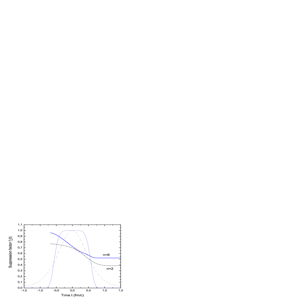
Figure 2: Time dependence of the suppression factor $f_{s}(t)$ for two types of field pulse, given by Eq. (32), with the same width: the pulse with $n=6$ (solid line) and the pulse with $n=2$ (dash-dotted line). Dotted and dashed lines show the corresponding field profiles.

Figure 3: Time dependence of particle densities normalized on its final value $n_{r}=n(t\gg\tau)$ for pulse (33) with the width $\tau_{0}=1$ fm/$c$.

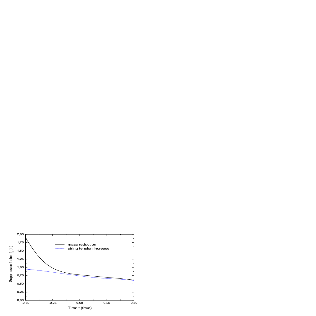
Figure 4: Comparison of two mechanisms of $f_{s}$ enhancement: the quark mass reduction (solid line) and the string tension increase (dotted line).

References

- (1) A. Casher, H. Neuberger, and A. Nussinov, Phys. Rev. D 20 (1979) 179; D 21 (1980) 1966.
- (2) B. Andersson et al., Phys. Rep. 97 (1983) 31; B. Andersson, G. Gustafson, and B. Nielsson-Almqvist, Nucl. Phys. B 281 (1987) 289.
- (3) A.B. Kaidalov, Surveys in High Energy Phys. 13 (1999) 265; A.B. Kaidalov and K.A. Ter-Martirosyan, Phys. Lett. B 117 (1982) 247.
- (4) N.S. Amelin and L.V. Bravina, Sov. J. Nucl. Phys. 51 (1990) 133; N.S. Amelin, K.K. Gudima, and V.D. Toneev, Sov. J. Nucl. Phys. 51 (1990) 1093.
- (5) K. Werner, Phys. Rep. 232 (1993) 87.
- (6) S.A. Bass et al., Prog. Part. Nucl. Phys. 41 (1998) 255; M. Bleicher et al., J. Phys. G 25 (1999) 1859.
- (7) J. Schwinger, Phys. Rev. 82 (1951) 664.
- (8) F. Antinori et al., WA97 Collaboration, Nucl. Phys. A 661 (1999) 130c.
- (9) J. Rafelski, Phys. Lett. B 62 (1991) 333.
- (10) T.S. Biro, H.B. Nielsen, and J. Knoll, Nucl. Phys. B 245 (1984) 449.
- (11) H. Sorge et al., Phys. Lett. B 289 (1992) 6.
- (12) N.S. Amelin, M.A. Braun, and C. Pajares, Phys. Lett. B 306 (1993) 312.
- (13) S. Soff et al., Phys. Lett. B 471 (1999) 89.
- (14) M. Bleicher et al., Phys. Rev. C 64 (2001) 011902.
- (15) R.-C. Wang and C.-Y. Wong, Phys. Rev. D 38 (1988) 348.
- (16) D.V. Vinnik, A.V. Prozorkevich, S.A. Smolyansky et al., Eur. Phys. J. C 22 (2001) 341; Few-Body Syst. 32 (2002) 23.
- (17) A.A. Grib, S.G. Mamaev, and V.M. Mostepanenko, Vacuum Quantum Effects in Strong External Fields (Friedmann Lab. Publ., St.-Petersburg, 1994).
- (18) G. Gatoff, A.K. Kerman, and T. Matsui, Phys. Rev. D 36 (1987) 114.
- (19) M. Asakawa and T. Matsui, Phys. Rev. D 43 (1991) 2871.
- (20) S.A. Smolyansky et al., hep-ph/9712377; S.M. Schmidt et al., Int. J. Mod. Phys. E 7 (1998) 709.
- (21) Y. Kluger, E. Mottola, and J.M. Eisenberg, Phys. Rev. D 58 (1998) 125015.
- (22) A. Gangulu, P.K. Kaw, and J. Parikh, Phys. Rev. D 48 (1993) R2983.
- (23) S.V. Popov, JETP Lett. 74 (2001) 133.
- (24) C.D. Roberts, S.M. Schmidt, and D.V. Vinnik, Phys. Rev. Lett. 87 (2001) 193902; 89 (2002) 153901.
- (25) S.M. Schmidt et al., Phys. Rev. D 59 (1999) 094005; J.C. Bloch et al., D 60 (1999) 1160011.
- (26) V.V. Skokov, S.A. Smolyansky, and V.D. Toneev, hep-ph/0210099.
- (27) U. Heinz, AIP Conf. Proc. 602 (2001) 281.
- (28) S. Ochs and U. Heinz, Ann. Phys. (NY) 266 (1998) 351.
- (29) A.V. Prozorkevich, S.A. Smolyansky, and S.V. Ilyin, hep-ph/0301169.
- (30) S.G. Mamaev and N.N. Trunov, Sov. J. Nucl. Phys. 30 (1979) 677.
- (31) Y. Kluger, J.M. Eisenberg, and B. Svetitsky, Int. J. Mod. Phys. E 2 (1993) 333.
- (32) N.B. Narozhnyi and A.I. Nikishov, Sov. J. Nucl. Phys. 11 (1970) 596; S.V. Popov, Sov. Phys. JETP 35 (1972) 659.
- (33) N.S. Amelin et al., Eur. Phys. J. C 22 (2001) 149.
- (34) F. Cooper, E. Mottola, and G.C. Nayak, Phys. Lett. B 555 (2003) 181.
- (35) J.D. Bjorken, Phys. Rev. D 27 (1983) 140.