Nuclear quantum transport for barrier problems

Abstract

A method is presented which allows one to introduce collective coordinates self-consistently, in distinction to the Caldeira-Leggett model. It is demonstrated how the partition function $\mathcal{Z}$ for the total nuclear system can be calculated to deduce information both on its level density as well as on the decay rate of unstable modes. For the evaluation of $\mathcal{Z}$ different approximations are discussed. A recently developed variational approach turns out superior to the conventional methods that include quantum effects on the level of local RPA. Dissipation is taken into account by applying energy smearing, simulating in this way the coupling to more complicated states. In principle, such a coupling must depend on temperature. Previous calculations along another microscopic approach show this fact to imply an intriguing variation of the transport coefficients of collective motion with $T$. The relevance of this feature is demonstrated for the thermal fission rate and for the formation probability of super-heavy elements.

1 Problems of the Caldeira-Leggett model
from nuclear physics point of view

The two most prominent examples of nuclear physics where processes are governed by (iso-scalar) motion across potential barriers are fusion and fission. In both cases dissipation may play an important role. For large excitation energies the process is dominated by thermal activation. With decreasing energies quantum effects become more and more important until at zero temperature mere quantum tunnelling is the only contribution at sub-barrier energies.

Dissipation in the collective degrees of freedom describes flow of energy to a large set of other, fastly relaxing degrees of freedom, commonly referred to as the ”heat bath” although in nuclear physics this notion requires greatest care. Sometime ago Caldeira-Leggett have suggested a model [1] which allows for an exact treatment of the bath degrees of freedom. This becomes possible at the expense of an oversimplification of both the bath itself as well as of its coupling to collective motion. Whereas this assumption does not seem to be very restrictive for applications in condensed matter physics, it violates essential requirements for nuclear collective motion [2]. Let us just mention the most serious deficiencies.

• In the nuclear case the collective degrees of freedom (CDOF) are not independent of the nucleonic ones, viz of the heat bath. Already the simplest condition on self-consistency implies that the shape of the mean field in which the nucleons move must vary in non-linear way with the CDOF.

• Even in the simple case of small amplitude collective motion, the frequencies are determined by RPA-like secular equations which differ essentially from those of the Caldeira-Leggett model [2].

• Related to this issue is the fact that the Caldeira-Leggett model is unable to make predictions for the evaluation of the transport coefficients for collective motion like potential energy, inertia and even for the strength of friction. All of them depend sensitively on both the collective coordinate as well as on temperature.

Without invoking the Caldeira-Leggett model so far quantum effects in nuclear dissipative dynamics were mainly treated applying real time propagation [2, 3], with the exception of [4]. Whereas the former approach is based on the deformed shell model in the novel approach one starts with a typical nuclear Hamiltonian of two body nature before CDOF are introduced, as shall be explained below.

2 Self-consistent dynamics for separable two body Hamiltonians

Suppose we are given the Hamiltonian with separable two body interaction of

$$\hat{\cal H}=\hat{H}+\frac{k}{2}\,\hat{F}\hat{F}\qquad\textrm{with}\qquad k<0\,.$$ (1)

It may be understood as one term in an expansion of the two body interaction into separable terms. For transport problems this ansatz has been used before applying the Bohm-Pines method of introducing collective coordinates, see [2] with further references given therein. These applications were based on a real time approach, implying that this method is limited to temperatures above a certain $T_{c}$. Here, we want to follow an imaginary time approach [6, 7, 4]. Different to the Bohm-Pines method the collective variable is introduced through a Hubbard-Stratonovich transformation in the functional integral for the partition function of (1) we arrive at the one body Hamiltonian

$$\hat{\cal H}_{\textrm{HS}}=\hat{H}+q(\tau)\hat{F}+\frac{1}{2|k|}q^{2}(\tau)$$ (2)

where the collective coordinate $q$ depends on the imaginary time $\tau=0\ldots\hbar/T$ and has been introduced self-consistently. After expanding the periodic collective “path” into a Fourier series $q(\tau)=q_{0}+\sum_{r\neq 0}q_{r}\,\exp(\textrm{i}\nu_{r}\tau)$ where $\nu_{r}=(2\pi/\hbar)Tr$ are the Matsubara frequencies the final form of the functional integral for the partition function reads

$${\cal Z}(T)=\frac{1}{\sqrt{2\pi|k|T}}\int dq_{0}\ \exp(-{\cal F}^{\textrm{SPA}}(T,q_{0})/T)\,C(T,q_{0})\,.$$ (3)

The $q_{0}$-integral represents the thermal fluctuations, while the quantum fluctuations with amplitudes $q_{r}$ that become important at low temperatures enter the remaining path integral for the “dynamical” corrections

$$C(T,q_{0})=\int{\cal D}^{\prime}q\ \exp\left(-\frac{A(T,q_{0})}{|k|T}\right)$$ (4)

where the “action” can be expanded like

$$A(T,q_{0})=\lambda_{rs}(T,q_{0})q_{r}q_{s}+\rho_{rst}(T,q_{0})q_{r}q_{s}q_{t}+\sigma_{rstu}(T,q_{0})q_{r}q_{s}q_{t}q_{u}+{\cal O}(q_{r}^{5})\,.$$ (5)

The exponential in (3) represents the partition function of the static part of the Hamiltonian (2) with ${\cal F}^{\textrm{SPA}}(q_{0})$ being the corresponding free energy. The simplest approximation to the dynamical corrections consists in neglecting them entirely: $C^{\textrm{SPA}}(T,q_{0})\equiv 1$ represents the classical limit and has been given the name Static Path Approximation (SPA) in the past [5].

The coefficient $\lambda_{rs}$ of the second order part of (5) can be expressed in terms of the response function $\chi(T,q_{0},\omega)$ that describes the changes of the average $\langle\hat{F}\rangle_{\omega}$ for small variations of the path $q(\omega)$ [4]:

$$\lambda_{rs}(T,q_{0})=\left(1+k\chi(T,q_{0},\omega)\right)\,\delta_{r,-s}=\frac{\prod_{\mu}(\nu_{r}^{2}+\omega_{\mu}^{2}(T,q_{0}))}{\prod_{k>l}(\nu_{r}^{2}+\omega_{kl}^{2}(q_{0}))}\,\delta_{r,-s}$$ (6)

Here, the $\omega_{\mu}$ are the local RPA frequencies and $\hbar\omega_{kl}=\epsilon_{k}-\epsilon_{l}$ are the energies of the intrinsic excitations associated to the static part of the Hamiltonian (2). In cases where $\lambda_{rs}$ is positive and sufficiently large a truncation of (5) after the second order will do and the remaining $q_{r\neq 0}$-integrals in ${\cal D}^{\prime}q$ can be evaluated exactly. One ends up with the result of the Perturbed Static Path Approximation (PSPA)

$$C^{\textrm{PSPA}}(T,q_{0})=\prod_{r>0}\lambda_{r}^{-1}(T,q_{0})$$ (7)

which takes into account quantum fluctuations on the level of local RPA [6, 7, 4]. As $\lambda_{rs}$ depends on temperature the condition $\lambda_{1}>0$ for the breakdown of this approximation due to diverging integrals can be transformed into the requirement $T>T_{0}$, where for the “crossover temperature” (note the similarity to the case of dissipative tunneling [8]) $T_{0}<T_{c}$ holds true [4].

The coefficients $\rho_{rst}$ and $\sigma_{rstu}$ of (5) have been calculated in [9] where the breakdown of the approximation has been shifted to $T_{0}/2$ by treating the $q_{1}$- and $q_{2}$-integrals in ${\cal D}^{\prime}q$ to fourth order analytically. Meanwhile an approximation has been developed [10] that takes over basic ideas of a variational principle suggested for one-dimensional systems in [11] and [12]. Choosing a suitable $A_{\Omega}^{q_{0}}$ the correction factor (4) can be rewritten as the average defined with respect to the weight $\exp(-A_{\Omega}^{q_{0}}/|k|T)$

$$C(T,q_{0})=\left\langle\exp\left(-\frac{A(T,q_{0})-A_{\Omega}^{q_{0}}}{|k|T}\right)\right\rangle\,.$$ (8)

In order to determine the best approximation to the equilibrium quantity ${\cal Z}(T)$ the convexity of the exponential $\langle\textrm{e}^{-x}\rangle\geq\textrm{e}^{-\langle x\rangle}$ can be used such that the following inequality can be exploited:

$$C(T,q_{0})\geq C^{\textrm{var}}(T,q_{0})=\exp\left(-\frac{\langle A(T,q_{0})-A_{\Omega}^{q_{0}}\rangle}{|k|T}\right)$$ (9)

For $A_{\Omega}^{q_{0}}$ the PSPA form is chosen but with the RPA frequencies $\omega_{\mu}(T,q_{0})$ replaced by a number of adjustable parameters $\Omega_{\mu}(T,q_{0})$. Maximizing the right hand side of (9) with respect to $\Omega_{\mu}(T,q_{0})$ gives an optimal approximation to the partition function (3).

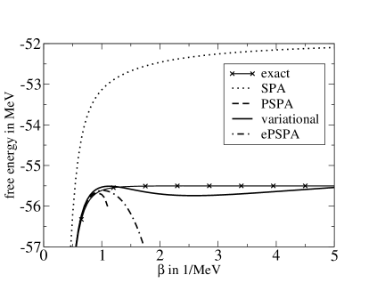
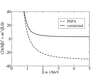
Figure 1: Left: Free energy of the LMG in various approximations. The variational principle gives very good results up to $\beta=1/T=5\,\textrm{MeV}^{-1}$ whereas the PSPA brakes down at $\beta_{0}=1/T_{0}=1.13\,\textrm{MeV}^{-1}$. Right: $\beta$-dependence of the quantities $\nu_{1}^{2}+\omega_{\textrm{RPA}}^{2}(q_{0}=0)$ and $\nu_{1}^{2}+\Omega_{\textrm{var}}^{2}(q_{0}=0)$.

In the left panel of fig. 1 we demonstrate at the example of the free energy of the exactly solvable Lipkin-Meshkov-Glick model (LMG) that the variational approach gives excellent results and is applicable even at very low temperatures. The classical SPA is good only at high temperatures. Inclusion of quantum effects on the RPA level via PSPA improves the approximation at high temperatures considerably but breaks down at $T_{0}$. The approximation of [9], called ePSPA, behaves well in the crossover region $T\approx T_{0}$. In order to illustrate the reason for the applicability of the variational principle at low temperatures we plot in the right panel of fig. 1 the $\beta$-dependence of the quantities $\nu_{1}^{2}+\omega_{\textrm{RPA}}^{2}(T,q_{0}=0)$ and $\nu_{1}^{2}+\Omega_{\textrm{var}}^{2}(T,q_{0}=0)$ that determine the sign of $\lambda_{1}$ and its variational analog via (6). The former quantity becomes negative at $\beta_{0}=1/T_{0}$ implying a breakdown of the PSPA, whereas the second one stays positive.

3 Introduction of dissipation and microscopic transport coefficients

So far dissipation has not been taken into account. The coefficient $\lambda_{r}(T,q_{0})$ of (6) contains the response function $\chi(\omega)=\chi^{\prime}(\omega)+\textrm{i}\chi^{\prime\prime}(\omega)$. In the independent particle model the dissipative part typically has the form (for $\omega>0$)

$$\chi^{\prime\prime}(\omega)=\sum_{k>l}f_{kl}\,\delta(\omega-\omega_{kl})$$ (10)

with strengths $f_{kl}$. We know that (at least at not too small excitations) the simple states of the independent particle model are coupled to more complicated ones via the residual interactions. The spectrum becomes more dense and the self-energy of the individual states acquires a finite width such that one ends up with a continuous function $\chi^{\prime\prime}(\omega)$. We do not go into these details [2] here but for simplicity mimic such effects by smearing out the spectrum by hand [4]. To such an averaged spectrum we fit the Lorentzian

$$\chi^{\prime\prime}(T,q_{0},\omega)=F^{2}(T,q_{0})\left(\frac{\Gamma(T,q_{0})/2}{(\omega-{\cal E}(T,q_{0}))^{2}+(\Gamma(T,q_{0})/2)^{2}}-({\cal E}\leftrightarrow-{\cal E})\right)$$ (11)

and extract the three parameters $F^{2}$, ${\cal E}$ and $\Gamma$. In this way the full response function may be interpreted locally as the one of a damped harmonic oscillator:

$$\chi(T,q_{0},\textrm{Im}z\neq 0)=\chi_{\textrm{osc}}=\frac{1}{M(T,q_{0})}\,\frac{1}{\omega_{\textrm{nucl}}^{2}(T,q_{0})-\textrm{i}\Gamma(T,q_{0})z-z^{2}}$$ (12)

The transport coefficients for the local inertia $M$, the local nucleonic frequency $\omega_{\textrm{nucl}}$ and the local damping $\Gamma$ can easily be related to the fit parameters [4] and depend on temperature $T$ and the collective coordinate $q_{0}$ simply because the original response function has those dependencies. One can easily convince oneself that the solution of the secular equation $1+k\chi(\omega)=0$ for the collective frequencies now has a finite imaginary part, indicating that collective motion is damped. The big advantage of the method suggested here is that all three transport coefficients $M$, $\omega_{\textrm{nucl}}$ and $\Gamma$ are taken from the same microscopic theory, instead of piecing together various macroscopic pictures.

In order to illustrate the drastic differences between our microscopic approach and the frequently used combination of wall friction, liquid drop stiffness and irrotational flow inertia we plot in fig. 2 the temperature dependence of some ratios of the transport coefficients for the barrier of ${}^{224}\textrm{Th}$.

Figure 2: Comparison of macroscopic (dashed) and microscopic (symbols) ratios of transport coefficients for the barrier of ${}^{224}\textrm{Th}$. The fully drawn line shows the simple analytical formulas proposed in [13]. Left: $\Gamma=\gamma/M=\hbar/\tau_{\textrm{kin}}$, often called $\beta$ in the literature. Right: The effective damping $\eta$. The dotted line indicates the change from under-damped ($\eta<1$) to over-damped ($\eta>1$) motion.

In the macroscopic picture the ratio $\Gamma=\gamma/M$ does not depend on temperature and is much larger than in the microscopic picture where it increases with temperature and vanishes at $T=0$. Within this macroscopic picture the effective damping strength $\eta=\gamma/(2\sqrt{|C|M})$ is strongly over-damped implying the applicability of the Smoluchowsky limit. For the microscopic transport coefficients, on the other hand, we observe a transition from under-damped motion ($\eta<1$) to over-damped motion ($\eta>1$); note that in the former case the inertia plays an important role. Even at $T=3\,\textrm{MeV}$ the Smoluchowsky limit is not fully reached.

4 Application I: Thermal fission

Applying a saddle point approximation to the $q_{0}$-integral in (3) we can calculate the rate of thermal fission from the imaginary part of the free energy from the formula [14, 15]

$$R(T)=-\frac{2}{\hbar}\,\frac{T_{0}}{T}\,\textrm{Im}\mathcal{F}(T)\qquad\textrm{for}\qquad T>T_{0}\,.$$ (13)

In situations where the potential is given by just one minimum located at $q=q_{a}$ and just one parabolic barrier at $q=q_{b}$ we obtain

$$R=\frac{\varpi(q_{b})}{2\pi}\ \sqrt{\frac{\mathcal{C}_{\mathcal{F}}(q_{a})}{|\mathcal{C}_{\mathcal{F}}(q_{b})|}}\ \left(\sqrt{1+\eta^{2}(q_{b})}-\eta(q_{b})\right)\ \textrm{e}^{-\mathcal{F}^{\textrm{SPA}}(q_{b})/T}\cdot\frac{C(q_{b})}{C(q_{a})}\,.$$ (14)

In order to simplify notation we have omitted the $T$-dependence everywhere. Besides the Arrhenius factor there appear non-trivial ones which are worth to be discussed in detail. The first two factors can be rewritten in the form $\varpi(q_{a})/2\pi\cdot\sqrt{M(q_{a})/M(q_{b})}$ where the attempt frequency at the minimum and the ratio of the inertias at the minimum and the barrier appear. The term in brackets is the famous Kramers factor [16] that takes into account the decrease of the decay rate due to damping. The last factor represents the increase of the rate due to quantum corrections. It has been calculated in [17] and [3] for the example of ${}^{224}\textrm{Th}$. While [17] use a Caldeira-Leggett type model, microscopic temperature- and coordinate dependent transport coefficients are used in [3]. Its contribution turns out to be significant at low temperatures (but with $T>T_{0}$).

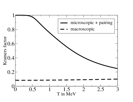
Figure 3: $T$-dependence of Kramers’ factor for macroscopic and microscopic transport coefficients.

In [13] the importance of microscopic transport coefficients for the description of thermal fission has been examined in more detail. It has been found that the experimentally observed phenomenon of “onset of dissipation” [18] cannot be explained by the macroscopic set of transport coefficients. In order to illustrate this statement we plot in fig. 3 the temperature dependence of Kramers’ factor. Using macroscopic transport coefficients no “onset of dissipation” can be seen at all, whereas for microscopic ones it appears around the $T\approx 0.5\,\textrm{MeV}$, exactly where pairing disappears.

5 Application II: Formation probabilities in fusion

Now we like to turn to a more recent application of microscopic $T$- and $q_{0}$-dependent transport coefficients to the probability of compound nucleus formation in production of super-heavy elements [19]. We do not study the initial phase of the reaction explicitly but make the assumption that due to dissipation the sum of the incident energy $E$ and the assumed barrier height $E_{b}=10\,\textrm{MeV}$ is distributed into a remaining kinetic energy and a thermal excitation according to

$$E_{0}^{\textrm{kin}}=R(E+E_{b})\qquad\textrm{and}\qquad E_{0}^{*}=(1-R)(E+E_{b})\,.$$ (15)

For the parameter $R$ we compare the effect of the two assumptions $R=0$ and $R=0.25$ on the final formation probability

$$\Pi_{\infty}=\frac{1}{2}\ \textrm{erfc}\left(-\frac{q_{\infty}}{\sqrt{2\Sigma_{qq}^{\infty}}}\right)$$ (16)

with

$$q_{\infty}=\sqrt{\frac{E_{0}^{\textrm{kin}}}{\hbar\varpi_{b}}}+\sqrt{\frac{E_{b}}{\hbar\varpi_{b}}}\,\frac{z^{-}}{\varpi_{b}}\qquad\textrm{where}\qquad\frac{z^{-}}{\varpi_{b}}=-\frac{\sqrt{1+\eta_{b}^{2}}+\eta_{b}}{2}$$ (17)

and

$$2\Sigma_{qq}^{\infty}=\frac{\Sigma_{pp}(t_{0})-\Sigma_{pp}^{eq,b}}{\hbar^{2}}+\left(\frac{z^{-}}{\varpi_{b}}\right)^{2}\left(\Sigma_{qq}(t_{0})-\Sigma_{qq}^{eq,b}\right)\,.$$ (18)

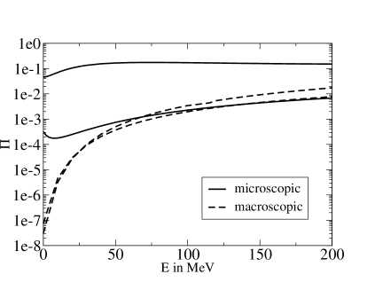
Figure 4: Formation probability as a function of incident energy. The initial conditions $\Sigma_{pp}(t_{0})=\Sigma_{pp}^{eq,b}$ of thermal equilibrium for the momentum distribution, $\Sigma_{qq}(t_{0})\Sigma_{pp}(t_{0})=3\hbar^{2}/4$ and $\Sigma_{qp}(t_{0})=0$ are used. Clearly these fluctuations are compatible with quantum mechanics.

In fig. 4 we compare the dependence of the formation probability on incident energy for microscopic transport coefficients with that of macroscopic ones. In both cases the upper curve corresponds to finite initial kinetic energy ($R=0.25$) whereas the lower one represents $R=0$. Most striking is the fact that for not too high incident energies the weak damping in the case of microscopic transport coefficients results in formation probabilities that are orders of magnitude larger than those of the macroscopic picture. In addition to that – as expected for the case of under-damped or slightly over-damped motion $\eta_{b}\approx 0.5\ldots 2$ – the microscopic formation probability is extremely sensitive to the initial kinetic energy. Such a dependence is very weak in the case of macroscopic transport coefficients. The reason is found in the fact that in this case motion is strongly over-damped $\eta_{b}\approx 5\ldots 6$.

6 Summary

We have developed a method for the description of dissipative collective motion in finite nuclei that does not suffer from the deficiencies of the Caldeira-Leggett model. This method enables one to calculate microscopically on the same footing transport coefficients for inertia, damping and stiffness, including their dependence on temperature and collective coordinate. Comparison with the macroscopic picture of the liquid drop model and wall friction shows significant differences, resulting in much weaker damping at low temperatures in general. These effects are shown to be important in thermal fission as well as in the formation of the compound nucleus in super-heavy element production.

References

- [1] A. O. Caldeira and A. J. Leggett, Ann. Phys. 149, 374 (1983); 153, 445(E) (1984).
- [2] H. Hofmann, Phys. Rep. 284 (4&5), 137 (1997).
- [3] H. Hofmann and F. A. Ivanyuk, Phys. Rev. Lett. 82, 4603 (1999).
- [4] C. Rummel and H. Hofmann, Phys. Rev. E 64, 066126 (2001).
- [5] B. Mühlschlegel, D. J. Scalapino and R. Denton, Phys. Rev. B 6, 1767 (1972).
- [6] G. Puddu, P. F. Bortignon, and R. A. Broglia, Ann. Phys. (San Diego) 206, 409 (1991).
- [7] H. Attias and Y. Alhassid, Nucl. Phys. A 625, 565 (1997).
- [8] H. Grabert and U. Weiss, Phys. Rev. Lett. 53, 1787 (1984); H. Grabert, P. Olschowski, and U. Weiss, Phys. Rev. B 36, 1931 (1987).
- [9] C. Rummel and J. Ankerhold, Eur. Phys. J. B 29, 105 (2002).
- [10] C. Rummel, H. Hofmann, to be published.
- [11] R. Giachetti and V. Tognetti, Phys. Rev. Lett. 55, 912 (1985); R. Giachetti and V. Tognetti, Phys. Rev. B 33, 7647 (1986).
- [12] R. P. Feynman and H. Kleinert, Phys. Rev. A 34, 5080 (1986).
- [13] H. Hofmann, F. A. Ivanyuk, C. Rummel, and S. Yamaji, Phys. Rev. C 64, 054316 (2001).
- [14] J. S. Langer, Ann. Phys. (N.Y.) 41, 108 (1967).
- [15] I. Affleck, Phys. Rev. Lett. 46, 388 (1981).
- [16] H. A. Kramers, Physica (Utrecht) 7, 284 (1940).
- [17] P. Fröbrich and G.-R. Tillack, Nucl. Phys. A 540, 353 (1992).
- [18] M. Thoennessen and G. F. Bertsch, Phys. Rev. Lett. 71, 4303 (1993).
- [19] C. Rummel and H. Hofmann, Nucl. Phys. A 727, 24 (2003).