Gamow Shell-Model Description of Weakly Bound and Unbound Nuclear States

Abstract

Recently, the shell model in the complex $k$-plane (the so-called Gamow Shell Model) has been formulated using a complex Berggren ensemble representing bound single-particle states, single-particle resonances, and non-resonant continuum states. In this framework, we shall discuss binding energies and energy spectra of neutron-rich helium and lithium isotopes. The single-particle basis used is that of the Hartree-Fock potential generated self-consistently by the finite-range residual interaction.

I Introduction

Low-energy nuclear physics is undergoing a revival with revolutionary progress in radioactive beam experimentation. New facilities have been built or are under construction, and new ambitious future projects, such as the Rare Isotope Accelerator in the U.S.A., will shape research in this field for decades to come. From a theoretical point of view, the major problem is to achieve a consistent picture of weakly bound and unbound nuclei, which requires an accurate description of the particle continuum properties when carrying out multi-configuration mixing. This is the domain of the continuum shell model [1] and, most recently, the Gamow Shell Model (GSM) [2, 3] (see also [4]). GSM is the multiconfigurational shell model with a single-particle (s.p.) basis given by the Berggren ensemble [5] which contains Gamow (or resonant) states and the complex non-resonant continuum. The resonant states are the generalized eigenstates of the time-independent Schrödinger equation which are regular at the origin and satisfy purely outgoing boundary conditions. The s.p. Berggren basis is generated by a finite-depth potential, and the many-body states are obtained in shell-model calculations as the linear combination of Slater determinants spanned by bound, resonant, and non-resonant s.p. basis states. Hence, both continuum effects and correlations between nucleons are taken into account simultaneously. An interested reader can find all details of the formalism in Refs. [2, 3] in which the GSM was applied to many-neutron configurations in neutron-rich helium and oxygen isotopes. In this contribution, we shall present the first application of the GSM formalism to the $p$-shell nuclei in the model space involving both neutron and proton s.p. Gamow states calculated from the self-consistent Hartree-Fock (HF) method (Gamow Hartree-Fock, GHF). Moreover, we briefly report on the first successful application of the density matrix renormalization group (DMRG) technique[6] in the context of realistic multiconfigurational shell model (SM).

II Description of the calculation

In our previous studies [2, 3], we have used the Surface Delta Interaction (SDI) and the s.p. basis has been generated by a Woods-Saxon (WS) potential which was adjusted to reproduce the s.p. energies in ⁵He. This potential (“⁵He” parameter set [3]) has the radius $R_{0}=2$ fm, the diffuseness $d=$0.65 fm, the strength of the central field $V_{0}=47$ MeV, and the spin-orbit strength $V_{so}=$7.5 MeV. The SDI interaction has several disadvantages in practical applications. Firstly, it has zero range, so one is forced to introduce an energy cutoff and, consequently, the residual interaction depends explicitly on the model space. Moreover, one is bound to use the same WS basis for all nuclei, as the SDI interaction cannot practically be used to generate the HF potential. Consequently, as the chosen WS basis is not an optimal s.p. basis (HF basis is), one cannot easily truncate the configuration space when the number of valence particles increases [3]. So, we have decided to introduce a new two-body residual interaction, the Surface Gaussian Interaction (SGI):

$$V_{J,T}(\vec{r_{1}},\vec{r_{2}})=V_{0}(J,T)\cdot\exp\left[-\left(\frac{\vec{r_{1}}-\vec{r_{2}}}{\mu}\right)^{2}\right]\cdot\delta{\left(|\vec{r_{1}}|+|\vec{r_{2}}|-2\cdot R_{0}\right)},$$ (1)

which is used together with the WS potential with the “⁵He” parameter set.

The SGI interaction is a compromise between the SDI and the Gaussian interaction. The parameter $R_{0}$ in Eq. (1) is the radius of the WS potential, and $V_{0}(J,T)$ is the coupling constant which explicitly depends on the total angular momentum $J$ and and the total isospin $T$ of the pair of nucleons. A principal advantage of the SGI is that it is finite-range, so no energy cutoff is needed. Moreover, the surface delta term in (1) simplifies the calculation of two-body matrix elements, because the radial integrals become one-dimensional and they extend from $r$=0 to $r$=2$R_{0}$. (In the Gaussian case, such as the Gogny force, they are two-dimensional and have to be extended to infinity.) Consequently, an adjustment of the Hamiltonian parameters becomes feasible. Finally, the resulting spherical HF potential is continuous and can be calculated very accurately. This allows one to use the optimal spherical HF potential for the generation of the Berggren basis for each nucleus studied; hence a more efficient truncation in the space of configurations with a different number of particles in the non-resonant continuum. In the present study, it turned out to be sufficient to consider at most two particles in the GHF continuum. This restriction on the number of particles in the non-resonant continuum allowed us to extend the studies up to unbound ¹⁰He and the halo nucleus ¹¹Li.

A Choice of the valence space

In our He and Li calculations, the valence space for protons and neutrons consists of $0p_{3/2}$ and $0p_{1/2}$ spherical GHF resonant states, calculated for each nucleus, and the $\{ip_{3/2}\}$ and $\{ip_{1/2}\}$ $(i=1,\cdots,M)$ complex continua generated by the same potential. These continua extend from $Re[k]$=0 to $Re[k]$=8 fm^-1 and they are discretized with 14 points (i.e., $M=14$). Altogether, we have 15 $p_{3/2}$ and 15 $p_{1/2}$ GHF states (shells) in the GSM calculation. The imaginary parts of $k$-values of the discretized continua are chosen to minimize the error made in calculating the imaginary parts of energies of the many-body states. Other continua, such as $s_{1/2}$, $d_{5/2}$, $\cdots$ are neglected, as they can be chosen to be real and would only induce a renormalization of the two-body interaction. We have checked [2, 3] that their influence on the binding energy of light helium isotopes is negligible. On the other hand, the $1s_{1/2}$ anti-bound neutron s.p. state is important in the heaviest Li isotopes (¹⁰Li, ¹¹Li) and plays a significant role in explaining the halo ground-state (g.s.) configuration of ¹¹Li [7, 8]. At present, however, solving a GSM problem for ¹¹Li in $[0p_{3/2},\{ip_{3/2}\};0p_{1/2},\{ip_{1/2}\};1s_{1/2},\{is_{1/2}\};(i=1,\cdots,M)]$ GHF space is not possible within a reasonable computing time. This task will be, however, possible in the near future by using a new generation GSM code which employs the DMRG methods to include the non-resonant continuum configurations contribution in the many-body wave function [9, 10].

Having defined a discretized GHF basis, one constructs the Slater determinants from all s.p. basis states (bound, resonant, and non-resonant), keeping only those with at most two particles in the non-resonant continuum. Indeed, as the two-body Hamiltonian is diagonalized in its optimal GHF basis, the weight of configurations involving more than two particles in the continuum is usually quite small, and they are neglected in the following.

B The Helium chain

Within the chain of helium isotopes, which are described assuming an inert ⁴He core, there are only $T$=1 two-body matrix elements. Consequently, only ($J$=0, $T$=1) and ($J$=2, $T$=1) couplings come into play. We have adjusted $V_{0}(J=0,T=1)$ to reproduce the experimental g.s. energy of ⁶He relative to the g.s. of ⁴He, whereas $V_{0}(J=2,T=1)$ has been fitted to all g.s. energies from ⁷He to ¹⁰He. Indeed, these latter states are mainly sensitive to $V_{0}(J=2,T=1)$ whereas, for obvious geometrical reasons, the $J=2,T=1$ coupling is absent in the g.s. of ⁶He. The adopted values are: $V_{0}(J=0,T=1)$ = –403 MeV fm³ and $V_{0}(J=2,T=1)$ = –315 MeV fm³.

The calculated spectrum of He isotopes is shown in Fig. 1. The experimental g.s. binding energies relative to the ⁴He core are reproduced fairly well. For instance, the g.s. of ⁶He and ⁸He are bound whereas ⁵He and ⁷He are unbound. Moreover, the so-called ‘helium anomaly’ (see, e.g., Ref. [15]), [i.e., the higher one- and two-neutron emission thresholds in ⁸He than in ⁶He], is well reproduced. The qualitative features seen in the experimental spectra are also satisfactorily reproduced by the GSM with the SGI Hamiltonian. The width of certain resonance states is too large mainly because these states are calculated at too high an excitation energy above the one- and two-nucleon emission threshold.

Looking at the configuration mixing in the g.s. of helium isotopes (see Tables I-V), one can see that the coupling to the non-resonant continuum is most important in ⁶He and ⁷He. This finding is consistent with the Borromean nature of ⁶He, which is bound only because of correlation effects (pairing scattering to the continuum). The g.s. of ⁷He is not a simple s.p. resonance, and this is reflected in GSM wave functions by large amplitudes of configurations involving particle(s) in the non-resonant continuum. This in turn implies that the g.s. width of ⁷He is a result of the complicated mixture of different configurations with three valence neutrons in various resonant and non-resonant shells.

The coupling to the continuum is somewhat less important in the heavier isotopes (⁸He, ⁹He, and ¹⁰He). This is partially related to the fact that these nuclei have a closed $0p_{3/2}$ shell; hence for the bound g.s. of ⁸He, the calculated spherical HF potential is the exact HF potential (no deformation effects are present). Consequently, the contributions of the 1p-1h excitations to the g.s. wave function vanish. For unbound states, there are small 1p-1h components due to the neglect of the imaginary part in the approximate HF potential used in the actual calculation. Secondly, in the heavier He isotopes, the GHF $0p_{3/2}$ shell is calculated to be bound, which further diminishes the importance of the coupling to the non-resonant continuum. Nevertheless, this coupling is by no means negligible, as the configurations involving states of the non-resonant continuum still represent about 10% of the wave function and play a significant role in generating binding for all these nuclei.

Comparing the SGI results with those of Ref. [3], one can see that the main conclusions for ⁶He and ⁷He still hold. This is because the HF potential for these nuclei is close to the WS potential which was previously used. However, once the $0p_{3/2}$ shell gets closed, the HF field becomes very different from the WS potential. As a consequence, the large configuration mixing obtained in Ref. [3] in the WS basis for ⁸He is significantly reduced when the GHF basis is used. In other words, a large part of the configuration mixing in the WS basis is not due to the presence of genuine two-particle correlations involving continuum states, but due to the 1p-1h couplings now incorporated in the GHF basis.

In order to assess the importance of two-particle correlations involving continuum states, we have calculated the g.s. of ⁶He, ⁷He, and ⁸He, but in the model space of 1p-1h excitations only. In such truncated calculations, the real part of the energy reads: 0.75 MeV for ⁵He, 0.58 MeV for ⁶He, 1.27 MeV for ⁷He, and –1.40 MeV for ⁸He. Based on these numbers, one is tempted to conclude that the anomalous increase of one- and two-neutron separation energies in ⁸He, as compared to ⁶He, is a genuine mean-field effect caused by the $J=2,T=1$ coupling. The coupling to the non-resonant continuum further enhances the helium anomaly.

The drip-line nucleus ⁸He is two-neutron bound already in the HF approximation, so the coupling to the non-resonant continuum provides only additional binding. On the other hand, ⁶He is unbound in GHF, so the continuum coupling is solely responsible for binding. Therefore, one may conclude that the Borromean features in the ^4-8He chain are caused mainly by the continuum couplings, whereas the helium anomaly is mainly due to the change from a ($J=0,T=1$)-dominated mean field to a mean field dominated by the ($J=2,T=1$) coupling.

C The Lithium chain

As a first example of GSM calculations in the space of proton and neutron states, we have chosen to investigate the Li chain. The continuum effects are very important in these nuclei, both in their ground states and in excited states. The nucleus ¹¹Li is also a well-known example of a two-neutron halo. In our $p$-space(s) calculation, we consider the one-body Coulomb potential of the ⁴He core, which is given by a uniformly charged sphere having the radius of the WS potential. It turns out that the inclusion of the one-body Coulomb potential modifies the GHF basis in lithium isotopes as compared to the helium isotopes, an effect which is usually neglected in the standard SM calculations.

Recent studies of the binding energy systematics in the $sd$-shell nuclei using the Shell Model Embedded in the Continuum (SMEC) have reported a significant reduction of the neutron-proton $T$=0 interaction with respect to the neutron-neutron $T$=1 interaction [16, 17] in the nuclei close to the neutron drip line. In SMEC [18], this reduction is associated with a decrease in the one-neutron emission threshold when approaching the neutron drip line, i.e., it is a genuine continuum coupling effect. The detailed studies in fluorine isotopes have shown that the reduction of the $T$=0 neutron-proton interaction cannot be corrected by any adjustment of the monopole components of the effective Hamiltonian. To account for this effect in the standard SM, one would need to introduce a $N$-dependence of the $T$=0 monopole terms. Interestingly, it has recently been suggested [19] that a linear reduction of $T$=0 two-body monopole terms is expected if one incorporates three-body interactions into the two-body framework of a standard SM.

Our GSM studies of lithium isotopes indicate that the reduction of $T$=0 neutron-proton interaction with increasing neutron number is essential. For example, if one uses the $V_{0}(J,T=0)$ strength adjusted to ⁶Li to calculate ⁷Li, the g.s. of ⁷Li becomes overbound by 13 MeV, and the situation becomes even worse for heavier Li isotopes. To reduce this disastrous tendency, in the first approximation we have used a linear dependence of $T$=0 couplings on the number of valence neutrons $n$:

$$V_{0}(J=1,T=0)=\alpha_{10}\left[1-\beta_{10}(n-1)\right],$$ (2)

(3)

$$V_{0}(J=3,T=0)=\alpha_{30}\left[1-\beta_{30}(n-1)\right],$$ (4)

with $\alpha_{10}=-600$ MeV fm³, $\beta_{10}=-50$ MeV fm³, $\alpha_{30}=-625$ MeV fm³, and $\beta_{30}=-100$ MeV fm³. This linear dependence is probably oversimplified, as shown in Refs. [16, 17] where the proton-neutron $T$=0 interaction first decreases fast with increasing neutron number and then saturates for weakly bound systems near the neutron drip line. For the $T$=1 interaction, we have taken the parameters $V_{0}(J=0,T=1)$ and $V_{0}(J=2,T=1)$ determined for the He chain (see Fig. 1 and the preceding discussion).

The results of our GSM calculations for the neutron-rich Li isotopes are shown in Fig. 2. One obtains a reasonable description of the g.s. energies of lithium isotopes relative to the g.s. energy of ⁴He, even though the agreement with the data is somewhat worse than in the He chain. Clearly, the particle-number dependence of the $T$=0 matrix elements has to be further investigated. The absence of an antibound $s_{1/2}$ state in the Berggren basis is most likely responsible for large deviations with the data seen in ¹⁰Li and ¹¹Li.

III Future perspectives: the Density Matrix Renormalization Group techniques for solving the Gamow Shell Model

As outlined above, in the GSM one uses a Berggren basis which consists of discrete states (bound and resonant states, $l=0$ anti-bound state for neutrons) and the discretized non-resonant continuum. Consequently, the dimension of the (non-hermitian) Hamiltonian matrix in GSM grows extremely fast with increasing the size of the Hilbert space. This ‘explosive’ growth of the dimension is much more severe than in the standard SM for which the dimensionality problem concerns only the ‘pole’ space of GSM. The future perspectives of GSM applications are ultimately related to the progress in developing new methods of truncating huge SM spaces. One promising approach is the DMRG method. In nuclear structure, this method has been successfully applied in schematic Hamiltonians [21], but no fully convincing results have so far been reported in the context of the realistic SM.

Let us begin by summarizing the basic elements of DMRG [6] (see also Ref. [21] for a pedagogical discussion relevant to nuclear physics applications). The main idea is to consider ‘step by step’ different s.p. shells in the configuration space and retain only the $N_{opt}$ “best states” dictated by the one-body density matrix. The convergence of the DMRG method is then studied with respect to $N_{opt}$.

The configuration space is divided into two subspaces denoted by ${\cal H}$ and ${\cal P}$. Generally speaking, ${\cal H}$ contains the lowest s.p. shells. In the first step, one calculates and stores all the possible matrix elements of suboperators of the Hamiltonian in the ${\cal H}$ space:

$$a^{\dagger},(a^{\dagger}\,\widetilde{a})^{j},(a^{\dagger}a^{\dagger})^{j},((a^{\dagger}a^{\dagger})^{j}\widetilde{a})^{J}),((a^{\dagger}a^{\dagger})^{j}(\widetilde{a}\widetilde{a})^{j})).$$

One also constructs in ${\cal H}$ all states $|h\rangle$ with $0,1,2,\cdots$ particles coupled to all possible $J$-values. Then, one considers the first s.p. shell in ${\cal P}$, calculates matrix elements of all suboperators in this shell, and constructs in ${\cal P}$ all states $|p\rangle$ with $0,1,2,\cdots$ particles coupled to all possible $J$-values. In the following, one adds ‘one by one’ additional s.p. shells in ${\cal P}$: one calculates all matrix elements of suboperators in the added shell and all states with $0,1,2,\cdots$ particles in the added shell and in the shell previously considered in ${\cal P}$. New states are successively added in ${\cal P}$ until the number of states $|p\rangle$ with $0,1,2,\cdots$ particles is larger than $N_{opt}$. Then one diagonalizes the Hamiltonian in the space $|hp\rangle^{J}$ made of vectors in ${\cal H}$ and ${\cal P}$. Obviously, the number of particles in such states is equal to the total number of valence particles in the system, and $J$ is equal to the angular momentum of the state of interest. From the eigenstates :

$$\Psi=\sum c_{hp}|hp\rangle^{J},$$ (5)

one calculates the one-body density matrix:

$$\rho_{pp^{\prime}}=\sum_{h}c_{hp}c_{hp^{\prime}}.$$ (6)

The density matrix is diagonalized and only $N_{opt}$ eigenstates having the largest eigenvalues are retained. (In the non-hermitian GSM problem, eigenvalues of the density matrix are complex and the eigenstates are selected according to the largest absolute value of the density eigenvalues.) One then recalculates all the matrix elements of suboperators for the optimized states; they are linear combinations of previously calculated matrix elements. Then, one adds the next shell in ${\cal P}$ and, again, only the $N_{opt}$ states selected according to the above prescription are kept. This procedure is continued until the last shell in ${\cal P}$ is reached, providing a ‘first guess’ for the many-body wave function.

At this stage, a “sweeping phase” begins in which the iterative process is reversed. First, one considers the last shell in ${\cal P}$. At this point, one constructs states with $0,1,2,\cdots$ particles and then the process continues, step by step, until the number of vectors becomes larger than $N_{opt}$. When the $i^{th}$ shell in ${\cal P}$ is reached, the Hamiltonian is diagonalized in the set of vectors $|h,p_{prev},p\rangle^{J}$, where $h$ is a state that belongs to ${\cal H}$, $p_{prev}$ is a previously optimized state ($i$–1 first shells in ${\cal P}$), and $p$ is a state that concerns all the shells between the $i^{th}$ one and the last one in ${\cal P}$. The density matrix is then diagonalized and the $N_{opt}$ $p$-states are kept. The procedure continues by adding the $(i-1)^{st}$ shell in ${\cal P}$, etc., until the first state is reached. Then the procedure is reversed: the first shell is added, then the second, the third, etc. The succession of sweeps is successful if the energy gradually converges after every sweep.

As a first application of DMRG, we calculated the g.s. $0_{1}^{+}$ and the excited $0_{2}^{+}$ state in ⁶He in the same configuration space as in Sec. II B. Initially, we applied the DMRG procedure without sweeping, i.e., in its ‘infinite algorithm’ version [6]. In this calculation, we considered 14 $p_{1/2}$ shells and 14 $p_{3/2}$ shells in the non-resonant continuum. The method succeeded in reproducing the “exact” g.s. energy of ⁶He when taking 16 shells in ${\cal H}$ (8 $p_{1/2}$ shells and 8 $p_{3/2}$ shells) and keeping 6 vectors in ${\cal P}$ at each iteration. One should mention that the states in ${\cal H}$ have not been optimized during the iterative procedure. This example demonstrates that the DMRG in the infinite-system variant can be generalized for genuinely non-hermitian problems. On the other hand, the resulting gain in reducing the dimensionality of the GSM is not particularly impressive.

The gain factor is radically improved when the finite-system algorithm (sweeping) is applied. In this case, for 20 $p_{1/2}$ shells and 20 $p_{3/2}$ shells in the non-resonant continuum, an excellent convergence has been reached for both states of ⁶He by taking $0p_{1/2}$ and $0p_{3/2}$ Gamow resonances in ${\cal H}$ and keeping in ${\cal P}$ only six vectors after adding each shell. In the considered example, the total dimension of the GSM Hamiltonian is 462 and the rank of the biggest matrix to be diagonalized in GSM+DMRG is 32. The gain factor is expected to be even more impressive for a larger number of valence particles.

IV Conclusions

The Gamow Shell Model, which has been introduced only very recently [2, 3], has proven to be a reliable tool for the microscopic description of weakly bound and unbound nuclear states. In He isotopes, GSM with either SDI or SGI interactions was able to describe fairly well the many-body properties, in particular the Borromean features in the chain ^4-8He. Using the finite-range SGI interaction made it possible to perform GHF calculations, thus designing the optimal Berggren basis for each nucleus. In this way, we were able to disentangle the correlations due to the continuum coupling from the particle-hole excitations essential for building the mean field. We have shown that the Borromean features of the helium isotopes are the results of the correlations involving the non-resonant continuum, whereas the helium anomaly is a mean field effect due to the transition from a ($J=0,T=1$)-dominated mean field in ⁶He to the ($J=2,T=1$) GHF field in ⁸He.

In Li isotopes, $T$=0 matrix elements of the two-body interaction could be studied for bound and resonant many-body states. It was found that the $T$=0 interaction contains a pronounced density (particle-number) dependence which originates from the coupling to the continuum and leads to an effective renormalization of the neutron-proton coupling. This effect cannot be absorbed by the modification of $T$=0 monopole terms in the standard SM framework. The effective renormalization of ($J=1,T=0$) and ($J=3,T=0$) couplings, which has been found in the present GSM studies, has to be further investigated, as it is also related to the question about the importance of 3-body correlations and density dependence.

The successful application of GSM to heavier nuclei is ultimately related to the progress in optimization of the GSM basis. The promising development, discussed in this paper, is the adaptation of the DMRG method [6] to the genuinely non-hermitian SM problem in the complex-$k$ plane. The first applications using the $j$-scheme GSM are very promising; they demonstrate that we may well be at the edge of solving the GSM in today’s inaccessible model spaces.

This work was supported in part by the U.S. Department of Energy under Contract Nos.  DE-FG02-96ER40963 (University of Tennessee) and DE-AC05-00OR22725 with UT-Battelle, LLC (Oak Ridge National Laboratory), DE-FG05-87ER40361 (Joint Institute for Heavy Ion Research), and by the Polish Committee for Scientific Research (KBN).

TABLE I.: Squared amplitudes of configurations in the ground state of ⁶He. The sum of squared amplitudes of Slater determinants with $n$ particles in the continuum is denoted by $L_{+}^{(n)}$.

Configuration	$c^{2}$
$0p^{2}_{3/2}$	0.656–i0.566
$0p^{2}_{1/2}$	6.06$\cdot 10^{-3}$–i0.0516
$L_{+}^{(1)}$	0.363+i0.509
$L_{+}^{(2)}$	–0.0245+i0.108

TABLE II.: Similar as in Table I except for the $3/2^{-}_{1}$ g.s. of ⁷He.

Configuration	$c^{2}$
$0p^{3}_{3/2}$	0.331–i0.0973
$0p^{1}_{3/2}$ $0p^{2}_{1/2}$	0.0111–i0.0406
$0p^{2}_{3/2}$ $0p^{1}_{1/2}$	5.380$\cdot 10^{-4}$–i6.950$\cdot 10^{-4}$
$L_{+}^{(1)}$	0.507+i0.0714
$L_{+}^{(2)}$	0.150+i0.0672

TABLE III.: Similar as in Table I except for the g.s. of ⁸He.

Configuration	$c^{2}$
$0p^{4}_{3/2}$	0.889–i7.826$\cdot 10^{-3}$
$0p^{2}_{3/2}$ $0p^{2}_{1/2}$	0.0316–i0.0529
$L_{+}^{(1)}$	0.0613+i0.0226
$L_{+}^{(2)}$	0.0184+i0.0225

TABLE IV.: Similar as in Table I except for the $1/2^{-}_{1}$ g.s. of ⁹He.

Configuration	$c^{2}$
$0p^{4}_{3/2}$ $0p^{1}_{1/2}$	0.937–i0.0209
$L_{+}^{(1)}$	0.0473–i1.779$\cdot 10^{-3}$
$L_{+}^{(2)}$	0.0157+i0.0227

TABLE V.: Similar as in Table I except for the g.s. of ¹⁰He.

Configuration	$c^{2}$
$0p^{4}_{3/2}$ $0p^{1}_{1/2}$	0.965–i0.0206
$L_{+}^{(1)}$	-5.640$\cdot 10^{-3}$+i8.392$\cdot 10^{-3}$
$L_{+}^{(2)}$	0.0409+i0.0122

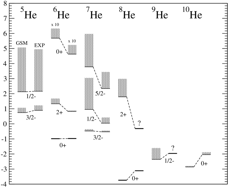
FIG. 1.: GSM spectra of helium isotopes obtained with the SGI Hamiltonian. Experimental data are taken from Refs. [11, 12, 13, 14].

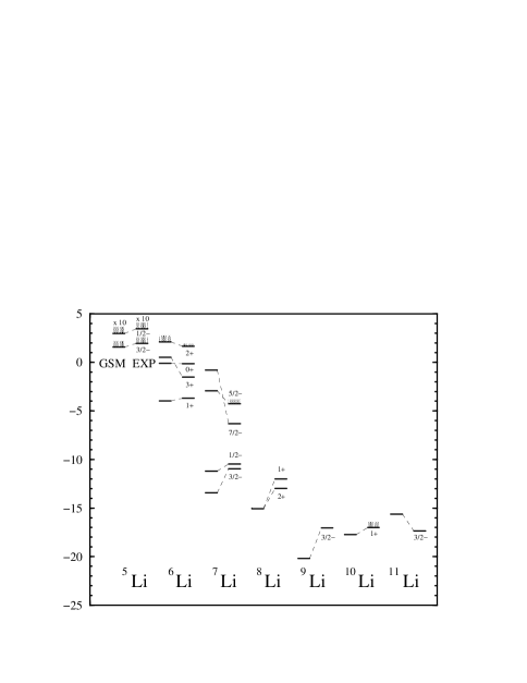
FIG. 2.: GSM spectra of lithium isotopes obtained with the SGI Hamiltonian. Experimental data are taken from Refs. [11, 12, 20].

REFERENCES

- [1] J. Okołowicz, M. Płoszajczak, and I. Rotter, Phys. Rep. 374 (2003) 271.
- [2] N. Michel, W. Nazarewicz, M. Płoszajczak, and K. Bennaceur, Phys. Rev. Lett. 89 (2002) 042502.
- [3] N. Michel, W. Nazarewicz, M. Płoszajczak, and J. Okołowicz, Phys. Rev. C67 (2003) 054311.
- [4] R. Id. Betan, R.J. Liotta, N. Sandulescu, and T. Vertse, Phys. Rev. Lett. 89 (2002) 042501.
- [5] T. Berggren, Nucl. Phys. A109 (1968) 265.
- [6] S.R. White, Phys. Rev. B48 (1993) 10345; Phys. Rev. B48 (1993) 10345.
- [7] I.J. Thompson and M.V. Zhukov, Phys. Rev. C49 (1994) 1904.
- [8] R. Id Betan, R.J. Liotta, N. Sandulescu, and T. Vertse, nucl-th/0307060.
- [9] J. Rotureau, PhD-thesis, University of Caen (2004).
- [10] J. Rotureau, N. Michel, W. Nazarewicz, M. Płoszajczak, and J. Dukelsky, in preparation.
- [11] Evaluated Nuclear Structure Data File, http://www.nndc.bnl.gov/nndc/ensdf.
- [12] Nuclear structure and decay data, http://nucleardata.nuclear.lu.se/database/masses/.
- [13] M. Meister et al., Phys. Rev. Lett. 88 (2002) 102501.
- [14] H.G. Bohlen et al., Nucl. Phys. A583 (1995) 775c .
- [15] A.A. Oglobin and Y.E. Penionzhkevich, in Treatise on Heavy-Ion Science, Nuclei Far From Stability, Vol. 8, Plenum, New York, 1989, edited by D.A. Bromley, p. 261.
- [16] Y. Luo, J. Okołowicz, M. Płoszajczak, and N. Michel, nucl-th/0201073.
- [17] N. Michel, W. Nazarewicz, J. Okołowicz, M. Płoszajczak, and J. Rotureau, in Proc. XXVIII Mazurian Lakes Conference on Physics, September 2003, Krzyże, Poland, Acta Phys. Pol. (2004).
- [18] K. Bennaceur, F. Nowacki, J. Okołowicz, and M. Płoszajczak, Nucl. Phys. A651 (1999) 289 and A671 (2000) 203.
- [19] A. Zuker, Phys. Rev. Lett. 90 (2003) 042502.
- [20] H.G. Bohlen et al., Nucl. Phys. A616 (1997) 254c.
- [21] J. Dukelsky, S. Pittel, S.S. Dimitrova, and M.V. Stoitsov, Phys. Rev. C65 (2002) 054319.